Solvable spectral problems from 2d CFT and ${\cal N}=2$ gauge theories

Abstract

The so-called 2d/4d correspondences connect two-dimensional conformal field theory (2d CFT), ${\cal N}=2$ supersymmetric gauge theories and quantum integrable systems. The latter in the simplest case of the SU(2) gauge group are nothing but the quantum-mechanical systems. In the present article we summarize our recent results and list open problems concerning an application of the aforementioned dualities in the studies of spectral problems for some Schrödinger operators with Mathieu–type periodic, periodic PT–symmetric and (Heun’s) elliptic potentials.

1 Introduction

They have long been known connections between ${\cal N}=2$ supersymmetric Yang–Mills theories and integrable models. Let us consider perhaps the simplest example of such a relationship, i.e., a link between the SU(2) pure gauge Seiberg–Witten theory and the one-dimensional sine-Gordon model (cf. [1]). Concretely, the statement here is that the Bohr–Sommerfeld periods

$$\Pi(\Gamma)\equiv\oint\limits_{\Gamma}P_{0}(\varphi)\,{\rm d}\varphi=\oint\limits_{\Gamma}\sqrt{2(u-\hat{\Lambda}^{2}\cos\varphi)}\,{\rm d}\varphi$$

for the classical sine-Gordon model defined by ${\cal L}_{\rm sG}=\frac{1}{2}\dot{\varphi}^{2}-\hat{\Lambda}^{2}\cos\varphi$, and for two complementary contours $\Gamma=A,B$ encircling two turning points $\pm\arccos(u/\hat{\Lambda}^{2})$ define the Seiberg–Witten system [2]: $a=\Pi(A)$, $\partial{\cal F}(a)/\partial a=\Pi(B)$. Here, $a$ is a modulus and ${\cal F}(a)$ denotes the Seiberg–Witten prepotential determining the low energy effective dynamics of the four-dimensional ${\cal N}=2$ supersymmetric SU(2) pure gauge theory.

As has been observed in [3] (see also [4, 5]) the above statement has its ‘quantum analogue’ or ‘quantum extension’ which can be formulated as follows. Namely, the monodromies (exact BS periods)

$$\widetilde{\Pi}(\Gamma)\equiv\oint\limits_{\Gamma}P(\varphi,\hbar)\,{\rm d}\varphi,\;\;\;\;P(\varphi,\hbar)=P_{0}(\varphi)+P_{1}(\varphi)\hbar+P_{2}(\varphi)\hbar^{2}+\ldots$$

of the exact WKB solution

$$\psi(\varphi)=\exp\left\{\frac{i}{\hbar}\int\limits^{\varphi}P(\rho,\hbar)\,{\rm d}\rho\right\}\;\;\;\rm{to\;the\;eq.}\;\;\;\boxed{\left[-\frac{\hbar^{2}}{2}\frac{\partial^{2}}{\partial\varphi^{2}}+\hat{\Lambda}^{2}\cos\varphi\right]\psi(\varphi)\;=\;\mathrm{E}\,\psi(\varphi)}$$ (1)

define the Nekrasov–Shatashvili system [6]: $a=\widetilde{\Pi}(A)$, $\partial{\cal W}(\hat{\Lambda},a,\hbar)/\partial a=\widetilde{\Pi}(B)$. Here, ${\cal W}(\hat{\Lambda},a,\hbar)={\cal W}_{\rm pert}(\hat{\Lambda},a,\hbar)+{\cal W}_{\rm inst}(\hat{\Lambda},a,\hbar)$ is the effective twisted superpotential of two-dimensional SU(2) pure gauge ($\Omega$-deformed) SYM theory defined in [6] as the following Nekrasov–Shatashvili (NS) limit

$${\cal W}(\hat{\Lambda},a,\hbar)\;\equiv\;\lim_{\epsilon_{2}\to 0}\epsilon_{2}\log{\cal Z}(\hat{\Lambda},a,\epsilon_{1}\!\!=\hbar,\epsilon_{2})$$

of the Nekrasov partition function ${\cal Z}(\hat{\Lambda},a,\epsilon_{1},\epsilon_{2})={\cal Z}_{\rm pert}(\hat{\Lambda},a,\epsilon_{1},\epsilon_{2}){\cal Z}_{\rm inst}(\hat{\Lambda},a,\epsilon_{1},\epsilon_{2})$ [8, 9].

Interestingly, on the other hand the Mathieu equation written in (1) is nothing but the Schrödinger equation for the sine-Gordon model. One can show that the energy eigenvalue is determined by the SU(2) pure gauge twisted superpotential ($\hbar=\epsilon_{1}$) [3, 10]:

$$2\textrm{E}_{\rm sG}=2\textrm{E}(a) = a^{2}+\hat{\Lambda}^{4}\left(\frac{1}{2\,a^{2}}+\frac{\epsilon_{1}^{2}}{8\,a^{4}}+\frac{\epsilon_{1}^{4}}{32\,a^{6}}+\frac{\epsilon_{1}^{6}}{128\,a^{8}}\right)$$

$$+ \hat{\Lambda}^{8}\left(\frac{5}{32\,a^{6}}+\frac{21\,\epsilon_{1}^{2}}{64\,a^{8}}+\frac{219\,\epsilon_{1}^{4}}{512\,a^{10}}+\frac{121\,\epsilon_{1}^{6}}{256\,a^{12}}\right)$$

$$+ \hat{\Lambda}^{12}\left(\frac{9}{64\,a^{10}}+\frac{55\,\epsilon_{1}^{2}}{64\,a^{12}}+\frac{1495\,\epsilon_{1}^{4}}{512\,a^{14}}+\frac{4035\,\epsilon_{1}^{6}}{512\,a^{16}}\right)+\mathcal{O}(\hat{\Lambda}^{16})$$

$$= \frac{1}{2}\epsilon_{1}\hat{\Lambda}\partial_{\hat{\Lambda}}\mathcal{W}^{N_{f}=0,{\rm SU(2)}}.$$

The fact that the eigenvalue of the Mathieu operator is given by $\hat{\Lambda}\partial_{\hat{\Lambda}}\mathcal{W}^{N_{f}=0,{\rm SU(2)}}$ is an example of the Bethe/gauge correspondence discovered by Nekrasov and Shatashvili [6]. The Bethe/gauge correspondence maps supersymmetric vacua of the ${\cal N}=2$ theories to Bethe states of some quantum integrable systems (QIS). A result of that duality is that the twisted superpotentials for SU(N) theories are identified with the Yang–Yang (YY) functions which describe spectra of the corresponding N–particle quantum integrable systems.

As has been already mentioned the twisted superpotentials are defined as the NS limit of the Nekrasov partition functions. The latter play also a key role in another relation — the celebrated AGT correspondence [11]. Indeed, let $C_{g,n}$ denotes the Riemann surface with genus $g$ and $n$ punctures. A significant part of the AGT conjecture is an exact correspondence between the Virasoro conformal blocks on $C_{g,n}$ and the instanton sectors of the Nekrasov partition functions of certain SU(2) quiver gauge theories belonging to some class $S_{g,n}$. It turns out that the NS limit of the Nekrasov functions corresponds to the so-called classical limit of conformal blocks [12]. Hence, combining the classical/NS limit of the AGT duality and the Bethe/gauge correspondence one thus gets the triple correspondence which links the classical Virasoro blocks to the SU(2) twisted superpotentials and then to spectra of some Schrödinger operators (see Fig.1). Indeed, let us note that 2-particle QIS are nothing but the quantum–mechanical systems.

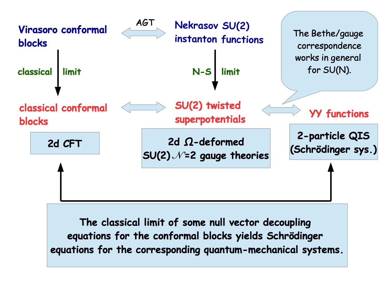
Figure 1: The triple correspondence in the case of the Virasoro classical conformal blocks links the latter to SU(2) instanton twisted superpotentials which describe the spectra of some quantum–mechanical systems. The Bethe/gauge correspondence on the r.h.s. connects the SU(N) ${\cal N}=2$ SYM theories with the N–particle quantum integrable systems. An extension of the above triple relation to the case ${\rm N}>2$ needs to consider on the l.h.s. the classical limit of the $W_{\rm N}$ symmetry conformal blocks according to the known extension [13] of the AGT conjecture.

Motivated by the aforementioned correspondences, we have studied in [10, 14, 15, 16] examples of a direct link between ‘classical’ 2d CFT (i.e., the classical, large central charge limit of the BPZ equations [17] obeyed by certain degenerate conformal blocks) and the corresponding quantum–mechanical models (= certain stationary Schrödinger equations), cf. Fig.1. In sections 2 and 3 of the present article we review main results of these investigations. In conclusions we explain our motivations and present some open problems for further studies.

In the rest of the introduction, in order to spell out our results, we remind a definition and some properties of quantum and classical conformal blocks. To begin with, let us recall that basic ingredients of any CFT model defined on Riemann surface $C_{g,n}$ are the correlation functions of the primary fields [17, 18]. Thanks to conformal symmetry any correlation function of the primary and descendants fields can be derived once the conformal blocks and structure constants are known. The conformal blocks are model independent CFT ‘special functions’ defined entirely within a representation theoretic framework.

Indeed, let ${\cal V}_{c,\Delta}^{n}$ denotes the vector space generated by all vectors of the form:

$$|\,\Delta^{n}_{I}\,\rangle=L_{-I}|\,{\Delta}\,\rangle\equiv L_{-k_{1}}\ldots L_{-k_{\ell(I)}}|\,{\Delta}\,\rangle,\;\;\;\;\;\;\;\;n=k_{1}+\ldots+k_{\ell(I)}=:|I|,$$ (2)

where $I=(k_{1}\geq\ldots\geq k_{\ell(I)}\geq 1)$ is a partition of $n$, $L_{n}$’s are the Virasoro generators obeying

$$[L_{n},L_{m}]=(n-m)L_{n+m}+\frac{c}{12}(n^{3}-n)\delta_{n+m,0},$$ (3)

and $|\,\Delta\,\rangle$ is the highest weight state with the following property:

$$L_{0}|\,\Delta\,\rangle=\Delta|\,\Delta\,\rangle,\;\;\;\;\;\;\;\;\;\;\;L_{n}|\,\Delta\,\rangle=0,\;\;\;\;\forall\;n>0.$$ (4)

The representation of the Virasoro algebra on the space:

$${\cal V}_{c,\Delta}=\bigoplus\limits_{n=0}^{\infty}{\cal V}_{c,\Delta}^{n},\;\;\;\;\;\;\;{\cal V}_{c,\Delta}^{0}=\mathbb{R}|\,\Delta\,\rangle$$

defined by the relations (3), (4) is called the Verma module with the central charge $c$ and the highest weight $\Delta$. It is clear that $\dim{\cal V}_{c,\Delta}^{(n)}={\sf p}(n)$, where ${\sf p}(n)$ is the number of partitions of $n$ (with the convention ${\sf p}(0)=1$). On ${\cal V}_{c,\Delta}^{(n)}$ exists symmetric bilinear form $\langle\,\cdot\,|\,\cdot\,\rangle$ uniquely defined by the relations $\langle\,\Delta\,|\,\Delta\,\rangle=1$ and $(L_{n})^{\dagger}\;=\;L_{-n}$.

Let $|\,0\,\rangle$ denotes the vacuum state, i.e., the highest weight state in the vacuum module with the highest weight $\Delta=0$. The conformal blocks on the Riemann sphere are defined as the matrix elements

$$\langle\,0\,|V_{\Delta_{n}}(z_{n})\ldots V_{\Delta_{1}}(z_{1})|\,0\,\rangle_{\rm sphere}$$

of compositions of the primary chiral vertex operators (CVO’s):

$$V_{\Delta_{j}}(z) \equiv V_{\alpha_{k},\alpha_{i}}^{\;\alpha_{j}}(z):{\cal V}_{\Delta_{i}}\longrightarrow{\cal V}_{\Delta_{k}},\;\;\;\;\;\;\;\;\Delta_{l}=\Delta_{\alpha_{l}}=\alpha_{l}(Q-\alpha_{l}),$$

$$\left[L_{n},V_{\Delta}(z)\right] = z^{n}\left(z\frac{\rm d}{{\rm d}z}+(n+1)\Delta\right)V_{\Delta}(z),\;\;\;\;\;\;\;\;n\in\mathbb{Z}.$$

acting between the Verma modules. The conformal blocks on the torus are traced cylinder matrix elements of 2d Euclidean ‘space-time’ translation operators and CVO’s insertions, i.e., ‘chiral partition functions’. The conformal blocks on the higher genus Riemann surfaces can be constructed by making use of the so-called sewing or gluing procedure.

By inserting projection operators $\mathbb{P}_{\tilde{\Delta}_{p}}$ on the intermediate conformal weights $\tilde{\Delta}_{p}$, $p=1,\ldots,3g-3+n$ into the internal channels of the conformal blocks one gets the latter in terms of the formal power series. In the simplest cases, namely, for the 4-point block on the sphere and the 1-point block on the torus the coefficients of the power series are implicitly defined via recursive relations. Up to now these coefficient are not been computed in closed form in the general case.

Taking into account a number of recent applications one of central issues concerning the conformal blocks is the existence of their classical limit. This is the limit in which all parameters of the conformal blocks tend to infinity in such a way that their ratios are fixed:

$$\Delta_{i},\;\tilde{\Delta}_{p},\;c\;\longrightarrow\;\infty,\;\;\;\;\;\;\;\;\;\;\;\;\frac{\Delta_{i}}{c}\;=\;\frac{\tilde{\Delta}_{p}}{c}\;=\;{\rm const.}\;\;\;,$$

$i=1,\ldots,n$, $p=1,\ldots,3g-3+n$. For the standard parametrization of the central charge $c=1+6Q^{2}$, where $Q=b+\frac{1}{b}$ and for ‘heavy’ weights $(\tilde{\Delta}_{p},\Delta_{i})=\frac{1}{b^{2}}(\tilde{\delta}_{p},\delta_{i})$ with $\tilde{\delta}_{p},\delta_{i}={\cal O}(b^{0})$ the classical limit corresponds to $b\to 0$. There exist many convincing arguments, but there is no proof, that in the classical limit the conformal blocks exponentiate to the functions $f_{\tilde{\delta}_{p}}(\delta_{i},Z)$ known as the classical conformal blocks [12, 19], e.g.:

$$\langle\,0\,|V_{\Delta_{n}}(z_{n})\mathbb{P}_{\tilde{\Delta}_{n-1}}\ldots\mathbb{P}_{\tilde{\Delta}_{2}}V_{\Delta_{1}}(z_{1})|\,0\,\rangle_{\rm sphere}\;\stackrel{{\scriptstyle b\to 0}}{{\sim}}\;{\rm e}^{\frac{1}{b^{2}}f_{\tilde{\delta}_{p}}(\delta_{i},Z)},\;\;\;\;\;\;\;\;\;Z:=(z_{n},\ldots,z_{1}).$$

The conformal blocks may also include the ‘light’ conformal weights ${\Delta}_{\sf light}$ which are defined by the property $\lim_{b\to 0}b^{2}{\Delta}_{\sf light}=0$. It is known, but not proven in general, that light insertions have no influence to the classical limit, i.e., do not contribute to the classical blocks:

$$\left\langle V_{\Delta_{\sf light}}(w)\prod_{i=1}^{n}V_{\Delta_{\sf heavy}}(z_{i})\right\rangle_{\!\!\rm sphere}\;\stackrel{{\scriptstyle b\to 0}}{{\sim}}\;\Psi(w)\;{\rm e}^{\frac{1}{b^{2}}f_{\tilde{\delta}_{p}}(\delta_{i},Z)}.$$ (5)

Due to the discovery of the AGT correspondence a considerable progress in the theory of conformal blocks has been recently achieved. In particular, Gaiotto analyzing an extension of the AGT conjecture to the class of the so-called ‘non-conformal’ ${\cal N}=2$, SU(2) super Yang–Mills theories has postulated the existence of the irregular conformal blocks [20]. These new types of the conformal blocks were introduced in Gaiotto’s work [20] as products of some new states belonging to the Hilbert space of 2d CFT. The novel irregular Gaiotto states are kind of coherent vectors for some Virasoro generators. It is also known that irregular blocks can be obtained from standard (regular) conformal blocks in properly defined decoupling limits of the external conformal weights, cf. [21, 22]. Furthermore, the Gaiotto vectors can be understood as a result of suitable defined collision limit of locations of vertex operators in their operator product expansion, cf. [23]. Interestingly, also the classical limit makes sense in the case of the irregular blocks. This claim first time has clearly appeared in [10] as a result of the non-conformal AGT relations and observations made in [6].

2 Classical limit of irregular blocks and Hill’s–type equations

2.1 Hermitian spectral problems

As mentioned above some 1–dimensional stationary Schrödinger equations can be obtained entirely within the framework of 2d CFT as the classical limit of the null vector decoupling (NVD) equations obeyed by certain degenerate conformal blocks. This procedure yields equations some of which are well known in mathematics and physics. For instance, the celebrated Mathieu and Whittaker–Hill equations, and some of their solutions have realizations in 2d CFT.

Let $|\Delta,\Lambda^{2}\rangle$ denotes a ‘pure gauge’ or rank $\frac{1}{2}$ irregular vector defined by the eqs.:

$$L_{0}|\Delta,\Lambda^{2}\rangle=\left(\Delta+\frac{\Lambda}{2}\partial_{\Lambda}\right)|\Delta,\Lambda^{2}\rangle,\qquad L_{1}|\Delta,\Lambda^{2}\rangle=\Lambda^{2}|\Delta,\Lambda^{2}\rangle,$$

$$L_{n}|\Delta,\Lambda^{2}\rangle=0,\qquad n\geq 2.$$

One can find that the representation of $|\Delta,\Lambda^{2}\rangle$ in terms of the basis vectors (2) in ${\cal V}_{c,\Delta}$ reads as follows:

$$|\Delta,\Lambda^{2}\rangle=\sum\limits_{n\geq 0}\Lambda^{2n}\sum\limits_{I\vdash n}\left(G_{c,\Delta}\right)^{(1^{n})I}L_{-I}|\Delta\rangle,$$

where $\left(G_{c,\Delta}\right)^{IJ}$ is the inverse of the Gram matrix (or Shapovalov matrix)

$$\left(G_{c,\Delta}\right)_{IJ}=\langle\Delta|L_{I}L_{-J}|\Delta\rangle.$$

The product $\langle\,\Delta,\Lambda^{2}\,|\,\Delta,\Lambda^{2}\,\rangle$ of pure gauge irregular vectors yields the $N_{f}=0$ irregular block:

$$\langle\,\Delta,\Lambda^{2}\,|\,\Delta,\Lambda^{2}\,\rangle=\sum\limits_{n\geq 0}\Lambda^{4n}\left(G_{c,\Delta}\right)^{(1^{n})(1^{n})},\quad\Lambda=\frac{\hat{\Lambda}}{\epsilon_{1}\epsilon_{2}}.$$ (6)

The $N_{f}=0$ irregular block in the case of the heavy conformal weight $\Delta\sim b^{-2}\delta$ and for $\epsilon_{2}/\epsilon_{1}=b^{2}$ exponentiates in the classical limit $b\to 0$ to the classical $N_{f}=0$ irregular block:

$$f_{\delta}\!\left(\hat{\Lambda}/\epsilon_{1}\right)=\lim\limits_{b\to 0}b^{2}\log\,\langle\,\Delta,\Lambda^{2}\,|\,\Delta,\Lambda^{2}\,\rangle=\sum\limits_{n\geq 1}\left(\hat{\Lambda}/\epsilon_{1}\right)^{\!\!4n}\!\!f_{\delta}^{(n)}.$$

The coefficients $f_{\delta}^{(n)}$ above can be computed order by order from the semi-classical asymptotic and the expansion (6), e.g.:

$$f_{\delta}^{(1)}=\frac{1}{2\delta},\qquad f_{\delta}^{(2)}=\frac{5\delta-3}{16\delta^{3}(4\delta+3)},\qquad f_{\delta}^{(3)}=\frac{9\delta^{2}-19\delta+6}{48\delta^{5}(4\delta+3)(\delta+2)},$$

$$f_{\delta}^{(4)}=\frac{5876\delta^{5}-16489\delta^{4}-22272\delta^{3}+17955\delta^{2}+9045\delta-4050}{512\delta^{7}(\delta+2)(4\delta+3)^{3}(4\delta+15)},\quad\ldots\;.$$

Let

• $\nu$ denotes the Floquet characteristic exponent defined by the property $\psi(x+\pi)=\exp(i\pi\nu)\psi(x)$ of the Floquet solution to the Mathieu equation:

  $$\psi^{\prime\prime}(x)+\left[\lambda-2h^{2}\cos 2x\right]\psi(x)=0\;;$$ (7)

• $\tilde{\Delta}$ and $\Delta^{\prime}$ denote the heavy conformal weights related by the fusion rule:

  $$(\mathrm{I})\quad\tilde{\Delta}=\Delta\!\left(\sigma-\frac{b}{4}\right),\qquad\Delta^{\prime}=\Delta\!\left(\sigma+\frac{b}{4}\right),$$

  where $\Delta(\sigma)=\frac{Q^{2}}{4}-\sigma^{2}$;

• $V_{+}(z)$ denotes the degenerate primary chiral vertex operator with the light degenerate conformal weight:

  $$\Delta_{+}:=\Delta_{21}=-\frac{3}{4}b^{2}-\frac{1}{2}.$$

The non-integer order ($\nu\notin\mathbb{Z}$) Floquet solution of the Mathieu equation (7) is [10, 14]:

$$\psi_{\rm I}(x) = {\rm e}^{i\nu x}\,\Psi_{\rm I}(h/2,{\rm e}^{2ix})={\rm me}_{\nu}(x,h)$$

$$\;={\rm e}^{i\nu x}+\frac{h^{2}}{4}\left(\frac{{\rm e}^{(\nu-2)ix}}{\nu-1}-\frac{{\rm e}^{(\nu+2)ix}}{\nu+1}\right)+\frac{h^{4}}{32}\left(\frac{{\rm e}^{(\nu+4)ix}}{(\nu+1)(\nu+2)}+\frac{{\rm e}^{(\nu-4)ix}}{(\nu-2)(\nu-1)}\right)+\ldots,$$

where

$$\Psi_{\rm I}(\hat{\Lambda}/\epsilon_{1},z)=\lim\limits_{b\to 0}\left(1+\frac{\Phi^{(m\neq n)}_{\rm I}(\Lambda,z)}{\Phi^{(m=n)}_{\rm I}(\Lambda)}\right)\,,\quad z={\rm e}^{2ix},\quad\frac{\epsilon_{2}}{\epsilon_{1}}=b^{2},\quad\Lambda=\frac{\hat{\Lambda}}{\epsilon_{1}\epsilon_{2}},\quad h=\pm\frac{2\hat{\Lambda}}{\epsilon_{1}}$$

and

$$\Phi^{(m=n)}_{\rm I}(\Lambda)= \sum_{n\geq 0}\Lambda^{4n}\sum_{|I|=n}\left(G^{n}_{c,\Delta^{\prime}}\right)^{(1^{n})I}\langle\,\Delta^{\prime}|L_{I}V_{+}(1)L_{-I}|\,\tilde{\Delta}\rangle\left(G^{n}_{c,\tilde{\Delta}}\right)^{I\,(1^{n})}\,,$$

$$\Phi^{(m\neq n)}_{\rm I}(\Lambda,z)= \sum_{\begin{subarray}{c}m\neq n\\ m,n\geq 0\end{subarray}}\Lambda^{2(m+n)}z^{m-n}\sum_{\begin{subarray}{c}|I|=m\\ |J|=n\end{subarray}}\left(G^{m}_{c,\Delta^{\prime}}\right)^{(1^{m})\,I}\langle\,\Delta^{\prime}|L_{I}V_{+}(1)L_{-J}|\,\tilde{\Delta}\rangle\left(G^{n}_{c,\tilde{\Delta}}\right)^{J\,(1^{n})}\,.$$

The index I labels first independent solution and means that the fusion rule (I) is assumed. The corresponding Mathieu eigenvalue $\lambda$ is determined by the $N_{f}=0$ classical irregular block:

$$\lambda= \;-\hat{\Lambda}\,\partial_{\hat{\Lambda}}\,f_{\delta}\!\left(\hat{\Lambda}/\epsilon_{1}\right)+4\xi^{2}$$

$$= -\frac{4h^{4}}{16}\,f_{\frac{1}{4}-\frac{\nu^{2}}{4}}^{(1)}-\frac{8h^{8}}{256}\,f_{\frac{1}{4}-\frac{\nu^{2}}{4}}^{(2)}-\frac{12h^{12}}{4096}\,f_{\frac{1}{4}-\frac{\nu^{2}}{4}}^{(3)}-\ldots+4\left(\frac{\nu^{2}}{4}\right)$$

$$= \;\nu^{2}+\frac{h^{4}}{2\left(\nu^{2}-1\right)}+\frac{\left(5\nu^{2}+7\right)h^{8}}{32\left(\nu^{2}-4\right)\left(\nu^{2}-1\right)^{3}}+\frac{\left(9\nu^{4}+58\nu^{2}+29\right)h^{12}}{64\left(\nu^{2}-9\right)\left(\nu^{2}-4\right)\left(\nu^{2}-1\right)^{5}}+\ldots\;,$$

where $\delta=\frac{1}{4}-\xi^{2}$ and $\xi=\nu/2$.

The above result one gets by considering the classical limit of the NVD equation obeyed by the $N_{f}=0$ degenerate 3-point irregular block $\langle\,\Delta^{\prime},\Lambda^{2}\,|V_{+}(z)|\tilde{\Delta},\Lambda^{2}\,\rangle$. A key point in a derivation is the semi-classical asymptotical behavior of the type (5), which in the case under consideration takes the form:

$$z^{-\kappa}\,\langle\,\Delta^{\prime},\Lambda^{2}\,|\,V_{+}(z)\,|\,\tilde{\Delta},\Lambda^{2}\,\rangle\;\stackrel{{\scriptstyle b\to 0}}{{\sim}}\;\Psi(\hat{\Lambda}/\epsilon_{1},z)\,\exp\left\{\frac{1}{b^{2}}f_{\delta}(\hat{\Lambda}/\epsilon_{1})\right\},$$

$\kappa=\Delta^{\prime}-\Delta_{+}-\tilde{\Delta}$. Let us stress that the matrix element $\langle\,\Delta^{\prime},\Lambda^{2}\,|V_{+}(z)|\tilde{\Delta},\Lambda^{2}\,\rangle$ obeys the NVD equation provided that the fusion rules: (I) or

$$(\mathrm{II})\quad\tilde{\Delta}=\Delta\!\left(\sigma+\frac{b}{4}\right),\quad\Delta^{\prime}=\Delta\!\left(\sigma-\frac{b}{4}\right)$$

are assumed. The second possibility determines the second linearly independent solution $\psi_{\rm II}(x)$, which can be obtained from $\psi_{\rm I}(x)$ by the substitution $\nu\to-\nu$.

Analogous result holds for the Whittaker–Hill equation [15]:

$$\left[-\frac{{\rm d}^{2}}{{\rm d}x^{2}}+\frac{1}{2}h^{2}\cos 4x+4h\mu\cos 2x\right]\psi_{\xi}^{\bf 2}=\lambda^{\mathbf{2}}_{\xi}\,\psi_{\xi}^{\bf 2}.$$ (8)

Here new objects enter the game, i.e.:

• the rank $1$ irregular state $|\,\Delta,\Lambda,m\,\rangle$ defined by

  $$L_{0}|\,\Delta,\Lambda,m\,\rangle=\left(\Delta+\Lambda\frac{\partial}{\partial\Lambda}\right)|\,\Delta,\Lambda,m\,\rangle, L_{1}|\,\Delta,\Lambda,m\,\rangle=m\Lambda|\,\Delta,\Lambda,m\,\rangle,$$

  $$L_{2}|\,\Delta,\Lambda,m\,\rangle=\Lambda^{2}|\,\Delta,\Lambda,m\,\rangle, L_{n}|\,\Delta,\Lambda,m\,\rangle=0\quad\forall\;n\geq 3$$

  $$\Longleftrightarrow\;\;\;|\,\Delta,\Lambda,m\,\rangle\;=\sum\limits_{n\geq 0}\Lambda^{n}\sum\limits_{p=0}^{[\frac{n}{2}]}m^{n-2p}\sum\limits_{I\vdash n}\Big{(}G^{n}_{c,\Delta}\Big{)}^{(1^{n-2p}\,2^{p})I}L_{-I}|\,\Delta\,\rangle\;;$$

• the $N_{f}=2$ irregular block,

  $$\langle\Delta,\tfrac{1}{2}\Lambda,2m_{1}|\Delta,\tfrac{1}{2}\Lambda,2m_{2}\rangle=\sum\limits_{n\geq 0}\left(\frac{\Lambda}{2}\right)^{2n}\sum\limits_{p,p^{\prime}=0}^{[\frac{n}{2}]}(2m_{1})^{n-2p}\Big{(}G^{n}_{c,\Delta}\Big{)}^{(1^{n-2p}\,2^{p})\,(1^{n-2p}\,2^{p})}(2m_{2})^{n-2p^{\prime}}.$$

Indeed, if we assume the fusion rules (I) or (II) then the equation (8) is derived in the classical limit $b\to 0$ from the NVD equation obeyed by the 3-point degenerate irregular block,

$$\langle\Delta^{\prime},\tfrac{1}{2}\Lambda,2m_{1}|V_{+}(z)|\tilde{\Delta},\tfrac{1}{2}\Lambda,2m_{2}\rangle$$

with

$$z={\rm e}^{-2ix},\quad\quad\frac{h}{2b}=\frac{\hat{\Lambda}}{\epsilon_{1}b}=\Lambda,\quad\quad m_{i}=\frac{\hat{m}_{i}}{\epsilon_{1}b},\quad\quad\mu=\frac{\hat{m}_{1}}{\epsilon_{1}}=\frac{\hat{m}_{2}}{\epsilon_{1}},\quad\quad\xi=\nu/2.$$

The spectrum $\lambda^{\mathbf{2}}_{\xi}$ in eq. (8) is given in terms of the $N_{f}=2$ classical irregular block $f_{\delta}^{\bf 2}\!\left(\cdot,\cdot,\cdot\right)$, i.e.:

$$\lambda^{\mathbf{2}}_{\xi}\equiv\lambda^{\mathbf{2}}_{\nu}(h,\mu) = \nu^{2}-2h\,\frac{\partial}{\partial h}f_{\frac{1}{4}(1-\nu^{2})}^{\bf 2}\!\left(\tfrac{1}{2}h,\mu,\mu\right)$$

$$= \nu^{2}+\frac{2}{\nu^{2}-1}\mu^{2}h^{2}+\ldots\;,\quad\quad\quad\quad\nu\notin\mathbb{Z},$$

where in the equation above

$$f_{\delta}^{\bf 2}\!\left(\hat{\Lambda}/\epsilon_{1},\hat{m}_{1}/\epsilon_{1},\hat{m}_{2}/\epsilon_{1}\right) = \lim\limits_{b\to 0}b^{2}\log\,\langle\Delta,\tfrac{1}{2}\Lambda,2m_{1}|\Delta,\tfrac{1}{2}\Lambda,2m_{2}\rangle$$

$$= \sum\limits_{n\geq 1}\left(\hat{\Lambda}/\epsilon_{1}\right)^{\!2n}\!f_{\delta}^{{\bf 2},n}\!\left(\frac{\hat{m}_{1}}{\epsilon_{1}},\frac{\hat{m}_{2}}{\epsilon_{1}}\right),$$

$$f^{\mathbf{2},1}_{\delta}\left(\frac{\hat{m}_{1}}{\epsilon_{1}},\frac{\hat{m}_{2}}{\epsilon_{1}}\right) = \frac{1}{2\delta}\frac{\hat{m}_{1}}{\epsilon_{1}}\frac{\hat{m}_{2}}{\epsilon_{1}},$$

$$f^{\mathbf{2},2}_{\delta}\left(\frac{\hat{m}_{1}}{\epsilon_{1}},\frac{\hat{m}_{2}}{\epsilon_{1}}\right) = \frac{\delta^{2}\left(\delta-3\left(\frac{\hat{m}_{2}}{\epsilon_{1}}\right){}^{2}\right)+\left(\frac{\hat{m}_{1}}{\epsilon_{1}}\right){}^{2}\left((5\delta-3)\left(\frac{\hat{m}_{2}}{\epsilon_{1}}\right){}^{2}-3\delta^{2}\right)}{16\delta^{3}(4\delta+3)},\;\ldots\;.$$

The corresponding non-integer order linearly independent solutions $(\psi_{\rm I}^{\bf 2},\psi_{\rm II}^{\bf 2})$ are determined by the fusion rules (I), (II), and are computable in the same way as in the case of the Mathieu equation.

2.2 Non–Hermitian PT–symmetric spectral problems with real eigenvalues

It turns out that analyzing the classical limit of the NVD equations obeyed by the 3-point degenerate irregular blocks one can get certain solutions to the eigenvalue problems

$$\left[-\frac{{\rm d}^{2}}{{\rm d}x^{2}}+Q(x)\right]\psi=\lambda\psi$$

with new complex periodic PT–symmetric potentials, $\overline{Q(x)}=Q(-x)$, which yield real spectra $\lambda$. The simplest example of such novel class of non-Hermitian and solvable potentials reads as follows:

$$Q(x;h,\mu)=\frac{1}{4}h^{2}{\rm e}^{-4ix}+h\mu\,{\rm e}^{-2ix}+h^{2}{\rm e}^{2ix}.$$ (9)

The eigenvalue problem with the potential (9) is the classical limit of the NVD equation fulfilled by the $N_{f}=1$ degenerate irregular block,

$$\langle\,\Delta^{\prime},\frac{1}{2}\Lambda,2m\,|V_{+}(z)|\,\tilde{\Delta},\Lambda^{2}\,\rangle,$$

where

$$z={\rm e}^{-2ix},\quad\quad\quad\Lambda=\frac{\hat{\Lambda}}{\epsilon_{1}b},\quad\quad\quad m=\frac{\hat{m}}{\epsilon_{1}b},\quad\quad\quad\frac{h}{2}=\frac{\hat{\Lambda}}{\epsilon_{1}},\quad\quad\quad\frac{\mu}{2}=\frac{\hat{m}_{1}}{\epsilon_{1}}.$$

The potential (9) is PT-symmetric, $\overline{Q(x;h,\mu)}=Q(-x;h,\mu)$, for $x\in\mathbb{R}$ and for real couplings $h,\mu\in\mathbb{R}$. In particular, from (9) one gets

• for $\mu=h$ — the PT–symmetric (for $h^{2},x\in\mathbb{R}$) periodic potential discussed in [15]:

  $$Q(x;h,h) = \frac{1}{4}h^{2}{\rm e}^{-4ix}+2h^{2}\cos 2x=\frac{1}{4}h^{2}\cos 4x+2h^{2}\cos 2x-i\frac{1}{4}h^{2}\sin 4x,$$ (10)

• for $\mu=0$ — the PT–symmetric (for $h^{2},x\in\mathbb{R}$) periodic potential:

  $$Q\left(x;h,0\right) = \frac{1}{4}h^{2}{\rm e}^{-4ix}+h^{2}{\rm e}^{2ix}=h^{2}\left(\frac{1}{4}\cos 4x+\cos 2x\right)+ih^{2}\left(\sin 2x-\frac{1}{4}\sin 4x\right).$$

In [15] we have computed the non-integer order fundamental solutions $(\psi_{\rm I}^{\bf 1},\psi_{\rm II}^{\bf 1})$ of the Schrödinger equation with the potential (10). In particular, we have found that the associated eigenvalue $\lambda:=\lambda_{\nu}^{\mathbf{1}}(h)$ is expressed in terms of the $N_{f}=1$ classical irregular block $f_{\delta}^{\bf 1}\!\left(\cdot,\cdot\right)$, i.e.:

$$\lambda_{\nu}^{\mathbf{1}}(h) = \nu^{2}-\frac{4h}{3}\frac{\partial}{\partial h}f_{\frac{1}{4}(1-\nu^{2})}^{\bf 1}\!\left(\tfrac{1}{2}h,\tfrac{1}{2}h\right)$$ (11)

$$= \nu^{2}+\frac{2}{3(\nu^{2}-1)}h^{4}+\frac{3}{32(\nu^{2}-4)(\nu^{2}-1)}h^{6}+\frac{5\nu^{2}+7}{8(\nu^{2}-4)(\nu^{2}-1)^{3}}h^{8}+\ldots\;,$$

where $\nu\notin\mathbb{Z}$ and

$$f_{\delta}^{\bf 1}\!\left(\hat{\Lambda}/\epsilon_{1},\hat{m}/\epsilon_{1}\right) = \lim\limits_{b\to 0}b^{2}\log\,\langle\,\Delta,\frac{1}{2}\Lambda,2m\,|\Delta,\Lambda^{2}\,\rangle=\sum\limits_{n\geq 1}\left(\hat{\Lambda}/\epsilon_{1}\right)^{\!3n}\!f_{\delta}^{{\bf 1},n}\!\left(\frac{\hat{m}}{\epsilon_{1}}\right),$$

$$f^{\mathbf{1},1}_{\delta}\!\left(\frac{\hat{m}}{\epsilon_{1}}\right) = \frac{1}{2\delta}\frac{\hat{m}}{\epsilon_{1}},$$

$$f^{\mathbf{1},2}_{\delta}\!\left(\frac{\hat{m}}{\epsilon_{1}}\right) = \frac{5\delta-3}{16\delta^{3}(4\delta+3)}\left(\frac{\hat{m}}{\epsilon_{1}}\right)^{2}-\frac{3}{16\delta(4\delta+3)},$$

$$f^{\mathbf{1},3}_{\delta}\!\left(\frac{\hat{m}}{\epsilon_{1}}\right) = \frac{\delta(9\delta-19)+6}{48\delta^{5}(\delta+2)(4\delta+3)}\left(\frac{\hat{m}}{\epsilon_{1}}\right)^{3}+\frac{6-7\delta}{48\delta^{3}(\delta+2)(4\delta+3)}\frac{\hat{m}}{\epsilon_{1}},\;\ldots\;.$$

The first few terms in the expansion (11) suggest that the spectrum $\lambda_{\nu}^{\mathbf{1}}(h)$ is real for $h^{2}\in\mathbb{R}$ and $\nu\in\mathbb{R}\setminus\mathbb{Z}$. Indeed, this observation is true and in elementary way follows from the definition of the $N_{f}=1$ irregular block. It should be stressed that an alternative ‘reality proof’ is available here as well. Really, one may use the ‘classical’ AGT relation and methods of the dual ${\cal N}=2$ gauge theory employed in the calculation of the twisted superpotentials.

3 Classical limit of regular spherical blocks and the Huen eqution

In [16] we have continued the line of research described in the previous section, this time examining the 2d CFT realization of the Heun equation. Here, one can show that the classical limit of the second order BPZ NVD equation for the simplest two 5-point degenerate spherical blocks:

$$\mathscr{F}_{\pm}(z,x)\;:=\;\langle\alpha_{4}|V_{\alpha_{4},\beta_{\pm}}^{\;\alpha_{3}}(1)V^{-b/2}_{\beta_{\pm},\beta}(z)V_{\beta,\alpha_{1}}^{\;\alpha_{2}}(x)|\alpha_{1}\rangle\,,\;\;\;\;\;\;\beta_{\pm}=\beta\pm\frac{b}{2},\;\;\;\;\;\;\Delta_{j}=\alpha_{j}\left(Q-\alpha_{j}\right)$$

with $V_{+}(z):=V^{-b/2}_{\beta_{\pm},\beta}(z)$ yields:

• the normal form of the Heun equation, i.e.,

  $$\frac{{\rm d}^{2}\Psi}{{\rm d}z^{2}}+\left[\frac{\delta_{1}}{z^{2}}+\frac{\delta_{2}}{(z-x)^{2}}+\frac{\delta_{3}}{(1-z)^{2}}+\frac{\delta_{1}+\delta_{2}+\delta_{3}-\delta_{4}}{z(1-z)}+\frac{x(1-x)c_{2}(x)}{z(z-x)(1-z)}\right]\Psi=0$$ (12)

  with the holomorphic accessory parameter $c_{2}(x)$ determined by the classical 4-point block on the sphere,

  $$c_{2}(x)={\partial\over\partial x}\,f_{\delta}\!\left[{}_{\delta_{4}\;\delta_{1}}^{\delta_{3}\;\delta_{2}}\right]\!(x),$$

  where $\left(\Delta,\Delta_{i}\right)\sim\frac{1}{b^{2}}\left(\delta,\delta_{i}\right)$ and

  $${\cal F}_{c,\Delta_{\beta}}\!\left[{}^{\Delta_{3}\,\Delta_{2}}_{\Delta_{4}\,\Delta_{1}}\right]\!(x):=\langle\alpha_{4}|V_{\alpha_{4},\beta}^{\alpha_{3}}(1)V_{\beta,\alpha_{1}}^{\alpha_{2}}(x)|\alpha_{1}\rangle\;\stackrel{{\scriptstyle b\to 0}}{{\sim}}\;\exp\left\{\frac{1}{b^{2}}f_{\delta}\!\left[{}^{\delta_{3}\,\delta_{2}}_{\delta_{4}\,\delta_{1}}\right]\!(x)\right\};$$

• the pair of the Floquet–type (path-multiplicative) linearly independent solutions:

  $$\Psi_{\pm}(z,x)=\lim\limits_{b\to 0}\frac{\mathscr{F}_{\pm}(z,x)}{{\cal F}_{c,\Delta_{\beta}}\!\left[{}^{\Delta_{3}\,\Delta_{2}}_{\Delta_{4}\,\Delta_{1}}\right]\!(x)}\;.$$ (13)

The first point in the claim above is a well known fact, cf. e.g. [28, 29]. The second point is an original result of [16]. More concretely, in [16] we have derived the formula (13) and explicitly computed the limit $b\to 0$ by looking into depths of the heavy–light factorization of $\mathscr{F}_{\pm}(z,x)$, i.e.:

$$\mathscr{F}_{\pm}(z,x)\;\stackrel{{\scriptstyle b\to 0}}{{\sim}}\;\Psi_{\pm}\left(\infty,1,z,x,0\right)\;{\rm e}^{\frac{1}{b^{2}}f_{\delta}\left[{}^{\delta_{3}\,\delta_{2}}_{\delta_{4}\,\delta_{1}}\right](x)}.$$ (14)

In addition we have computed in [16] the limit $x\to 0$ of the Heun’s solutions (13) within 2d CFT framework. Work is in progress to answer the question whether this limit solves the trigonometric Pöschl–Teller potential.

4 Discussion

The results quoted in section 2 are consequences of taking the classical limit of the NVD equations obeyed by certain 3-point degenerate irregular blocks defined as matrix elements of $V_{+}(z)$ between some ‘simple’ (lower-rank) Gaiotto states. One can extend the above analysis to the cases of (i) the irregular blocks being matrix elements of $V_{+}(z)$ between the higher-rank irregular vectors, and (ii) the irregular blocks built out of multi-point insertions of $V_{+}(z)\equiv V_{\Delta_{21}}(z)$ or $V_{\Delta_{12}}(z)$ and generic primary CVO’s. It seems that in the first case we should get the Schrödinger equation with (a) the Hermitian potential built out of higher cosine terms if $N_{f}={\sf even}$; (b) the non-Hermitian PT–symmetric potential being generalization of (9) if $N_{f}={\sf odd}$.

In section 2 we have reported about the weak coupling non-integer order solutions, i.e., the solutions which make sense for small couplings $h$, $\mu$ and $\nu\notin\mathbb{Z}$. Therefore, two interesting questions emerge at this point: (i) how to derive the solutions in the other regions of the spectra, for instance, for large couplings; (ii) how to extract from the irregular blocks the solutions with integer values of the Floquet parameter $\nu$? We suspect that the answer to the second question hides in the study of the degenerate intermediate conformal weight limit of the solutions we have obtained. Our idea of how to tackle the first problem is based on the bootstrap technics. We believe, that the relations connecting weak and strong coupling eigenvalue expansions for Mathieu, Whittaker–Hill and periodic PT–symmetric operators are encoded in the classical and decoupling limits of braiding relation [33] for the 4-point spherical block. Interestingly, this idea is not hopelessly technically difficult to verify in the case when one of the external weights is heavy and degenerate.

Finally, using the results quoted in section 3 we plan to find 2d CFT realizations of the equations closely related to the Heun equation, i.e., the Schrödinger equations with the so-called Treibich–Verdier, Pöschl–Teller and Lamé potentials. The latter have also an interesting link with the KdV equation, according to the inverse scattering method. These investigations should shed some new light on (i) the long-known duality between the torus and sphere correlation functions of Liouville theory, and on (ii) the connection problem for the Heun equation and its application in black hole physics.

References

References

• [1] Gorsky A, Krichever I, Marshakov A, Mironov A and Morozov A 1995 Phys. Lett. B 355 466-474
• [2] Seiberg N, Witten E 1994 Nucl. Phys. B 426 19-52
• [3] Mironov A, Morozov A 2010 J. High Energy Phys. JHEP04(2010)040
• [4] He W 2010 Phys. Rev. D 81 105017
• [5] Maruyoshi K, Taki M 2010 Nucl. Phys. B 841 388-425
• [6] Nekrasov N A, Shatashvili S L 2009 Quantization of Integrable Systems and Four Dimensional Gauge Theories (Preprint 0908.4052v1)
• [7] Mironov A, Morozov A 2010 J. Phys. A 43 195401
• [8] Nekrasov N A, Okounkov A 2003 Seiberg-Witten Theory and Random Partitions (Preprint hep-th/0306238v2)
• [9] Nekrasov N A 2004 Adv. Theor. Math. Phys. 7 831-864
• [10] Piatek M, Pietrykowski A R 2014 J. High Energy Phys. JHEP12(2014)032
• [11] Alday L F, Gaiotto D and Tachikawa Y 2010 Lett. Math. Phys. 91 167-197
• [12] Zamolodchikov A B, Zamolodchikov A B 1996 Nucl. Phys. B 477 577-605.
• [13] Wyllard N 2009 J. High Energy Phys. JHEP11(2009)002
• [14] Piatek M, Pietrykowski A R 2016 J. High Energy Phys. JHEP01(2016)115
• [15] Piatek M, Pietrykowski A R 2016 J. High Energy Phys. JHEP07(2016)131
• [16] Piatek M, Pietrykowski A R 2017 Solving Heun’s equation using conformal blocks (Preprint 1708.06135)
• [17] Belavin A, Polyakov A M and Zamolodchikov A 1984 Nucl. Phys. B 241 333-380
• [18] Eguchi T, Ooguri H 1987 Nucl. Phys. B 282 308-328
• [19] Hadasz L, Jaskolski Z and Piatek M 2005 Nucl. Phys. B 724 529-554
• [20] Gaiotto D 2009 Asymptotically free $N=2$ theories and irregular conformal blocks (Preprint 0908.0307)
• [21] Marshakov A, Mironov A and Morozov A 2009 Phys. Lett. B 682 (2009) 125-129
• [22] Alba V, Morozov A 2009 JETP Lett. 90 708-712
• [23] Gaiotto D, Teschner J 2012 J. High Energy Phys. JHEP12(2012)050
• [24] Dorey P, Tateo R 1999 J. Phys. A 32 L419-L425
• [25] Bazhanov V V, Lukyanov S L and Zamolodchikov A B 2001 J. Statist. Phys. 102 567-576
• [26] Dorey P, Dunning C and Tateo R 2007 J. Phys. A 40 R205
• [27] Codesido S, Marino M 2016 Holomorphic Anomaly and Quantum Mechanics (Preprint 1612.07687)
• [28] Litvinov A, Lukyanov S, Nekrasov N and Zamolodchikov A 2014 J. High Energy Phys. JHEP07(2014)144
• [29] Ferrari F, Piatek M 2012 J. High Energy Phys. JHEP05(2012)025
• [30] Bender C M 2007 Rept. Prog. Phys. 70 947
• [31] Longhi S 2011 J. Phys. A: Math. Theor. 44 485302
• [32] Basar G, Dunne G V 2015 J. High Energy Phys. JHEP02(2015)160
• [33] Hadasz L, Jaskolski Z, Piatek M 2005 Acta Phys. Polon. B 36 845-864
• [34] Jackson S, McGough L, Verlinde H 2015 Nucl. Phys. B 901 382-429