Bold Diagrammatic Monte Carlo in the Lens of Stochastic Iterative Methods

Abstract

This work aims at understanding of bold diagrammatic Monte Carlo (BDMC) methods for stochastic summation of Feynman diagrams from the angle of stochastic iterative methods. The convergence enhancement trick of the BDMC is investigated from the analysis of condition number and convergence of the stochastic iterative methods. Numerical experiments are carried out for model systems to compare the BDMC with related stochastic iterative approaches.

Keywords. Bold diagrammatic Monte Carlo; stochastic iterative method; diagrammatic Monte Carlo; quantum Monte Carlo; fixed point iteration.

1 Introduction

Bold(-line) diagrammatic Monte Carlo (BDMC) method [15] employs bold-line trick in the diagrammatic Monte Carlo (DMC) method to simulate integrands represented by a diagrammatic structure. Such a method adopts mathematical tools including Monte Carlo sampling of the diagram and iterative method for the bold-line trick. This note first establishes a solid mathematical understanding of the iterative method proposed in the original BDMC paper [15]. Second, this note clarifies the relationship between the iterative method in BDMC and stochastic iterative methods. Based on the explicit connection, a few stochastic iterative methods [14, 19, 5, 8, 3], widely used and extensively tested in the field of machine learning, are reintroduced in this note as potential alternatives to BDMC with potentially faster convergence.

Both DMC and BDMC are proposed for “many-electron problem” which involves interacting electrons. In order to describe an interacting electron system, the dimension of the Hilbert space grows exponentially in the system size; the high dimensionality becomes a fundamental difficulty for numerical treatment. The quantum Monte Carlo methods are thus natural candidates for these problems. Conventional quantum Monte Carlo methods calculate solutions on finite-size lattices, and then estimate the solution of the thermodynamic limit (thus infinite system) via extrapolations, see e.g. reviews [7, 4, 9, 1]. On the other hand, the DMC and BDMC sample and sum the truncated Feynman diagram of the infinite system [20]. The Feynman diagram is well developed and widely used tools in many-body perturbation theory, see e.g. books [12, 6]. In particular, the summation of series of Feynman diagrams works well for those that are convergent and sign positive. In order to obtain the summation of the infinite long diagram, the extrapolation technique is applied to a few results corresponding to different numbers of truncation orders. However, for many systems, the series of diagrams are asymptotic (e.g., for strong coupling systems) and sign-alternating. No solution, so far, fully addresses these issues. Techniques have been developed to enlarge the radius of the convergence and reduce the number of terms in the diagram. BDMC is one of the promising technique among those. BDMC, instead of summing diagrams directly, sums all the bold-line diagrams for irreducible single-particle self-energy $\Sigma$ and pair self-energy $\Pi$ following Dyson and Bethe-Salpeter equation respectively [15, 16]. Based on the “sign-blessing” phenomenon, BDMC was successfully applied to one-particle $s$-scattering problem [15], the BCS–BEC (Bardeen-Cooper-Schrieffer-Bose-Einstein-Condensation) crossover in the strongly imbalanced regime [16, 17], unitary Fermi gas [21], Fermionized frustrated spins [10], two-dimensional Hubbard model [11], etc.

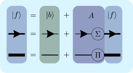
Figure 1: Relationship between linear system, Dyson equation and Bethe-Salpeter equation.

As from the original paper [15], BDMC can be viewed as trying to solve a self-consistent linear equation:

$$\ket{f}=\ket{b}+A\ket{f},$$ (1)

where $\ket{f}$ is an unknown vector, $\ket{b}$ is a given vector, and $A$ is a linear operator. Figure 1 provides the connection between (1) with either the Dyson equation or the Bethe-Salpeter equation [21]. Since either $\Sigma$ or $\Pi$ involves infinite terms of diagrams, the evaluation is carried out via a stochastic procedure up to a given number of terms. The evaluation of $A\ket{f}$, therefore, is stochastic, where the error is controlled by the number of Monte Carlo sampling. Prokof’ev and Svistunov in 2007 proposed an iterative method to solve for $\ket{f}$ in (1) under the stochastic setting, whose connection to conventional iterative algorithm in numerical linear algebra is not obvious from the first sight. As BDMC achieves success in many interacting systems and shows great promise, establishing a concrete understanding of the iterative method in a mathematical way is crucial for further improvement of the method, and potentially adapt the method to other applications.

In this note, we interpret the “magic” method proposed in [15] as a combination of two crucial steps. The first step replaces the original operator $A$ by a quadratic polynomial of $A$, $p(A)$, such that $p(0)=0$, $p(A)\succeq 0$ and potentially $\kappa\left(p(A)\right)\ll\kappa\left(A^{*}A\right)$, where “$A\succeq 0$” means that $A$ is a positive semidefinite matrix and $\kappa\left(A\right)$ denotes the condition number of matrix $A$. Here, “$p(0)=0$” guarantees the equality in (1), “$p(A)\succeq 0$” guarantees the convergence of the iterative method, and “$\kappa\left(p(A)\right)\ll\kappa\left(A^{*}A\right)$” enables faster convergence rate. Based on this understanding, we suggest another form of the quadratic polynomial such that the similar properties can be achieved for a wider range of $A$. In the second step, a fixed point iteration with adaptive stepsize is applied to (1) with $A$ being replaced by $p(A)$, and the corresponding update on $\ket{b}$. When $A$ is a Hermitian matrix, the second step can be viewed as a method of stochastic gradient descent. Hence, later in the note, we employ stochastic gradient descent methods from machine learning as alternative methods. All methods are tested on synthetic stochastic matrix $A$ instead of diagrams for real physical systems; those will be considered for future works.

In this note, we will provide mathematical understanding of the stochastic iterative method [15] in Section 2. Section 3 lists several alternative stochastic iterative methods. All the mentioned methods are tested and compared in Section 4. Finally, in Section 5, we conclude the note together with discussion of possible future works.

2 Numerical method of BDMC

Recall the fixed-point problem BDMC tries to solve:

$$\ket{f}=\ket{b}+A\ket{f}.$$ (2)

In the viewpoint of linear algebra, we rewrite the equation as

$$M\ket{f}=\ket{b},$$ (3)

where $M=I-A$, $I$ is the identity matrix of the same size as $A$. BDMC proposes replacements $\ket{b}\rightarrow\ket*{\widetilde{b}}=\ket{b}-\lambda A\ket{b}$ and $A\rightarrow\widetilde{A}=(1+\lambda)A-\lambda A^{2}$ to ensure the convergence of the iterative method, where $\lambda$ is a constant related to the spectrum of $A$. Then a simple fixed-point iteration is coupled with a special Nørlund means to solve (2) with $\widetilde{A}$ and $\ket*{\widetilde{b}}$. In the following subsections, we reinterpret the former as a preconditioning step and the latter as a stochastic gradient descent method with diminishing stepsize.

In the rest of this note, we would stick to linear algebra notations as in (3). Accordingly, we have $\ket*{\widetilde{b}}=(1-\lambda)\ket{b}+\lambda M\ket{b}$, $\widetilde{M}=I-\widetilde{A}=(1-\lambda)M+\lambda M^{2}$. Additionally, we follow the assumption as in [15] that $A$ is Hermitian, i.e., $A^{*}=A$. Therefore, both $M$ and $\widetilde{M}$ are Hermitian as well.

2.1 Preconditioning indefinite matrices

For almost all first-order iterative methods, positivity of $M$ is required for convergence. Methods that work for indefinite matrices, such as MINRES [13], GMRES [18], adopt some transforms of $M$, e.g., $M^{*}M$, $M^{2}$, to turn the matrix in the iterative method positive definite. Another important property of $M$ or $\widetilde{M}$ related to convergence rate is the condition number. In general, smaller condition number leads to faster convergence. However, treatment as $M^{*}M$ or $M^{2}$ squares the condition number which is undesirable in practice. In this section, we analyze the positivity of $\widetilde{M}$ and its condition number comparing to $\kappa\left(M^{2}\right)$.

Assume $M$ is an indefinite invertible matrix of size $n$ by $n$. According to the earlier assumption, $M$ is Hermitian. Let $M=Q\Lambda Q^{*}$ be the eigenvalue decomposition of $M$, where $Q$ is a unitary matrix of size $n$ by $n$, $\Lambda$ is a diagonal matrix with $M$’s eigenvalues, $\{m_{1},m_{2},\dots,m_{n}\}$, in decreasing order, i.e., $m_{1}\geq m_{2}\geq\cdots\geq m_{\ell}>0>m_{\ell+1}\geq\cdots\geq m_{n}$ for $1<\ell<n$. To simplify the presentation in the sequel, we introduce handy notations as, $L_{+}=\max_{1\leq i\leq n}m_{i}$, $L_{-}=\min_{1\leq i\leq n}m_{i}$, $\tau_{+}=\min_{m_{i}>0}m_{i}$, and $\tau_{-}=\max_{m_{i}<0}m_{i}$, which define the boundaries of the positive and negative spectrum of $M$.

$\widetilde{M}=(1-\lambda)M+\lambda M^{2}$ inherits the same eigenvectors as $M$. The eigenvalues of $\widetilde{M}$ are $\left\{(1-\lambda)m_{i}+\lambda m_{i}^{2}\right\}_{i=1}^{n}$. Denote the quadratic polynomial depending on parameter $\lambda$ as $p_{\lambda}(x)=\lambda x^{2}+(1-\lambda)x$. The eigenvalues of $\widetilde{M}$, therefore, are polynomial $p_{\lambda}(x)$ acting on the eigenvalues of $M$. $\widetilde{M}$ being a positive definite matrix is equivalent to $p_{\lambda}(m_{i})>0$ for all $m_{1},\dots,m_{n}$. Since $p_{\lambda}(x)$ is a quadratic polynomial with zero being one of its root, $p_{\lambda}(\tau_{-})>0$ and $p_{\lambda}(\tau_{+})>0$ imply that $\lambda>0$. At the same time, the second root of $p_{\lambda}(x)$, $\frac{\lambda-1}{\lambda}$, must lies in the interval $(\tau_{-},\tau_{+})$. Hence the equivalent condition for $\widetilde{M}$ being positive definite is that

$$\tau_{-}<\frac{\lambda-1}{\lambda}<\tau_{+}\Leftrightarrow\left\{\begin{array}[]{ll}\lambda>\frac{1}{1-\tau_{-}}\\ \lambda<\frac{1}{1-\tau_{+}}\quad\text{if }\tau_{+}<1\end{array}\right..$$ (4)

We now move on to the second concern, the condition number of $\widetilde{M}$ comparing to that of $M^{2}$. Using the notations above, the condition number of $M^{2}$ is

$$\kappa\left(M^{2}\right)=\frac{\max\left(L_{+}^{2},L_{-}^{2}\right)}{\min\left(\tau_{+}^{2},\tau_{-}^{2}\right)},$$

and the condition number of $\widetilde{M}$ is

$$\kappa_{\lambda}\bigl{(}\widetilde{M}\bigr{)}=\frac{\max\left(p_{\lambda}(L_{+}),p_{\lambda}(L_{-})\right)}{\min\left(p_{\lambda}(\tau_{+}),p_{\lambda}(\tau_{-})\right)}.$$ (5)

The optimal choice $\lambda^{*}=\operatorname*{arg\,min}_{\lambda\text{ satisfies}\eqref{eq:tM-psd-cond}}\kappa_{\lambda}\bigl{(}\widetilde{M}\bigr{)}$ is difficult to determine. On the other hand, a simple choice,

$$\widehat{\lambda}=\left\{\begin{array}[]{ll}\frac{1}{1-\tau_{+}-\tau_{-}}&\text{if }\tau_{+}+\tau_{-}<1-\frac{1}{C}\\ C&\text{if }\tau_{+}+\tau_{-}\geq 1-\frac{1}{C}\end{array}\right.$$

leads to

$$\min\left(p_{\widehat{\lambda}}(\tau_{+}),p_{\widehat{\lambda}}(\tau_{-})\right)=\left\{\begin{array}[]{ll}-\widehat{\lambda}\tau_{+}\tau_{-}&\text{if }\tau_{+}+\tau_{-}<1-\frac{1}{C}\\ \widehat{\lambda}\tau_{-}(\tau_{-}-1+\frac{1}{C})&\text{if }\tau_{+}+\tau_{-}\geq 1-\frac{1}{C}\end{array}\right.,$$

where $C$ is a sufficiently large constant. When $\absolutevalue{\tau_{-}}$ is orders of magnitude larger than $\tau_{+}$ and $\max\left(L_{+},L_{-}\right)\gg\absolutevalue{\tau_{-}}$, the condition number $\kappa_{\widehat{\lambda}}\bigl{(}\widetilde{M}\bigr{)}$ is roughly $\frac{\absolutevalue{\tau_{-}}}{\tau_{+}}$ times smaller than $\kappa\left(M^{2}\right)$. More extreme example is that when $\absolutevalue{\tau_{-}}\sim\absolutevalue{L_{-}}>L_{+}\gg\tau_{+}$, the condition number of $\widetilde{M}$ is roughly constant, $\kappa_{\widehat{\lambda}}\bigl{(}\widetilde{M}\bigr{)}=\order{1}$, whereas the condition number $\kappa\left(M^{2}\right)$ could be gigantic if the ratio $\absolutevalue{L_{-}}/\tau_{+}$ is gigantic. Figure 2 shows the comparison between $p_{\lambda}(M)$ and $M^{2}$. The largest eigenvalue of $M^{2}$ is obviously larger than that of $p_{\lambda}(M)$, and the smallest eigenvalue of $M^{2}$ is also smaller than that of $p_{\lambda}(M)$ (shown in the zoom-in subfigure). Therefore, in this case, the condition number of $M^{2}$ is much larger than that of $p_{\lambda}(M)$. However, when we swap the position of $\tau_{+}$ and $\tau_{-}$, e.g., $\tau_{+}$ is orders of magnitude larger than $\absolutevalue{\tau_{-}}$ and $\max\left(L_{+},L_{-}\right)\gg\tau_{+}$, the condition number $\kappa_{\widehat{\lambda}}\bigl{(}\widetilde{M}\bigr{)}$ could be of the same order as $\kappa\left(M^{2}\right)$ if $\absolutevalue{\tau_{-}}\sim 1$. The limitation comes from the restricted expression of $p_{\lambda}(x)$, where the second root must be smaller than one if $\lambda>0$.

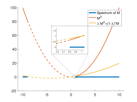
Figure 2: Two quadratic polynomials act on the spectrum of a matrix $M$ with $L_{-}=-10$, $\tau_{-}=-9$, $\tau_{+}=0.8$ and $L_{+}=10$.

In summary of the above analysis, we observe that the quadratic polynomial of the matrix, $p_{\lambda}(M)$ with a careful choice of $\lambda$, turns $M$ into a positive definite matrix. For a certain class of matrices, $p_{\lambda}(M)$ is much well-conditioned than the traditional technique $M^{2}$, which is favorable for the later iterative method. Furthermore, according to the choice of $\widehat{\lambda}$, the improvement of the condition number is more significant when $M$’s close-to-zero eigenvalues are tiled around zero.

Generic quadratic polynomial preconditioning. Inspired by the above analysis, we propose a more generic quadratic polynomial $p_{\delta}(x)=x^{2}-\delta x$ for preconditioning, where $\delta$ is a parameter playing the similar role as $\lambda$. By abuse of notation, $\widetilde{M}=p_{\delta}(M)$. Similar as before, $\widetilde{M}$ and $M$ share the same eigenvectors and the eigenvalues of $\widetilde{M}$ are $p_{\delta}(m_{i})=m_{i}^{2}-\delta m_{i}$. Since $\delta$ is the second root of $p_{\delta}(x)$, $\tau_{-}<\delta<\tau_{+}$ guarantees the positivity of $\widetilde{M}$. The definition of the condition number of $\widetilde{M}$ is as (5),

$$\kappa_{\delta}\bigl{(}\widetilde{M}\bigr{)}=\frac{\max\left(p_{\delta}(L_{+}),p_{\delta}(L_{-})\right)}{\min\left(p_{\delta}(\tau_{+}),p_{\delta}(\tau_{-})\right)}.$$ (6)

The optimal choice of $\delta$, $\delta^{*}=\operatorname*{arg\,min}_{\tau_{-}<\delta<\tau_{+}}\kappa_{\delta}\bigl{(}\widetilde{M}\bigr{)}$, is difficult to determine. We adopt the simple choice $\widehat{\delta}=\tau_{+}+\tau_{-}$, leading to

$$\min\left(p_{\widehat{\delta}}(\tau_{+}),p_{\widehat{\delta}}(\tau_{-})\right)=-\tau_{-}\tau_{+}.$$

The condition number $\kappa_{\widehat{\delta}}\bigl{(}\widetilde{M}\bigr{)}$ has similar behavior as $\kappa_{\widehat{\lambda}}\bigl{(}\widetilde{M}\bigr{)}$ when $\tau_{-}$ is away from zero and $\tau_{+}$ is close to zero. Different behavior appears when $\tau_{-}$ is closer to zero than $\tau_{+}$. When $\tau_{+}$ is orders of magnitude larger than $\absolutevalue{\tau_{-}}$ and $\max\left(L_{+},L_{-}\right)\gg\tau_{+}$, the condition number $\kappa_{\widehat{\delta}}\bigl{(}\widetilde{M}\bigr{)}$ is $\frac{\tau_{+}}{\absolutevalue{\tau_{-}}}$ times smaller than $\kappa\left(M^{2}\right)$. Therefore $p_{\delta}(x)$ has broader applicable range than $p_{\lambda}(x)$.  In Figure 3, we demonstrate the advantage of $p_{\widehat{\delta}}(M)$ over $p_{\widehat{\lambda}}(M)$ for some matrix $M$.

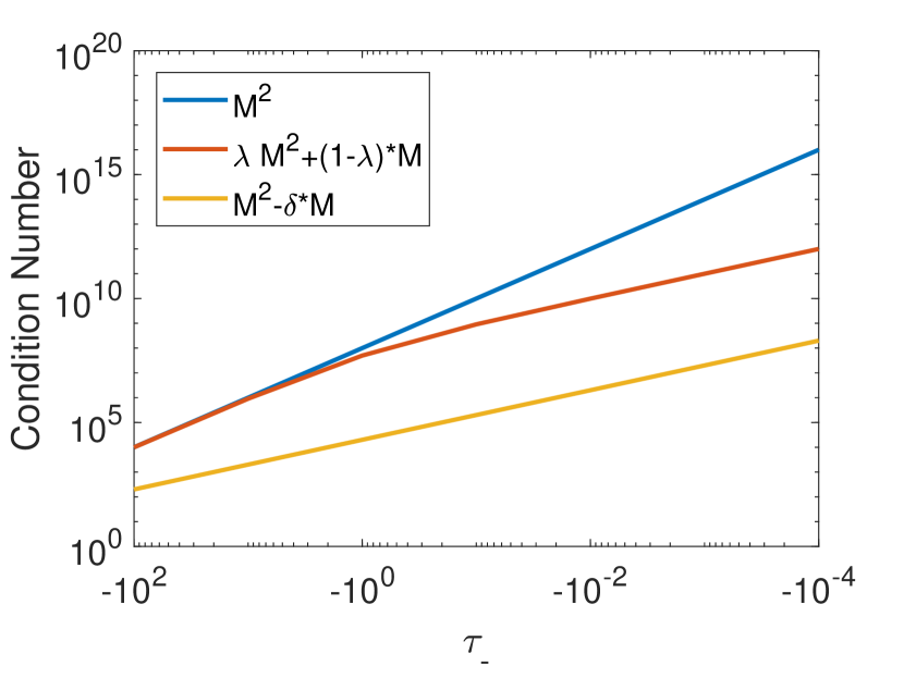
(a)

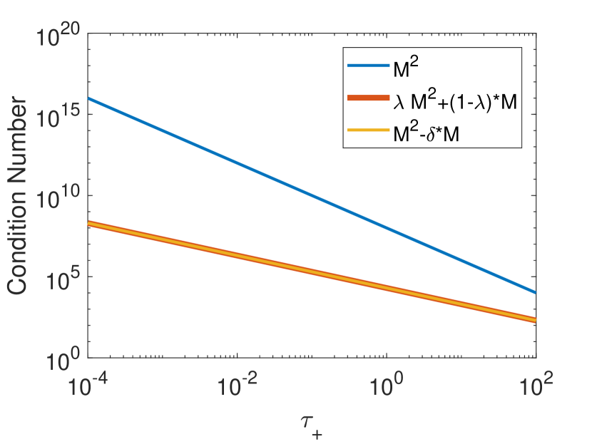
(b)

Figure 3: Condition number of a matrix $M$ with varying asymmetric spectrum. In both (a) and (b), the matrix $M$ has fixed $L_{+}=10^{4}$, $L_{-}=-10^{4}$. (a) fixes the smallest positive eigenvalue $\tau_{+}=10^{4}-1$ and varies $\tau_{-}$; (b) fixes the largest negative eigenvalue $\tau_{-}=-10^{4}+1$ and varies $\tau_{+}$.

Remark 2.1.

Both $p_{\widehat{\delta}}(M)$ and $p_{\widehat{\lambda}}(M)$ take advantage of the asymmetry of the spectrum of $M$. When the spectrum of $M$ is symmetric around the origin, i.e., $\tau_{+}=\tau_{-}$ and $L_{+}=L_{-}$, the choice of either $p_{\widehat{\delta}}(M)$ or $p_{\widehat{\lambda}}(M)$ falls back to $M^{2}$, which has the same condition number as $M^{*}M$.

2.2 BDMC Iterative method

In terms of matrix $M$ as in (3), the two-step iterative method in [15] can be written as

$$\begin{array}[]{ll}\text{Step 1:}&\ket{\widetilde{f}_{k+1}}=\ket{b}+(I-M)\ket{f_{k}}\\ \text{Step 2:}&\ket{f_{k+1}}=\cfrac{\sum_{j=1}^{k+1}j^{t}\ket{\widetilde{f}_{j}}}{\sum_{j=1}^{k+1}j^{t}}\end{array}$$ (7)

where $t>-1$ is a fixed parameter.  Step 1 is a fixed-point iteration and Step 2 is a special Nørlund mean with sequence $\{j^{t}\}$. Let $S_{k}=\sum_{j=1}^{k}j^{t}$. We could merge two steps into a single step,

$$\ket{f_{k+1}}=\frac{1}{S_{k+1}}\ket{f_{k}}+\frac{(k+1)^{t}}{S_{k+1}}\ket{\widetilde{f}_{k+1}}=\ket{f_{k}}-\frac{(k+1)^{t}}{S_{k+1}}\left(M\ket{f_{k}}-\ket{b}\right).$$ (8)

For Hermitian positive definite matrix $M$, (8) is a gradient descent method for the objective function $\expectationvalue{M}{f}-\bra{b}\ket{f}$ with special stepsize $\alpha_{k}=\frac{(k+1)^{t}}{S_{k+1}}$. Such a stepsize asymptotically behaves as

$$\alpha_{k}\asymp\frac{t+1}{k+1}\quad(k\rightarrow+\infty).$$ (9)

In fact, the simpler stepsize choice as (9) is widely used in the stochastic gradient descent literature. We would denote $\beta=t+1$ in the following note. The convergence analysis of the iterative method,

$$\ket{f_{k+1}}=\ket{f_{k}}-\frac{\beta}{k+1}\left(M\ket{f_{k}}-\ket{b}\right)$$ (10)

for both deterministic and stochastic $M$ are listed in the next section.

2.3 Convergence Analysis

Let us now turn to the convergence analysis of iterative algorithms (8) and (10). Compared the two, the analysis of (10) would be cleaner due to its simpler choice of stepsize. In [15], Prokof’ev and Svistunov provide asymptotic behavior for $\ket{\delta_{k}}=\ket{f_{k}}-\ket{f^{*}}$, which is the difference between step $k$ result $\ket{f_{k}}$ and the underlying truth $\ket{f^{*}}=M^{-1}\ket{b}$. When $k$ approaches $+\infty$, $\ket{\delta_{k}}$ behaves as

$$\ket{\delta_{k}}\asymp e^{-\beta M\log{k}}\ket{\delta_{1}},$$ (11)

where $\ket{\delta_{1}}=\ket{f_{1}}-\ket{f^{*}}$ and $\ket{f_{1}}$ is the initial guess. Since $M$ is a positive definite matrix and $\beta>0$, $\ket{\delta_{k}}\rightarrow\ket{0}$ as $k\rightarrow+\infty$. The same asymptotic analysis holds for stepsize (9) as well. According to (11), the slowest converging component behaves as $e^{-\beta\tau_{+}\log{k}}$, where $\tau_{+}$ is the smallest eigenvalue of $M$. Careful study of the contraction property of the iterative method shows that either $\beta$ or the number of non-contraction steps is related to the largest eigenvalue $L_{+}$ of $M$. Overall, the smaller condition number of $M$ leads to the faster convergence.

Remark 2.2.

Based on the above asymptotics, it was suggested in [15] the choice of very large $\beta$. In that case, for sufficiently large $k$, the asymptotic rate (11) is achieved. This is however only part of the story, as for the iterative method, we are not just interested in asymptotic convergence, the actual decay of error after finite number of steps is more important. Indeed as we will see in Corollary 2.5, the hidden prefactor in (11) depends on $\beta$. In particular, the asymptotic analysis fails if $t$ is set as $+\infty$ in the iterative method (8).

Moreover, the asymptotic analysis in (11) only holds for noise-free matrix $M$. In the stochastic setting, i.e., each evaluation of $M\ket{f}$ involves a stochastic error, we will see in Theorem 2.4 that the expected error is dominated by the stochastic error part. The choice of large $\beta$ does not impact the convergence rate of the iterative method but enlarges the prefactor. Therefore, choosing large $\beta$ in the stochastic setting actually has negative influence on the convergence.

The previous asymptotic analysis holds for deterministic matrix $M$. For stochastic matrix vector multiplication, the analysis is carried out with assumptions on the bias and variance, we present one possible convergence result below, following Theorem 4.7 in the review article [3].

Let $G(\ket{f})=\expectationvalue{M}{f}-\bra{b}\ket{f}$ for Hermitian positive definite matrix $M$. The gradient of $G(\ket{f})$ is $\nabla{G(\ket{f})}=M\ket{f}-\ket{b}$. Hence, both (8) and (10) are gradient descent methods applied to $G(\ket{f})$. In order to distinguish between the deterministic gradient and stochastic gradient, we denote the stochastic one as $g(\ket{f},\xi)=M_{\xi}\ket{f}-\ket{b}$, where $\xi$ is a random variable.

Assumption 2.3.

The objective function and stochastic gradient method as (10) satisfies the following:

1. There exist scalars $\mu_{G}\geq\mu>0$ such that, for all $k\in\mathbb{N}$,

   $$\begin{split}&\nabla{G(\ket{f_{k}})}^{*}\mathbb{E}\left[g(\ket{f_{k}},\xi_{k})\right]\geq\mu\norm{\nabla{G(\ket{f_{k}})}}_{2}^{2},\quad\text{and}\\ &\norm{\mathbb{E}\left[g(\ket{f_{k}},\xi_{k})\right]}_{2}\leq\mu_{G}\norm{\nabla{G(\ket{f_{k}})}}_{2}.\end{split}$$

2. There exist scalars $W\geq 0$ and $W_{V}\geq 0$ such that, for all $k\in\mathbb{N}$,

   $$\mathbb{V}\left[g(\ket{f_{k}},\xi_{k})\right]=\mathbb{E}\left[\norm{g(\ket{f_{k}},\xi_{k})}_{2}^{2}\right]-\norm{\mathbb{E}\left[g(\ket{f_{k}},\xi_{k})\right]}_{2}^{2}\leq W+W_{V}\norm{\nabla{G(\ket{f_{k}})}}_{2}^{2}.$$

Assumption 2.3 follows Assumption 4.3 in [3]. When $g(\ket{f_{k}},\xi_{k})$ is an unbiased estimator of $\nabla{G(\ket{f_{k}})}$, both $\mu_{G}$ and $\mu$ are one. We recall the notations $\tau=\tau_{+}$ and $L=L_{+}$ as the smallest and largest eigenvalue of $M$ respectively. Moreover, we denote $W_{G}=W_{V}+\mu_{G}^{2}$.

Theorem 2.4.

Under Assumption 2.3, suppose that the stochastic gradient method is run with a stepsize sequence such that for all $k\in\mathbb{N}$,

$$\alpha_{k}=\frac{\beta}{\gamma+k},\quad\beta>\frac{1}{\tau\mu},\quad\text{and }\gamma>0\quad\text{such that }\alpha_{1}\leq\frac{\mu}{LW_{G}}.$$

Then, for all $k\in\mathbb{N}$, the expected optimality gap satisfies

$$\mathbb{E}\left[G(\ket{f_{k}})-G_{*}\right]\leq\frac{1}{(\gamma+k)^{\beta\tau\mu}}\left(G(\ket{f_{1}})-G_{*}\right)(\gamma+1)^{\beta\tau\mu}+\frac{1}{\gamma+k}\frac{\beta^{2}LW}{\beta\tau\mu-1}$$ (12)

where $G_{*}=\inf_{\ket{f}}G(\ket{f})$.

Proof.

Starting from (4.23) in [3], we have,

$$\mathbb{E}\left[G(\ket{f_{k+1}})\right]-G_{*}\leq(1-\alpha_{k}\tau\mu)\left(\mathbb{E}\left[G(\ket{f_{k}})\right]-G_{*}\right)+\frac{1}{2}\alpha_{k}^{2}LW.$$ (13)

Equation (12) holds for $k=1$. Then assuming (12) is true for $k$, it follows from (13) that, ($\widehat{k}=\gamma+k$),

$$\begin{split}\mathbb{E}\left[G_{k+1}\right]-G_{*}\leq&\left(1-\frac{\beta\tau\mu}{\widehat{k}}\right)\widehat{k}{}^{-\beta\tau\mu}\left(G(\ket{f_{1}})-G_{*}\right)(\gamma+1)^{\beta\tau\mu}\\ &+\left(1-\frac{\beta\tau\mu}{\widehat{k}}\right)\frac{1}{\widehat{k}}\frac{\beta^{2}LW}{\beta\tau\mu-1}+\frac{1}{2}\frac{\beta^{2}}{\widehat{k}{}^{2}}LW\\ \leq&\frac{1}{(\widehat{k}+1)^{\beta\tau\mu}}\left(G(\ket{f_{1}})-G_{*}\right)(\gamma+1)^{\beta\tau\mu}+\frac{1}{\widehat{k}+1}\frac{\beta^{2}LW}{\beta\tau\mu-1}\end{split}$$

where the last inequality dues to Taylor expansion of $(\widehat{k}+1)^{-\beta\tau\mu}$ at $\widehat{k}$ and $\frac{\widehat{k}-1}{\widehat{k}{}^{2}}<\frac{1}{\widehat{k}+1}$. ∎

Theorem 2.4 now split the bound into the convergence of the initial error and stochastic error. Due to the assumption $\beta>\frac{1}{\tau\mu}$, the expected optimality gap is dominated by the stochastic error, which behaves as $O(\frac{1}{\gamma+k})$. At the same time, both the prefactor $\frac{\beta^{2}LW}{\beta\tau\mu-1}$ and the parameter of initial step size $\gamma\geq\frac{LW_{G}}{\tau\mu^{2}}-1$ relies on the condition number of $M$, i.e., $\frac{L}{\tau}$. Therefore, the smaller condition number of $M$ leads to the faster convergence in stochastic gradient descent method. A direct corollary can be derived for non-stochastic gradient descent method, where $\mu=\mu_{G}=1,W=0,W_{G}=1$.

Corollary 2.5.

Suppose the gradient descent method is run with a stepsize sequence such that, for all $k\in\mathbb{N}$,

$$\alpha_{k}=\frac{\beta}{\gamma+k},\quad\text{and }\gamma>0\quad\text{such that }\alpha_{1}\leq\frac{1}{L}.$$

Then, for all $k\in\mathbb{N}$, the optimality gap satisfies

$$G(\ket{f_{k}})-G_{*}\leq\frac{1}{(\gamma+k)^{\beta\tau}}\left(G(\ket{f_{1}})-G_{*}\right)(\gamma+1)^{\beta\tau}.$$

Corollary 2.5 coincides with (11). The impact of the condition number of $M$ to the convergence is more significant in the non-stochastic gradient descent method. The constant $(\gamma+1)^{\beta\tau}$ and parameter $\gamma$ are influenced by the condition number in a similar way as the stochastic one. The rate of the convergence of the non-stochastic gradient descent method is also impacted by the smallest eigenvalue of $M$. In general, the larger of $\tau$ leads to faster convergence rate of the gradient descent method. Such an argument agrees with the asymptotic analysis of (11).

3 Alternative stochastic iterative methods

Gradient descent method with stochastic gradient is widely explored in many areas. Especially, machine learning researchers established many variant stochastic gradient descent methods to minimize the loss function in a big data setting. The raise of deep learning further accelerates the development of stochastic gradient descent methods. In these context, many loss functions are non-convex functions. Stochastic gradient descent methods, without accessing full gradient at each step, samples a few components of the full gradient and move along the sampled gradient direction. This strategy reduces the computational cost each step and potentially avoids many local minima. The problem BDMC addresses, in contrast with deep learning, has a quadratic convex objective function. On the other hand, the gradient of the objective function in BDMC can only be accessed via a Monte Carlo procedure. The underlying true gradient is unknown. Here we would like to compare BDMC with a few well-established stochastic gradient descent methods from machine learning literature. The cross-fertilization between machine learning and computational physics is rather natural since both are dealing with high dimensional problems. In particular, diagrammatic summation methods like BDMC could potentially benefit from other stochastic iterative methods to either improve convergence or allow larger Monte Carlo error.

3.1 Heavy ball method

The heavy ball method [14] adds a momentum term to the gradient descent method,

$$\ket{f_{k+1}}=\ket{f_{k}}-\alpha(M\ket{f_{k}}-\ket{b})+\beta\left(\ket{f_{k}}-\ket{f_{k-1}}\right),$$ (14)

where $\alpha$ is the stepsize and $\beta$ is the weight for momentum. Heavy ball method actually has the same convergence rate as the gradient descent method. Unlike gradient descent method which depends on the condition number of $M$, the heavy ball method depends on the square root of the condition number of $M$. Such a property is attractive when $M$ is ill-conditioned. However, due to the momentum, the heavy ball method is not strictly decreasing, i.e., $G(\ket{f_{k+1}})$ is not necessarily smaller than $G(\ket{f_{k}})$.

3.2 Stochastic Barzilai-Borwein method

In 1988, Barzilai and Borwein proposed a two-point step size gradient method [2], which is inspired by the secant equation underlying quasi-Newton methods. The stochastic version of the Barzilai and Borwein method (sBB) [19], instead of updating the stepsize every iteration with the difference of stochastic gradients, updates the stepsize every $m$ iteration with the difference of aggregated gradients. The detailed iteration is as follows,

$$\begin{split}&\alpha_{k}=\left\{\begin{array}[]{ll}\alpha_{k-1}&\text{if }k\not\equiv 0\mod m\\ \frac{1}{m}\frac{\bra{\Delta_{k}^{m}f}\ket{\Delta_{k}^{m}f}}{\bra{\Delta_{k}^{m}f}\ket{\Delta_{k}^{m}g}}&\text{if }k\equiv 0\mod m\\ \end{array}\right.\\ &\ket{f_{k+1}}=\ket{f_{k}}-\alpha_{k}\nabla{G(\ket{f_{k}})}\\ &\ket{g_{k+1}}=\beta\nabla{G(\ket{f_{k}})}+(1-\beta)\ket{g_{k}}\end{split}$$ (15)

where $\ket{\Delta_{k}^{m}f}=\ket{f_{k}}-\ket{f_{k-m}}$ and $\ket{\Delta_{k}g}=\ket{g_{k}}-\ket{g_{k-m}}$. $\beta$ is the weight for momentum and $m$ is the updating frequency. Notice that in [19], a smoothing technique is suggested for the stepsize, which is a technique enforce diminishing stepsize. According to our tests, this technique is crucial for convergence when the gradient is noisy. Therefore, our implementation of sBB adopts the smoothing technique.

3.3 AdaGrad method

AdaGrad method [5] approximates the Hessian of $G$ by a diagonal matrix, and sets the stepsize in the gradient method as the inverse of the diagonal approximation. The iteration of AdaGrad method is

$$\ket{f_{k+1}}=\ket{f_{k}}-\alpha\text{diag}\left(\Gamma_{k}\right)^{-1/2}\nabla{G(\ket{f_{k}})},$$ (16)

where $\Gamma_{k}=\sum_{i=1}^{k}\left(\nabla{G(\ket{f_{k}})}\right)^{2}$ and the square is an entry-wise operation, $\alpha$ is a parameter. Since the computational costs for both the inverse of the square root of a diagonal matrix and the diagonal matrix vector multiplication are the same as generating the gradient vector. Therefore, such a choice of stepsize only increase the computational cost by a small constant, while the convergence could be accelerate for stochastic gradients.

3.4 ADAM method

ADAM method [8] is a upgraded version of AdaGrad method. Instead of using raw gradient $\nabla{G(\ket{f_{k}})}$ and $\Gamma_{k}$ as in (16), ADAM method adds momentum parts for both and correct the biases. The calculation of its stepsize is more complicated than all pre-mentioned methods. We summarize the calculation as follows,

$$\begin{split}&\ket{g_{k+1}}=\nabla{G(\ket{f_{k}})}\\ &\ket{m_{k+1}}=\beta_{1}\ket{m_{k}}+(1-\beta_{1})\ket{g_{k+1}}~{}\text{[Update biased first moment]}\\ &\ket{v_{k+1}}=\beta_{2}\ket{v_{k}}+(1-\beta_{2})\ket{g_{k+1}}^{2}~{}\text{[Update biased second moment]}\\ &\ket{\widehat{m}{}_{k+1}}=\ket{m_{k+1}}/(1-\beta_{1}^{k+1})~{}\text{[Correct biased first moment]}\\ &\ket{\widehat{v}{}_{k+1}}=\ket{v_{k+1}}/(1-\beta_{2}^{k+1})~{}\text{[Correct biased second moment]}\\ &\ket{f_{k+1}}=\ket{f_{k}}-\alpha\widehat{m}{}_{k+1}/(\sqrt{\widehat{v}{}_{k+1}}+\epsilon)\\ \end{split}$$ (17)

with initial first moment vector $\ket{m_{1}}=\ket{0}$ and second moment vector $\ket{v_{1}}=\ket{0}$, where $\beta_{1}$ and $\beta_{2}$ are weights for the first and second moment respectively, $\alpha$ is a parameter. These initial first and second moment are crucial for the bias correction parts. Although the iterative scheme looks much more complicated than before, the computational cost is about 2-3 times as much as that of AdaGrad method.

4 Numerical Results

This section focus on testing the performances of different gradient descent methods mentioned in Section 2.2 and Section 3. The power of the preconditioning technique has been illustrated in Figure 3, and we would not retest it here. The algorithms of different gradient descent methods are implemented in MATLAB 2017b and the results reported here are obtained on a MacBook Pro with 2.3 GHz Intel Core i7 and 8 GB memory.

For simplicity, we will use the shorten name as in Table 1 instead of the original full name. The accuracy of all iterative methods is measured against the underlying true solution $\ket{f^{*}}$ as,

$$e_{k}^{rel}=\frac{\norm{\ket{f_{k}}-\ket{f^{*}}}}{\norm{f^{*}}},$$ (18)

where $\ket{f_{k}}$ is the solution at $k$th step and $e_{k}^{rel}$ is called the relative error at $k$th step.

Short Name	Full Name	Scheme
GD	Gradient descent method
BDMC	Bold Diagrammatic Monte Carlo method	Section 2.2 (7)
BDMC2	Bold Diagrammatic Monte Carlo method	Section 2.2 (10)
HB	Heavy ball method	Section 3.1
sBB	Stochastic Barzilai-Borwein method	Section 3.2
AdaGrad	Adaptive gradient method	Section 3.3
ADAM	Adaptive moment estimation method	Section 3.4

Table 1: Name convention for iterative methods.

One example is to simulate the DMC by noisy symmetric positive definite matrices $M$ of size 100 by 100. We first generate the simulating system as follows,

$$M=Q\begin{bmatrix}1&&&\\ &2&&\\ &&\ddots&\\ &&&100\end{bmatrix}Q^{*},$$ (19)

where $Q$ is a random unitary matrix. Then a underlying true solution $\ket{f^{*}}$ is generated from normal distribution. The vector $\ket{b}$, therefore, is the multiplication of $M$ and $\ket{f^{*}}$, i.e., $\ket{b}=M\ket{f^{*}}$. In order to simulate the uncertainty of the DMC, we added noise to each entry of $M\ket{f}$, i.e.,

$$g(\ket{f},\xi)=M\ket{f}-\ket{b}+\epsilon\ket{\xi},$$ (20)

where $\ket{\xi}$ is a random vector with each entry drawn from standard normal distribution and $\epsilon$ is the noise level.

	GD	BDMC	BDMC2	HB		sBB		AdaGrad	ADAM
$\epsilon$	$\alpha$	$t$	$\beta$	$\alpha$	$\beta$	$m$	$\beta$	$\alpha$	$\alpha$	$\beta_{1}$	$\beta_{2}$
$0.01$	$0.005$	$-0.6$	$0.4$	$0.01$	$0.6$	$50$	$0.9$	$0.9$	$0.1$	$0.99$	$0.999$
$0.1$	$0.001$	$-0.6$	$0.4$	$0.001$	$0.6$	$50$	$0.4$	$0.4$	$0.01$	$0.99$	$0.999$
$1$	$0.0005$	$-0.5$	$0.5$	$0.0005$	$0.6$	$30$	$0.5$	$0.2$	$0.001$	$0.99$	$0.999$
$10$	$0.0003$	$-0.5$	$0.5$	$0.0001$	$0.6$	$40$	$0.5$	$0.2$	$0.002$	$0.99$	$0.999$
$100$	$0.00008$	$-0.4$	$0.5$	$0.00005$	$0.6$	$50$	$0.4$	$0.2$	$0.002$	$0.99$	$0.999$

Table 2: “Close-to-optimal” parameters of iterative methods for the first example.

Each different gradient descent method in Section 2.2 and Section 3 has some parameters in common, maximum number of iteration is $10000$, convergence tolerance is $10^{-6}$, initial guess $\ket{f_{1}}$ is a random vector with entry drawn from standard normal distribution (except that ADAM always starts from $\ket{0}$). Besides these common parameters, these methods have their own parameters requiring tuning. For each method, we tried different settings and summarize the close-to-optimal parameter in Table 2 up to one significant digits. “Close-to-optimal” is in the sense that the averaged relative error $\frac{\norm{\ket{f_{10000}}-\ket{f^{*}}}}{\norm{\ket{f^{*}}}}$ of 10 runs is minimized.

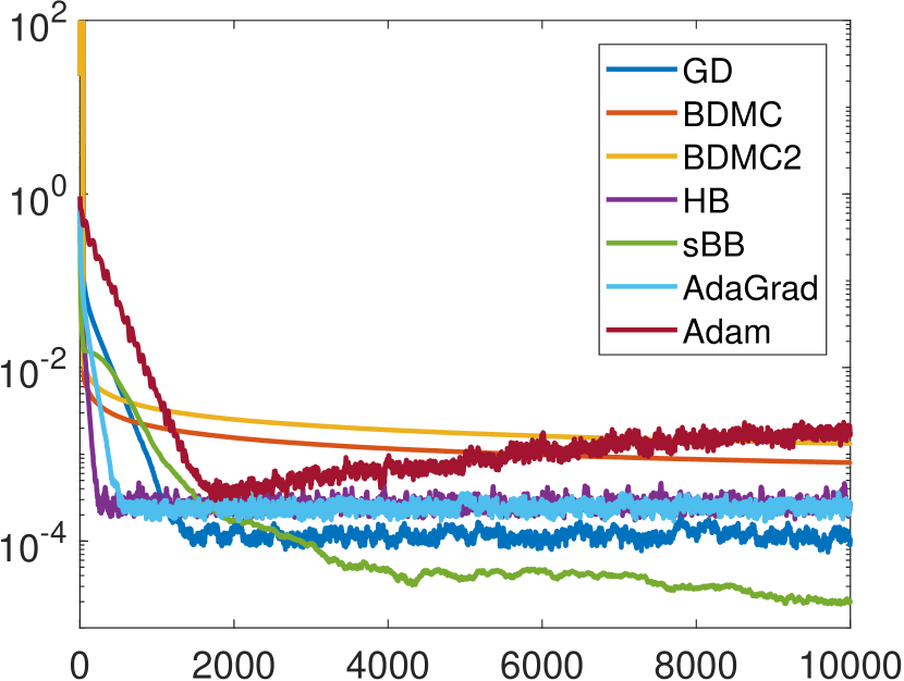
(a) $\epsilon=0.01$

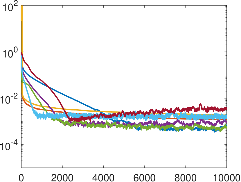
(b) $\epsilon=0.1$

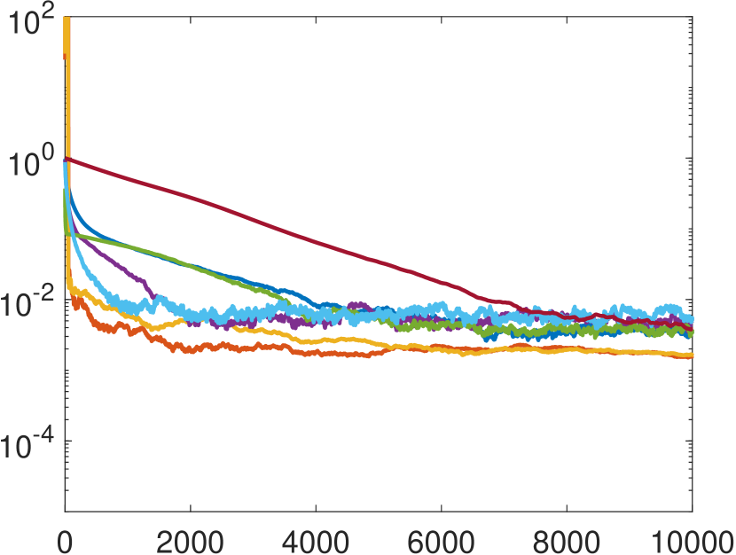
(c) $\epsilon=1$

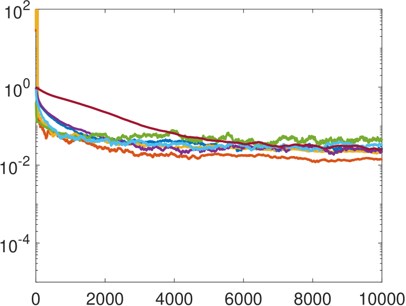
(d) $\epsilon=10$

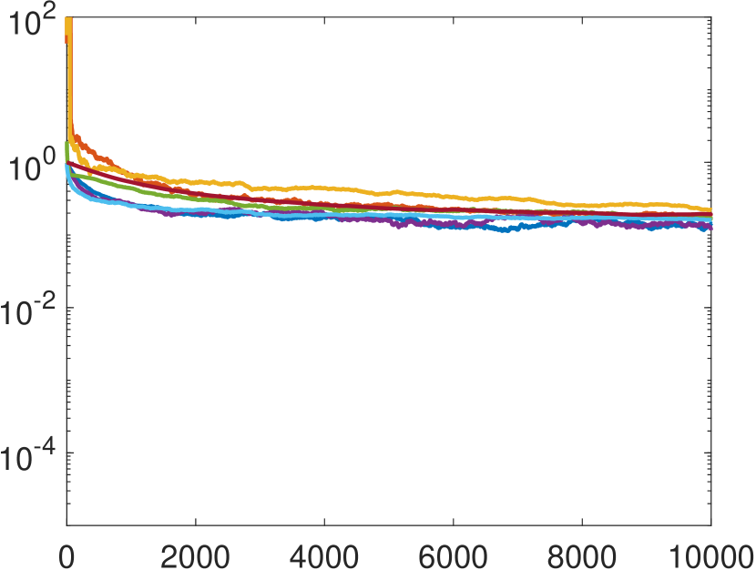
(e) $\epsilon=100$

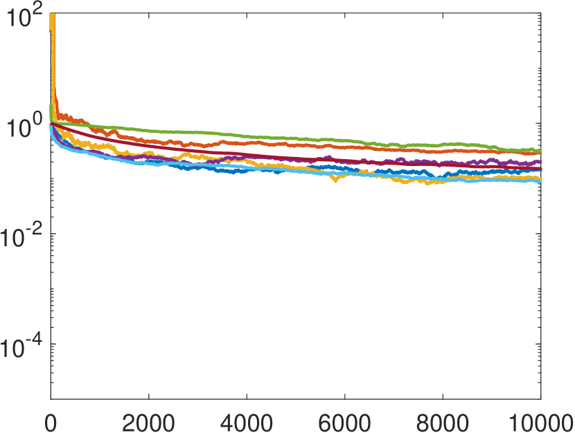
(f) $\epsilon=100$

Figure 4: Convergence results for different methods and different noise level. For all subfigures, $y$-axis denotes the relative error as in (18) and $x$-axis denotes the iteration number. The legends for (b) - (f) are the same as that in (a).

Figure 4 illustrates the performance of different stochastic gradient descent methods with different levels of noise in the gradient. According to Figure 4 (a) and (b), which correspond to low noise cases, the stochastic Barzilai-Borwein method outperforms other methods. Although it is not the best method in the first 2000 iterations, it achieves the best relative error when the iteration number getting larger. In these low noise cases, BDMC and BDMC2 do not perform well comparing to other methods. While, in the medium noise cases (see Figure 4 (c) and (d)), BDMC and BDMC2 are the best methods among all. They outperform other methods from the very beginning of the iterations. Based on our numerical tests, Figure 4 (a), (b), (c) and (d) are relatively robust with respect to different runs of the algorithms. However, as the noise level being close to the largest eigenvalue of $M$, the test results are no longer robust. The ranking of the methods shifts randomly. For example, Figure 4 (e) and (f) are two runs of the methods at the same noise level $\epsilon=100$. In (e), BDMC is the worst method, whereas in (f) it is one of the best. Therefore, conclusion of the ranking of the methods cannot be made here for the high noise level case.

We also would like to raise one concern about the BDMC and BDMC2 method. For both of them, the relative errors “blow up” in the first few iterations and quickly drop down to a reasonable level. And the peaks of the “blow-ups” could be as large as $10^{10}$ for the example here. These peaks are also related to the condition number of the original matrix $M$. The worse of the condition number of $M$, the higher of the peak. At the same time, the parameter $t$ must be tuned to close to $-1$ ($\beta$ in BDMC2 be tuned to close to $0$) to enable the drop-down behavior and achieve convergence.

The last point is about the sensitivity of the parameters. The parameters of gradient descent method and heavy ball method are the most sensitive ones, i.e., small change in the parameters would result huge performance difference. On the other side, the parameters in the stochastic Barzilai-Borwein method and AdaGrad method are the least sensitive ones. Although in Table 2, their parameters vary a lot, but many other choices of their parameters actually show similar convergence behavior. Therefore, these two methods are easier to use in practice.

5 Conclusion

This note provides mathematical understanding of the original BDMC method in [15]. The two parts in the BDMC method are interpreted as the preconditioning part and stochastic iterative part. In the preconditioning part, a quadratic polynomial of the matrix, $p_{\widehat{\lambda}}(M)$, turns an indefinite matrix into a positive definite matrix and the corresponding condition number could potentially be orders of magnitudes smaller than the traditional preconditioning technique, $M^{2}$. In addition to $p_{\widehat{\lambda}}(M)$, we propose another quadratic polynomial $p_{\widehat{\delta}}(M)$ which has the same performance on some matrices and achieves better performance on another big group of matrices. For the second part, the stochastic iterative part, we rewrite the original multi-step BDMC method as a gradient descent method with diminishing step size, (8). Asymptotically, the complicated stepsize can be replaced by (10). The choices of both stepsizes behave similar on all numerical examples we have tested. Due to the DMC procedure involved in the evaluation of the matrix, the BDMC iterative method is actually a stochastic gradient descent method on quadratic objective function. Naturally, we introduce a few stochastic gradient descent methods from machine learning and deep learning, which are originally designed for non-convex objective functions. All these stochastic gradient descent methods are tested on a simulated toy example with different level of noises. In the small noise levels, stochastic Barzilai-Borwein shows great power over other method. For medium noise level close to the smallest eigenvalue of the matrix, BDMC methods (with two choices of stepsize) outperform other methods. When the noise level is as large as the largest eigenvalue of the matrix, the conclusion for the performance of methods is unclear.

At this point, the new preconditioning technique and variant stochastic gradient descent methods are only tested on simulated matrices with noise. In the future, we would like to apply all these techniques and methods to the actual interacting systems using bold diagrammatic Monte Carlo method.

Acknowledgments. This work is partially supported by the National Science Foundation under awards OAC-1450280 and DMS-1454939. We thank Lexing Ying for interesting discussions regards the BDMC method.

References

- [1] B. M. Austin, D. Y. Zubarev, and W. A. Lester Jr. Qunatum Monte Carlo and related approaches. Chem. Rev., 112:263–288, 2012.
- [2] J. Barzilai and J. M. Borwein. Two-point step size gradient methods. IMA J. Numer. Anal., 8(1):141–148, jan 1988.
- [3] L. Bottou, F. E. Curtis, and J. Nocedal. Optimization methods for large-scale machine learning. Technical report, jun 2016.
- [4] D. M. Ceperley. An overview of quantum Monte Carlo methods. Rev. Mineral. Geochem., 71:129–135, 2010.
- [5] J. Duchi, E. Hazan, and Y. Singer. Adaptive subgradient methods for online learning and stochastic optimization. J. Mach. Learn. Res., 12:2121–2159, 2011.
- [6] A. L. Fetter and J. D. Walecka. Quantum theory of many-particle systems. Dover, 2003.
- [7] W. M. C. Foulkes, L. Mitas, R. J. Needs, and G. Rajagopal. Quantum Monte Carlo simulations of solids. Rev. Mod. Phys., 73:33–83, 2001.
- [8] D. P. Kingma and J. Ba. Adam: A method for stochastic optimization. In 3rd Int. Conf. Learn. Represent., San Diego, dec 2015.
- [9] J. Kolorenc and L. Mitas. Applications of quantum Monte Carlo methods in condensed systems. Rep. Prog. Phys., 4:026502, 2011.
- [10] S. A. Kulagin, N. V. Prokof’ev, O. A. Starykh, B. V. Svistunov, and C. N. Varney. Bold diagrammatic Monte Carlo method applied to Fermionized frustrated spins. Phys. Rev. Lett., 110(7):070601, feb 2013.
- [11] J. P. F. LeBlanc, A. E. Antipov, F. Becca, I. W. Bulik, G. K.-L. Chan, C.-M. Chung, Y. Deng, M. Ferrero, T. M. Henderson, C. A. Jiménez-Hoyos, E. Kozik, X.-W. Liu, A. J. Millis, N. V. Prokof’ev, M. Qin, G. E. Scuseria, H. Shi, B. V. Svistunov, L. F. Tocchio, I. S. Tupitsyn, S. R. White, S. Zhang, B.-X. Zheng, Z. Zhu, and E. Gull. Solutions of the two-dimensional Hubbard model: Benchmarks and results from a wide range of numerical algorithms. Phys. Rev. X, 5:041041, 2015.
- [12] R. D. Mattuck. A guide to Feynman diagrams in the many-body problem: second edition. Dover, 1992.
- [13] C. C. Paige and M. A. Saunders. Solution of sparse indefinite systems of linear equations. SIAM J. Numer. Anal., 12(4):617–629, sep 1975.
- [14] B. T. Polyak. Some methods of speeding up the convergence of iteration methods. USSR Comput. Math. Math. Phys., 4(5):1–17, jan 1964.
- [15] N. V. Prokof’ev and B. V. Svistunov. Bold diagrammatic Monte Carlo technique: When the sign problem is welcome. Phys. Rev. Lett., 99(25):250201, 2007.
- [16] N. V. Prokof’ev and B. V. Svistunov. Bold diagrammatic Monte Carlo: A generic sign-problem tolerant technique for polaron models and possibly interacting many-body problems. Phys. Rev. B, 77(12):125101, 2008.
- [17] N. V. Prokof’ev and B. V. Svistunov. Fermi-polaron problem: Diagrammatic Monte Carlo method for divergent sign-alternating series. Phys. Rev. B, 77(2):020408, jan 2008.
- [18] Y. Saad and M. H. Schultz. GMRES: A generalized minimal residual algorithm for solving nonsymmetric linear systems. SIAM J. Sci. Stat. Comput., 7(3):856–869, jul 1986.
- [19] C. Tan, S. Ma, Y.-H. Dai, and Y. Qian. Barzilai-Borwein step size for stochastic gradient descent. In D. D. Lee, M. Sugiyama, U. V. Luxburg, I. Guyon, and R. Garnett, editors, Adv. Neural Inf. Process. Syst. 29, pages 685–693. Curran Associates, Inc., 2016.
- [20] K. Van Houcke, E. Kozik, N. Prokof’ev, and B. Svistunov. Diagrammatic Monte Carlo. In D. P. Laudan, S. P. Lewis, and H. B. Schuttler, editors, Computer Simulation Studies in Condesed Matter Physics XXI. Springer, 2008.
- [21] K. Van Houcke, F. Werner, E. Kozik, N. V. Prokof’ev, B. V. Svistunov, M. J. H. Ku, A. T. Sommer, L. W. Cheuk, A. Schirotzek, and M. W. Zwierlein. Feynman diagrams versus Fermi-gas Feynman emulator. Nat. Phys., 8(5):366–370, 2012.