The GALEX/$\mathrm{S^{4}G}$ surface brightness and color profiles catalog - I. Surface photometry and color gradients of galaxies.

Abstract

We present new, spatially resolved, surface photometry in FUV and NUV from images obtained by the Galaxy Evolution Explorer (GALEX), and IRAC1 (3.6 $\mu$m) photometry from the Spitzer Survey of Stellar Structure in Galaxies ($\mathrm{S^{4}G}$) (Sheth et al., 2010). We analyze the radial surface brightness profiles $\mu_{FUV}$, $\mu_{NUV}$, and $\mu_{[3.6]}$, as well as the radial profiles of (FUV $-$ NUV), (NUV $-$ [3.6]), and (FUV $-$ [3.6]) colors in 1931 nearby galaxies (z $<$ 0.01). The analysis of the 3.6 $\mu$m surface brightness profiles also allows us to separate the bulge and disk components in a quasi-automatic way, and to compare their light and color distribution with those predicted by the chemo-spectrophotometric models for the evolution of galaxy disks of Boissier & Prantzos (2000). The exponential disk component is best isolated by setting an inner radial cutoff and an upper surface brightness limit in stellar mass surface density. The best-fitting models to the measured scale length and central surface brightness values yield distributions of spin and circular velocity within a factor of two to those obtained via direct kinematic measurements. We find that at a surface brightness fainter than $\mu_{[3.6]}=20.89$ mag arcsec^-2, or below $3\times 10^{8}$ $M_{\odot}$ kpc^-2 in stellar mass surface density, the average specific star formation rate for star forming and quiescent galaxies remains relatively flat with radius. However, a large fraction of GALEX Green Valley galaxies (defined in Bouquin et al., 2015) shows a radial decrease in specific star formation rate. This behavior suggests that an outside-in damping mechanism, possibly related to environmental effects, could be testimony of an early evolution of galaxies from the blue sequence of star forming galaxies towards the red sequence of quiescent galaxies.

,

1. Introduction

Observing the ultraviolet (UV) part of the electromagnetic spectrum is a direct way to determine the current star formation rate in nearby galaxies. The far-ultraviolet (FUV) ($\lambda_{\mathrm{eff}}$ = 1516 Å) band and near-ultraviolet (NUV) ($\lambda_{\mathrm{eff}}$ = 2267 Å) band luminosities are tracers of the most recent star formation in galaxies, up to about 100 million years, because they are mainly produced by short-lived O and B stars, and are directly related to the current star formation rate (SFR) of galaxies (Kennicutt, 1998). Consequently, the FUV observations of nearby galaxies by the Galaxy Evolution Explorer (GALEX) space telescope (Martin et al., 2005) allow us to obtain the amount of stars formed in nearby disk galaxies and dwarfs. In the last two decades, rest-frame UV observations have also been used to analyze the evolution of the SFR throughout the history of the Universe (see the review by Madau & Dickinson, 2014). However, a detailed analysis of the spatial distribution of the SFR, starting from local galaxies, is needed, if we want to understand the origin and mechanisms involved in the evolution of the SFR in general and in the observed decay in the SFR since z$\sim$1.

In spite of the rather quick evolution sinze z=1, many galaxies have kept forming stars until now, some of them vigorously at all galactocentric distances (the so-called extended UV-disk galaxies constitute a prime example in that regard; Gil de Paz et al., 2005, 2007; Thilker et al., 2005, 2007). However, many others (especially massive ones but not exclusively) have had their star formation quenched or, at least, damped, in the sense that their star formation substantially decreased (and not in the sense that gas has been exhausted), at different epochs and at different galactocentric distances. Our ultimate goal is to address the study of these objects using multiwavelength surface photometry combined for an unprecendented large sample of galaxies in the local Universe. The sensitivity of the UV emission to even small amounts of star formation allows us to identify objects that are going through a transition phase and to determine whether this transition occurs at all radii at the same time or in an outside-in or inside-out fashion. However, in order to relate the current SFR with that having occurred in the past, the distribution of the UV emission must be compared with that of the galaxy’s stellar mass all the way to the very faint outskirts of galaxies. Deep rest-frame near-infrared imaging data are key in that regard, such as those provided by IRAC onboard the Spitzer satellite in the case of nearby galaxies and soon by the James Webb Space Telescope(JWST) at intermediate-to-high redshifts. These observations allow us to probe the radial variations of the SFR in relation to the stellar mass surface density. Spatially resolved radial color profiles are a powerful diagnostic tool to gain insight into the relative number of young to old stars. However, most of the results obtained to date have focused on the global properties of galaxies, even in nearby galaxies. There are noticeable exceptions such as the works of Muñoz-Mateos et al. (2011) and Pezzulli et al. (2015), but usually for relatively small samples (75 and 35 nearby spiral galaxies respectively in these examples).

Studies of the integrated (NUV $-$ $r$) vs $r$ color-magnitude diagram for nearby galaxies have revealed a clear bimodal distribution (e.g. Wyder et al., 2007; Martin et al., 2007): quiescent, early-type galaxies (ETGs) are seen to form a “red sequence”, whereas actively star-forming late-type galaxies are seen to form a “blue sequence”. This has been seen both in the field galaxy population and in nearby clusters such as Virgo (Boselli et al., 2005). A recent study of the so-called “Green Valley Galaxies” (GVG) using the Sloan Digital Sky Survey (SDSS) data, and defined in the ($u$ $-$ $r$) color-mass diagram by Schawinski et al. (2014) shows that GVGs span a wide range of colors and masses. As pointed out by Schawinski et al. (2014), using UV-optical bands helps constrain the star formation quenching timescale. We have shown in Bouquin et al. (2015) that using the (FUV $-$ NUV) vs (NUV $-$ 3.6 $\mu$m) color-color diagram constrains the star formation quenching timescale to be less than 1 Gyr.

Integrated color-color diagrams have been widely used in the past to investigate integrated properties of galaxies. For example, the (FUV $-$ NUV) versus (NUV $-$ $K$) (Gil de Paz et al., 2007) or the (FUV $-$ NUV) versus (NUV $-$ [3.6]) color-color diagrams (Bouquin et al., 2015) can separate well the star-forming galaxies from quiescent galaxies. Bouquin et al. (2015) have shown that the combination of UV and IR reveals a better sequential distribution than the “classical” optical-IR color-color diagrams, especially for star-forming (Blue Clouds) systems. These color-color diagrams separate nearby galaxies into a very narrow sequence of star-forming galaxies populated mostly by late-type galaxies, which we dubbed the GALEX Blue Sequence (GBS), and a broader sequence, the GALEX Red Sequence (GRS), where quiescent galaxies such as early-type galaxies are distributed.

The above studies utilise global properties of galaxies, which do not assess the distribution of star formation within galaxies. It is of crucial importance that we understand how star formation is happening within nearby galaxies, where the active zones are, and, based on that information, determine what mechanism(s) are in effect for activating or suppressing star formation, in order to compare star formation of galaxies at high redshift. Looking at the spatially resolved radial profiles is of utmost importance as it can give us insight into galaxy disk growth and on how quenching takes places (from inside-out or from outside-in).

Recently, a deep infrared survey of nearby galaxies, the Spitzer Survey of Stellar Structure in Galaxies ($\mathrm{S^{4}G}$, Sheth et al., 2010) has been undertaken using the Infrared Array Camera (IRAC) onboard the Spitzer Space Telescope. We used the $\sim$2300 $\mathrm{S^{4}G}$ galaxies as our base sample and complemented it with the publicly available GALEX counterparts (GR6/7) for those galaxies, and have performed new FUV (1350 - 1750 Å) and Near-UV (or NUV) (1750 - 2800 Å) photometry. We obtained surface brightness profiles in FUV and in NUV, as well as (FUV $-$ NUV) color profiles for 1931 nearby galaxies up to 40 Mpc. These data provide both broad wavelength coverage and good physical spatial resolution. At the median distance of the survey, 23 Mpc, a GALEX PSF of 6$\arcsec$ corresponds to $\sim$700 pc (but varies from 12 pc to 2737 pc, for ESO245-007 at 0.42 Mpc, to PGC040552 at 94.1 Mpc ).

This paper follows a classical approach in its structure, starting with an overview of the criteria used to constrain the initial sample of galaxies (Section 2.1, 2.2). Once the sample is defined, we describe the reduction processes to obtain our science-ready products (Section 3, 3.1) and the analysis performed (Section 3.2, 3.3). Results and the discussion of that analysis are described in the section that follows (Section 4). Then, we also show in Sections 5, 5.1 a study on obtaining the circular velocities and spin parameters from the models of Boissier & Prantzos (2000) (BP00) and how they compare to observed values (Section 5.2). This is followed by a discussion of the results of this work in Sections 6, 6.1, 6.2, 6.3. Finally, the summary and conclusions are in Section 7. The derivation of stellar mass surface density from the 3.6 $\mu$m surface brightness is included in appendix A, followed by the derivation of the specific star formation rate (sSFR) from the (FUV $-$ [3.6]) color in appendix B.

We assume a standard $\Lambda$CDM cosmology, with H₀ = 75 km s^-1 Mpc^-1 and all magnitudes throughout this paper are given in the AB system unless stated otherwise.

2. Sample

In this section, we briefly describe the criteria used to select the $\mathrm{S^{4}G}$ sample (Section 2.1), and more in detail the method of retrieval of the cross-matched UV data (Section 2.2). However, the reader is referred to Sheth et al. (2010) for more details about the $\mathrm{S^{4}G}$ sample selection. This study is based uniquely on imaging data.

2.1. S${}^{\textit{4}}$G

The Spitzer Survey of Stellar Structure in Galaxies ($\mathrm{S^{4}G}$) galaxy sample is a deep infrared survey of a (mainly) volume-limited sample of nearby galaxies within $d$ $<$ 40 Mpc, observed at 3.6 $\mu$m and 4.5 $\mu$m with the Infrared Array Camera (IRAC, Fazio et al., 2004) (see Sheth et al., 2010, for a full description of the survey). Additional selection criteria are: size-limited with $D_{25}$ $>$ 1$\arcmin$, magnitude-limited in $B$-band (Vega) $<$ 15.5 mag, and above and below the Galactic plane, $|b|$ $>$ 30 $\arcdeg$. The total sample size is 2352 galaxies. A follow-up survey was done to include more ETGs, but those data are not included in this catalog.

A multiwavelength analysis of the $\mathrm{S^{4}G}$ sample has since been carried out as part of the Detailed Anatomy of Galaxies (DAGAL) project, and it is now complemented with FUV and NUV data from GALEX (see also Zaritsky et al., 2014a; Bouquin et al., 2015; Zaritsky et al., 2015, for preliminary analyses of the UV-observed sample), ugriz images from SDSS, and various other data such as HI data cubes (see Ponomareva et al., 2016) or H$\alpha$ images (e.g. Knapen et al., 2004; Erroz-Ferrer et al., 2012). Additional analyses and catalogues, such as a classical morphological classification (Buta et al., 2015), a bulge/disk decomposition (from $\mathrm{S^{4}G}$ P4 pipeline; Salo et al., 2015), a catalog of morphological features (Herrera-Endoqui et al., 2015), and a stellar mass catalog (P5; Querejeta et al., 2015), have also been produced and are publicly available online. Much more detailed analysis of specific subsamples within $\mathrm{S^{4}G}$ are also available elsewhere, such as a catalogue of structural parameters from BUDDA decomposition (de Souza et al., 2004; Gadotti, 2008) of 3.6 $\mu$m images (Kim et al., 2016), or H$\alpha$ kinematic studies of the inner regions (Erroz-Ferrer et al., 2016).

In this paper, we have used the surface photometry at 3.6 $\mu$m (IRAC1) measurements from the output of pipeline 3 (P3) of the $\mathrm{S^{4}G}$ sample (see Muñoz-Mateos et al., 2015, for a detailed description of the $\mathrm{S^{4}G}$ P3 treatment). We have collected these data from the IRSA database, via their dedicated website. We only used the 3.6 $\mu$m surface photometry performed with a fixed aperture geometry (filenames of the form *.1fx2a_noclean_fin.dat) where the center, position angle, and ellipticity are all kept fixed and only the aperture radius is increased by radial increments of 2$\arcsec$ along the semi-major axis. Subsequent mentions of $\mu_{[3.6]}$ correspond to the aperture-corrected surface brightness (columns SB_COR and its error ESB_COR, as well as the cumulative magnitude TMAG_COR and its error ETMAG_COR) found in these publicly available data. Since our GALEX photometry is performed every 6$\arcsec$ in major-axis radius steps, we only use the data outputs obtained at the same step values for the 3.6 $\mu$m photometry.

Table 1 shows the first galaxies of our GALEX/$\mathrm{S^{4}G}$ sample sorted by right ascension, and lists the FUV and NUV asymptotic magnitudes obtained for our sample along the 3.6 $\mu$m asymptotic magnitudes obtained by Muñoz-Mateos et al. (2015). The complete table, with additional columns such as which GALEX tiles were used, is publicly available online through VizieR (Ochsenbein et al., 2000).

Table 1The GALEX/$\mathrm{S^{4}G}$ sample

Name	RA	Dec	T	distance	FUV	NUV	M3.6	Group ID
	deg	deg		Mpc	ABmag	ABmag	ABmag
UGC00017	0.929725	15.218985	9.1	13.0$\pm$—	16.86$\pm$0.08	16.59$\pm$0.02	14.880$\pm$0.006	1211
ESO409-015	1.383640	-28.099908	5.4	9.8$\pm$—	15.94$\pm$0.01	15.86$\pm$0.01	15.873$\pm$0.001	0
ESO293-034	1.583550	-41.497280	6.2	18.3$\pm$—	14.77$\pm$0.01	14.38$\pm$0.01	11.612$\pm$0.001	0
NGC0007	2.087407	-29.914812	4.8	21.9$\pm$1.6	15.48$\pm$0.01	15.18$\pm$0.01	14.021$\pm$0.002	1096
IC1532	2.468434	-64.372169	4.0	28.7$\pm$5.3	16.74$\pm$0.08	16.38$\pm$0.01	14.590$\pm$0.004	1031
NGC0024	2.484438	-24.964018	5.1	6.9$\pm$2.8	14.11$\pm$0.01	13.79$\pm$0.01	11.492$\pm$0.001	355
ESO293-045	2.853125	-41.398099	7.8	27.9$\pm$5.5	16.27$\pm$0.01	16.11$\pm$0.01	15.784$\pm$0.007	0
UGC00122	3.323550	17.029280	9.6	11.6$\pm$0.7	16.05$\pm$0.01	15.89$\pm$0.01	15.815$\pm$0.029	0
UGC00132	3.503175	12.963801	7.9	22.4$\pm$—	17.21$\pm$0.02	16.69$\pm$0.05	14.585$\pm$0.001	0
NGC0059	3.854846	-21.444339	-2.9	4.9$\pm$0.6	16.10$\pm$0.01	15.35$\pm$0.01	12.749$\pm$0.001	0
UGC00156	4.199970	12.350260	9.8	15.9$\pm$—	16.60$\pm$0.07	15.73$\pm$0.07	14.176$\pm$0.001	0
NGC0063	4.439552	11.450338	-3.4	18.8$\pm$0.2	16.81$\pm$0.03	15.61$\pm$0.02	11.838$\pm$0.001	1213
ESO539-007	4.701543	-19.007968	8.7	25.6$\pm$—	16.27$\pm$0.07	16.05$\pm$0.03	15.256$\pm$0.011	0
ESO150-005	5.607727	-53.648004	7.8	15.2$\pm$2.2	15.48$\pm$0.01	15.26$\pm$0.01	14.083$\pm$0.006	0
NGC0100	6.011113	16.486026	5.9	16.4$\pm$3.1	15.79$\pm$0.04	15.32$\pm$0.01	13.002$\pm$0.002	1214
NGC0115	6.692700	-33.677098	3.9	30.7$\pm$5.3	15.16$\pm$0.01	14.91$\pm$0.01	13.752$\pm$0.001	1097
UGC00260	6.762137	11.583803	5.8	32.3$\pm$2.3	15.36$\pm$0.01	15.04$\pm$0.01	12.767$\pm$0.001	1188
ESO410-012	7.073298	-27.982521	4.6	20.6$\pm$—	17.44$\pm$0.01	17.18$\pm$0.01	16.736$\pm$0.006	0
UGC00290	7.284883	15.899069	9.5	9.0$\pm$0.2	17.66$\pm$0.21	17.36$\pm$0.08	16.412$\pm$0.005	0
NGC0131	7.410483	-33.259902	3.0	18.8$\pm$—	16.08$\pm$0.01	15.65$\pm$0.01	13.036$\pm$0.002	0
UGC00313	7.858420	6.206820	4.3	27.8$\pm$—	16.78$\pm$0.11	16.34$\pm$0.04	13.976$\pm$0.004	0
ESO079-003	8.009728	-64.253213	3.1	39.0$\pm$4.1	16.66$\pm$0.02	16.14$\pm$0.03	11.604$\pm$0.001	0
UGC00320	8.128720	2.574640	6.1	40.8$\pm$4.7	17.36$\pm$0.01	17.04$\pm$0.01	15.949$\pm$0.001	0
IC1553	8.167184	-25.607556	7.0	33.4$\pm$1.6	16.17$\pm$0.02	15.87$\pm$0.01	12.970$\pm$0.001	1300
ESO410-018	8.545903	-30.774519	8.9	19.0$\pm$—	15.39$\pm$0.01	15.21$\pm$0.01	14.536$\pm$0.057	0
NGC0150	8.564448	-27.803522	3.4	21.0$\pm$3.3	14.19$\pm$0.01	13.86$\pm$0.01	10.918$\pm$0.001	1100
NGC0148	8.564559	-31.785999	-2.0	18.4$\pm$—	19.37$\pm$0.66	17.79$\pm$0.12	11.744$\pm$0.001	0
IC1555	8.636397	-30.017818	7.0	23.1$\pm$2.0	15.94$\pm$0.01	15.52$\pm$0.01	14.438$\pm$0.001	1096
NGC0157	8.694906	-8.396344	4.0	19.5$\pm$5.4	13.59$\pm$0.01	12.96$\pm$0.01	10.066$\pm$0.001	1105
IC1558	8.946172	-25.374404	9.0	13.7$\pm$4.6	14.73$\pm$0.01	14.43$\pm$0.01	13.337$\pm$0.002	1100
NGC0178	9.784857	-14.172626	8.7	18.4$\pm$—	14.16$\pm$0.01	13.99$\pm$0.01	13.193$\pm$0.001	0
NGC0210	10.145717	-13.872773	3.1	21.0$\pm$1.3	13.99$\pm$0.08	13.76$\pm$0.01	10.792$\pm$0.001	1102
ESO079-005	10.182495	-63.441987	7.0	23.5$\pm$2.8	15.28$\pm$0.01	14.97$\pm$0.01	13.866$\pm$0.004	1032
NGC0216	10.363123	-21.044899	-1.9	19.1$\pm$—	15.54$\pm$0.01	15.10$\pm$0.01	13.059$\pm$0.004	0
PGC002492	10.439405	-16.860757	2.0	20.7$\pm$—	15.74$\pm$0.02	15.50$\pm$0.01	14.155$\pm$0.006	0
IC1574	10.765448	-22.245836	9.9	4.8$\pm$0.2	16.57$\pm$0.01	16.09$\pm$0.01	14.749$\pm$0.017	355
NGC0244	11.443430	-15.596570	-2.0	11.6$\pm$—	15.19$\pm$0.01	14.94$\pm$0.01	13.593$\pm$0.003	0
PGC002689	11.515689	-11.506472	8.8	20.2$\pm$—	15.37$\pm$0.03	15.21$\pm$0.02	14.693$\pm$0.009	0
UGC00477	11.554634	19.489885	7.9	35.8$\pm$0.4	15.86$\pm$0.01	15.66$\pm$0.01	14.328$\pm$0.002	1294
ESO411-013	11.776317	-31.581403	9.0	23.5$\pm$—	17.87$\pm$0.25	17.36$\pm$0.03	16.037$\pm$0.002	0
NGC0247	11.785305	-20.760176	6.9	3.6$\pm$0.5	11.42$\pm$0.02	11.12$\pm$0.02	9.135$\pm$0.001	233
NGC0254	11.865155	-31.421775	-1.2	17.1$\pm$—	17.71$\pm$0.15	16.39$\pm$0.03	11.387$\pm$0.001	0
NGC0255	11.946929	-11.468734	4.1	20.0$\pm$—	13.98$\pm$0.01	13.75$\pm$0.02	12.252$\pm$0.002	0
PGC002805	11.948177	-9.899568	6.7	16.4$\pm$0.5	15.61$\pm$0.01	15.32$\pm$0.01	14.624$\pm$0.005	1101
ESO540-031	12.457500	-21.012730	9.8	3.4$\pm$0.2	16.85$\pm$0.01	16.59$\pm$0.02	16.189$\pm$0.048	233
ESO079-007	12.517568	-66.552204	4.0	25.2$\pm$4.5	15.21$\pm$0.04	14.94$\pm$0.01	13.570$\pm$0.001	0
NGC0274	12.757695	-7.056978	-2.8	20.3$\pm$1.5	14.52$\pm$0.01	14.13$\pm$0.01	12.091$\pm$0.001	1103
NGC0275	12.768555	-7.065730	6.0	21.9$\pm$—	14.50$\pm$0.01	14.15$\pm$0.01	12.284$\pm$0.001	0
PGC003062	13.072022	-3.966015	6.8	18.8$\pm$—	17.04$\pm$0.20	16.59$\pm$0.02	15.291$\pm$0.009	0
NGC0289	13.176101	-31.205822	4.0	22.8$\pm$4.1	13.32$\pm$0.05	13.15$\pm$0.06	10.522$\pm$0.003	1098
…

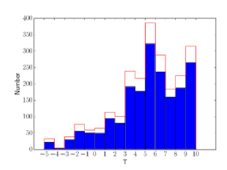
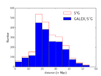
Figure 1.— Comparisons of the distributions of the $\mathrm{S^{4}G}$ sample (white bars) with the GALEX/$\mathrm{S^{4}G}$ subsample (filled bars). The distributions of numerical morphological types (T) (binning=1) (top-left), distances in Mpc (binning=5Mpc) (top-right), 3.6$\mu$m absolute AB magnitudes (binning=1mag) (bottom-left), and (FUV $-$ NUV) color (binning=0.25 mag) (bottom-right) of both samples are shown. The $\mathrm{S^{4}G}$ sample is comprised of 2352 galaxies, and the GALEX/$\mathrm{S^{4}G}$ subsample of 1931 galaxies. The 3.6$\mu$m absolute magnitude is accompanied by the logarithm of the stellar mass in the top x-axis, computed using eq.A6 in Appendix A. The vertical line at (FUV $-$ NUV) = 0.9 corresponds to the value used in Gil de Paz et al. (2007) to broadly separate between early and late-type galaxies.

2.2. GALEX counterparts

We gathered all available GALEX FUV and NUV images and related data products for 1931 $\mathrm{S^{4}G}$ galaxies that had been observed in at least one of these two UV bands. Over 200 galaxies do not have GALEX data at all. We obtained the original GALEX data using the GALEXview tool. Priority was given to galaxies that have both FUV and NUV images, with the longest FUV exposure time. If this condition was met for several product tiles (including a very similar exposure time to the NUV in the FUV), we chose the one where the target galaxy was best centered in the field-of-view (FOV). We collected imaging data from all kinds of surveys such as the All-sky Imaging Survey (AIS), Medium Imaging Survey (MIS), Deep Imaging Survey (DIS), Nearby Galaxy Survey (NGS), as well as from Guest Investigator (GIs/GIIs) Programs.

The collected data, once processed, yielded a total of 1931 galaxies with both FUV and NUV photometry available. We call this sample, derived from the $\mathrm{S^{4}G}$ and having FUV, NUV, as well as IRAC1 3.6 $\mu$m photometry, the GALEX/$\mathrm{S^{4}G}$ sample. We compare the $\mathrm{S^{4}G}$ sample and the GALEX/$\mathrm{S^{4}G}$ sample in Figure 1. The distributions of distances, apparent B-band magnitudes, and morphological types of the two samples and the distribution of the integrated (FUV $-$ NUV) colors of the final GALEX/$\mathrm{S^{4}G}$ sample are shown. Demographics are shown in Table 2. Our GALEX/$\mathrm{S^{4}G}$ sample is clearly representative of the whole $\mathrm{S^{4}G}$ sample with only minor differences in the case of the absolute magnitude distribution. Note that every $\mathrm{S^{4}G}$ galaxy targeteted with GALEX was detected and its UV fluxes measured.

We also subdivided the GALEX/$\mathrm{S^{4}G}$ sample into three other subsamples. This was done accordingly to the preliminary analysis of the UV-to-IR photometry of Bouquin et al. (2015), where we presented our sample of 1931 galaxies with their asymptotic magnitudes plotted on an (FUV $-$ NUV) vs (NUV $-$ [3.6]) color-color diagram. From this integrated color-color diagram, we were able to select three subsamples of galaxies, namely the GBS, the GRS, and the GGV galaxies, and were defined as follows:

GBS: $$0.12x+0.16-2\sigma_{\mathrm{GBS}}\leq y\leq 0.12x+0.16+2\sigma_{\mathrm{GBS}}$$ (1)

GRS: $$-0.23y+5.63-1\sigma_{\mathrm{GRS}}\leq x\leq-0.23y+5.63+1\sigma_{\mathrm{GRS}}$$ (2)

GGV: $$y>0.12x+0.16+2\sigma_{\mathrm{GBS}}\textrm{ and }x<-0.23y+5.63-1\sigma_{\mathrm{GRS}}$$ (3)

where $x$ = (NUV $-$ [3.6]), $y$ = (FUV $-$ NUV), $\sigma_{\mathrm{GBS}}$=0.20, and $\sigma_{\mathrm{GRS}}$=0.45. Both the GBS and GRS are defined to be stripes defined between two parallel lines (Equations 1 and 2). Note that the GRS equations are expressed in the $yx$-space. The GGV is the region bluer in (NUV $-$ [3.6]) than the GRS, but redder in (FUV $-$ NUV) than the GBS (Equation 3).

The GBS is populated by star-forming galaxies and mostly late-type galaxies while the GRS is populated by redder systems that lack star formation (quiescent) and are passively evolving or where only low levels of residual star formation are present (e.g., Boselli et al., 2005; Yıldız et al., 2017) and that are, morphologically speaking, mostly ETGs. The GGV galaxies are found between the GBS and the GRS in this UV-to-IR color-color plane, and they are special in the sense that these galaxies can be seen to have decreased star formation activity in recent epoch, hence their (FUV $-$ NUV) colors are redder than in GBS galaxies and their (NUV $-$ [3.6]) colors are bluer than in GRS galaxies. However, it should be noted that we do not exclude the possibility that this GGV populations could represent GRS galaxies that are being rejuvenated thus showing a blueing (FUV $-$ NUV) color. The important point here is that the quick response of the (FUV $-$ NUV) color to even small amounts of recent star formation, coupled to the tightness of the GBS, allows identifying galaxies that are just starting to experience these quenching or rejuvenating events. See Bouquin et al. (2015) for further details.

Table 2Galaxy sample demographics

Galaxy sample		N	Percentage relative to ()
$\mathrm{S^{4}G}$		2352	100%
GALEX/$\mathrm{S^{4}G}$		1931	82.1% ($\mathrm{S^{4}G}$)
GBS		1753	90.8% (GALEX/$\mathrm{S^{4}G}$)
GGV		70	3.6% —
GRS		79	4.1% —
Others		29	1.5% —
ETGs	E	24	1.2% (GALEX/$\mathrm{S^{4}G}$)
	E-S0	23	1.2% —
ETDGs	S0	51	2.6% —
	S0-a	103	5.3% —
	Sa	175	9.1% —
LTGs	Sb	340	17.6% —
	Sc	669	34.7% —
	Sd	168	8.7% —
	Sm	192	9.9% —
	Irr	186	9.6% —

3. ANALYSIS

In this section, we describe our method of analysis of the NIR and UV imaging data acquired by Spitzer IRAC1 and GALEX, in order to obtain 3.6 $\mu$m, FUV, and NUV surface photometry. The acquirement of the 3.6 $\mu$m surface photometry is not described here as it is already explained in Muñoz-Mateos et al. (2015), and we only focus on the FUV and NUV surface photometry in this article (Section 3.1). We also performed a radial normalization of the 3.6 $\mu$m radial profiles (Section 3.2). We also constructed the (FUV $-$ NUV), (FUV $-$ [3.6]), and (NUV $-$ [3.6]) color profiles (Section 3.3).

3.1. UV Surface photometry and asymptotic magnitudes

We obtained spatially resolved FUV and NUV surface photometry, as well as asymptotic magnitudes, for the 1931 galaxies in our GALEX/$\mathrm{S^{4}G}$ sample. Three types of GALEX data products were collected from the database:

• the intensity maps in FUV (*fd-int.fits) and NUV (*nd-int.fits),

• the high-resolution relative response maps in FUV (*fd-rrhr.fits) and NUV (*nd-rrhr.fits), and

• the object masks in both FUV (*fd-objmask.fits) and NUV (*nd-objmask.fits).

Once all data were gathered, we proceeded to reduce and analyze our GALEX UV sample in the same manner as in Gil de Paz et al. (2007).

First, a sky value was measured from the surroundings of the target galaxy. This was followed by the preparation of a mask, in two steps. In the first step of the masking process, we masked automatically unresolved sources that had (FUV $-$ NUV) colors redder than 1 mag, which masks out most foreground stars. This was followed by careful visual checks, verifying each and every single galaxy, and carefully editing the masks one by one, by manually adding or removing masks, since the automatization could: (a) falsely detect bulges, fail to select (b) companions, and (c) foreground blue stars, all for the benefit of preserving very blue star-forming regions, especially those in the outskirts of disk galaxies. We unmasked all affected bulges and tried to include as many star-forming regions falsely masked, while foreground stars were masked out as much as possible. In the process we also generated FUV+NUV RGB images for each galaxy that were used during the manual masking process in order to have an educated guess on any potential masking failure encountered. Although great care had been taken during this masking process, it should be noted that in some cases (e.g., merging galaxies, galaxies with bright stars nearby, objects at the edge of the FOV, bad image quality), difficult choices had to be made. We acknowledge that in those cases (less than a few percent) the values obtained may differ from those obtained by other authors (our masks can be provided on demand). Errors associated to these effects cannot be accounted for and are not included in Table 1.

Then, surface brightnesses were measured by averaging over annuli with the same position angle (PA) and ellipticity ($\epsilon$) as those used in the analysis of the $\mathrm{S^{4}G}$ sample IRAC data. We used a step in major-axis radius of 6$\arcsec$ and integrated over a width of $\pm$3$\arcsec$, also in major-axis radius. The total uncertainty in the surface brightness does take into account the contribution of both local and large-scale background errors (Gil de Paz et al., 2007).

In Figure 2, we show the FUV+NUV RGB postage stamp images. The resulting products, shown also in this figure, include the surface brightness radial profiles in both FUV and NUV in mag arcsec^-2, (FUV $-$ NUV) color profiles in mag arcsec^-2, and asymptotic magnitudes (in mag) for each galaxy. The obtained values are corrected for extinction due to the Milky Way. This foreground Galactic extinction was obtained following the UV extinction law of Cardelli et al. (1989), assuming a total to selective extinction ratio $R_{V}=A_{V}/E(B-V)=3.1$, giving the attenuation values of $A_{\mathrm{FUV}}=7.9E(B-V)$ and $A_{\mathrm{NUV}}=8.0E(B-V)$, where the reddening $E(B-V)$ from Galactic dust is obtained from the map of Schlegel et al. (1998). The surface photometry of the sample is not corrected for internal dust attenuation nor inclination of the host galaxy. A partial table including FUV and NUV surface photometry for 192 ETGs was first released by Zaritsky et al. (2015) and is also available in the VizieR online database (Ochsenbein et al., 2000).

In Table 3, examples of the values we obtained are shown. The graphical rendering of the data is shown in Figure 3 and is explained in the next subsection.

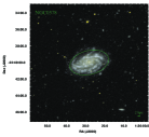
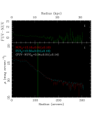
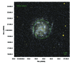
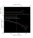
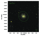
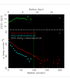
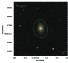
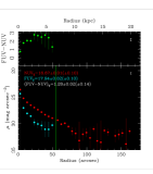
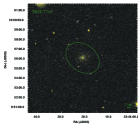
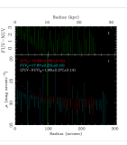
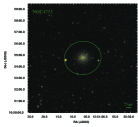
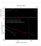
Figure 2.— GALEX RGB postage stamp images generated from FUV and NUV images (left) with their respective surface brightness $\mu_{FUV}$, $\mu_{NUV}$, and (FUV $-$ NUV) color profiles (right). The first row show typical Sc galaxies in the GBS, the second row show typical Sa galaxies in the GGV, and the third row show typical E galaxies in the GRS. The radial surface brightness profile (red dots for NUV, blue dots for FUV) as well as (FUV $-$ NUV) (in mag arcsec^-2) radial color profile (green dots), are shown. The green ellipse in the RGB image corresponds to the isophotal contour D25 at 25 mag arcsec^-2 in B-band. A 2 kiloparsec scale is shown in the bottom-right corner of the image.

3.2. IR profile radial normalization

Figure 3 shows the FUV, NUV and 3.6 $\mu$m surface brightness profiles $\mu_{\mathrm{FUV}}$, $\mu_{\mathrm{NUV}}$, and $\mu_{[3.6]}$ in units of mag arcsec^-2 plotted against the radius in kiloparsec in one case (left panels), and normalized in units of $R/R80$ in the other (right panels).

$R/R80$ is a distance unit that we devised based on the radius (i.e., semi-major axis of ellipse) that encloses 80% of the total 3.6 $\mu$m light and that we call $R80$. The innermost measurement is at 6$\arcsec$ semi-major axis radius, and the rest of the measurements radially outward in the disk are represented as small dots for each 6$\arcsec$ step. The very center is excluded because it could be affected by differences in the PSF amongst the three bands and by the contribution of an AGN. The SB measurements are taken up to 3 $\times$ D25, however, for the analysis, we select only measurements having errors less than 0.2 mag arcsec^-2. These errors include the total measurement uncertainties, dominated by Poisson noise in the centers and by sky uncertainties in the outskirts, but exclude any systematic zero-point uncertainty. Color-coding is based on the numerical morphological types and is the following: E is red, E-S0 is orange, S0 is yellow, S0-a is pink, Sa is light-green, Sb is dark-green, Sc is cyan, Sd is light-blue, Sm is dark-blue, and Irr is purple. Numerical morphological types were obtained from HyperLeda (Makarov et al., 2014) and follow the RC2 classification scheme: -5 $\leq$ E $\leq$ -3.5, -3.5 $<$ E-S0 $\leq$ -2.5, -2.5 $<$ S0 $\leq$ -1.5, -1.5 $<$ S0-a $\leq$ 0.5, 0.5 $<$ Sa $\leq$ 2.5, 2.5 $<$ Sb $\leq$ 4.5, 4.5 $<$ Sc $\leq$ 7.5, 7.5 $<$ Sd $\leq$ 8.5, 8.5 $<$ Sm $\leq$ 9.5, and 9.5 $<$ Irr $\leq$ 999. Galaxies with unknown morphological type are assigned the numerical type 999, and are included in the irregular galaxies (Irr) bin, as these are, in the vast majority of the cases, systems with ill-defined morphology.

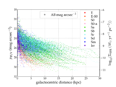
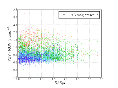
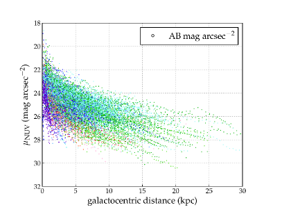
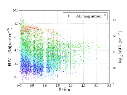
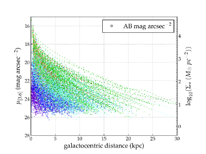
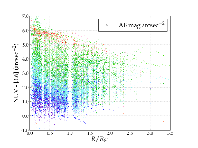
Figure 3.— Left column, top to bottom FUV, NUV, and [3.6] surface brightness versus radius in kiloparsec. Right column, top to bottom (FUV $-$ NUV), (FUV $-$ [3.6]), and (NUV $-$ [3.6]) colors vs $R/R80$. Each dot represents a data point. Our entire sample of 1931 galaxies is shown. Color-coding is based on the numerical morphological types and is the following: E is red, E-S0 is orange, S0 is yellow, S0-a is pink, Sa is light-green, Sb is dark-green, Sc is cyan, Sd is light-blue, Sm is dark-blue, and Irr is purple. The discretization seen in the right-hand plots is due to the fact that the $R80$ values derived from the analysis of our growth curves are obtained from the data point that encompasses a fraction of the light closest to 80% but it is not interpolated. The figures show that this translates in an error of no more than $\pm$0.1 $R/R80$.

3.3. Color profiles

The right column of Figure 3 shows each galaxy’s spatially resolved radial color profiles in (FUV $-$ NUV), (FUV $-$ [3.6]) and (NUV $-$ [3.6]) as a function of galactocentric distance both in kpc and $R/R80$ units. Each plot shows the corresponding color profile distribution for each galaxy, color-coded by morphological type. As mentioned above, measurements are taken every 6$\arcsec$ from the center of each galaxy, and each profile reaches the galactocentric distance where the error in either FUV, NUV or 3.6 $\mu$m surface brightness becomes 0.2 mag arcsec^-2 or larger, thus rejecting the data that follow. It should be noted that measurements are available up to 3 $\times$ D25, but are more dominated by sky uncertainties as we move radially outward.

Figure 4 shows the average surface brightnesses and colors per $R/R80$ bin of width 0.5, as well as the range of the scatter from the mean value in each bin, and per morphological type. It should be noted that the range appears to diminish as we move radially outward, but this is due to reaching the observation limits in each band.

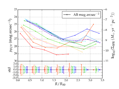
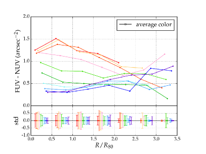
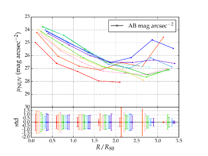
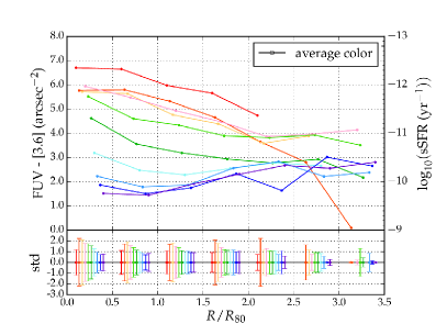
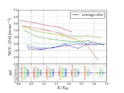
Figure 4.— Left column: top panel: Average surface brightness color-coded per morphological type per $R/R80$ bin of width 0.5. Bottom panel: the standard deviation (std) of the scatter from the mean, including the uncertainty, within each bin. A translation in x is applied for better visibility. It should be noted that the sample size substantially drops beyond $R/R80>1.5$ due to the observation limits in each band. Right column: The same but for color profiles.

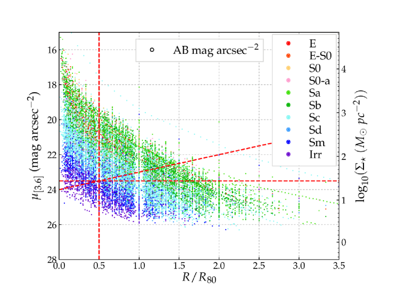
Figure 5.— 3.6 $\mu$m surface brightness profiles normalized to $R80$. The red dashed lines represent one example of the vertical and horizontal cutoffs, and another example of an oblique cutoff.

Table 3Surface brightness data (examples)

Name	r	$\mu_{FUV}$	$\mu_{NUV}$	$\mu_{[3.6]}$
	($\arcsec$)	mag/($\arcsec$)2	mag/($\arcsec$)2	mag/($\arcsec$)2
UGC00017	6	26.14$\pm$0.09	25.76$\pm$0.05	23.16$\pm$0.03
	12	26.32$\pm$0.10	25.86$\pm$0.05	23.60$\pm$0.05
	18	25.96$\pm$0.05	25.83$\pm$0.03	24.01$\pm$0.07
	24	26.47$\pm$0.05	26.23$\pm$0.03	24.49$\pm$0.11
	30	26.65$\pm$0.05	26.38$\pm$0.03	24.80$\pm$0.14
	36	26.91$\pm$0.06	26.63$\pm$0.03	24.99$\pm$0.17
	42	26.66$\pm$0.05	26.49$\pm$0.03	25.27$\pm$0.21
	…	…	…	…
ESO409-015	6	21.92$\pm$0.01	21.89$\pm$0.01	22.72$\pm$0.02
	12	23.39$\pm$0.02	23.23$\pm$0.01	23.50$\pm$0.04
	18	24.85$\pm$0.03	24.50$\pm$0.02	24.24$\pm$0.07
	24	25.95$\pm$0.05	25.52$\pm$0.03	24.98$\pm$0.14
	30	26.93$\pm$0.07	26.22$\pm$0.03	25.08$\pm$0.15
	36	27.63$\pm$0.09	26.87$\pm$0.05	25.62$\pm$0.24
	42	28.04$\pm$0.11	27.34$\pm$0.06	25.85$\pm$0.29
	…	…	…	…

4. RESULTS

The FUV and NUV are most sensitive to the presence and amount of (recently born) massive stars and, in particular, the FUV can be directly linked (modulo IMF) to the (observed) SFR, at least for late-type galaxies. In our preliminary work (Bouquin et al., 2015), we have seen that the majority of star-forming disk galaxies in our sample are distributed along the GBS, however, there exists some disk galaxies with redder, integrated, (FUV $-$ NUV) color that are located in the GGV. Spatially resolved color profiles allow us to see which parts of the galaxy are actually forming stars or not. Note that the (FUV $-$ NUV) color is quite reddening-free (but not extinction-free) for MW-like foreground dust and that even if that is not the case, the effect of dust in disks, especially in its outskirts, is smaller than that found between GBS and GRS galaxies (Muñoz-Mateos et al., 2007).

In order to study in more detail the disk component of a galaxy, we first need to isolate it by separating it from the bulge component. However, galaxies come in different shapes and sizes: some galaxies are bulgeless and only have a disk, whereas some others are diskless and only have a massive spheroidal component. We devised a method to isolate the disk component only from the 3.6 $\mu$m SB profiles, by applying a radial cutoff and a SB cutoff and finding the best linear fit to the outer parts of these NIR profiles (Section 4.1). This method allows us, regardless of the morphological type, to isolate the disk component and to obtain its scale-length and central surface brightness from the slope and y-intercept of the linear fit. With the spatially resolved photometry, we are able to construct a so-called star-forming main sequence, relating the FUV SB, $\mu_{\mathrm{FUV}}$, to SFR surface density and the 3.6 $\mu$m SB, $\mu_{[3.6]}$, to surface stellar mass density (Section 4.2). The sSFR can be directly obtained from the (FUV $-$ [3.6]) color (Section 4.3). We also explore the color-color diagrams obtained from these bands (Section 4.4). We show how the disks of GGV galaxies are also different from those of other galaxies (Section 4.5).

4.1. Disk separation using near-IR SB profiles.

Disks are known to have an exponential profile and are therefore close to a straight line in a surface brightness (a logarithm) versus galactocentric radius plot, at least in their inner regions. In the very outer regions, these single exponential profiles commonly bend (see Marino et al., 2016, and references therein). It should be noted in this context, however, that the level of either down- or up-bending in the surface brightness profiles of galaxy disks is usually minimized at near-infrared wavelengths (e.g. Muñoz-Mateos et al., 2011) (see also Bakos et al., 2008, for a comparison of these bending profiles at different wavelengths and in stellar mass).

In order to isolate the disk component in a coherent and reproducible way among all our 1884 disk galaxies (S0 and beyond) and to derive their multiwavelength properties, we have made use of the 3.6 $\mu$m surface brightness profiles of our sample and performed an error-weighted fit to our data points in $\mu_{[3.6]}$ versus galactocentric radius in kpc. Prior to this fitting, the surface brightnesses were corrected for geometrical inclination effects by adding $-2.5\log_{10}(b/a)$ (mag arcsec^-2), where $a$ and $b$ are the semi-major and semi-minor axes in the B-band, to each data point. No internal dust attenuation correction is applied. This has the effect of dimming the surface brightness for inclined systems (Graham & Worley, 2008). See Section 5 on how this inclination correction affects the comparison with the models. Then, we identified the position beyond which the profile starts to be best described by an exponential law at these wavelengths. In order to exclude the bulge (i.e. either the region where the Sérsic index is significantly larger than unity or the steepening associated to a pseudo-bulge) and given that we have in hand $R80$ measurements (major-axis radius where 80% of the IR light is enclosed) for the entire sample we remove the inner part of the profile up to some factor of $R80$ to perform different sets of fits. For this analysis we explored $R/R80$ cutoff factors of 0, 0.25, 0.50, 0.75, 1.00, and 1.25 and evaluated how far we should go from the galaxy center in each case to have good linear fits as given by the corresponding sample-averaged reduced $\chi^{2}$ values (see below). We combined this inner cutoff in $R/R80$ with cutoffs in surface brightness magnitude in the range $\mu_{[3.6]}$=21.5 $\sim$ 24 mag arcsec^-2, so only points fainter than the corresponding cutoff would be considered for the fit.

The rationale for using a combination of the two parameters is that we should normalize to the size of the objects to (1) do a first-order separation between bulges and disks and (2) take into account the fact that early-type systems usually have large, massive bulges with brighter near-infrared surface brightnesses than the disks of late-type spirals. Thus, when we cut in surface brightness we exclude larger regions in massive early-type systems and only the very central regions of very late-type spirals (see Figure 3, bottom-right plot). However, we should certainly add a quality-of-fit criterion here to determine the goodness of these criteria.

In order to determine the reduced-$\chi^{2}$ for each fit, the number of degrees-of-freedom (d.o.f.) is computed as the number of data points that remain after applying the corresponding cutoffs minus the number $P$ of free parameters, where $P=2$ in our linear fitting case (see Andrae et al., 2010, for a discussion). Average reduced-$\chi^{2}$ are computed for each combination of cutoffs and the results are shown in Table 4.

Table 4Average reduced-$\chi^{2}$ of the linear-fit with $\mu_{[3.6]}$ and $R/R80$ cuts

		$R/R80$ cutoffs
		0.00		0.25		0.50		0.75		1.00		1.25
		$<\chi^{2}>$	N	$<\chi^{2}>$	N	$<\chi^{2}>$	N	$<\chi^{2}>$	N	$<\chi^{2}>$	N	$<\chi^{2}>$	N
$\mu_{[3.6]}$ cutoffs	21.5	26.20	(1577)	20.84	(1554)	15.72	(1451)	9.68	(1240)	4.04	(794)	2.87	(535)
	22	10.64	(1489)	8.63	(1474)	6.97	(1387)	5.85	(1191)	3.26	(781)	2.48	(530)
	22.5	4.89	(1384)	4.28	(1375)	3.54	(1298)	3.11	(1126)	2.02	(756)	1.62	(518)
	23	2.34	(1232)	2.17	(1228)	1.81	(1165)	1.63	(1014)	1.14	(693)	0.98	(482)
	23.5	1.37	(1034)	1.28	(1033)	gray!251.12	gray!25 (987)	0.96	(863)	0.68	(591)	0.56	(419)
	24	0.78	(755)	0.77	(754)	0.73	(723)	0.67	(630)	0.40	(426)	0.35	(296)

Table 5Average reduced-$\chi^{2}$ of the linear-fit in the $\mu_{[3.6]}$ vs $R/R80$ plane with oblique cuts

		slope (a) cutoff
		-6		-5		-4		-3		-2		-1
		$<\chi^{2}>$	N	$<\chi^{2}>$	N	$<\chi^{2}>$	N	$<\chi^{2}>$	N	$<\chi^{2}>$	N	$<\chi^{2}>$	N
y-intercept (b) cutoff	20	777.55	(1717)	649.14	(1716)	569.63	(1713)	469.68	(1712)	393.01	(1707)	304.54	(1699)
	22	205.61	(1697)	158.46	(1691)	129.09	(1684)	88.95	(1668)	52.78	(1644)	27.10	(1592)
	24	61.96	(1633)	44.50	(1607)	28.48	(1563)	13.20	(1528)	5.58	(1412)	gray!252.07	gray!25(1233)
	25	33.19	(1578)	23.64	(1540)	11.19	(1482)	6.19	(1375)	2.21	(1202)	0.78	(831)
	26	20.87	(1516)	10.53	(1445)	6.24	(1339)	2.50	(1166)	0.96	(845)	0.44	(219)
	28	6.20	(1260)	3.12	(1090)	1.74	(838)	0.89	(471)	0.79	(127)	0.72	(5)
	30	2.46	(858)	1.56	(596)	0.87	(322)	1.27	(103)	1.04	(8)	$\cdots$	(0)

When doing these fits we excluded elliptical galaxies ($T$ $\leq$ $-$3.5) in all cases. It should be noted that as we move towards higher values in both the $R/R80$ and $\mu_{[3.6]}$ cutoffs, the number of points used for the linear fit decreases, and the number of galaxies that can be analyzed becomes smaller. This is because some galaxy profiles do not reach beyond the cutoffs, or only one data point is beyond them. Besides, eventually the reduced-$\chi^{2}$ goes below unity, telling us that we are overfitting the data. This is in part due to the effect of correlated errors associated to the uncertainties in the sky subtraction in the very outer surface brightness measurements. We find that the best set of $R/R80$ and $\mu_{[3.6]}$ cutoffs, i.e., the one that yields an average reduced-$\chi^{2}\sim 1$ with still a large number of galaxies, is at $R/R80$=0.5 and $\mu_{[3.6]}$=23.5 mag arcsec^-2, where $<$$\chi^{2}$$>$=1.12 and the number of galaxies is 987 ($\sim$51% of the GALEX/$\mathrm{S^{4}G}$ sample; see Figure 5).

We also apply oblique cuts in the $\mu_{[3.6]}$ versus $R/R80$ plane instead of a combination of vertical and horizontal cuts. Table 5 shows the resulting average reduced-$\chi^{2}$ and the number of galaxies for a combination of cutoff slopes $a$ and cutoff $y$-intercepts $b$. We tried all the combinations of slopes ranging from $-$7 to $-$1 (in units of mag arcsec^-2/($R/R80$)) and $y$-intercepts between 20 and 30 mag arcsec^-2. The best compromise between average reduced-$\chi^{2}$ and number of galaxies is for slope and y-intercept values of $a$=$-$1 and $b$=24 mag arcsec^-2 where the average reduced-$\chi^{2}=2.07$ and the number of galaxies is 1233 ($\sim$64% of the GALEX/$\mathrm{S^{4}G}$ sample; see Figure 5). Graphical representations of the slopes and $y$-intercepts at these best cutoffs are shown in Figure 6.

The relatively good isolation of the disk component by some of these sets of criteria opens the door to statistical studies of the photometric properties of disks in thousands or millions of galaxies using existing data (SDSS) or data from future facilities and missions such as LSST or EUCLID.

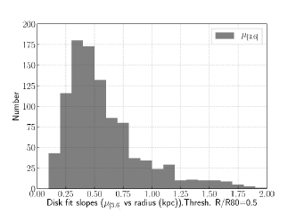
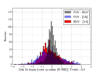
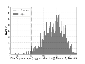
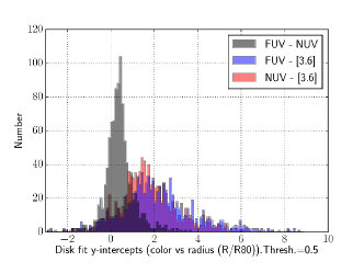
Figure 6.— Distributions of the best-fitting coefficients to the surface brightness and color profiles of disks. The fitting is performed beyond a radius $R/R80$=0.5 using points where the surface brightness is fainter than $\mu_{[3.6]}$=23.5 mag arcsec^-2. Top left: the distribution of slopes obtained in the $\mu_{[3.6]}$ vs kpc plane. Bottom left: the distribution of $y$-intercepts obtained in that plane. These correspond to the central surface brightness contribution of the disks. The dashed vertical line corresponds to the Freeman (1970) value, or the B-band central surface brightness for spirals $<\Sigma_{0}>$=21.48 B-mag arcsec^-2, converted to a 3.6 $\mu$m value of 18.2 mag arcsec^-2, assuming an average central color of (B_Vega $-$ [3.6]_AB) = 3.32 mag. Top right: the distribution of slopes obtained in the (FUV $-$ NUV), (FUV $-$ [3.6]), and (NUV $-$ [3.6]) vs $R/R80$ planes, i.e. the color gradients. Bottom right: the distribution of $y$-intercepts obtained in those planes, or, central colors of the disks. Bin width is 0.1 in all cases [in units of either mag or mag/($R/R80$)].

4.2. Spatially resolved star-forming main sequence from UV and near-IR SB profiles

In Figure 7 we plot the FUV surface brightness $\mu_{FUV}$ versus the 3.6 $\mu$m surface brightness $\mu_{[3.6]}$ for galaxies belonging to the GBS, GGV, and GRS subsamples based on their integrated colors. Both axes are expressed in mag arcsec^-2.

This figure can be also seen as a comparison between the observed SFR (i.e. not-corrected for internal dust extinction) and the stellar mass surface densities (see Appendix A), except for those cases where the FUV emission is not due to young massive stars. In that regard, this point is equivalent to the star formation main sequence (SFMS) but in surface brightness (see Cano-Díaz et al., 2016).

Each data point is the averaged value within fixed-inclination elliptical ring apertures of 6$\arcsec$ width. The innermost ring has a semi-major axis length of 6$\arcsec$ with a width of 6$\arcsec$, defined by an inner ellipse with a major axis of 3$\arcsec$ from the center and an outer ellipse with a semi-major axis of 9$\arcsec$ from the center. The initial ring does not cover the center of the galaxy as this could be affected by differences in the PSF amongst the three bands and by the contribution of an AGN. Subsequent rings increase in size in 6$\arcsec$ steps, i.e., they have semi-major axis radii of 12$\arcsec$, 18$\arcsec$, 24$\arcsec$, and so on.

For early-type GRS galaxies, the FUV and 3.6 $\mu$m surface brightnesses show a pretty tight correlation, which indicates that the 3.6 $\mu$m emission traces not only the stellar mass, but also the bulk of the stars dominating the FUV emission in these objects, mainly main-sequence turn-off or extreme horizontal branch (EHB) stars, depending on the strength of the UV-upturn. Despite the large scatter of the GRS found in Bouquin et al. (2015), the use of spatially resolved data with the 3.6 $\mu$m surface brightness as normalizing parameter leads now to a very tight GRS in this SB-SB plane (or a very small range in FUV $-$ [3.6] color). The comparison of these profiles with those of the GGV galaxies shows that in the latter case the central stellar mass surface density is 1.5-2 mag fainter than in the former and that most GGV galaxies (all except the few very late-type GGVs) have (outer) disks that follow a trend similar to that followed by the outer regions of GRS galaxies. Finally, late-type galaxies in the GBS span a large range of values in both $\mu_{FUV}$ and $\mu_{[3.6]}$. Irregulars, Sm, and Sd galaxies have the highest SFR surface densities (for a given stellar mass surface density) amongst the GBS subsample.

Despite the large scatter of GBS galaxies, they can be clearly distinguished from the early-type galaxies of the GRS and even GGV galaxies by looking at the (observed) sSFR values in their disks. Thus, while GBS disks have sSFR values that are higher than 10^-11.5 yr^-1, the outer regions of GGV and GRS galaxies are in the majority of the cases (all in the case of the GRS) below this value. This value could be used to easily discriminate between star-forming and quiescent regions within galaxies.

GBS galaxies define a well separated sequence, and with the spatial information now available, we can now see what parts of the galaxies are now just leaving the GBS, that is, have their SF suppressed or exhausted. While a few GGV galaxies show a decrease in the sSFR of their inner regions, most of these galaxies are within the locus of the GBS in the inner parts but approach the sequence marked by the GRS profiles in their outer regions. In other words, the fact that these galaxies where identified as leaving the GBS in Bouquin et al. (2015) is mainly due to their outer parts, likely caused by the disks of GGV galaxies undergoing either an outside-in SF quenching or an inside-out rebirth.

It is worth emphasizing here that only the combined use of FUV, NUV, and 3.6 $\mu$m allows properly separating the ”classical blue cloud” (now blue sequence) and the ”classical red sequence” and determining which galaxies are now leaving (or entering) the GBS and what regions within galaxies are responsible for it.

We mark in Figure 7 the $\mu_{[3.6]}$ value that corresponds to the surface stellar mass density of $\Sigma_{\star}=3\times 10^{8}$ $M_{\odot}$ kpc^-2 = 300 $M_{\odot}$ pc^-2 ($\mu_{[3.6]}=20.89$ mag arcsec^-2) proposed by Kauffmann et al. (2006) to separate between bulge-dominated and disk-dominated objects.

In the case of our GBS galaxies, this stellar mass surface density indicates the region inside which the SFR surface density flattens relative to the stellar mass surface density, i.e. when the (FUV $-$ [3.6]) color becomes significantly redder (see Figure 9). A similar change is observed when using light-weighted age of the stellar population in galaxies instead (González Delgado et al., 2014).

The sSFR of the outer parts (beyond $\mu_{[3.6]}$ = 20.89 mag arcsec^-2) is shown in Figure 8 for GBS, GGV, and GRS galaxies. This is done simply by calculating the linear scale sSFR of one galaxy, at each point that are in the outer parts, and averaging these sSFR values (not light/mass weighted) in order to get a single sSFR value per galaxy (and expressing them in the logarithmic scale at the end). We find the following specific star formation rate density range: $-$12.5 $<$ $\log_{10}(\mathrm{sSFR})$ $<$ $-$9.5 for GBS galaxies, $-$12.4 $<$ $\log_{10}(\mathrm{sSFR})$ $<$ $-$9.8 for GGV galaxies, and $-$12.6 $<$ $\log_{10}(\mathrm{sSFR})$ $<$ $-$11.7 for GRS galaxies. Since we do not correct for internal dust attenuation, these values should be viewed as lower limits of the true sSFR. Previous studies of the impact of dust on the (FUV $-$ [3.6]) colors (Muñoz-Mateos et al., 2007, 2009a, 2009b) have shown that dust attenuation A_FUV decreases as we move outward in the disks, although the dust content differs from one morphological type bin to another, for example, Sb-Sbc galaxies have higher A_FUV at all radii than the other types, whereas Sdm-Irr have relatively very low dust content. It should be noted, however, that besides dust, the reddening in the outer parts of quiescent galaxies is due to their older stars. There is a clear difference between the outer parts of GRS galaxies having low sSFR and a narrow range of values, and those of GBS galaxies with a wide range of sSFR but in general not as low as the outer parts of the GRS. For our sample, we have a distribution in outer disks sSFR with the mean at $-$10.6 dex and $\sigma$=0.5 dex (rms) for GBS, $-$11.5 dex and $\sigma$=0.7 dex for GGV, and $-$12.3 dex and $\sigma$=0.2 dex for GRS galaxies. The sSFR of the outer parts of GGV galaxies in our sample covers a wider range of values but is not as high as some GBS galaxies, and not as low as some GRS galaxies. Note that in the case of the GRS galaxies, the UV emission might not be due to recent SF but to the light from low-mass evolved stars.

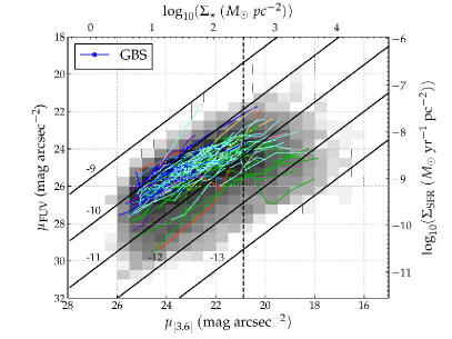
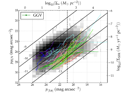
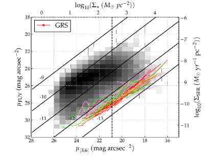
Figure 7.— FUV surface brightness versus 3.6 $\mu$m surface brightness for randomly selected GBS (top), all the GGV (middle) and all the GRS galaxies (bottom) subsamples. The diagonal solid lines represent constant sSFR, and are annotated with the decimal exponent of the logarithm. These plots are equivalent to the (observed) Star Formation Main Sequence (SFMS) but in surface brightness. Both the segregation in sSFR between the GBS, GGV and GRS and the bending at high (surface density) masses toward lower sSFR values are also clear in this plot. The vertical black dashed line corresponds to $\Sigma_{\star}$ = $3\times 10^{8}$ $M_{\odot}$ $kpc^{-2}$ (or $\mu_{[3.6]}=20.89$ mag arcsec^-2) (Kauffmann et al., 2006). The 2D density histogram shown in the background of each panel represents the data points density of GBS galaxies.

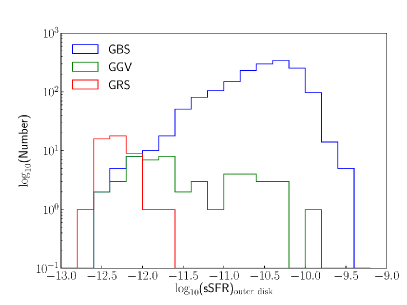
Figure 8.— Decimal log-log histogram of the mean sSFR obtained by fitting the outer disk part (beyond $\mu_{[3.6]}=20.89$ mag arcsec^-2) of GBS, GGV, and GRS galaxies. The bin size is 0.2 dex.

4.3. Color and sSFR profiles

Figure 9 shows the GRS (top row), GGV (center row), GBS (bottom row) galaxies’ (FUV $-$ [3.6]) color profiles versus 3.6 $\mu$m surface brighntess $\mu_{[3.6]}$, with the same color-coding per morphological type as in previous plots. Again, the 3.6 $\mu$m surface brightness corresponds to the stellar mass per area (see eq. A8 in Appendix A), and the (FUV $-$ [3.6]) color is equivalent to the observed (not corrected for internal extinction) sSFR (units $yr^{-1}$) (see eq. B6 in Appendix B).

The yellow star symbol corresponds to the radial measurement where the cumulative magnitude at 3.6 $\mu$m reaches 80% of the enclosed light at these wavelength.

The (FUV $-$ [3.6]) color profiles are very different for the GRS, GGV, and GBS subsamples. In the case of GRS galaxies, which are mostly early-type but not exclusively, the color is tightly constrained within a range from 6 to 8 mag but gets a bit bluer to the outer regions, especially for GRS galaxies of S0, Sa, Sb, and Sc morphological types.

On the other hand, in the case of GBS galaxies, their (FUV $-$ [3.6]) color ranges from $-$1 to 10 mag, corresponding to a sSFR value ranging from $10^{-10}$ to $10^{-13}$ yr^-1. Regarding the differences in the color profiles for each galaxy type, Sa, Sb, and Sc galaxies go from red to blue inside-out, while Sd, Sm, and Irregulars are much bluer than Sa, Sb, and Sc at a given stellar mass surface density but their color gradients are somewhat flatter. Again, it should be noted that we are not correcting for dust and that the effect of dust is to redden the (FUV $-$ [3.6]) color (Muñoz-Mateos et al., 2007) and therefore yields a lower limit to the sSFR.

The fact that most profiles of GBS galaxies become bluer from inside-out indicates that the lower the surface stellar mass density (the greater the galactocentric distance) the greater the sSFR, i.e., the higher the SFR for a given surface stellar mass density, the more stars are born in the outskirts. Correcting for internal dust extinction, assuming that dust extinction and reddening effects are stronger in the inner regions than the outer parts, would yield bluer centers compared to the outer disk. This has the effect of increasing the slope of the gradient, where negative color gradients would become flatter, and positive color gradients even more positive. Such effect would translate to a less-pronounced degree of inside-out growth. It should be noted that while the internal dust-correction would affect the color profiles of the galaxies, it is not enough to explain why most galaxies are becoming bluer inside-out (see Figure 2 in Muñoz-Mateos et al., 2007). Studies by Muñoz-Mateos et al. (2007, 2011); Pezzulli et al. (2015) on nearby galaxy samples have shown that mass growth and radial growth of nearby spiral disks, growing inside-out, have timescales on the order of $\sim$10 Gyr and  30 Gyr, respectively. Isolating a few galaxies actively forming stars in their outer regions, reveals that their outer regions fall indeed near $\log_{10}$(sSFR) $\sim$ $-$10 yr^-1, or $\sim$10 Gyr, in agreement with the above work (see GBS plot in Figure 9). In the case of profiles reddening in the outskirts, the lower $\Sigma_{\star}$ becomes, the smaller the sSFR.

Remarkably, a clear color flattening is observed in the outer parts of the profiles of most GBS galaxies when $\Sigma_{\star}$$<$ 300 $M_{\odot}$ pc^-2. Applying a weighted linear fit to the left-hand-side and right-hand-side of $\mu_{[3.6]}=20.89$ mag arcsec^-2, we get $(\mathrm{FUV}-[3.6])=(-0.395\pm 0.023)\cdot\mu_{[3.6]}+(11.537\pm 0.453)$, and $(-0.438\pm 0.009)\cdot\mu_{[3.6]}+(12.210\pm 0.193)$ respectively. These are shown in Figure 9 as solid blue lines for the mean value, accompanied by parallel dashed blue lines corresponding to the 1$\sigma$ uncertainty.

The galaxies falling into the GGV category globally are clearly distinct from the GBS ones also in terms of their spatially resolved properties. They show flat or even inverted color (and sSFR) profiles as a function of stellar mass surface density (hardly due to radial variations in the amount of dust reddening; see Muñoz-Mateos et al., 2007), which indicates either a decline in the observed SFR (oblique lines in Figure 9) in their outskirts or, alternatively, a recent enhancement of the SFR in the inner regions of an otherwise passively evolving system. In the latter case, the low fraction of intermediate-type spirals in the GRS (compared to the GGV) suggests that this rebirth should be accompanied by a morphological transformation from ETGs towards later galaxy types. There are, indeed, post-starburst (E+A) or (K+A) galaxies that are in the classical green valley (French et al., 2015) that did have centrally concentrated star formation (Norton et al., 2001).

In the more likely case of a decline of the SFR in the outer disks of GGV intermediate-type-spirals we should then invoke the presence of a quenching (or, at least, damping) mechanism for the star formation acting primarily in these regions.

Figure 10 shows the color profiles of (FUV $-$ NUV), (FUV $-$ [3.6]), and (NUV $-$ [3.6]) vs $\mu_{[3.6]}$ surface brightness. Linear fits to these color profiles were performed for each individual galaxy and are included in Table 7. The fits were performed for SB fainter than $\mu_{[}3.6]$ = 20.89 mag arcsec^-2 in these cases.

While a positive gradient seems to be more pronounced in (FUV $-$ NUV) color compared to the other two, it is not clear what is driving it. Since dust reddening is rarely increasing toward the outer parts, those objects with positive (FUV $-$ NUV) color gradients are likely suffering changes in the recent SF history of their outer regions. The dominant morphological type of positive (FUV $-$ NUV) color gradient galaxies are S0-a galaxies.

The comparison between the (NUV $-$ [3.6]) and (FUV $-$ [3.6]) color profiles (both shown in Figure 10) is also important to determine whether the UV emission is coming from newly formed O and B stars, or from evolved UV-upturn sources (likely associated to extreme horizontal branch stars; see also Section 4.4, which mainly contribute to the FUV band; O’Connell, 1999).

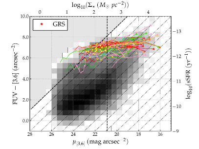
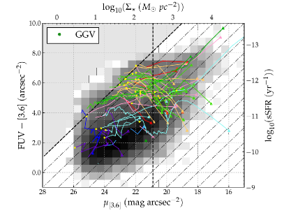
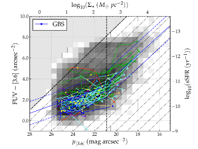
Figure 9.— (FUV $-$ [3.6]) color versus $\mu_{[3.6]}$ surface brightness for the radial profiles of GRS top row, GGV middle row, and GBS bottom row galaxies. Each galaxy’s center (within 6$\arcsec$ of the central most aperture) is represented by a triangle, and subsequent values are taken at every 6$\arcsec$ and are represented by smaller dots if these values exist. Values (dots) belonging to the same galaxy are connected by a line of the same color as the dots. The yellow star shows the radial distance at which 80% of the 3.6 $\mu$m light is enclosed. Diagonal dot-dashed lines are lines of constant $\mu_{\mathrm{FUV}}$ arcsec^-2 (i.e. observed SFR surface density), with the left-most dashed line corresponding to $\mu_{\mathrm{FUV}}$ = 29 ABmag arcsec^-2 (corresponding to $\Sigma_{\mathrm{SFR}}=4.36\times 10^{-5}$ $M_{\odot}/yr/kpc^{2}$ for a Kroupa IMF), the approximate sensitivity limit of our GALEX observations. The vertical black dashed line corresponds to $\Sigma_{\star}$ = $3\times 10^{8}$ $M_{\odot}$ $pc^{-2}$ (or $\mu_{[3.6]}=20.89$ mag arcsec^-2) (Kauffmann et al., 2006). The solid blue lines that go through the data points in the GBS plot are the fits to all the data points on each side of $\mu_{[3.6]}=20.89$. The parallel dashed blue lines show the $\pm 1\sigma$ (rms) of the distribution. In the case of the GBS plot, we show randomly-selected galaxies to better illustrate how GBS galaxies behave. In all cases, the entirety of the data is shown as a logarithmic 2D density histogram with 0.5 $\times$ 0.5 binning, where darker (brighter) shades mean higher (lower) data point density.

Table 6COLOR AND SURFACE BRIGHTNESS GRADIENTS FROM RADIAL PROFILES NORMALIZED TO $R80$ (except for $\mu_{[3.6]}$)

	FUV $-$ NUV		FUV $-$ [3.6]		NUV $-$ [3.6]		$\mu_{[3.6]}$
unit	mag/($R/R80$)		mag/($R/R80$)		mag/($R/R80$)		mag/kpc
name	a	b	a	b	a	b	a	b
ESO293-034	-0.03$\pm$0.06	0.48$\pm$0.07	-1.31$\pm$0.12	4.30$\pm$0.13	-1.37$\pm$0.09	3.91$\pm$0.09	0.55$\pm$0.02	21.41$\pm$0.14
NGC0007	0.15$\pm$0.42	0.21$\pm$0.34	-0.11$\pm$0.48	1.64$\pm$0.39	-0.25$\pm$0.14	1.42$\pm$0.11	—$\pm$—	—$\pm$—
IC1532	-0.76$\pm$0.92	0.96$\pm$0.66	-0.12$\pm$0.95	2.44$\pm$0.67	0.63$\pm$0.01	1.48$\pm$0.01	—$\pm$—	—$\pm$—
NGC0024	0.00$\pm$0.02	0.34$\pm$0.02	-0.54$\pm$0.05	3.04$\pm$0.04	-0.58$\pm$0.05	2.74$\pm$0.04	1.04$\pm$0.03	20.81$\pm$0.12
ESO293-045	0.05$\pm$0.07	0.08$\pm$0.06	-0.83$\pm$0.41	1.20$\pm$0.33	-0.92$\pm$0.36	1.15$\pm$0.29	0.64$\pm$0.03	23.15$\pm$0.12
UGC00122	1.01$\pm$0.21	-0.63$\pm$0.16	1.16$\pm$0.30	-0.23$\pm$0.23	0.15$\pm$0.25	0.40$\pm$0.19	0.81$\pm$0.04	24.24$\pm$0.10
NGC0059	0.09$\pm$0.11	1.60$\pm$0.09	0.18$\pm$0.11	4.82$\pm$0.09	0.10$\pm$0.05	3.21$\pm$0.04	2.23$\pm$0.07	21.38$\pm$0.09
ESO539-007	-1.11$\pm$1.14	0.97$\pm$0.90	-5.36$\pm$0.44	4.58$\pm$0.33	-3.73$\pm$0.71	3.22$\pm$0.50	0.24$\pm$0.04	24.37$\pm$0.14
ESO150-005	-0.27$\pm$0.18	0.36$\pm$0.14	-0.77$\pm$0.50	1.89$\pm$0.35	-0.56$\pm$0.40	1.57$\pm$0.28	0.24$\pm$0.04	24.19$\pm$0.14
NGC0100	0.87$\pm$0.18	0.02$\pm$0.12	-1.15$\pm$0.85	4.10$\pm$0.57	-2.05$\pm$0.68	4.10$\pm$0.45	—$\pm$—	—$\pm$—
NGC0115	0.06$\pm$0.04	0.16$\pm$0.04	-0.48$\pm$0.13	1.83$\pm$0.11	-0.51$\pm$0.13	1.63$\pm$0.11	0.52$\pm$0.03	21.27$\pm$0.17
UGC00260	0.04$\pm$0.07	0.29$\pm$0.09	-1.29$\pm$0.13	3.76$\pm$0.16	-1.43$\pm$0.14	3.57$\pm$0.16	0.27$\pm$0.02	22.96$\pm$0.26
NGC0131	0.11$\pm$0.08	0.34$\pm$0.08	0.00$\pm$0.12	2.86$\pm$0.10	-0.15$\pm$0.08	2.55$\pm$0.06	—$\pm$—	—$\pm$—
UGC00320	0.12$\pm$0.17	0.20$\pm$0.15	0.15$\pm$0.46	1.61$\pm$0.36	-0.01$\pm$0.31	1.44$\pm$0.23	0.50$\pm$0.03	22.88$\pm$0.17
…
Total	1541		1541		1541		992

• Same nomenclature as the $\mathrm{S^{4}G}$.

• Slope of linear fit and 1-$\sigma$ uncertainty obtained with scipy.optimize.curve package. We applied the cutoffs at $R/R80$=0.5 and $\mu_{[3.6]}$=23.5 mag arcsec^-2 only to the linear fit to the $\mu_{[3.6]}$ vs kpc data. In the case of colors, only the radial cutoff at $R/R80$=0.5 is applied. We also applied a simple inclination correction to the data by adding $-2.5\log_{10}(b/a)$ where $a$ and $b$ are the semi-major and semi-minor axes respectively.

• Y-intercept of linear fit with uncertainty.

• Total number of successful fits for each column. There are three galaxies with $T<-3.5$ (E galaxies, namely ESO548-023, NGC4278, and NGC5173) that are included in the $\mu_{[3.6]}$ vs kpc column, bringing the total to 992 galaxies, but are removed from the subsample for further analysis.

Table 7GRADIENTS OF COLOR VERSUS 3.6 MICRON SURFACE BRIGHTNESS PROFILES

	(FUV $-$ NUV)/$\mu_{[3.6]}$		(FUV $-$ [3.6])/$\mu_{[3.6]}$		(NUV $-$ [3.6])/$\mu_{[3.6]}$
unit	mag/(mag/arcsec2)		mag/(mag/arcsec2)		mag/(mag/arcsec2)
name	a	b	a	b	a	b
UGC00017	-0.03$\pm$0.08	0.94$\pm$1.92	-0.69$\pm$0.18	18.83$\pm$4.39	-0.63$\pm$0.10	17.21$\pm$2.30
ESO409-015	0.21$\pm$0.03	-4.78$\pm$0.64	0.93$\pm$0.07	-21.89$\pm$1.64	0.72$\pm$0.05	-17.13$\pm$1.08
ESO293-034	-0.01$\pm$0.02	0.79$\pm$0.48	-0.40$\pm$0.04	11.81$\pm$0.88	-0.42$\pm$0.03	11.61$\pm$0.62
NGC0210	-0.09$\pm$0.04	2.27$\pm$0.96	-1.01$\pm$0.18	26.28$\pm$4.03	-0.79$\pm$0.13	20.81$\pm$2.84
ESO079-005	-0.04$\pm$0.03	1.33$\pm$0.75	-0.40$\pm$0.10	10.96$\pm$2.41	-0.40$\pm$0.08	10.69$\pm$1.76
NGC0216	0.26$\pm$0.01	-5.20$\pm$0.22	0.39$\pm$0.03	-5.96$\pm$0.74	0.13$\pm$0.03	-0.74$\pm$0.60
PGC002492	-0.09$\pm$0.03	2.30$\pm$0.64	-0.50$\pm$0.05	13.43$\pm$1.23	-0.46$\pm$0.05	12.20$\pm$1.18
IC1574	0.19$\pm$0.05	-4.10$\pm$1.20	0.64$\pm$0.16	-13.28$\pm$3.86	0.41$\pm$0.13	-8.35$\pm$2.98
NGC0244	0.24$\pm$0.09	-4.96$\pm$1.99	0.38$\pm$0.03	-6.72$\pm$0.75	0.13$\pm$0.06	-1.45$\pm$1.32
PGC002689	-0.08$\pm$0.05	1.99$\pm$1.13	-0.08$\pm$0.19	2.80$\pm$4.53	0.03$\pm$0.16	0.11$\pm$3.78
UGC00477	-0.04$\pm$0.05	1.17$\pm$1.21	-0.68$\pm$0.06	17.59$\pm$1.43	-0.63$\pm$0.03	16.10$\pm$0.71
ESO411-013	-0.25$\pm$0.15	6.24$\pm$3.58	-0.50$\pm$0.07	13.91$\pm$1.60	-0.35$\pm$0.19	10.11$\pm$4.56
NGC0247	-0.06$\pm$0.02	1.76$\pm$0.51	-0.23$\pm$0.11	7.87$\pm$2.33	-0.10$\pm$0.09	4.73$\pm$1.95
…
Total	1650		1650		1650

• Same nomenclature as the $\mathrm{S^{4}G}$. Sorted by right ascension.

• Slope of linear fit and 1-$\sigma$ uncertainty obtained with scipy.optimize.curve package. We applied the cutoff $\mu_{[3.6]}$=20.89 mag arcsec^-2. No inclination correction is applied in these cases.

• Y-intercept of linear fit with uncertainty.

• Total number of successful fits for each column.

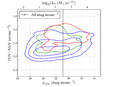
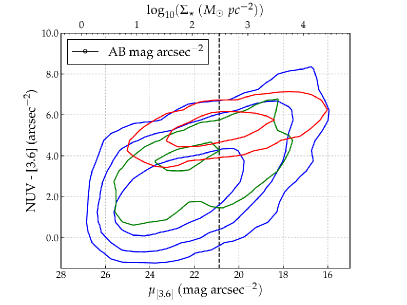
Figure 10.— (FUV $-$ NUV), (FUV $-$ [3.6]) and (NUV $-$ [3.6]) colors vs $\mu_{[3.6]}$ surface brightness profiles contours for GBS, GGV, and GRS galaxies. Contours levels were slightly smoothed with a gaussian kernel and describe the number density of SB profiles data points. The outer most level corresponds to number densities of 0 dex (i.e. at least one data point) in each 2D bins (the binning is 0.1 mag for (FUV $-$ NUV) color, and 0.5 mag for everything else). Then each contour level corresponds to an increase in number density by 1 dex. In the case of the (FUV $-$ [3.6]) vs $\mu_{[3.6]}$ diagram, diagonal lines represent constant FUV surface brightness $\mu_{FUV}$, with the right-most dashed line corresponding to $\mu_{FUV}$ = 29 ABmag arcsec^-2 (at the grey boundary), and decreasing by unity for each diagonal to the left. These are equivalent to lines of constant observed SFR surface density. The vertical black dashed line corresponds to $\log_{10}$($\Sigma_{\star}$ ($M_{\odot}$ $pc^{-2}$))=2.477 (or $\mu_{[3.6]}=20.89$ mag arcsec^-2) (Kauffmann et al., 2006). The entire sample is shown in this case.

Table 8GALEX/$\mathrm{S^{4}G}$ sample radial ranges

Morph	N	$R80$ range	max range	$<$$R80$$>$	$<$max$>$)
		kpc	kpc	kpc	kpc
E	11	1.86 — 7.66	13.48 — 61.95	4.73	39.84
E-S0	10	0.94 — 5.03	5.00 — 47.92	3.21	24.48
S0	21	1.01 — 12.22	6.41 — 57.85	3.45	25.47
S0-a	47	1.44 — 15.14	10.91 — 85.28	4.34	30.74
Sa	133	1.46 — 13.35	9.25 — 86.54	5.27	36.63
Sb	289	0.97 — 17.21	5.49 — 107.31	5.76	35.88
Sc	553	0.88 — 14.94	3.67 — 58.02	6.16	31.26
Sd	120	1.24 — 13.76	4.14 — 59.61	5.41	22.74
Sm	114	0.59 — 10.93	2.95 — 62.56	4.96	19.86
Irr	101	0.64 — 11.62	1.67 — 80.25	3.83	15.36
Total	1399

4.4. Color-color diagrams

From the colors measured above, we formed three color-color diagrams, namely (FUV $-$ NUV) vs (NUV $-$ [3.6]) (Figure 11), (FUV $-$ NUV) vs (FUV $-$ [3.6]) (Figure 12), and (FUV $-$ [3.6]) vs (NUV $-$ [3.6]) (not shown). The color-color diagrams presented here show the galaxies separated into 9 panels of separate morphological type.

Comparing the (FUV $-$ NUV) vs (NUV $-$ [3.6]) and the (FUV $-$ NUV) vs (FUV $-$ [3.6]) color-color diagrams, we can see that the two sequences are more distinguishable in the former. This is mainly caused by the fact that the GRS is orthogonal to the GBS in the case of the (FUV $-$ NUV) vs (NUV $-$ [3.6]) diagram. This is due to the fact that the strength of the UV upturn also increases with the stellar mass surface density. This is also the case when considering the total galaxy mass (Boselli et al., 2005). We cannot determine here whether this is due to the stellar populations at high stellar mass surface densities hosting either an important helium rich or metal poor HB population (Yi et al., 2005, 2011), or whether it is related to changes in the IMF (as suggested by Zaritsky et al., 2014a, 2015).

The (FUV $-$ NUV) vs (NUV $-$ [3.6]) color-color diagram is where we defined the GBS, GRS, and GGV subsamples from the galaxies’ integrated (asymptotic) magnitudes, by visually separating the distribution into two regions and fitting an error-weighted least-square line to each region (Bouquin et al., 2015). With our current spatially resolved data, we can see the spatially resolved (radially, at least) color evolution of galaxies in these three categories. While ETGs such as E, E-S0, S0, S0-a, and Sa galaxies span across both the GBS and GRS regions, LTGs such as Sb, Sc, Sd, Sm, and Irregular galaxies have this color much more constrained, and have their entire profile mostly located within the GBS region (mean $\pm$ 2$\sigma$).

In the panels for the E, E-S0, S0, and S0-a types (top row) of the (FUV $-$ NUV) vs (NUV $-$ [3.6]) (Figure 11) and (FUV $-$ NUV) vs (FUV $-$ [3.6]) (Figure 12) color-color diagrams, the galaxies are distributed into two regions, the bottom-left (blue-blue) and the top-right (red-red) parts in both color-color diagrams: the ones with the bluest central region have redder disks in (FUV $-$ NUV), as well as in both (NUV $-$ [3.6]) and (FUV $-$ [3.6]) colors; the others with the reddest central region also have redder disks in (FUV $-$ NUV), but not much in (NUV $-$ [3.6]) or (FUV $-$ [3.6]). In both cases, their central regions (triangles) are bluer in (FUV $-$ NUV) color than their outer parts. If the blueing were caused by residual star formation (RSF), which contributes in both FUV and NUV, the observed data points would be bluer in all three colors. This is indeed the case for the ETGs seen in the bottom-left (well within the GBS) in both color-color diagrams, where RSF is more prominent in their central regions. Note that the innermost 6 arcsec (in semi-major axis, i.e., 12 arcsec in major axis) are excluded so the potential contribution of AGN should not be affecting these results in a direct way.

For the ETGs in the top-right of these plots, there is a difference between the (NUV $-$ [3.6]) and (FUV $-$ [3.6]) colors. While in the (FUV $-$ NUV) vs (NUV $-$ [3.6]) color-color diagram the distribution of these reddest systems has a negative slope (which provides a better isolation of the GRS), it has a positive slope in the (FUV $-$ NUV) vs (FUV $-$ [3.6]) color-color diagram. The central regions of these galaxies are bluer in (FUV $-$ [3.6]) than in (NUV $-$ [3.6]), which is the sign of a weaker contribution from the emitter of the UV radiation in these systems in the NUV than in the FUV, compared to GBS galaxies. This can probably be attributed to evolved (UV-upturn) stars.

Our color-color diagrams are, thus, able to segregate and allow us to extract the properties of a whole range of galaxies, from star-forming LTGs, to ETGs with and without RSF. For ETGs, they allow us to directly see the effect of UV-upturn stars, which can only be done in the UV-to-IR colors. In this regard we find that RSF in ETGs seems to be concentrated in the center and the UV-upturn is also stronger as we move to the inner regions of red (in NUV $-$ [3.6]) ETGs. However, it should be noted that recent study by Yıldız et al. (2017) have shown that a not-insignificant fraction, 20%, of field (non-Virgo) nearby galaxies have disks or rings of HI gas around them, and that their UV profiles are closely tied to their HI gas reservoir.

This color-color diagram does not allow us to clearly determine whether the UV-upturn is also present in the bulges of early-type spiral galaxies (such as in the case of M31; Brown 2004) as they are located in a position similar to that expected for turn-off stars in these bulges. We can nevertheless conclude that in galaxies with morphological types later than Sc the light from HB stars is clearly overshone by these turn-off stars of progressively higher masses (statistically speaking) as we move to later types.

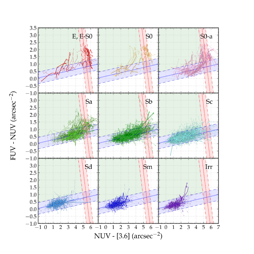
Figure 11.— (FUV $-$ NUV) vs (NUV $-$ [3.6]) spatially resolved color-color diagrams per morphological type. The regions delineated by a solid line and two parallel dashed lines are the GBS in blue and the GRS in red, and the region in green in the upper-left quadrant is the GGV, as defined in Bouquin et al. (2015). Measurements at the center are represented by triangles, and other measurements, as we move radially outward every 6″, are represented by dots connected by a line for each galaxy. Randomly selected galaxies are emphasized in each panel for better visualization.

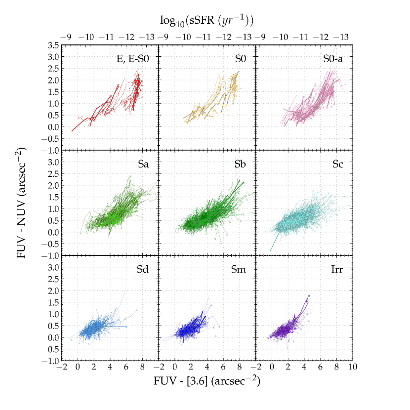
Figure 12.— (FUV $-$ NUV) vs (FUV $-$ [3.6]) spatially resolved color-color diagrams per morphological type.

4.5. GALEX Green Valley galaxies

A subsample of 70 GALEX Green Valley (GGV) galaxies was identified in the (FUV $-$ NUV) vs (NUV $-$ [3.6]) integrated color-color diagram by Bouquin et al. (2015).

As already pointed out in that paper, these objects can be interpreted as galaxies that have either left the GBS and are “transitioning” to eventually reach the GRS or were previously in the GRS and are now experiencing a modest rebirth or rejuvenation (in terms of the light-weighted ages of their stellar populations) and are evolving back to the GBS.

In the former scenario star formation would have been suppressed (or, at least, damped), either by starvation from having used up all the gas or by ram-pressure stripping, or by quenching due to the perturbations induced from AGN, merger events, or some other gas-heating process. OB stars would not form any longer and the FUV and NUV emissions decrease, with the FUV emission evolving faster than the NUV because of the shorter lifespan of the most massive stars, resulting in a progressive reddening of their (FUV $-$ NUV) color.

In the case of the latter (rejuvenation) scenario, these galaxies would have started to form stars on top of relatively passively evolving galaxies either by the accretion of new gas or by cooling gas that was already present in the galaxy in a hotter phase.

The results presented above provide another fundamental piece of evidence for the origin of these transitioning objects. In particular, we have shown that the outer parts of most GGV galaxies are redder than their inner parts and that this reddening is progressive (see, e.g., Figure 13). In the case of the quenching scenario this implies that the mechanism responsible for the quenching is acting in an outside-in fashion. Should the rejuvenation scenario be happening then these galaxies would be starting to form stars from inside-out. As the associated blue colors are not limited to the very central regions this would likely imply the growth of a disk, again, in an inside-out fashion.

With regard to the mechanism(s) that could potentially lead to the supression of the star formation in the outskirts we showed in Bouquin et al. (2015) that the GGV has the highest fraction of Virgo cluster galaxies, with 20 (out of 70) GGV objects in the Virgo cluster, i.e. $\sim$29%, in comparison to a fraction of Virgo cluster galaxies in the GBS of only $\sim$7% (124/1753) and in the GRS of $\sim$18% (14/79). For example, one ram pressure model in Virgo (Boselli et al., 2006) creates an inverted color gradient compared to late-type field galaxies, with redder outer disks and bluer inner parts.

We also analyze whether the GGV objects are mainly located in groups where environmental effects might start to occur (in particular, strangulation; Kawata & Mulchaey, 2008). Amongst the 70 GGV galaxies of our sample, 28 (40%) are field galaxies, and 42 (60%) are in groups or clusters. We see that the fraction of field galaxies decreases to 30% while the fraction of group galaxies increases to 70% (56/79) in the case of GRS galaxies. In contrast, the fraction of field/group galaxies is 51%/49% in the case of GBS galaxies, and that of the overall sample is 50%/50%. That is, we see an increase in fraction of galaxies belonging to groups as we go from the GBS to the GRS. This result hints that the disk-reddening that we see in GGV galaxies is likely due to a mechanism that is favored in dense environments. We note that this result does not exclude rejuvenation scenarios, as many ETGs with extended star formation are recently now being identified (Salim et al., 2012; Fang et al., 2012; Yıldız et al., 2017).

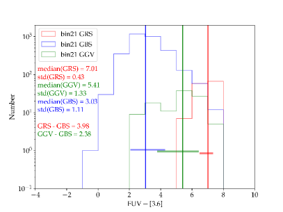
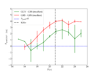
Figure 13.— Top: the number counts of data points of GBS (blue), GGV (green), and GRS (red) galaxies within a 3.6 $\mu$m surface brightness bin 21 $\leq$ $\mu_{[3.6]}$ $<$22, in the (FUV $-$ [3.6]) color versus $\mu_{[3.6]}$ surface brightness plot. Solid lines correspond to the median and the horizontal shaded area represents the extent of one standard deviation above and below the mean (not shown), all in their respective colors. Bottom: in red, the difference of the peak (FUV $-$ [3.6]) color (i.e. the difference of the median) of the GRS distribution and the GBS distribution for each $\mu_{[3.6]}$ bins. The same in green for the difference between the peaks of the distributions of GGV and GBS. The horizontal dashed blue line at $\Delta_{peak}$=0, and the vertical dot-dashed black line at $\mu_{[3.6]}$=20.892 mag arcsec^-2 of Kauffmann et al. (2006), are shown for references. Errorbars represent the 15.865 and 84.135 percentiles of the GRS and GGV distributions obtained by using the IQR method.

5. Modeling 3.6 $\mu$m exponential disks

The linear disk fits were compared to the profiles of BP00 disk models, generated with various circular velocities and spin parameters. These are simple disk models, without any bulge, bar, or mass outflow features, calibrated on the Milky Way (MW), with the assumption that our Galaxy is a typical spiral galaxy (Boissier & Prantzos, 1999) (BP99), and using simple scaling relations to extend the initial model to other spirals (BP00). These models grow inside-out with an infall of primordial gas (i.e. low-metallicity) with radially varying and exponentially decreasing infall rate with time. They include realistic yields and lifetimes from stellar evolution models and metallicity-enhancement by SNIa, and adopt a Kroupa IMF. The local SFR varies with the gas surface density and the angular velocity. The chemical and photometric evolution of the disk is then followed within this self-consistent framework. The rotational velocity, $v_{\mathrm{c}}$, is related to the total baryonic mass (Mo et al., 1998) and is implemented in a relative way with respect to the Milky Way model:

$$\frac{v_{c}}{220}=\left(\frac{M}{M_{MW}}\right)^{1/3}$$ (4)

and the dimensionless spin parameter $\lambda$ is defined as (Peebles, 1969)

$$\lambda=J|E|^{1/2}G^{-1}M^{-5/2}$$ (5)

where $M$ is the total baryonic mass, $M_{MW}$ is the total baryonic mass of the Milky Way, and 220 (km s^-1) is the circular velocity of the Milky Way, $J$ is the angular momentum, $E$ is the energy, of the halo, and $G$ is the gravitational constant. In the BP00 models, the spin parameter only influences the scalelength of the disk with respect to the MW:

$$\frac{R}{R_{MW}}=\frac{V}{V_{MW}}\frac{\lambda}{\lambda_{MW}}$$ (6)

where $R$ and $\lambda$ are the scalelength and the spin parameter of the considered model, and $R_{MW}$ and $\lambda_{MW}$ are those of the MW. We show that we are able to obtain circular velocities and spin for the galaxies of our sample from this method (Section 5.1). Finally, we show color gradients against circular velocity, spin parameter, and stellar mass of our sample (Section 5.2). In particular, gradients are positive at $\sim$50 km/s , the average is flat at $\sim$75 km/s , while above $\sim$100 km/s, most galaxies have negative gradients in all three colors.

5.1. Obtaining circular velocity and spin

In this study, we use the disk models of BP00 as in the version presented in Muñoz-Mateos et al. (2011), but increasing the sampling and range spanned by the model parameters, namely circular velocity $v_{\mathrm{c}}$ and spin $\lambda$. As mentioned above, these are bulgeless, disk-only models, that naturally grow inside-out from gas infall and are left to run for $T$=13.5 Gyr to the present. They include scaling laws so that mass scales as $v^{3}$ and scale length as $\lambda\times v$ (Mo et al., 1998). As can be seen in Figure 14, an increase in circular velocity $v_{\mathrm{c}}$ leads to an increase in both the total stellar mass and the disk scale-length, whereas increasing the spin parameter $\lambda$ only increases the scalelength. Correcting our observed galaxies for inclination (see Section 4.1) leads to a dimming in surface brightness at all radii, and thus eventually, would yield a lower circular velocity and a larger spin than when not applying the correction.

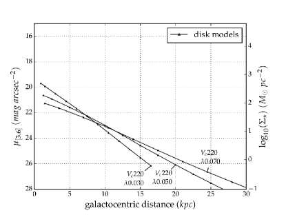
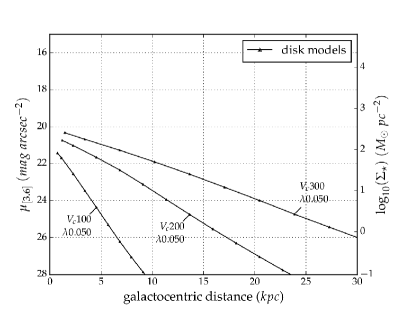
Figure 14.— Examples of 3.6 $\mu$m surface brightness profiles of BP00 disk-models with fixed circular velocity $v_{\mathrm{c}}$ and variable spin parameter $\lambda$ (top), and with fixed spin parameter and variable circular velocity (bottom).

These models are aimed to reproduce the multiwavelength SB profile by varying only those two parameters. Other assumptions were calibrated in the Milky Way model (BP99) and in nearby disks (BP00). Predictions for disks with different spins and velocities are based on $\Lambda$CDM scaling laws. Disk models were generated for various spin parameters and circular velocity combinations: the spin ranges from 0.002 to 0.15, inclusively, and varying by a step of 0.001, i.e., 149 different spins, while the velocity ranges from 20 to 430 km s^-1, inclusively, and varying by a step of 10 km s^-1, i.e., 42 different velocities. The total number of models generated is 6258. We fit these models with an error-weighted linear fit (in surface brightness scale) in a similar manner to what we do with our data points. It is, however, necessary to insert an uncertainty to the data point of each model in order to compute the reduced-$\chi^{2}$ of the fit and to determine whether an exponential law properly describes also the radial distribution of the UV through near-infrared light in these models. A reasonable assumption in this regard is 0.10 - 0.15 mag (see e.g Muñoz-Mateos et al. (2011)). Indeed, a value of 0.15 mag yields a reduced-$\chi^{2}$ close to unity for most of the models.

Figure 15 shows the slopes and $y$-intercepts obtained from the fits to the IR surface brightness profiles (corrected for inclination) of our galaxy sample plotted along with the grid of slopes and y-intercept obtained from fits to the BP00 models described above. Data errorbars are coming from the slope and y-intercept fitting errors obtained from the weighted fits to our surface brightness profiles. The errorbars in the slopes and $y$-intercepts of the models are omitted for simplicity. They are separated by morphological type.

Figure 15.— Slope (i.e. scale length) versus y-intercept (i.e. central SB) of the linear fits to the disks of the $\mathrm{S^{4}G}$ galaxies in the [3.6] micron radial profile $\mu_{[3.6]}$ (in surface brightness scale) vs kpc plane, and where the different panels correspond to different morphological types. Cutoffs for the linear fit in surface brightness scale were set at $R/R80$=0.5 and $\mu_{[3.6]}$=23.5 mag arcsec^-2. Color-coding by morphological type is the same as in the previous figures. The total number of galaxies in this plot is 987. The star marker, at $v_{\mathrm{c}}=220$ km s^-1 and $\lambda=0.03$, represents the circular velocity and spin parameter of the Milky Way and is present in all panels as reference.

This approach allows us to assign to a given galaxy disk a specific 3.6 $\mu$m central surface brightness and scale length along with the corresponding closest model. That way we are able to deduce circular velocities and spin parameters for the entire $\mathrm{S^{4}G}$ sample. In Figure 16 we show the circular velocity and spin distributions and the comparison between both parameters for the entire sample. We split these parameters by morphological type.

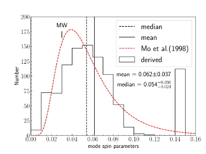
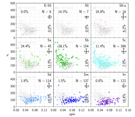
Figure 16.— Distribution of the mode of the best-fitting models circular velocity $v_{\mathrm{c}}$ (top left) and spin parameter $\lambda$ (top right) for the $\mathrm{S^{4}G}$ sample when cutoffs of $R/R80$=0.5 and $\mu_{[3.6]}$=23.5 mag arcsec^-2 are used to isolate the disk component of these galaxies’ profiles. For the spin parameter distribution, we also show the probability distribution (scaled to our distribution so that both distributions have the same area) of the spin parameter derived by Mo et al. (1998) for comparison (red). For the circular velocity distribution, we compare it with circular velocities obtained from HyperLeda (blue dashed histogram). The deduced circular velocities distribution (black solid lines) is compared with the circular velocities available in HyperLeda (blue dashed lines). The mean (solid vertical line) and the median (dashed vertical line) positions are shown for each distribution, annotated with the value and the 1-$\sigma$ uncertainty. The circular velocity plotted against the spin parameter, split by morphological type, is shown in the bottom panel. Average uncertainties are shown in the top-right corner. The Milky Way (MW) values are shown in both panels. Open circles indicate galaxies that have extreme values, either in circular velocity or in spin parameter, or both, and are shown using their central value instead. The percentage shown in the upper-left is the fraction of outliers in $v_{\mathrm{c}}$, whereas the one shown to in the lower-right and rotated is the fraction of outliers in spin parameters. Outliers in both $v_{\mathrm{c}}$ and spin are included in both fractions.

For each pair of best-fitting slope (i.e. scale-length) and y-intercept (i.e. central surface brightness) measurements we generated a thousand random points using elliptical 2D-gaussian probability distribution functions with the 1-$\sigma$ being the uncertainties in these measurements and obtained the closest model for each Monte-Carlo particle. Thus, for each data point (i.e., for each galaxy) we obtained a distribution in best-fitting circular velocity and spin parameter. Typical distributions of circular velocities from the sampling of 1000 points are shown in Figure 17. This figure also shows the distribution of the individual 1000 points in the circular velocity versus spin diagram for three example galaxies. There is a mild degeneracy between the two parameters (although we show galaxies with very skewed distributions) in some of these objects that is in the same direction as the correlation seen in Figure 16 for late type galaxies. Note, however, that such correlation is not driving the whole distribution of points in Figure 16 and that the latter spans a wider range of spins and circular velocities than the 1$\sigma$ errors found for the individual galaxies. Thus, although the degeneracy between the two parameters certainly contributes to the morphology of the different panels of Figure 16, it also reflects the bona fide distribution of physical properties of the disks of galaxies in the Local Universe.

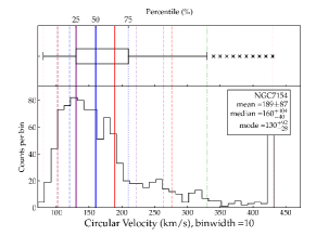
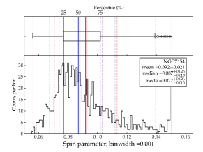
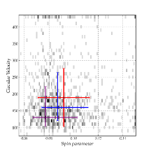
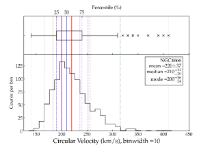
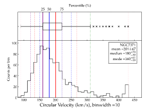
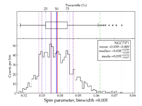
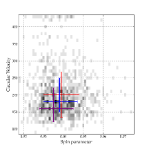
Figure 17.— Examples of typical circular velocities $v_{\mathrm{c}}$ (left column) and spin parameters $\lambda$ (middle column) distributions (namely NGC7154, NGC4666, and NGC7371 that are classified as Sm, Sc, and S0-a galaxies, having absolute AB magnitude $\mathrm{M}_{[3.6]}=-19.62$, $-21.90$, and $-20.77$ mag) for a sampling of 1000 slope and y-intercept values. The plots in the right column show the distribution of the 1000 simulated MC particles in circular velocity versus spin. The spin and circular velocity mean, median, and mode values and corresponding derived errors (assuming the two quantities are derived separately) are also shown. The red solid line is the mean, the red dashed lines are $\pm 1\sigma$ from the mean, the blue solid line is the median, the blue dashed lines are $\pm 1\sigma$ from the median (15.865% and 84.135% lower and upper percentiles), the blue dotted lines are Q1 (25%) and Q3 (75%), the green dot-dashed lines are Q1-1.5$\cdot$IQR and Q3+1.5$\cdot$IQR, where IQR is the interquartile range Q3 - Q1, and the pink dashed lines are the distribution’s range. Crosses are used to show the bins that were excluded when computing the percentiles.

We see that this method of sampling produces circular velocity distributions with long tail towards high $v_{\mathrm{c}}$. These asymmetric distributions, for which the median or the mode give a better estimate of the peak of the distribution (rather than the mean) for the corresponding parameter, are a consequence of the non-regularity of the coverage of the model grid in Figure 15. In this work, we make use of the mode values and the percentiles obtained from these distributions to get the data points and average errorbars in Figure 16. We also list the results obtained in Table 9.

Table 9GALEX/$\mathrm{S^{4}G}$ sample circular velocity and spin obtained from a grid of BP00 disk models

galaxy name	$v_{\mathrm{c}}$	$\lambda$	T
ESO293-034	130${}^{+40}_{-28}$	0.041${}^{+0.008}_{-0.007}$	6.2
NGC0024	110${}^{+13}_{-27}$	0.027${}^{+0.003}_{-0.006}$	5.1
ESO293-045	90${}^{+24}_{-16}$	0.066${}^{+0.009}_{-0.009}$	7.8
UGC00122	70${}^{+15}_{-25}$	0.067${}^{+0.008}_{-0.007}$	9.6
NGC0059	50${}^{+...}_{-...}$	0.032${}^{+0.004}_{-0.004}$	-2.9
ESO539-007	110${}^{+25}_{-45}$	0.150${}^{+...}_{-0.029}$	8.7
ESO150-005	110${}^{+45}_{-35}$	0.150${}^{+...}_{-0.033}$	7.8
NGC0115	130${}^{+41}_{-29}$	0.044${}^{+0.010}_{-0.007}$	3.9
UGC00260	430${}^{+...}_{-288}$	0.070${}^{+0.023}_{-0.012}$	5.8
…

.

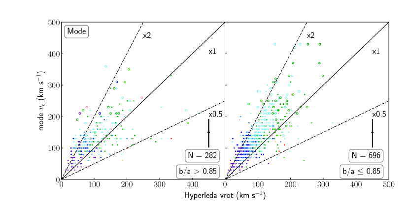
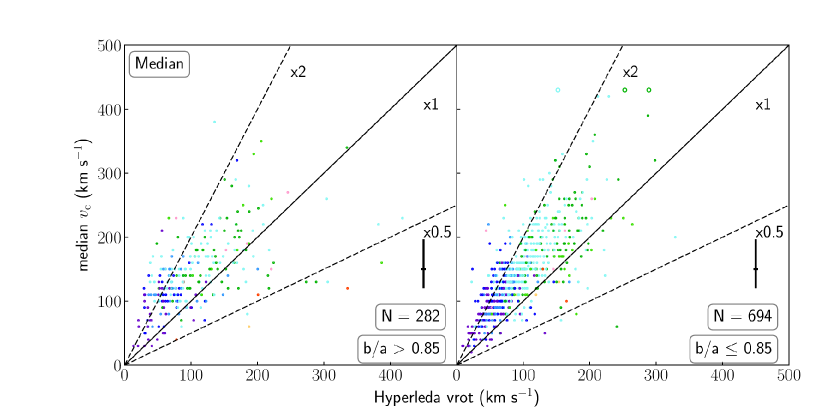
Figure 18.— Rotational velocity $v_{\mathrm{c}}$ obtained from BP00 grid models for our sample galaxies once the $\mu_{[3.6]}$ profiles are corrected for inclination compared to the maximum rotational velocity obtained from HyperLeda (corrected for inclination) $v_{\mathrm{rot}}$. The 1:1 and 2:1 & 1:2 ratios are shown as dashed lines as visual guides. Here, we use the mode (top) and median (bottom) of $v_{\mathrm{c}}$ obtained for each galaxy (see Figure 17). We distinguish between galaxies of high and low inclination using the minor-to-major axis ratio $b/a$ ($\leq 0.85$ for highly inclined galaxies in the left panel, and $0.85<b/a\leq 1$ for low-inclination galaxies in the right panel). Both axes are in units of km s^-1. Open circles indicate galaxies that have extreme values, as in Figure 16, and for which we use their central value. We do not take their uncertainties into account for the computation of the average uncertainties.

We then compare our values with observed values of the circular velocity for galaxies for which we have data (see Figure 18). We obtained the inclination-corrected maximum rotational (i.e., circular) velocity and its associated uncertainty from HyperLeda, vrot and e_vrot. These observed values are computed from the apparent maximum rotation velocity obtained from the width of the 21 cm line at various levels, or from H$\alpha$ rotation curves. They are homogenized using a large sample ($>$50000) of measurements and are corrected for inclination (Paturel et al., 2003). We do not aim here to provide a fully coherent set of circular velocity measurements but to see whether or not the values that we obtain from our method are similar to the observed ones. In the case of our ‘best’ $\chi^{2}$ fit with cutoffs of $R/R80$ $\simeq$ 0.5 and $\mu_{[3.6]}$ $\simeq$ 23.5 mag arcsec^-2, 976 galaxies when using the median, and 978 when using the mode out of 987 have actual measurements in HyperLeda. In the case of the mode, we quantify the 1-$\sigma$ (68.269%) distribution range to the left (right) of the mode by counting only the bins on the left-hand-side (right-hand-side) distribution starting from the bin of the mode, but excluding it from the counts. Also, in case of multimodal distributions, we chose the bin with the smallest associated value. When we compare the two, we see that most of our values are larger than the observed ones, but rarely above twice the observed rotational velocity. This effect comes partly from the accuracy of extracting the peak value over the skewed distributions of the circular velocities and spin parameters that we obtained from our method as can be seen in Figure 18. When the distribution is skewed to the left, the mean is systematically larger than the median, and the median is larger than the mode, and vice-versa when the skew is to the right, then the mean is smaller than the median, and the median is smaller than the mode. This comes from our grid of models (Figure 15) and the sampling that we use to extract the best model. For given observational uncertainties and as the slope flattens out, higher circular velocity models that match the observations largely increase. The same holds true for larger values for the y-intercept (i.e., fainter): the higher the spin, the more models that match the observations. Hence the sampling distributions show a tail toward larger circular velocities and spin parameters. Using either the median or the mode gives similar results. This is shown in Figure 18 where using the median yields a similar scatter that when using the mode.

Our values are consistent with the observed values within a factor of 0.5 to 2, especially if the very large uncertainties present are taken into account. The distributions given in Figures 16 provide powerful tools to test the predictions for numerical simulations of disks in a cosmological context.

5.2. Color Gradient versus circular velocity, spin, and stellar mass

Finally, we compare the color gradients (the slopes) obtained in the (FUV $-$ NUV), (FUV $-$ [3.6]), and (NUV $-$ [3.6]) color profiles (with a cutoff at $R/R80$=0.5 but no cutoff in SB; see Table 6) against the mode circular velocities, mode spins that we derived with the method described in Section 5.1, and stellar masses calculated from the 3.6 $\mu$m SB. This is shown in Figure 19. The panels showing the circular velocity and spin comprises 987 galaxies, whereas the panels showing the stellar mass comprises 1541 galaxies. For the mode circular velocities, a large scatter is seen especially for low-mass systems, in all three colors. In the case of the mode spin parameters, the scatter is very much the same throughout the entire range of spins, for all morphological types, and for all three colors. Then, the color gradient versus the stellar mass plots show a large scatter for low-mass galaxies with stellar mass of around 10⁸–10⁹ M_⊙. On average, there is a trend toward more negative gradient as we move to larger masses, and therefore indicating bluer outer disks. However, most low-mass galaxies and a non-negligible fraction of massive galaxies show positive color gradients.

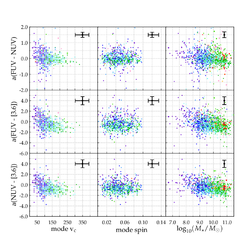
Figure 19.— Color gradients (slopes of least-square linear fit) in the (FUV $-$ NUV), (FUV $-$ [3.6]), and (NUV $-$ [3.6]) colors versus circular velocities (mode), spins (mode), and stellar masses, respectively. A positive color gradient indicates a reddening as we move to the outskirts. A negative color gradient indicates a blueing. Average 1-$\sigma$ uncertainties in both axes are shown in the upper-right corner of each panel.

6. DISCUSSION

We discuss here about circular velocity and spin of galaxies in the local Universe in Section 6.1. It is crucial to understand where this UV emission is coming from within the galaxies (Section 6.2). In this regard, an important point that needs to be addressed is the fact that the UV emission not only comes from newly born massive stars, but also from evolved low-mass stars. We also discuss galaxy evolution and the effects of the environment on populating the green valley (Section 6.3).

6.1. Circular velocity and spin of galaxies in the local Universe

The results shown in Section 5 show that it is possible to derive (albeit with relatively large uncertainties in specific cases) the statistical distribution of circular velocity (total mass) and spin (specific angular momentum) of galaxies from the analysis of deep near-infrared photometry of their disks. Besides, the fact that we can impose some simple criteria to isolate the disk component of the profiles makes this kind of analysis a very powerful tool for its application to upcoming surface photometry data from LSST, EUCLID or WFIRST.

Our analysis reveals that up to the current surface brightness detection limits (we note that all $\mathrm{S^{4}G}$ galaxies are detected by Spitzer but many low-surface brightness objects might still be missing from the catalogs) nearby galaxies show a wide distribution in spin with a maximum at $\lambda$$\sim$0.06 and a relatively high fraction (24%) of galaxies with $\lambda$$>$0.08 (see top-right panel of Figure 16).

The comparison of these values with those derived for the SINGS sample (Kennicutt et al., 2003) by Muñoz-Mateos et al. (2011) using a similar method and a similar set of models indicate a larger number of high-$\lambda$ systems in our sample, in terms of the mean, median, and mode of the distribution. This is expected in the case of the SINGS sample as this is biased towards high surface brightness systems with low angular momentum content relative to their mass. In addition, the SINGS sample (75 galaxies) was constructed to sample physical parameters (morphological type, luminosity, and FIR/optical luminosity ratio) and therefore, is not representative in numbers of different kind of galaxies. With respect to the predictions of semi-analytic models (e.g., Mo et al., 1998), we find a median value that is displaced towards larger spins (0.06) relative to recent simulations ($\sim$0.036, quite independently of the galaxy mass and method of determining $\lambda$; Rodríguez-Puebla et al., 2016). To quantify this distribution, for the $\mathrm{S^{4}G}$ sample we derive mean (with 1-$\sigma$ distribution width) and median values of 0.062$\pm$0.037, 0.054${}^{+0.030}_{-0.024}$, respectively, while, for Milky Way mass halos, the models of Rodríguez-Puebla et al. (2016) yield a mean of 0.036 with a dispersion of 0.24 dex (for the spin parameter $\lambda_{P}$ of Peebles, 1969).

With regard to the circular velocities, we find a relatively narrow mode distribution peaking at 120$\sim$$v_{\mathrm{c}}$$\sim$149 km s^-1 (ignoring the outliers.) (top-left panel of Figure 16). This indicates a lack of low-mass (dwarf) systems, which is probably occurring both at the high surface brightness (because of our diameter selection for $\mathrm{S^{4}G}$) and low surface brightness ends (because of the limiting central surface brightness present in the catalogs of nearby galaxies). Determining a volume- and diameter-corrected circular velocity (i.e., halo mass) function is beyond the scope of this paper. It could, however, be an interesting test for the models complementary to the halo mass functions derived from dynamical masses obtained from the modeling of 21 cm velocity maps and line profiles (de Blok et al., 2008; Papastergis et al., 2013) (see also Zaritsky et al., 2014b, which connected the kinematics to the baryon fractions using the $\mathrm{S^{4}G}$).

Finally, the distribution of circular velocity vs spin (bottom panel of Figure 16) shows a larger dependence of the spin on the circular velocity than that found by Rodríguez-Puebla et al. (2016). In those cases where the data point, or a significant portion of the input probability distribution of the y-intercept and slope of the 1000 sampled points, is outside of the grid, the mode is biased towards the maximum value models in spin or circular velocity, or both, we use the central value instead of the mode value. These are shown as open circles. The percentages are the fractions of outliers in circular velocity (top-left) and spin parameter (bottom-right). Outliers in both parameters are included in both fractions. Uncertainties for the outliers are not included in the average uncertainty. The lack of objects of high spin and low circular velocity could be due to the surface brightness limit involved in defining our sample. However, this would make our distribution even wider towards high-$\lambda$ values (see also Mo et al., 1998). Besides, the lack of low-mass, low-spin galaxies (high surface brightness dwarfs) is attributable to our diameter selection ($>$1 arcmin), as these would be very compact dwarf systems.

Thus, we conclude that the strong dependence of the spin on the circular velocity and, in particular, the lack of low-mass galaxies at both extremes of the distribution in spin, might be due to selection effects in the $\mathrm{S^{4}G}$ survey (at least we cannot conclude otherwise). The relatively flat distribution of spin values in the range between $\lambda$=0.03-0.11, which would be even more extended towards high-$\lambda$ values, used to pose a challenge to current models of galaxy formation. However, Amorisco & Loeb (2016) have recently shown that the properties and abundances in clusters of large, ultra-diffuse galaxies (UDGs) can be reproduced from within a standard cosmological framework and classical disk-formation models. It will be interesting to see, once catalogs of low-surface brightness disk galaxies will be available (including UDGs such as those found by Koda et al., 2015, in Coma) how they are distributed in terms of spin and circular velocity.

6.2. Radial distribution of UV emission: UV-upturn and star formation

The UV emission found in the 1931 galaxies within the $\mathrm{S^{4}G}$ sample is clearly aligned in two sequences of UV-to-IR colors. These two sequences, which are called the GALEX Red (GRS) and Blue (GBS) sequences and which are best isolated in the (FUV $-$ NUV) and (NUV $-$ 3.6 $\mu$m) color-color diagram and when galaxies are previously split by morphological type (see Figure 11), correspond each to a different mechanism responsible for the UV emission. In the case of the GRS, the big change in (FUV $-$ NUV) color ($\sim$1.5 mag) with a change in (NUV $-$ 3.6 $\mu$m) of $<$1 mag can only be attributed to the UV-upturn phenomenon (O’Connell, 1999), which is believed to be caused by very hot EHB stars (see Zaritsky et al., 2015, and references therein).

On the other hand, the GBS has a slope of 0.12 (see Equation 1), which implies a change of only 1.2 mag in the (FUV $-$ NUV) color for a change of 10 mag in (NUV $-$ 3.6 $\mu$m). As shown in Bouquin et al. (2015) this slope agrees well with the color correlation predicted by spectro-photometric models for the evolution of galaxy disks (see, e.g., BP00), so the UV emission of these objects can be interpreted as due to emission from relatively massive stars in the turn-off of the main sequence.

The GRS is mainly populated by E, E-S0, S0 and S0-a morphological types and it is clearly isolated in its (FUV $-$ NUV) blue end only in ETGs, i.e., E, E-S0 and S0 galaxies. This isolation is possible thanks to the dichotomy in the (NUV $-$ 3.6 $\mu$m) colors of the central regions of ETGs (triangles in Figure 11). They are either very blue, indicating (residual) star formation in these innermost regions, or very red, which points towards a very old (light-weighted) stellar population. The fact that these very old populations in the centers of ETGs are also the ones showing the strongest UV-upturn is something that has been explained in the past as being related to either the older age or higher metal (helium, at least) abundance of the horizontal branch stars responsible for the UV emission in these regions (Boselli et al., 2005), but may also be tied to the observations supporting differences in IMF (e.g. Conroy & van Dokkum, 2012; Cappellari et al., 2012, 2013a, 2013b).

In early-to-intermediate spirals (S0-a through Sc) the central regions of many galaxies appear in the locus where the GBS and GRS overlap. Besides, the entire GBS is well populated by measurements obtained both in the inner and outer regions of galaxies. Thus, these colors are of no use to determine whether the UV emission from the bulges of these galaxies are dominated by emission from young massive or evolved low-mass EHB stars or by a combination of both. Both the outer parts of early-to-intermediate spirals (except for regions populating the GGV; see below) and the late-type spirals (Sd and beyond) at all radii follow a narrow GBS. According to the color profiles shown in Figure 3, the majority of the galaxies that are found to populate the GBS show negative color gradients, which is in agreement with the global scenario of inside-out formation of their disks. The study of the most extreme cases of inside-out disk formation will be the subject of a future communication. At the surface brightness levels reached by our data we do not find clear signs of color upbending, at least in the bands considered in this work (see Bakos et al., 2008; Marino et al., 2016, for studies of reversed optical color profiles and ionized-gas chemical abundance gradients in outer disks).

Finally, it is also worth mentioning that the central regions of galaxies (despite having the highest signal-to-noise ratios) show the widest dispersion in all three (FUV $-$ NUV), (FUV $-$ 3.6 $\mu$m) and (NUV $-$ 3.6 $\mu$m) colors among galaxy types and as a whole, covering $\sim$10 mag in the case of the latter two colors. This, of course, indicates that nuclear regions are the least homogeneous within the population of local galaxies in terms of their stellar population and dust content.

6.3. Galaxy evolution through the Green Valley

Here we focus on discussing the properties of those galaxies that were identified in Bouquin et al. (2015) as being globally included in the so-called GALEX Green Valley and also of those regions within galaxies that are now found to be located in the GGV even though they are part of the GBS or GRS when considered as a whole.

In Figures 7 and 8 we showed that galaxies that belong (globally) to the GGV are mainly lenticulars and early-type spirals (S0-a through Sb), showing a relatively narrow distribution of (observed) sSFR around 10^-12 yr^-1. Furthermore, Figure 9 shows that the outer regions of GGV galaxies behave differently from the outer regions of most GBS systems, with the FUV$-$3.6 $\mu$m color getting redder as we move progressively towards their outer disks. This clearly indicates that the reason why these objects are in the GGV is that their disks are redder, for the same morphological type and surface brightness, than those of most GBS galaxies. Exploration of Figure 9 in the case of the GBS shows that the region of red disks is populated by a number of ETGs with profiles similar in shape to those found in the GRS but that they probably show a very blue nucleus that places them in the GBS when considered as a whole.

A small fraction of GBS galaxies (mainly early-type spirals, but only a fraction of them) have disks that also redden with radius. These are objects that are likely to evolve into GGV galaxies or objects which GGV galaxies will evolve into, depending on whether GGV galaxies are quenching their star formation or regrowing a disk.

Our analysis shows that the fraction of galaxies belonging to dense environments is higher for GGV galaxies than for GBS galaxies, but is less than for the GRS. This result, combined with the fact that GGV galaxies have redder outer disks, hints at the direction of the evolution, from GBS to GRS, which favors star formation quenching due to environmental effects. Similar results have been obtained in the analysis of galaxies in clusters (see Wolf et al., 2009; Bamford et al., 2009; Cibinel et al., 2013; Head et al., 2014).

Moreover, a study of galaxies in transition in different environments (Vulcani et al., 2015) shows that galaxies in groups have a higher quenching efficiency than field galaxies. Their results show that color transformation is due to the overall decrease in SFR, both in bulges and disks, while maintaining the morphology. They also show that morphological transformation is due to an increase in bulge-to-disk ratio because of disk removal, and not because of the growth of the bulge, in disagreement to a bulge enhancement and absence of disk-fading scenario (Christlein & Zabludoff, 2004). What is presented in Section 4 is in agreement with the former, where disk-fading occurs, resulting in an increase in the bulge-to-disk ratio.

7. SUMMARY AND CONCLUSIONS

We have gathered GALEX FUV and NUV images for the $\mathrm{S^{4}G}$ sample, and have measured their FUV and NUV magnitudes. Our UV subsample comprises 1931 galaxies, and has an identical distribution in morphological type, distance, and 3.6 micron absolute magnitude as the $\mathrm{S^{4}G}$ sample of 2352 galaxies (Figure 1). Our GALEX subsample is compatible with being a random subsample of the entire $\mathrm{S^{4}G}$ sample, and can also be considered as representative of the local universe.

The photometry is done within rings with fixed PA and $\epsilon$ at every 6$\arcsec$ steps in semi-major axis length and with width of 6$\arcsec$. The products are the $\mu_{\mathrm{FUV}}$ and $\mu_{\mathrm{NUV}}$ surface brightness profiles, (FUV $-$ NUV) color profiles, along with the asymptotic FUV and NUV magnitudes and (FUV $-$ NUV) color. Data are partially summarized in Table 1, and the full catalog is available online. We have generated RGB postage-stamp images from UV images only, and also obtained the $\mu_{\mathrm{FUV}}$, $\mu_{\mathrm{NUV}}$ surface brightness, as well as the (FUV $-$ NUV) color profiles. We used the RC2 numerical morphological classification to roughly classify the galaxies into narrower morphological type bins (sample demographics are summarized in Table 2).

These UV products, combined with the near-IR products of the $\mathrm{S^{4}G}$ sample, form an excellent set of tools to probe nearby galaxies, as we are directly tracing the current SFR with the former and the stellar mass with the latter, thus the sSFR. We have thus characterized the radial distributions of young and old stars in galaxies in the local Universe.

We also looked at the spatially resolved colors formed by the three bands. The (FUV $-$ NUV) color is most suitable for detecting variations in recent star formations on time-scales below 1 Gyr. The (FUV $-$ [3.6]) color is equivalent to a measurement of the observed sSFR. The (NUV $-$ [3.6]) color is useful to construct the (FUV $-$ NUV) vs (NUV $-$ [3.6]) color-color diagram, in which the GALEX Blue Sequence (GBS) and GALEX Red Sequence (GRS) subsamples are defined in the preliminary analysis of Bouquin et al. (2015). We see that the galaxies are grouped into narrow sequences in this color-color diagram, and do separate very well between star-forming (GBS) and quiescent (GRS) galaxies. This allowed us to define an intermediate region, the GALEX Green Valley (GGV), where we find galaxies that are either leaving the blue sequence due to some damping of their star formation activity, or leaving the red sequence possibly by rejuvenation. We also performed the fit in the color profiles, and show the distributions of the resulting slopes and $y$-intercepts (scale length and central SB of disks).

Our main results are the following:

- GBS, GGV, and GRS galaxies are well separated in the $\mu_{\mathrm{FUV}}$ vs $\mu_{[3.6]}$ plane. Most disks are located in a well defined sequence which we call the “spatially resolved main-sequence of star-forming disks”, with 3.6 micron surface brightness ranging from 20 to 25 mag arcsec^-2, and FUV surface brightness ranging from 24 to 27 mag arcsec^-2. The GBS galaxies are dominating the highest surface sSFR densities, while the GRS galaxies are dominating the lowest surface sSFR density. The early-type galaxies of the GRS have a low surface sSFR density, $\Sigma_{\mathrm{sSFR}}$, that stays radially constant at (or below) 10^-12 yr^-1 pc^-2. The late-type galaxies of the GBS, on the other hand, have higher surface sSFR densities the later the type, with increasing surface sSFR density (blueing) inside-out. This is not always the case, since inside-out disk reddening is also seen for some of the galaxies. This reddening translates to sudden drops in surface SFR density, and indicates a possible quenching (or damping; see Catalán-Torrecilla et al., 2017) of the star formation in the outskirts.

- Star-forming GBS, quiescent GRS, and intermediate GGV galaxies are well separated in the (FUV $-$ [3.6]) vs $\mu_{[3.6]}$ plane, especially when one looks at the colors of the isophote that encompasses 80% of the 3.6 $\mu$m light (equivalent to the same percentage of stellar mass). The isophotes of the GGV galaxies fill the gap between the locus of the GBS and the GRS ones. Particularly, most GRS galaxies show very similar radial behavior to each other, and most of them end up in a similar locus in the (FUV $-$ [3.6]) vs $\mu_{[3.6]}$ plane, where the 80% enclosed-light isophote ends up in a narrow range in 3.6 $\mu$m surface brightness, between 21 and 23 mag arcsec^-2, and in (FUV $-$ [3.6]) color range between 6 and 7 mag.

- We performed an analysis of the 3.6 $\mu$m surface brightness radial profiles by linearly fitting the data points using an array of cutoffs both in radial distance and in 3.6 $\mu$m surface brightness, to approximately exclude the bulge part and only fit the disk part. We find the best cutoffs values to be $R/R80$ = 0.5 and $\mu_{[3.6]}$ = 23.5 mag arcsec^-2 (corresponding to a stellar mass surface density of $3\times 10^{7}$ $M_{\odot}$ kpc^-2), where the mean reduced-$\chi^{2}$ approaches unity and the number of galaxies is maximized ($>$50% of the sample). Doing so, we efficiently excluded the bulge parts, as well as massive galaxies, and obtained a subsample of 987 disk galaxies for further analysis. These slope and y-intercept of the linear fit translates to circular velocities and central surface brightness (of the disk).

- Finally, we compared the slope and y-intercept of the linear fit to the outer disk parts of our subsample to the slope and y-intercept of the linear fit to of over 6258 simulated disk models of BP00 varying based on the circular velocity $v_{\mathrm{c}}$ and the spin parameter $\lambda$, thus obtaining a fine grid of slopes (i.e. scale length) and $y$-intercepts (i.e. central surface brightness). From this, we deduced the circular velocity for each of our galaxies by finding the closest model matching the slope and the y-intercept of the galaxy. We find a distribution for the mode circular velocity with mean $v_{\mathrm{c}}=149\pm 102$ km s^-1 (standard deviation 1$\sigma$) and median $v_{\mathrm{c}}=120^{+70}_{-40}$ km s^-1 (1$\sigma$ with IQR method and thus, excluding the outliers), and a distribution for the mode spin parameter with mean $\lambda=0.062\pm 0.037$ (standard deviation 1$\sigma$) and median $\lambda=0.054^{+0.030}_{-0.024}$ (1$\sigma$ with IQR method). For the spin, we recover the probability distribution function of Mo et al. (1998), whereas for the circular velocity, our distribution is skewed towards higher circular velocities than the ones obtained from HyperLeda. The low-mass Sd, Sm, and Irr galaxies seems to be more affected than larger spiral galaxies. Despite the large scatter, this method yields circular velocities similar to those observed within a range of factors of one to two for most galaxies.

Appendix A Appendix A

A.1. Deriving $\Sigma_{\star}$ from $\mu_{[3.6]}$

In this work, we make use of the stellar mass surface density $\Sigma_{\star}$ (solar mass per square parsec) distribution that is obtained from the 3.6 micron surface brightness (AB mag per square arcsec) radial profiles. We start from the definition of absolute magnitude:

$$\mathrm{M}_{[3.6],\star}=\mathrm{M}_{[3.6],\odot}-2.5\log_{10}\left(\frac{L_{[3.6],\star}}{L_{[3.6],\odot}}\right)$$ (A1)

where $\mathrm{M}_{[3.6],\star}$ and $L_{[3.6],\star}$ are the 3.6 $\mu$m absolute magnitude (AB) and luminosity (in $ergs\cdot s^{-1}Hz^{-1}$) of the galaxy, $\mathrm{M}_{[3.6],\odot}$ and $L_{[3.6],\odot}$ are the solar 3.6 $\mu$m absolute magnitude and luminosity.

We also need the following expression for the mass-to-light ratio:

$$\frac{M_{\star}}{L_{[3.6],\star}}=\Upsilon_{[3.6]}$$ (A2)

where the mass-to-light ratio of the Sun ($M_{\odot}/L_{[3.6],\odot}$) is unity, and where $M_{\star}$ is the stellar-mass of the galaxy, $L_{[3.6],\star}$ is the luminosity at 3.6 $\mu$m, $M_{\odot}$ is a solar mass, and $L_{\odot,3.6}$ is the solar luminosity at 3.6 $\mu$m. $\Upsilon_{[3.6]}$ is the mass-to-light ratio at 3.6 micron as obtained by Meidt et al. (2014) and is equal to 0.6 (assuming a Chabrier IMF).

Rearranging eq.A1 we have:

$$\frac{L_{[3.6],\star}}{L_{[3.6],\odot}}=10^{-0.4(\mathrm{M}_{[3.6],\star}-\mathrm{M}_{[3.6],\odot})}$$ (A3)

Rearranging eq.A2, and adding the conversion factor $a_{\mathrm{IMF}}$ for the transformation from a Chabrier IMF (Chabrier, 2003) to Kroupa IMF (Kroupa, 2001), we get:

$$\frac{M_{\star}}{M_{\odot}}=\frac{L_{[3.6],\star}}{L_{[3.6],\odot}}\cdot\Upsilon_{[3.6]}\cdot a_{\mathrm{IMF}}$$ (A4)

where we use, in our case, $a_{\mathrm{IMF}}=\frac{M/L(Kroupa)}{M/L(Chabrier)}=1.034$ (conversion factors from Madau & Dickinson (2014)).

We then take the log of eq.A4, combined with eq.A3:

$$\log_{10}\left(\frac{M_{\star}}{M_{\odot}}\right)=\log_{10}\left(\frac{L_{[3.6],\star}}{L_{[3.6],\odot}}\right)+\log_{10}(\Upsilon_{[3.6]}\cdot a_{\mathrm{IMF}})$$ (A5)

i.e.

$$\log_{10}\left(\frac{M_{\star}}{M_{\odot}}\right)=0.4(\mathrm{M}_{[3.6],\odot}-\mathrm{M}_{[3.6],\star})+\log_{10}(\Upsilon_{[3.6]}\cdot a_{\mathrm{IMF}})$$ (A6)

Finally, changing $\mathrm{M}_{[3.6],\star}$ to $\mu_{[3.6]}\mathrm{(AB\,mag\,arcsec^{-2})}+5-5\log_{10}d(\mathrm{pc})$ and converting arcsec^-2 to parsec^-2 gives

$$\Sigma_{\star}(M_{\odot}\,\mathrm{pc^{-2}})=\Upsilon_{[3.6]}\cdot a_{\mathrm{IMF}}\cdot 10^{0.4\mathrm{M_{[3.6],\odot}}}\cdot 10^{-0.4\cdot\left(\mu_{[3.6]}+5-5\log_{10}d\right)}\cdot\left(\frac{206265}{d}\right)^{2}$$ (A7)

where $\mathrm{M_{[3.6],\odot}}$ is the Sun’s 3.6 micron absolute AB magnitude which is taken to be 6.03 mag (converted to AB scale from the Vega magnitude value, $M_{\odot,3.6,Vega}=3.24$, given by equation(13) in Oh et al. (2008)).

This corresponds to a stellar mass surface density $M_{\star}$/area = 1.045 $M_{\odot}$/pc² at a 3.6 micron surface brightness $\mu_{[3.6]}$ = 27 mag arcsec^-2 in the case of a Chabrier IMF, and $M_{\star}$/area = 1.080 $M_{\odot}$/pc² in the case of a Kroupa IMF. The equation, then, simplifies to the following:

$$\log_{10}(\Sigma_{\star}(M_{\odot}\,\mathrm{pc^{-2}}))=10.819-0.4\mu_{[3.6]}+\log_{10}a_{\mathrm{IMF}}\\$$ (A8)

where the term $\log_{10}a_{\mathrm{IMF}}=0$ for a Chabrier IMF, $0.015$ for a Kroupa IMF, and $0.215$ for a Salpeter IMF.

Appendix B Appendix B

B.1. Deriving the observed sSFR from (FUV $-$ [3.6])

We start with the SFR(UV), assuming a Salpeter IMF (Salpeter, 1955) and using a calibration by Madau et al. (1998), as provided by Kennicutt (1998), which we can convert to the expression for a Kroupa IMF by multiplying by $b_{\mathrm{IMF}}=0.67$, or by $b_{\mathrm{IMF}}=0.63$ for a Chabrier IMF, as reviewed and prescribed in Kennicutt & Evans (2012); Madau & Dickinson (2014):

$$\mathrm{SFR}(M_{\odot}\,yr^{-1})=1.4\times 10^{-28}\cdot b_{\mathrm{IMF}}\cdot L_{\nu}\,\mathrm{(ergs\cdot s^{-1}Hz^{-1})}$$ (B1)

and with the following expression of luminosity:

$$L_{\nu} =4\pi(d(\mathrm{cm}))^{2}f_{\nu}$$ (B2)

$$L_{\nu} =4\pi\left[d(\mathrm{pc})\cdot 3.086\times 10^{18}\mathrm{(cm/pc)}\right]^{2}10^{-0.4(\textrm{FUV}+48.6)}$$

Combining the two equations above gives:

$$\log_{10}(\mathrm{SFR})(M_{\odot}\,yr^{-1})=2\log_{10}d(pc)-0.4\,\mathrm{FUV}-9.216+\log_{10}b_{\mathrm{IMF}}$$ (B3)

where FUV is in AB magnitudes, distance d is in parsec, and $\log_{10}b_{\mathrm{IMF}}=0$, $-0.174$, and $-0.201$ for a Salpeter, Kroupa, and Chabrier IMF respectively.

Secondly, we need to introduce the distance modulus $m-M=5-5\log_{10}d(pc)$ into eq. A6, so this becomes:

$$\log_{10}\left(\frac{M_{\star}}{M_{\odot}}\right)=\log_{10}(\Upsilon_{3.6}\cdot a_{\mathrm{IMF}})-0.4([3.6]+5-5\log_{10}d-6.03)$$ (B4)

where $[3.6]$ is the apparent AB magnitude at 3.6 $\mu$m, $d$ is the distance in parsec, and $M_{\odot,3.6,AB}=6.03$ (see Appendix A).

Finally, we combine B3 and B4:

$$\log_{10}(\mathrm{sSFR})=\log_{10}\left(\frac{\mathrm{SFR}}{M_{\star}}\right)=\log_{10}(\mathrm{SFR})-\log_{10}(M_{\star})$$ (B5)

It thus becomes:

$$\log_{10}(\mathrm{sSFR})=-0.4(\mathrm{FUV}-[3.6])-9.628+\log_{10}b_{\mathrm{IMF}}-\log_{10}(\Upsilon_{3.6}\cdot a_{\mathrm{IMF}})$$ (B6)

We can thus obtain the logarithm of the specific star formation rate (in units of $year^{-1}$) from the (FUV $-$ [3.6]) (ABmag) color. We emphasize that these quantities would not be corrected for extinction.

References

- Amorisco & Loeb (2016) Amorisco, N. C., & Loeb, A. 2016, MNRAS, 459, L51
- Andrae et al. (2010) Andrae, R., Schulze-Hartung, T., & Melchior, P. 2010, ArXiv e-prints
- Astropy Collaboration et al. (2013) Astropy Collaboration, Robitaille, T. P., Tollerud, E. J., et al. 2013, A&A , 558, A33
- Bakos et al. (2008) Bakos, J., Trujillo, I., & Pohlen, M. 2008, ApJL , 683, L103
- Bamford et al. (2009) Bamford, S. P., Nichol, R. C., Baldry, I. K., et al. 2009, MNRAS, 393, 1324
- Boissier & Prantzos (1999) Boissier, S., & Prantzos, N. 1999, MNRAS, 307, 857
- Boissier & Prantzos (2000) —. 2000, MNRAS, 312, 398
- Boselli et al. (2006) Boselli, A., Boissier, S., Cortese, L., et al. 2006, ApJ , 651, 811
- Boselli et al. (2005) Boselli, A., Cortese, L., Deharveng, J. M., et al. 2005, ApJL , 629, L29
- Bouquin et al. (2015) Bouquin, A. Y. K., Gil de Paz, A., Boissier, S., et al. 2015, ApJL , 800, L19
- Buta et al. (2015) Buta, R. J., Sheth, K., Athanassoula, E., et al. 2015, ApJS , 217, 32
- Cano-Díaz et al. (2016) Cano-Díaz, M., Sánchez, S. F., Zibetti, S., et al. 2016, ApJL , 821, L26
- Cappellari et al. (2012) Cappellari, M., McDermid, R. M., Alatalo, K., et al. 2012, Nature , 484, 485
- Cappellari et al. (2013a) Cappellari, M., Scott, N., Alatalo, K., et al. 2013a, MNRAS, 432, 1709
- Cappellari et al. (2013b) Cappellari, M., McDermid, R. M., Alatalo, K., et al. 2013b, MNRAS, 432, 1862
- Cardelli et al. (1989) Cardelli, J. A., Clayton, G. C., & Mathis, J. S. 1989, ApJ , 345, 245
- Catalán-Torrecilla et al. (2017) Catalán-Torrecilla, C., Gil de Paz, A., Castillo-Morales, A., et al. 2017, ArXiv e-prints
- Chabrier (2003) Chabrier, G. 2003, PASP , 115, 763
- Christlein & Zabludoff (2004) Christlein, D., & Zabludoff, A. I. 2004, ApJ , 616, 192
- Cibinel et al. (2013) Cibinel, A., Carollo, C. M., Lilly, S. J., et al. 2013, ApJ , 777, 116
- Conroy & van Dokkum (2012) Conroy, C., & van Dokkum, P. G. 2012, ApJ , 760, 71
- de Blok et al. (2008) de Blok, W. J. G., Walter, F., Brinks, E., et al. 2008, AJ , 136, 2648
- de Souza et al. (2004) de Souza, R. E., Gadotti, D. A., & dos Anjos, S. 2004, ApJS , 153, 411
- Erroz-Ferrer et al. (2012) Erroz-Ferrer, S., Knapen, J. H., Font, J., et al. 2012, MNRAS, 427, 2938
- Erroz-Ferrer et al. (2016) Erroz-Ferrer, S., Knapen, J. H., Leaman, R., et al. 2016, MNRAS, 458, 1199
- Fang et al. (2012) Fang, J. J., Faber, S. M., Salim, S., Graves, G. J., & Rich, R. M. 2012, ApJ , 761, 23
- Fazio et al. (2004) Fazio, G. G., Hora, J. L., Allen, L. E., et al. 2004, ApJS , 154, 10
- Freeman (1970) Freeman, K. C. 1970, ApJ , 160, 811
- French et al. (2015) French, K. D., Yang, Y., Zabludoff, A., et al. 2015, ApJ , 801, 1
- Gadotti (2008) Gadotti, D. A. 2008, MNRAS, 384, 420
- Gavazzi et al. (2003) Gavazzi, G., Boselli, A., Donati, A., Franzetti, P., & Scodeggio, M. 2003, A&A , 400, 451
- Gil de Paz et al. (2005) Gil de Paz, A., Madore, B. F., Boissier, S., et al. 2005, ApJL , 627, L29
- Gil de Paz et al. (2007) Gil de Paz, A., Boissier, S., Madore, B. F., et al. 2007, ApJS , 173, 185
- González Delgado et al. (2014) González Delgado, R. M., Cid Fernandes, R., García-Benito, R., et al. 2014, ApJL , 791, L16
- Graham & Worley (2008) Graham, A. W., & Worley, C. C. 2008, MNRAS, 388, 1708
- Head et al. (2014) Head, J. T. C. G., Lucey, J. R., Hudson, M. J., & Smith, R. J. 2014, MNRAS, 440, 1690
- Herrera-Endoqui et al. (2015) Herrera-Endoqui, M., Díaz-García, S., Laurikainen, E., & Salo, H. 2015, A&A , 582, A86
- Kauffmann et al. (2006) Kauffmann, G., Heckman, T. M., De Lucia, G., et al. 2006, MNRAS, 367, 1394
- Kawata & Mulchaey (2008) Kawata, D., & Mulchaey, J. S. 2008, ApJL , 672, L103
- Kennicutt & Evans (2012) Kennicutt, R. C., & Evans, N. J. 2012, ARAA , 50, 531
- Kennicutt (1998) Kennicutt, Jr., R. C. 1998, ARAA , 36, 189
- Kennicutt et al. (2003) Kennicutt, Jr., R. C., Armus, L., Bendo, G., et al. 2003, PASP , 115, 928
- Kim et al. (2016) Kim, T., Gadotti, D. A., Sheth, K., et al. 2016, VizieR Online Data Catalog, 178
- Knapen et al. (2004) Knapen, J. H., Stedman, S., Bramich, D. M., Folkes, S. L., & Bradley, T. R. 2004, A&A , 426, 1135
- Koda et al. (2015) Koda, J., Yagi, M., Yamanoi, H., & Komiyama, Y. 2015, ApJL , 807, L2
- Kroupa (2001) Kroupa, P. 2001, MNRAS, 322, 231
- Madau & Dickinson (2014) Madau, P., & Dickinson, M. 2014, ARAA , 52, 415
- Madau et al. (1998) Madau, P., Pozzetti, L., & Dickinson, M. 1998, ApJ , 498, 106
- Makarov et al. (2014) Makarov, D., Prugniel, P., Terekhova, N., Courtois, H., & Vauglin, I. 2014, A&A , 570, A13
- Marino et al. (2016) Marino, R. A., Gil de Paz, A., Sánchez, S. F., et al. 2016, A&A , 585, A47
- Martin et al. (2005) Martin, D. C., Fanson, J., Schiminovich, D., et al. 2005, ApJL , 619, L1
- Martin et al. (2007) Martin, D. C., Wyder, T. K., Schiminovich, D., et al. 2007, ApJS , 173, 342
- Meidt et al. (2014) Meidt, S. E., Schinnerer, E., van de Ven, G., et al. 2014, ApJ , 788, 144
- Mo et al. (1998) Mo, H. J., Mao, S., & White, S. D. M. 1998, MNRAS, 295, 319
- Muñoz-Mateos et al. (2011) Muñoz-Mateos, J. C., Boissier, S., Gil de Paz, A., et al. 2011, ApJ , 731, 10
- Muñoz-Mateos et al. (2007) Muñoz-Mateos, J. C., Gil de Paz, A., Boissier, S., et al. 2007, ApJ , 658, 1006
- Muñoz-Mateos et al. (2009a) Muñoz-Mateos, J. C., Gil de Paz, A., Zamorano, J., et al. 2009a, ApJ , 703, 1569
- Muñoz-Mateos et al. (2009b) Muñoz-Mateos, J. C., Gil de Paz, A., Boissier, S., et al. 2009b, ApJ , 701, 1965
- Muñoz-Mateos et al. (2015) Muñoz-Mateos, J. C., Sheth, K., Regan, M., et al. 2015, ApJS , 219, 3
- Norton et al. (2001) Norton, S. A., Gebhardt, K., Zabludoff, A. I., & Zaritsky, D. 2001, ApJ , 557, 150
- Ochsenbein et al. (2000) Ochsenbein, F., Bauer, P., & Marcout, J. 2000, A&AS, 143, 23
- O’Connell (1999) O’Connell, R. W. 1999, ARAA , 37, 603
- Oh et al. (2008) Oh, S.-H., de Blok, W. J. G., Walter, F., Brinks, E., & Kennicutt, Jr., R. C. 2008, AJ , 136, 2761
- Papastergis et al. (2013) Papastergis, E., Giovanelli, R., Haynes, M. P., Rodríguez-Puebla, A., & Jones, M. G. 2013, ApJ , 776, 43
- Paturel et al. (2003) Paturel, G., Theureau, G., Bottinelli, L., et al. 2003, A&A , 412, 57
- Peebles (1969) Peebles, P. J. E. 1969, ApJ , 155, 393
- Pezzulli et al. (2015) Pezzulli, G., Fraternali, F., Boissier, S., & Muñoz-Mateos, J. C. 2015, MNRAS, 451, 2324
- Ponomareva et al. (2016) Ponomareva, A. A., Verheijen, M. A. W., & Bosma, A. 2016, MNRAS, 463, 4052
- Querejeta et al. (2015) Querejeta, M., Meidt, S. E., Schinnerer, E., et al. 2015, ApJS , 219, 5
- Rodríguez-Puebla et al. (2016) Rodríguez-Puebla, A., Behroozi, P., Primack, J., et al. 2016, MNRAS, 462, 893
- Salim et al. (2012) Salim, S., Fang, J. J., Rich, R. M., Faber, S. M., & Thilker, D. A. 2012, ApJ , 755, 105
- Salo et al. (2015) Salo, H., Laurikainen, E., Laine, J., et al. 2015, ApJS , 219, 4
- Salpeter (1955) Salpeter, E. E. 1955, ApJ , 121, 161
- Schawinski et al. (2014) Schawinski, K., Urry, C. M., Simmons, B. D., et al. 2014, MNRAS, 440, 889
- Schlegel et al. (1998) Schlegel, D. J., Finkbeiner, D. P., & Davis, M. 1998, ApJ , 500, 525
- Sheth et al. (2010) Sheth, K., Regan, M., Hinz, J. L., Gil de Paz, A., & Menéndez-Delmestre, K. 2010, PASP , 122, 1397
- Thilker et al. (2005) Thilker, D. A., Bianchi, L., Boissier, S., et al. 2005, ApJL , 619, L79
- Thilker et al. (2007) Thilker, D. A., Bianchi, L., Meurer, G., et al. 2007, ApJS , 173, 538
- Tully et al. (2013) Tully, R. B., Courtois, H. M., Dolphin, A. E., et al. 2013, AJ , 146, 86
- Vulcani et al. (2015) Vulcani, B., Poggianti, B. M., Fritz, J., et al. 2015, ApJ , 798, 52
- Wolf et al. (2009) Wolf, C., Aragón-Salamanca, A., Balogh, M., et al. 2009, MNRAS, 393, 1302
- Wyder et al. (2007) Wyder, T. K., Martin, D. C., Schiminovich, D., et al. 2007, ApJS , 173, 293
- Yi et al. (2011) Yi, S. K., Lee, J., Sheen, Y.-K., et al. 2011, ApJS , 195, 22
- Yi et al. (2005) Yi, S. K., Yoon, S.-J., Kaviraj, S., et al. 2005, ApJL , 619, L111
- Yıldız et al. (2017) Yıldız, M. K., Serra, P., Peletier, R. F., Oosterloo, T. A., & Duc, P.-A. 2017, MNRAS, 464, 329
- Zaritsky et al. (2014a) Zaritsky, D., Gil de Paz, A., & Bouquin, A. Y. K. 2014a, ApJL , 780, L1
- Zaritsky et al. (2015) —. 2015, MNRAS, 446, 2030
- Zaritsky et al. (2014b) Zaritsky, D., Courtois, H., Muñoz-Mateos, J.-C., et al. 2014b, AJ , 147, 134