Episodic accretion: the interplay of infall and disc instabilities

Abstract

Using zoom-simulations carried out with the adaptive mesh-refinement code ramses with a dynamic range of up to $2^{27}\approx 1.34\times 10^{8}$ we investigate the accretion profiles around six stars embedded in different environments inside a (40 pc)³ giant molecular cloud, the role of mass infall and disc instabilities on the accretion profile, and thus on the luminosity of the forming protostar. Our results show that the environment in which the protostar is embedded determines the overall accretion profile of the protostar. Infall on to the circumstellar disc may trigger gravitational disc instabilities in the disc at distances of around $\sim$10 to $\sim$50 au leading to rapid transport of angular momentum and strong accretion bursts. These bursts typically last for about $\sim$10 to a $\sim$100 yr, consistent with typical orbital times at the location of the instability, and enhance the luminosity of the protostar. Calculations with the stellar evolution code mesa show that the accretion bursts induce significant changes in the protostellar properties, such as the stellar temperature and radius. We apply the obtained protostellar properties to produce synthetic observables with radmc3d  and predict that accretion bursts lead to observable enhancements around $20$ to $200$ $\mu$m in the spectral energy distribution of Class 0 type young stellar objects.

1 Introduction

Protostars form as a consequence of the gravitational collapse of prestellar cores and grow by accreting material from the surrounding environment. In the early stages of star formation the protostellar luminosity is predominantly determined by the mass accretion rate on to the protostar. In the simplest picture of star formation, corresponding to the collapse of a singular isothermal sphere in hydrostatic equilibrium (Shu, 1977), the accretion rate on to the protostar is predicted to have a constant value of $2\times 10^{-6}\,\mathrm{M}_{\sun}\,\,\mathrm{yr}^{-1}$. Similarly, an average accretion rate of $2\times 10^{-6}\,\mathrm{M}_{\sun}\,\,\mathrm{yr}^{-1}$ is needed to produce a one solar mass star during the expected 0.5 Myr duration of the embedded phase of star formation (Evans et al., 2009). Assuming a typical mass of 0.5 M_☉ and a stellar radius of 2 R_☉ this corresponds to an accretion luminosity of $\sim$10 L_☉, which is significantly above the median luminosity of $\sim$1 L_☉ inferred from observations (Evans et al., 2009; Kryukova et al., 2012; Dunham et al., 2013). The inability of simple physical arguments to reliably predict the typical luminosity inferred by observations is known as the ’luminosity problem’ (Kenyon et al., 1990), and suggest that the accretion on to young stellar objects (YSOs) evolves over time. Possible solutions to the luminosity problem include a smooth decline in the accretion rate (possibly interspersed with variations from the large-scale infall) from early to late stages (Offner & McKee, 2011; Padoan et al., 2014) as well as short episodic burst of high intensity likely driven by instabilities in the circumstellar disc (Inutsuka et al., 2010; Vorobyov, 2010; Vorobyov & Basu, 2015; Stamatellos et al., 2011, 2012).

Observationally, episodic accretion events are well-established in FU Orionis (FUor) type objects, which are pre-main-sequence stars showing long-lived optical accretion bursts with luminosity enhancements of one or two magnitudes (Herbig, 1966, 1977). Along with the shorter duration less intense EX Lupin (EXor) type accretion bursts (Herbig, 1989) these objects constitute the main direct observational evidence of episodic accretion amongst the YSOs. Bursts are relatively rare and it is therefore difficult to accurately estimate the average interval between bursts. Scholz et al. (2013) surveyed 4000 YSOs in the Galactic plane over two different epochs set 5 yr apart finding four burst candidates. Based on their analysis they argue for a typical burst interval between 5  kyr and 50 kyr.

For the less evolved Class 0 and I protostars that are still embedded within their natal envelope it is challenging to detect episodic outbursts directly, as these objects are only detectable at mid-infrared wavelengths and beyond. To date, we are aware of three direct observations of accretion burst towards embedded protostellar systems, namely the cases of OO Serpentis (Kóspál et al., 2007), HOPS 383, which increased its 24 $\mu$m flux by a factor of 35 between 2004 and 2008 (Safron et al., 2015), and the massive hot core MM1 in NGC63341 with an increase in luminosity by more than a factor of 50 (Hunter et al., 2017). For this reason indirect methods have to be employed, which include the detection of bullets in the outflows towards some protostars suggesting variations in the accretion rate with intervals between approximately 0.1 and 6 kyr (e.g. Bachiller et al. 1990, 1991; Lee et al. 2009; Arce et al. 2013; Plunkett et al. 2015). Another option is to use chemistry to trace past accretion bursts. For example, the evaporation of CO ice into the gas phase during an accretion burst, which leads to CO line emission over a larger region, can be used as tracer of accretion bursts and remains detectable even after the burst has ended. Observations of this situation towards nearby low-mass star-forming regions suggest an average burst interval between 20 and 50 kyr (Jørgensen et al., 2015; Frimann et al., 2017).

Until now, simulations with a high enough physical resolution to resolve disc dynamics have not accounted for infalling material from the interstellar medium, while simulations with a large enough box-size to account for the dynamics in Giant Molecular Clouds (GMCs) lacked the resolution to resolve discs. Liu et al. (2016) investigated the process of episodic accretion by modelling the dynamics of four particular systems, where they added infalling material to the set-up in an ad hoc manner. However, stars are embedded in different environments, often being part of stellar clusters associated with filaments of gas, and non-trivial correlations between gas density, flow structure and magnetic fields. A consistent study taking into account the full dynamics in GMCs while simultaneously resolving the scales of protoplanetary discs remains the ultimate goal to constrain the dominant mechanism of episodic accretion.

In this paper, we overcome these limitations using very deep adaptive mesh refinement simulations. We investigate the accretion process of six stars embedded in different environments on the basis of previously presented zoom-simulations of GMCs (Kuffmeier et al. (2017). In the zoom-simulations grid cells are concentrated around each individual star, but the global GMC simulation is retained and evolved. This allows us to investigate episodic accretion in different environments maintaining the boundary conditions including a correct magnetic field anchoring and a realistic mass infall history. Using this method we are able to simulate the full molecular cloud environment, while simultaneously resolving au-scale and in one case sub-au scale dynamics in the accretion disc. To make synthetic observations we need an account of the total luminosity of our stars. This is done by computing the detailed stellar evolution using the stellar structure code mesa. We have modified mesa to include the effects of time-dependent accretion and heating by the accretion shock at the surface of the star. Using the stellar radius, effective temperature, and thermal efficiency at the accretion shock we can compute total luminosities of the stars. The luminosities are used to investigate the observational signatures in the dust continuum of the protostellar system by carrying out radiative transfer simulations with the Monte Carlo code radmc3d.

We present the zoom-simulations in section 2.1, the post-processing with the stellar evolution mesa in section 2.2, and the setup for the synthetic observations of the dust continuum in section 2.3. In section 3, we analyse the accretion rates obtained in the zoom-simulations, the models of the stellar evolution, as well as how the protostellar systems would appear if observed in the dust continuum. We discuss our results and compare them to observations in section 4, and draw the conclusions in section 5.

2 Methods

2.1 Zoom-simulations with ramses

We briefly summarize the setup of the magnetohydrodynamic (MHD) zoom-simulations carried out with a modified version of ramses (Teyssier, 2002), where we use sink particles as a sub-grid model of stars. For a more detailed description of the setup and the procedure, please refer to our previous works (Kuffmeier et al., 2016; Kuffmeier et al., 2017, in the following referred to as K16 and K17). A description of the modifications to ramses and the implementation of our sink particle model is also given in Padoan et al. (2012, 2014); Haugbølle et al. (2017) and Nordlund et al. (2014). Our initial condition is a turbulent GMC modelled as a cubic box of (40 pc)³ in size. We use periodic boundary conditions. At an average number density in the box of 30 cm^-3, it contains approximately $10^{5}$ M_⊙ of self-gravitating magnetized gas with an initial magnetic field strength of 3.5 $\mu$G. The turbulence is driven self-consistently by massive stars exploding as supernovae after a mass dependent lifetime yielding a velocity dispersion of the cold and dense gas in agreement with Larson’s velocity law (Larson, 1981). In line with the recipe of Franco & Cox (1986) for UV-induced heating (Osterbrock & Ferland, 2006), heating of the cold dense gas is quenched in the GMC. In less dense regions, we use a cooling function for optically thin gas based on the work by Gnedin & Hollon (2012). We evolve the GMC for about 5 Myr by using adaptive mesh refinement with a root grid of $128^{3}$ and 9 AMR levels each refining the grid by a factor of 2. Below we follow the usual convention in ramses and quote the number with respect to the box size. $128^{3}$ and 9 AMR levels corresponds then to having the global run evolved with a maximum refinement of 16 levels, and a minimum cell size of 126 au. During the GMC evolution, a few hundred stars with different masses form throughout the GMC. We refer to this run as the parental run. Afterwards, we select six sink particles that formed at different locations in the GMC, and evolved to about 1 to 2 solar masses by the end of the parental run at 5 Myr. We use the zoom-simulation method and re-simulate smaller stretches in time of the parental run focusing all computational resources on a single star – while retaining the full (40 pc)³ box – to resolve the formation process and early evolution. For the selected six cases, we use a maximum resolution of 22 levels of refinement, corresponding to a minimum cell size of about 2 au for intervals of up to 200 kyr after sink formation. Additionally, we re-simulate a sink with a massive disc approximately 50 kyr after sink formation with high maximum resolution of 0.06 au, corresponding to 27 levels of refinement ($0.06$ au) for 1000 yr.

2.2 mesa

Using as an input the time evolution of the accretion rates of the individual sinks in the zoom-simulations, we model the evolution of the protostellar structure with the stellar evolution code mesa (Paxton et al., 2011; Paxton et al., 2013, 2015). The protostellar structure models are evolved using mesa release 8845 and the code has been augmented to support variable accretion rates and model the thermal efficiency at the accretion shock. We refer to Jensen & Haugbølle (2018), where the same setup is used, for a detailed description. The initial conditions of the model is a relaxed second Larson core of uniform composition. Recent models of collapsing prestellar cores have found a universal second Larson core mass and radius of $M\sim 0.0029$ M_☉ and $R\sim 0.82$ R_☉ for low- to intermediate-mass stars independent of the pre-collapse conditions of the dense core (Vaytet & Haugbølle, 2017). Based on these results we opt for an initial core of mass $M=0.0029$ M_☉. However due to differences in opacity tables we get a smaller initial radius of $R=0.64$ R_☉. The metallicities of the second Larson core for hydrogen, deuterium and helium are chosen to match the abundances found in the local interstellar medium (Ferrière, 2001; Tosi, 2000; Prodanović et al., 2010) with mass fractions $X=0.70$, $Y=0.28$, ${}^{2}\mathrm{H}=2\times 10^{-5}$ and ${}^{3}\mathrm{He}=2.98\times 10^{-5}$. For the remaining abundances we use the mass fractions from (Grevesse & Sauval, 1998). We accrete material with the same composition as the initial core. If the protostar is fully convective material can be carried to the centre, thereby continuously adding deuterium and lithium fuel to the protostar. At low temperatures ($T<4,000$ K) we use opacity tables from (Freedman et al., 2008) while the tables of (Grevesse & Sauval, 1998) are used at higher temperatures.

Infalling material stalls at the accretion shock close to or at the stellar surface, where the potential energy is converted to heat. This contributes both to the luminosity of the star and heats up the surface. It is an open question exactly how much energy is radiated outwards, and how much is absorbed by the star. It depends non-trivially on the inflow geometry of the material, the evolutionary stage of the star, and the level of accretion. We adopt the same description of the accretion luminosity as (Baraffe et al., 2009)

$$L_{\rm acc}^{\rm in}=\epsilon\alpha\frac{GM\dot{M}}{R},\quad L_{\rm acc}^{\rm out}=\epsilon(1-\alpha)\frac{GM\dot{M}}{R}\,,$$ (1)

where $\alpha$ is the thermal efficiency parameter, $M$ and $R$ are the protostellar mass and radius respectively, $G$ is the gravitational constant, $\dot{M}$ is the accretion rate, and $L_{\rm acc}^{\rm in,out}$ are the luminosities absorbed by the protostar and radiated away from the protostar at the accretion shock respectively. $\epsilon$ is dependent on the details of the accretion process, with $\epsilon\leqslant 1$ for gravitationally bound material and $\epsilon\leqslant 0.5$ for boundary layer accretion from a thin disc (Hartmann et al., 1997). We set $\epsilon=0.5$ as we assume disc accretion with half of the total accretion luminosity either lost to viscous heating in the disc or stored as rotational energy. For the radiative transfer simulations we assume that the luminosity of the accretion disc is exactly half of the accretion energy lost in the accretion disc:

$$L_{\rm acc}^{\rm disc}=\frac{GM\dot{M}}{4R}\,,$$ (2)

which is reasonable if accretion happens at the co-rotation radius (see e.g. Jensen & Haugbølle, 2018; Hartmann et al., 1997)

We use a simple qualitative model for the thermal efficiency parameter $\alpha$. It is a smooth step function that only depends on the instantaneous accretion rate $\dot{M}$

$$\alpha(\dot{M})=\frac{\alpha_{L}e^{\dot{M}_{m}/\Delta}+\alpha_{H}e^{\dot{M}/\Delta}}{e^{\dot{M}_{m}/\Delta}+e^{\dot{M}/\Delta}}\,,$$ (3)

where $\alpha_{L}=0.005$, $\alpha_{H}=0.5$ are the lower and upper bounds of $\alpha$ and $\dot{M}_{m}=3.5\times 10^{-5}$ and $\Delta=(2.0/3.0)\times 10^{-5}$ are the midpoint and the width of the crossover between $\alpha_{L}$ and $\alpha_{H}$. Physically, it corresponds to assuming that in the high-accretion state the protostar is completely engulfed in the accretion flow, material is added to the star at a high entropy, and the star is heated by the radiation from the accretion shock. In the low-accretion state material is added in a process similar to magneto-spheric accretion, where it is funnelled in through accretion channels on to the star. At the foot point the stellar surface is optically thick while the corona is optically thin. Excess heat is readily radiated away, and material is added to the star essentially at the same entropy as the surface. See Jensen & Haugbølle (2018) for a detailed discussion, and exploration of alternative models of the thermal efficiency.

The models include convection through the mixing length approximation with $\alpha_{\rm MLT}=1.82$ and convective core overshooting above and below convective zones. For the convective core overshooting parameters we adopt the same values as (Choi et al., 2016) for low- and intermediate-mass stars.

2.3 radmc3d

To produce synthetic observables of the simulated protostellar systems we use the dust radiative transfer code, radmc3d (version 0.41; see Dullemond & Dominik 2004 for a description of the two-dimensional version of the code). The calculation of synthetic observables requires knowledge about the dust temperatures. While the simulation use a tabulated equation of state, and includes heating from cosmic rays and a diffuse UV field, it does not include point-source radiative transfer. Dust temperatures are therefore computed with radmc3d. radmc3d uses the Monte Carlo method of Bjorkman & Wood (2001) along with the continuous absorption method of Lucy (1999) to calculate the dust temperatures. The method computes the dust equilibrium temperatures by propagating a number of ’photon packets’ through the model (set to five million in our case), and requires the inclusion of a dust opacity table as well as one or more luminosity sources.

For the dust opacities we use the monochromatic opacities of Semenov et al. (2003) corresponding to homogeneous spherical dust grains with normal iron content in the silicates ($\mathrm{Fe}/(\mathrm{Fe}+\mathrm{Mg})=0.3$). The Semenov et al. dust opacities are divided into five temperature ranges and we therefore calculate the dust temperatures over three iterations of the Bjorkman & Wood algorithm. In the first iteration we use the dust opacity table corresponding to the highest temperature range ($685\,\mathrm{K}\lesssim T_{\mathrm{dust}}\lesssim 1500\,\mathrm{K}$). In the two subsequent iterations the choice of dust opacity table is based on the cell temperature calculated in the previous iteration. For a typical model 99 % of the cells change their temperatures by less than 10 % between the second and third iteration and we therefore consider the temperatures to be sufficiently converged. The dust is assumed to sublimate at temperatures > 1500 K, which we achieve by setting the dust opacity to zero at all wavelengths for temperatures above this limit. This step prevents the dust temperatures from becoming artificially high in the innermost region of the model, which would have adverse effects both on the dust emission and on the calculated dust temperatures further out in the model. Finally, we assume a uniform dust-to-gas mass ratio of $0.01$ everywhere.

The mesa models presented in Section 2.2 calculate the protostellar luminosity and the accretion luminosity from the conversion of gravitational potential energy into heat at the accretion shock at the protostellar surface. The protostellar luminosity stems from the release of gravitational energy as the protostars contracts as well as energy released from the fusion of deuterium and lithium once the central temperatures reach the threshold values. In the radmc3d model these two luminosity components are added together and modelled as the emission from a perfect blackbody with an effective temperature as given by the mesa models. Another source of emission is the viscous luminosity stemming from the angular momentum transport in the disc, however this emission is non-trivial to calculate self-consistently since the disc is not uniquely defined in the simulation and since the viscous luminosity itself also depends on the local dust temperature. We therefore use an estimate of the viscous luminosity from the mesa models calculated using equation (2). Since the majority of the viscous luminosity originates from the innermost regions of the disc where both density and viscous stresses are highest (Min et al., 2011) we simply model the viscous luminosity as a separate blackbody at the same position as the protostar. The effective temperature of the new blackbody is set to 1500 K, which is the temperature of the dust just before it sublimates.

Synthetic spectral energy distributions (SEDs) are calculated adopting a square aperture with side length of 4000 au, corresponding to roughly 10 arcsec, at a distance of 420 pc. For each radmc3d model we calculate a set of 12 SEDs along different lines of sight to sample the full $4\pi$ solid angle as well as possible. To ensure an even distribution over the solid angle the lines of sight are arranged along the vertices of a icosahedron centred on the central source.

3 Results

Sink	a	b	c	d	e	f
# in K17	1	4	5	6	7	9
Disc?	None/weak	Massive	None	Massive	None	Weak

Table 1: Summary of the disc study in K17 for the six sinks discussed in this paper showing whether a disc around the sink is strong, weak, or non-existing.

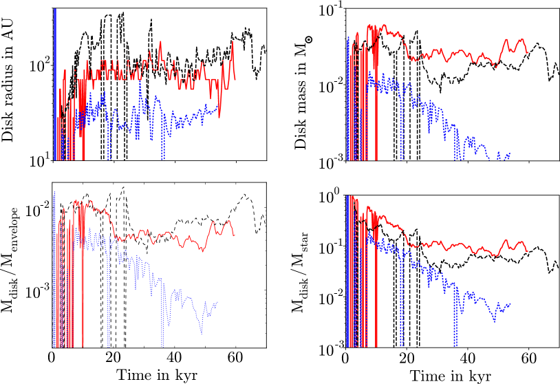
Figure 1: Disc radius (upper left panel), disc mass (upper right panel), ratio of disc and envelope mass $\frac{M_{\rm disc}}{M_{\rm env}}$ (lower left panel) and ratio of disc and stellar mass (lower right panel) around sink b (red solid line), sink d (black dashed line) and sink f (blue dotted line). The disc radius is estimated as the distance from the host sink, where the rotational velocity is less than 80 % of the Kepler speed $v_{K}=\sqrt{\frac{GM}{r}}$. The disc mass is determined as the mass that is located within the disc radius and inside a vertical height from the mid-plane computed as the maximum of 8 au and a vertical-height-to-radius ratio of 0.2.

3.1 Accretion profiles

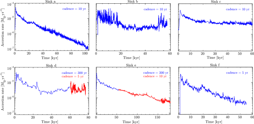
Figure 2: Accretion rate in M_☉yr^-1 for the different sinks as based on the runs carried out with a minimum cell size of 2 au. The cadences for the individual sinks are given in the legend.

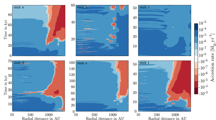
Figure 3: Mass change in solar masses per yr for the mass enclosed within spheres of different radii. The results are based on the runs carried out with a minimum cell size of 2 au.

In K17, we showed that the accretion profiles of different protostars differ from each other due to the molecular cloud environment of the protostellar systems. In this paper, we investigate the effect of an existing protoplanetary disc in the vicinity of the sinks in more detail. To compare the discs around the different sinks, we defined the radius of the disc in K17 as being equivalent to the radial distance from the sink, where the rotational speed dropped to less than 80 % of the Kepler-speed $v_{K}=\sqrt{GM/r}$. We excluded the inner seven cells (14 au) from the sink to avoid accounting for the low rotational velocities induced by the sink at the centre. We then estimated the disc mass to be the enclosed mass within this radius and inside a vertical height from the mid-plane computed as the maximum of 8 au and a vertical-height-to-radius ratio of 0.2. Although these criteria only give a rough estimate of the disc radius and mass, we found clear differences for the different sinks. Around two sinks (sink b and d), discs of several tens of au are formed within a few kyr and evolve to large disc-to-stellar mass ratios $\left(\frac{M_{\rm disc}}{M_{\rm star}}\right)$ of about 10 % at 50 kyr after sink formation. Another sink (sink f) also showed signs of a stable, but smaller and lighter disc (only a few tens of au and $\frac{M_{\rm disc}}{M_{\rm star}}$ of only 1 % at about 50 kyr after sink formation), whereas the vicinity of the remaining sinks either showed no or only weak and intermittent signs of a disc. In Table 1, we briefly summarize the main result of the disc study carried out in K17 by distinguishing between no disc, a weak disc or a massive disc, and in the upper panels of Fig. 1 we show the disc radius (left) and disc mass (right) around sink b, d and f. Moreover, we show in the lower panels of Fig. 1 the ratio between disc mass and envelope mass (left) as well as the ratio between disc mass and sink mass (right). In principle the envelope mass is all the mass that is gravitationally bound inside the collapsing core. As shown in K17, the pre-stellar cores in our simulations are not perfectly symmetric spheres due to the underlying turbulence and the cores are shaped differently. However, as a proxy we simply define the envelope mass as all the mass that is located within 8000 au from the central sink except for the sink mass itself. We find that the three sinks have envelope masses of a few to about 10 M_⊙. Comparing the evolution of the disc mass with the evolution of $M_{\rm disc}/M_{\rm envelope}$ does not indicate a simple correlation between envelope and disc mass. The disc mass around sink b tends to be larger than the disc mass around sink d, but the ratio of $M_{\rm disc}/M_{\rm envelope}$ is generally lower during the evolution. Hence, the plot reveals that sink b has the most massive environment.

3.2 Accretion profiles of the six sinks

In Fig. 2 we show the accretion profiles of the six sinks in our zoom-simulations. Except for the first 60 kyr around sink d and approximately the first 55 kyr around sink e, we trace the accretion of mass on to the sink with higher cadence in time (with 5 or 10 yr instead of 200 or 400 yr as in K17), and thus, we are able to resolve accretion bursts of shorter duration. The cases with the most massive discs – sink b and sink d (sink 4 and sink 6 in our previous study) – show the strongest fluctuations (of more than a factor of 5) in the accretion profile compared to sinks without discs or with only weak discs. The accretion profiles of sink b show fluctuations in the accretion profile of more than a factor of 10 within time intervals of less than 100 yr. In particular, sink b accretes mass intermittently. The sink shows violent phases with strong fluctuations in the accretion rate, and calmer periods with modest fluctuations, both lasting for several to tens of kyr. In comparison to previous studies explicitly studying episodic accretion in more idealized setups without magnetic fields (e.g Vorobyov, 2010, 2011; Stamatellos et al., 2011) , the occurrence of episodic events is lower in our cases. Considering that magnetic fields limit the growth of disks due to magnetic braking, as well as they provide additional pressure support against fragmentation these differences are expected.

In addition to the accretion profile on to the central sink, we are interested in the mass evolution at different distances from the central star. We computed the change in total mass enclosed in spheres (including all the mass that has fallen on to the central sink) of radius $r$ during time intervals of 200 or 400 yr. In Fig. 3 we show the corresponding result in the range of 10–8000 au. As expected, the mass accretion profiles for the innermost radii are similar to the accretion profiles of the sinks. For the cases without discs (sinks a, c, and e), we continuously see mass increase throughout the entire period of the simulation within distances of about 1000 au. However, for the sinks with surrounding discs (sinks b, d, and f), we see brief periods in which the mass enclosed in spheres of a few tens to about several 100 au occasionally decreases. The intermittent decrease of enclosed gas at these scales is caused by temporary outward motion of the gas. Finally, we find that the mass accretion on scales beyond 1000 au differs significantly in the six systems, and is fundamentally shaped by the molecular cloud environment. After an initial increase in total enclosed mass during the first several kyr after sink formation, the total enclosed mass around sinks a, d, e and f decreases with a rate of up to $10^{-4}$ M_☉yr^-1 for spheres with radii larger than $\approx$1000 au. The early total mass increase within small radii traces the collapse of the prestellar core and the subsequent infall of gas from the envelope on to the star–disc system during the first 10 to 20 kyr after the birth of the protostar. In contrast, the total mass evolution within spheres with radii larger than the size of the prestellar core can only increase if additional mass is delivered. The change in mass for spheres with radii larger than $\sim$1000 au trace the motion of the star–disc system through the GMC to regions of different densities. In the cases of sink a, d, e and f, the star–disc system moves to a lower density region, as indicated by the mass decrease at large radii, whereas for sinks b and c, the systems are embedded in regions of higher density. We caution that although the overall mass enclosed within a sphere of several 1000 au in radius may decrease temporarily, the protostellar system may still be fed with additional mass from larger distances.

In K17 we showed that the stars are located in different environments. The system around sink b is embedded in a turbulent environment and 3D visualizations with the tool vapor (Clyne & Rast, 2005; Clyne et al., 2007) show that additional mass approaches the star–disc system. Moreover, a massive clump forms at a distance of about 1500 au from sink b that leads to the formation of a companion about 35 kyr after the formation of sink b. The formation of the companion reflects that sink b is embedded in a dense environment as shown in the column density plot for sink b in Fig. 4. While it is very interesting to catch the formation and evolution of a wide binary system from realistic GMC conditions in a model with high enough resolution to capture au-scale structures like the circumstellar disc, a detailed analysis is beyond the scope of this paper. We will analyse the properties and dynamics of this system in detail in a follow-up paper.

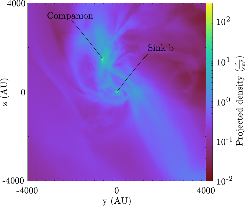
Figure 4: The formation of a wide binary. Column density in the $yz$-plane of the coordinate system with a column height in the $x$-direction of $\pm 8000$ au at $t=35$ kyr after the formation of sink b. Sink b is located at the centre and the companion forms inside the massive clump locate at a relative position of $(x,y,z)\approx(-350,-600,1250)$ au.

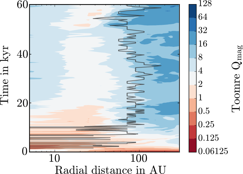
Figure 5: Azimuthally averaged magnetic Toomre parameter $Q_{\rm mag}$ around sink b during disc evolution. The colour bar indicates the strength of $Q_{\rm mag}$ and the solid grey line marks the size of the disc estimated as the radius, where the rotational speed drops to less than 80 % of the Kepler speed $v_{K}=\sqrt{\frac{GM}{R}}$.

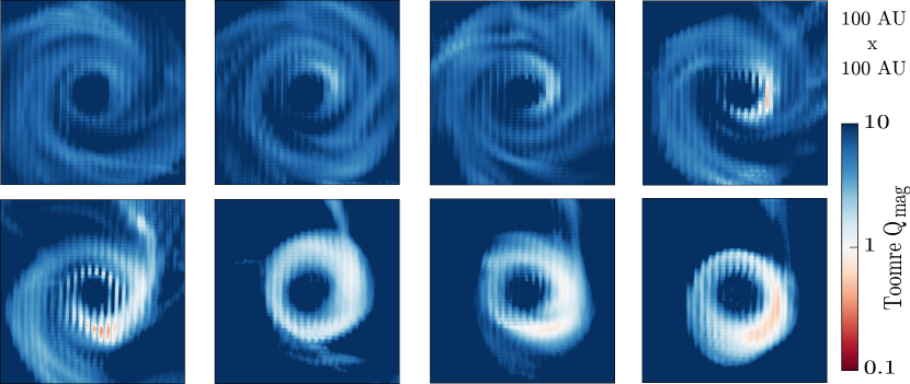
Figure 6: A $100\,\mathrm{au}\times 100\,\mathrm{au}$ image of the magnetic Toomre parameter $Q_{\rm mag}$ around sink b in the disc at $t=49.6$ kyr, $t=50$ kyr, $50.4$ kyr, $t=50.8$ kyr, $51.2$ kyr, $51.6$ kyr, $52$ kyr and $52.4$ kyr. The colour bar indicates the strength of $Q_{\rm mag}$.

3.3 Disc instabilities

3.3.1 Low resolution run with minimum cell size of 2 au

To better understand the influence of the disc on the accretion process, we investigate the stability of the disc around sink b in more detail. Generally, if the ratio of the disc to stellar mass is high enough, it can exceed the support provided by thermal and magnetic pressure, and thus, the disc may become gravitationally unstable. The stability parameter for a magnetized disc is the magnetic Toomre parameter (Toomre, 1964; Kim & Ostriker, 2001)

$$Q_{\rm mag}=\frac{\sqrt{(c_{s}^{2}+v_{A}^{2})}\Omega}{\pi G\Sigma},$$ (4)

with sound speed $c_{s}$, Alfvén speed $v_{A}$, Keplerian orbital angular velocity $\Omega$, gravitational constant $G$ and surface density $\Sigma$. The disc is gravitationally unstable if $Q_{\rm mag}\lesssim 1$. For detailed analyses of the critical number relevant for collapse in non-magnetized local disc simulations addressing the gravitational instability, please refer to Balbus & Papaloizou (1999); Kratter & Murray-Clay (2011); Baehr & Klahr (2015).

Figure 7: Accretion rate for the high-resolution run (black line) and the low resolution run (blue) around sink b based on the same cadence of 10 yr for comparison. The thin green line shows the accretion rate for the high-resolution run at the higher cadence of the underlying data of 1 yr.

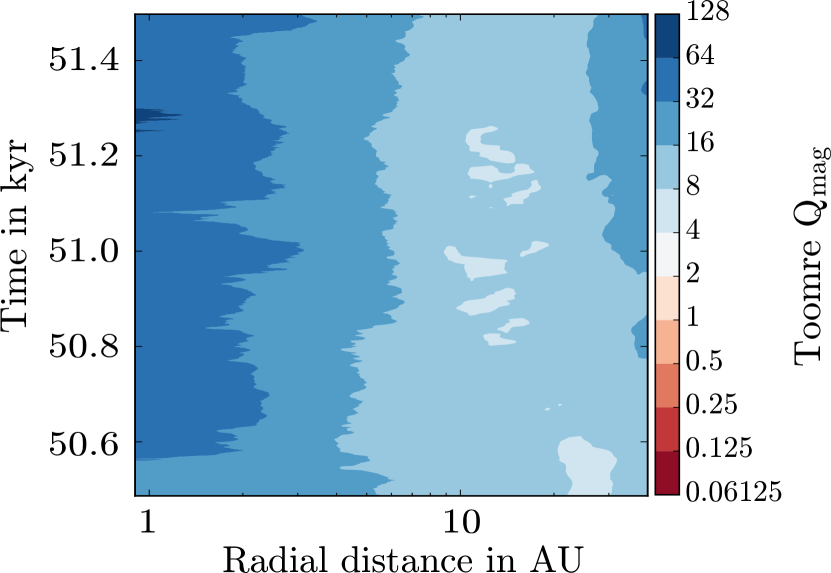
Figure 8: Azimuthally averaged magnetic Toomre parameter $Q_{\rm mag}$ around sink b for the high-resolution run with minimum cell size of 0.06 au for a period of 1 kyr around 51 kyr after sink formation. The colour bar indicates the strength of $Q_{\rm mag}$.

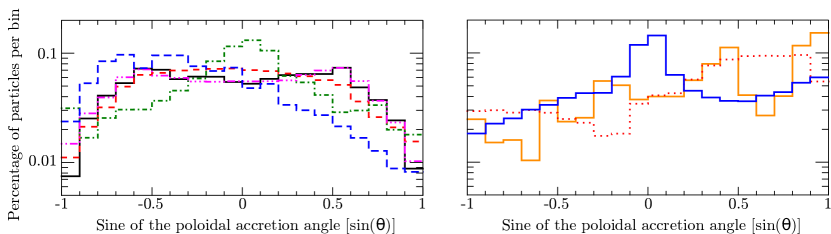
Figure 9: Left-hand panel: Probability distribution of the accretion angle for the different sinks a: black solid line, c: red dashed line, d: green dashed-dotted line, e: magenta dashed-double-dotted line, f: blue long-dashed line). Right-hand panel: Probability distribution for sink b (blue solid line) and the 1 kyr interval shortly after 50 kyr in the 2 au resolution run (orange solid line) and the high-resolution run (red dotted line).

In Fig. 5, we show a space–time diagram of the azimuthally averaged magnetic Toomre parameter based on cylindrical shells of $100$ au in height. The figure shows azimuthal averages that indicate occasionally gravitationally instabilities at some locations in the disc. Comparing Fig. 5 with the accretion profile of sink b (upper middle panel in Fig. 2, we find that the occurrence of low $Q_{\rm mag}$ (i.e. potential gravitational instabilities) correlate with periods of high-accretion rates. This is expected, since angular momentum transport in an unstable disc is efficient. During the first $\sim 20$ kyr, the system is generally unstable or marginally stable with $Q_{\rm mag}<2$, and the accretion rate shows a fluctuating profile with strong bursts. These results are consistent with the evolution of the Toomre parameter around sink d as discussed in K17. While indicative, the Toomre parameter is ill-defined, when no disc is present, and low $Q_{\rm mag}$-values in the early collapse phase should not be over-interpreted. From about 20 kyr to 50 kyr, $Q_{\rm mag}$ is above 2, and the accretion profile is comparatively steady during this period. Between $t=50$ and $60$ kyr, $Q_{\rm mag}$ decreases below 2 at a distance of 20 au, and the sink undergoes a phase of more violent accretion for several thousand yr.

To investigate the spatial distribution of $Q_{\rm mag}$ in more detail, we show the distribution in slices of 100 au $\times$ 100 au of the disc for eight snapshots with 400 yr difference in between $t=49.6$ and $52.4$ kyr in Fig. 6. As anticipated from the azimuthally averaged $Q_{\rm mag}$ profile and from the accretion profile, we find that $Q_{\rm mag}$ locally becomes less than 1 at distances of 10 – 20 au from the sink after $50.8$ kyr. The rapid short-term fluctuations detected in the accretion profiles indeed correlate with the occurrence of gravitational instabilities in the disc as suggested by Stamatellos et al. (2011, 2012); Dunham & Vorobyov (2012); Vorobyov & Basu (2015). However, in our study the instabilities trigger spiral structures in the disc, but fragmentation does not occur. This may be because the areas where $Q_{\rm mag}<1$ are very localized. The mass accretion rate within a spherical distance of several 100 au increases from $10^{-6}$ to $10^{-5}$ M_☉ yr^-1 briefly before and during the burst period, and the disc instability is therefore triggered by infall on to the star–disc system. This scenario is different from the occurrence of an instability in a smooth disc of constant mass.

Figure 10: Illustration of gas falling vertically on to the disc at a radius of $\sim 1$ au at $t=50.515$ kyr based on the high-resolution run with a minimum cell size of $0.06$ au. The image was rendered with vapor and the visible disc is about 10 au in radius. We chose a non-linear density dependent opacity such that low densities are more or even fully transparent, and the disc structure is as apparent as possible. Therefore, the outer parts of the disc are not visible. The red circles/ellipses illustrate the location of the blob at different times and the time cadence between the images is 5 yr.

3.3.2 high-resolution run with minimum cell size of 0.06 au

To gain further insight into the accretion process and to test the robustness of the instabilities in the disc around sink b, we reran a sequence around 51 kyr with higher resolution (minimum cell size 0.06 au, 27 levels of refinement) for 1 kyr. Similar to the zoom-in process before sink formation, we gradually increased refinement level-by-level to continuously allow the cells to adopt to the higher resolution, hence the discrepancy of the accretion profile shortly after $50.5$ kyr. The overall accretion rates are similar to the ones in the lower resolution run (Fig. 7). However, the accretion profile is more flat than in the lower resolution case. This is because the disc is stable against gravitational instabilities with generally higher azimuthally averaged magnetic Toomre parameters of at least $Q_{\rm mag}=4$ during the high zoom-in run as shown in Fig. 8. Therefore, the accretion bursts induced by the gravitational instabilities in the 2 au resolution run are absent in the run with minimum cell size of $0.06$ au. In fact, the higher resolution run shows a smooth, radially decreasing density profile, while in the lower resolution run the infalling mass cannot be transported properly to the inner disc due to the lacking resolution. As a consequence, mass piles up in the disc just outside the accretion region of a few cells (i.e. $\sim$10 au) and builds an artificial mass buffer, which eventually causes gravitational instabilities in the disc. We point out that the cumulative mass at $r\gtrsim 20$ au agree very well in both the low and high-resolution run showing the overall consistency in our runs.

3.4 Angular distribution of the accretion flow

When matter is accreted from the disc or the envelope on to the star potential energy is transferred into kinetic energy, and the kinetic energy is either released as heat at the accretion shock or stored in the rotational energy of the star. This can happen through magneto-spheric accretion channels, which funnels matter from the disc to the star, or in a boundary layer on top of the protostar. How much of the associated accretion luminosity is absorbed by the star and how much is radiated away remains an open question and probably depends on the conditions of the shock front and the geometry of the accretion flow. In the case of a spherical and opaque accretion flow, the star would heat up because it cannot re-emit the radiation in any direction. However, stars may accrete their mass through accretion channels covering only a fraction of the surface. If the region outside the accretion channels is optically thin, the star can efficiently irradiate its accretion energy in the non-accreting directions. We already showed in K17 and in agreement with Seifried et al. (2013, 2015) that mass accretion is filamentary – except for the early collapse phase lasting for a few kyr.

We further constrain the direction from which the mass accretes on to the star. In Fig. 9, we illustrate the probability distribution of the accretion angles as based on the location of tracer particles before they accrete on to the six sinks. On top of that we show the angle distribution obtained from the higher resolution run for sink b and the corresponding distribution for that interval as based on the standard resolution run. We find that the sinks with the strongest discs (sinks b and d) predominantly accrete mass at a small or zero angle with respect to the disc (enhancement at $\sin(\theta)=0$), showing that mass indeed accretes on to the star preferentially from the disc. Generally, we can see for the remaining sinks that mass accretes less likely from the poles as seen in the decrease of the profiles around $\sin(\theta)=\pm 1$. In the cases of sinks a, c, d, and e the angle distribution is approximately symmetric, while for sink b and particularly for sink f the distribution shows that gas predominantly accretes from one side rather than the other. As mentioned above, gas accretion is mostly filamentary and occurs through accretion channels. Using 3D visualization we have validated this, and that gas falls predominantly on to the central region in a plane that is not aligned with the star–disc system during this period, explaining the asymmetry in the angle distribution. When looking at the short interval that was run with higher resolution around sink b, the asymmetry found in the low resolution run persists. We show in Fig. 10 the vertical infall of gas on to the inner part of a young disc at $t\approx 50$ kyr based on the high-resolution run. Gas approaches the disc, forms a gas blob and accretes on to the disc at a radius of $\sim 1$ au. Similar events occur preferentially from one side as a consequence of mass infall explaining the asymmetry in the polar angle during the interval. Besides the asymmetric infall, Fig. 10 illustrates the underlying density structure inside the disc and its evolution during a few to several orbital times of the inner disc. The images demonstrate the importance of accounting for the environment by using global models when studying young discs.

3.5 Effect of episodic accretion on protostellar evolution

Accretion bursts can have a profound impact on the protostellar evolution. When the rate of mass accretion suddenly increases, a much larger fraction – maybe all – of the stellar surface is covered with accreting material (Kley & Lin, 1996). This inhibits the effective radiation and cooling of material before it is added to the star. A significant influx of heat together with new material disrupts the local equilibria that dominate the stellar dynamics (Geroux et al., 2016; Jensen & Haugbølle, 2018). In this section we describe the effects of episodic accretion on the stellar evolution.

Figure 11 shows the evolution of the protostellar radius, effective temperature and various luminosity components during the accretion phase. We start by focusing on the evolution of sink a, sink e, and sink f, which do not feature accretion events with $\dot{M}>10^{-5}\,\mathrm{M}_{\sun}\,\,\mathrm{yr}^{-1}$ of any significance at later times. During the first 10 kyr the protostars undergo a rapid expansion phase caused by the deposition of accretion energy in the outer layers. Due to the dynamical $\alpha(\dot{\mathrm{M}})$ model these high initial accretion rates lead to a high thermal efficiency with $\alpha\approx 0.5$. In combination with a small initial radius and high-accretion rates this gives a relatively high $L_{\mathrm{acc}}^{\mathrm{in}}$ compared to protostellar luminosity $L_{*}$. During this period the thermal energy of the accreted material heats the surface layers of the protostars faster than the energy can be radiated away, which causes a readjustment of the hydrostatic structure. For a comprehensive description of the conditions behind this mechanism we refer to Hartmann et al. (1997). This self-regulating mechanism of the initial protostellar structure for hot accretion models removes the dependence on the initial radius of the model, but introduces a new dependence, namely the efficiency parameter $\alpha$ and the accretion rate (Hosokawa et al., 2011). The expansion is halted as the increased radius of the protostars causes the protostellar luminosity to rise and counterbalance the heat influx from the accreted gas. As the main accretion phase ends the protostar begins an almost steady contraction. At the beginning the stars are still not in a stable hydrostatic configuration, and keep increasing the effective temperature, while eventually around $\sim$100 kyr they start to descend the Hayashi track and evolve similar to that of a classical pre-main-sequence model. It is also around this time the protostars ignite deuterium in the interior.

Next we turn our attention to the evolution of sink b, which is dominated by a number of intense accretion burst. The initial behaviour of the model is similar to that of sink a with a rapid readjustment of the hydrostatic equilibrium. After this initial phase we see a number of accretion events with $\dot{M}>10^{-5}\,\mathrm{M}_{\sun}\,\,\mathrm{yr}^{-1}$. Each of them are followed by an increase in radius and effective temperature, which is a consequence of the same mechanism responsible for the initial expansion. Due to the dynamical $\alpha$-model the accretion is hot with $\alpha$ approaching $0.5$ during an accretion event. The hot accretion combined with the high-accretion rates causes a significant rise in $L_{\mathrm{acc}}^{\mathrm{in}}$, which heats the outer layers of the protostar and prompts a readjustment of the stellar structure. This behaviour during accretion events with hot accretion is in agreement with the results of Baraffe et al. (2012), who also studied the effects of accretion burst on accreting protostars. After the accretion event the protostar quickly contracts and settles down to the previous configuration. The accretion event pauses the contraction of the protostar, and delays the approach to the main sequence, however the effective delay is small compared to the overall timescale of star formation. The effects of episodic accretion on the timescales of star formation is analysed in detail by Jensen & Haugbølle (2018).

The stellar expansion and rise in effective temperature leads to a higher stellar luminosity, which, combined with the rise in outward accretion luminosity during such a burst, can lead to significant changes in the total luminosity of the protostar.

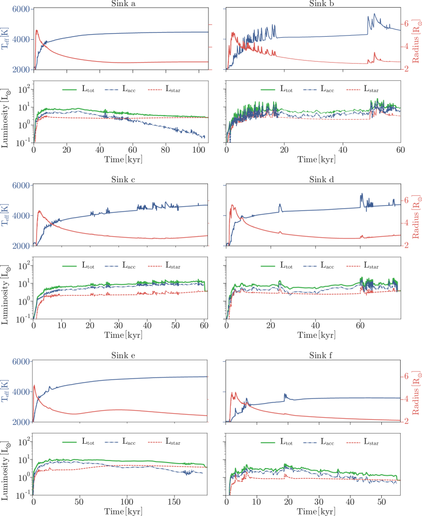
Figure 11: Stellar properties computed with mesa based on the accretion profiles of the six sinks shown in Fig. 2. Panels in rows 1, 3, and 5: Evolution of effective temperature (blue colour) and radius (red colour) of the protostar; Panels in rows 2, 4, and 6: Evolution of the stellar (red dashed), accretion (blue dashed–dotted) and total (green solid) luminosity.

3.6 Observational signatures of episodic accretion in the dust continuum

An accretion burst is expected to manifest itself by increased continuum emission at all wavelengths with a response time of days or hours at infrared wavelengths, and a response time of up to a few months at sub-mm wavelengths (Johnstone et al., 2013). Given that classical FUor outbursts are generally expected to have durations >10 yr the timescale is short enough that it will be possible to directly detect the increased luminosity due to an accretion burst, even in deeply embedded objects that can only be detected at long wavelengths.

Here, we study the variation in the continuum emission in the sink b system, which shows the most accretion variability. We focus on the 1 kyr stretch of the simulation that was rerun with 27 levels of refinement corresponding to a minimum cell size of 0.06 au. As discussed in section 3.3 the accretion profiles differ between the low- and high-resolution runs because of more efficient angular momentum transport in the high-resolution disc. Fig. 12 shows the total luminosity (intrinsic luminosity plus accretion luminosity) of sink b for the two available resolutions. The 2 au resolution run shows a regular long-lived accretion burst, while the 0.06 au resolution run also shows a high degree of variability, but the bursts are weaker and have shorter duration relative to the 2 au resolution case.

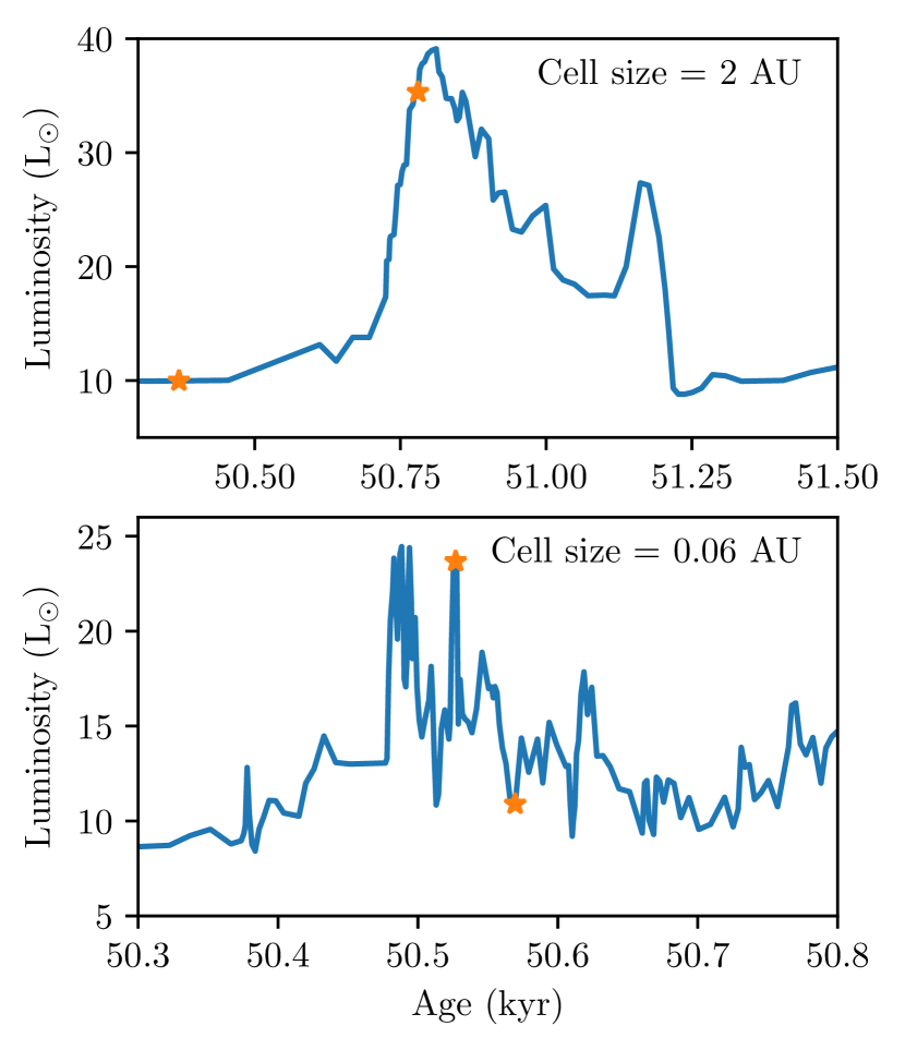
Figure 12: Total luminosity (accretion plus intrinsic) of sink b for both the 2 au resolution case (top) and 0.06 au resolution (bottom). The stars on the curves represent the snapshots where the radiative transfer models were calculated.

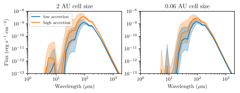
Figure 13: Low and high-accretion rate SEDs for both the 2 au resolution case (left) and the 0.06 au resolution (right). In each case the SEDs have been calculated along 12 different projection directions corresponding to the 12 vertices of an icosahedron to ensure a uniform distribution over the $4\pi$ solid angle. The solid line show the mean flux in each wavelength bin, while the shaded region gives the 1$\sigma$ uncertainty region.

Table 2: Synthetic observables

Model	Age	$L_{\mathrm{input}}$	$L_{\mathrm{bol}}$	$T_{\mathrm{bol}}$	$L_{\mathrm{smm}}/L_{\mathrm{bol}}$
	(kyr)	(L☉)	(L☉)	(K)	(%)
2 au low accretion	50.4	10.0	$8.7\pm 3.5$	$42\pm 8$	$1.3\pm 0.7$
2 au high-accretion	50.8	35.3	$27.7\pm 16.5$	$48\pm 13$	$0.8\pm 0.5$
0.06 au high-accretion	50.5	23.7	$21.2\pm 10.1$	$46\pm 10$	$0.9\pm 0.5$
0.06 au low accretion	50.6	10.9	$9.7\pm 3.8$	$41\pm 8$	$1.3\pm 0.7$

We calculate radiative transfer models for four different snapshots; two for each available resolution with one model corresponding to a low accretion rate and the other to a high-accretion rate. Figure 13 shows the SEDs calculated for the four radiative transfer models, while Table 2 lists some basic quantities calculated from the SEDs. As described in Section 2.3 the synthetic SEDs are calculated along 12 different lines of sight distributed evenly over the $4\pi$ solid angle, and the quantities listed in Table 2 are the average and 1sigma standard deviations calculated from the individual SEDs.

As can be seen from Table 2 the average bolometric luminosity inferred by integrating over the SEDs is always somewhat smaller than the input luminosity; something that can be attributed to the limited size of the aperture, which means that some fraction of the emission from the system remains uncovered. Also, the uncertainty on the bolometric luminosity is quite large, which indicates that the inferred luminosity depend strongly on the line-of-sight. This is a well-known issue for systems that contain a disc, where shielding in the disc plane can easily attenuate the emission from the central by a factor of 2 (e.g. Whitney et al. 2003; Frimann et al. 2016). The situation is further aggravated in the situation at hand since the system is traversed by a massive filament running roughly perpendicular to the disc, meaning that many lines of sight close to face-on to the disc are also subject to high column densities.

Table 2 also shows the bolometric temperature, $T_{\mathrm{bol}}$ (Myers & Ladd, 1993) and the ratio between the sub-millimetre luminosity (the integral of the SED over wavelengths > 350 $\mu$m) and bolometric luminosity, $L_{\mathrm{smm}}/L_{\mathrm{bol}}$ (André et al., 1993), both of which are commonly used tracers of the evolutionary stage of the protostar. The low value of $T_{\mathrm{bol}}$ (<70 K) and high value of $L_{\mathrm{smm}}/L_{\mathrm{bol}}$ (>0.5 %) shows that observationally the protostellar system would be consistent with being a deeply embedded Class 0 source. The embedded nature of the source can also be appreciated by looking at the SEDs in Fig. 13. The emission is hardly detected at wavelengths <10 $\mu$m, and the width of the shaded regions show that projection effects play an important role indicating that the dust is optically thick. At wavelengths $\gtrsim$100 $\mu$m when the dust becomes optically thin the emission from the SED becomes independent of the line-of-sight.

For the 2 au resolution case the input luminosity increases from 10.0 to 35.3 $L_{\odot}$ between the two snapshots corresponding to a fractional increase of a factor 3.5. We can also estimate the observed fractional increase by integrating over the SEDs and calculating the ratio for each of the 12 lines of sight. Doing this yields a fractional luminosity increase of 3.1 $\pm$ 0.4 $L_{\odot}$. For the 0.06 au resolution case the fractional increase in the input luminosity is somewhat smaller at a factor of 2.2, while the observed fractional increase is 1.9 $\pm$ 0.4 $L_{\odot}$. Looking at the SEDs in Fig. 13, we see that high-accretion SEDs have systematically greater fluxes relative to the low accretion SEDs for wavelengths $\gtrsim$ 20 $\mu$m. Below 20 $\mu$m the SEDs are dominated by noise because of the extremely high optical depths inherent to embedded protostars. The fractional flux increase is not uniform over the SED but is greater at shorter wavelengths, and consequently bursts will be easiest to detect at the shortest wavelength where the source can be detected. For the 2 au resolution case the fractional increase of the flux at 25, 70, 100, and 1000 $\mu$m is 7.4, 4.1, 2.8, and 1.4. For the 0.06 au resolution case the fractional increases at the same wavelengths are 5.5, 2.6, 2.0, and 1.2.

The fractional luminosity increases studied here are smaller than classical FUor outburst, which typically increase their luminosities by a factor of 10 or more. However, the fractional luminosity increases is significantly above the typical variability observed in young stars, which is typically below 20% at mid-infrared wavelengths (e.g. Rebull et al. 2015; Flaherty et al. 2016; Rigon et al. 2017).

4 Discussion

4.1 Implications of late infall

The intermittently high-accretion rate at late times for sink b harboured in a high-density environment indicate that star–disc systems can be fed by gas that initially was more than $10^{4}$ au away from the star at the time of stellar birth. Our small sample does not allow for a statistical study of the frequency of these late infall events. However, the weaker signs for another case (sink 8 in K17, not discussed in this work) as well as significant mass increase of several sinks after $t>100$ kyr in our parental run indicates that such infall is common. As also discussed by Padoan et al. (2014), we suggest that late infall events is an important part of the solution to the luminosity problem encountered for YSOs. Late infall may be the reason for recent observations of misaligned outer and inner discs (Brinch et al., 2016; Benisty et al., 2017). In the case of the binary system IRS 43, Brinch et al. (2016) found that the circumbinary disc has a different orientation than the orbital plane of the binary, as well as their corresponding discs. Benisty et al. (2017) find a misalignment of 72 degrees between the inner and outer disc around HD 100453. Considering the underlying turbulent motions in the molecular cloud, gas that falls on to the system at later times is likely to have a different angular momentum than the net angular momentum of the star–disc system at the time of the infall. If the rotational component is strong enough, the system may well establish an outer misaligned disc. Moreover, infall of material with different angular momentum may also lead to changes of the disc properties such as the disc size and disc mass (Vorobyov et al., 2015).

Furthermore, late infall may have profound consequences for the formation of planets. Typical disc lifetimes of about 1 to a few Myr (Haisch et al., 2001; Mamajek, 2009) and the observations of gap and ring structures in young discs (e.g. ALMA Partnership et al., 2015) indicate that planet formation starts early after star formation. Potentially, late infall can thus also enrich the mass reservoir in the disc at times during planet formation. While outside the scope of the current paper, we plan to continue the simulations, in particular the ones for the more embedded sinks (sinks b and d), to constrain the potential importance of late infall at times much later than 100 kyr.

While it is certainly possible that fragments landing directly on the stellar surface could be part of the solution, our results suggest a scenario of infall and disc instabilities as the explanation for episodic accretion. The current selection of zoom-in runs were chosen to be in relatively quiet areas of the star-forming region. Looking at the selection of solar mass stars in Jensen & Haugbølle (2018) much more violent infall rates are possible. There are also indications (Frimann et al., 2017) that episodic accretion may be linked with binary systems.

4.2 Limitations in the zoom-simulations

Carrying out deep AMR simulations covering all scales from a GMC down to protoplanetary disc scales is technically challenging and computationally expensive, even if done for a single star. We have made many changes compared to the public version of ramses, which collectively have increased both the single core performance and the scalability of the code. Nonetheless, we cannot currently afford to include all physical processes potentially relevant in protoplanetary discs to full extent, nor can we apply arbitrary high-resolution for simulating several thousand yr of disc formation and evolution yet. Recent developments of new codes (e.g. athena++) or code frameworks such as dispatch (Nordlund et al., 2017) will help to overcome some of these limitations.

Magnetic fields are a crucial component in star formation, and we account for the magnetic fields present in GMCs during the formation and evolution of protoplanetary discs consistently. Together with the underlying differences in the morphology of the gaseous filaments in the cloud, we are thus able to naturally explore different conditions for star and protoplanetary disc formation. However, we assume the gas to be perfectly coupled to the magnetic fields and use ideal MHD in our simulations. It is well known that the gas in protostellar systems is far from being perfectly coupled, due to very low degrees of ionizations, and non-ideal MHD effects such as Ohmic dissipation, ambipolar diffusion, or the Hall effect can become important during the formation (e.g. Machida et al., 2008; Joos et al., 2012; Joos et al., 2013; Li et al., 2011; Wurster et al., 2016; Hennebelle et al., 2016; Masson et al., 2016) and evolution of stars and protoplanetary discs (e.g. Gressel et al., 2015; Béthune et al., 2017; Bai & Stone, 2017). These effects would generally cause a decreasing magnetic field strength, and we most likely overestimate the effects of magnetic braking, as well as the strength of magnetic fields inside our discs. As discussed in K17, we expect to underestimate the presence, size and mass of the discs in our simulations partly because of the ideal MHD approach. Considering the potential overestimate of the magnetic field strength, the magnetic field further prevents gravitational instabilities inside the discs in our simulations. It is beyond the scope of this work to study the details of the magnetic field structure. We refer the reader to Kuffmeier & Nauman (2017), in which we investigate the strength and topology of magnetic fields in discs inherited from and anchored in the fields penetrating the GMC.

The other relevant pressure component in our disc is thermal pressure. Tsukamoto et al. (2015) demonstrated that radiation transfer causes heat-up of the disk even in its outer parts. We have not included radiative transfer (e.g. by using the ray-tracing scheme implemented in the Copenhagen version of ramses Bisbas et al., 2015), and since our table based cooling implementation assumes radiatively thin cooling above a temperature floor of 10 K, our discs are generally colder than they would be in reality. A hotter disc would be more stable, with an additional thermal pressure, suppressing the occurrence of gravitational instabilities in the disc, in contrast to the effect of a lower magnetic field. Furthermore, the infall of clumps on to the star–disc system causes a local heat-up inside the disc. In principle, if the heat-up is efficient enough, it may hinder the onset of a gravitational instability in the disc. In reality however, we expect the heating to be not so drastic since mass accretion scales to the temperature as $\dot{M}\propto T^{4}$. Moreover, gravitational instability in the disc may occur for short cooling times, whereas longer cooling times suppress it (Gammie, 2001; Lodato & Rice, 2004; Mejía et al., 2005; Meru & Bate, 2012; Paardekooper, 2012; Baehr & Klahr, 2015).

The accretion rates in the low and the high-resolution models of sink b are on average consistent though the presence of gravitational instabilities in the low resolution run induces bursts lasting for $\sim 100$ yr. As explained above the gravitational instabilities in the low resolution run at this time are induced by a mass buffering effect. In the high-resolution run we resolve the inner parts of the disc, which circumvents the pile up of gas at $\approx 10$ au. Therefore, gravitational instabilities are absent in the high-resolution run around $t=50$ kyr, and hence the accretion rate varies less in the high-resolution run than the low resolution run at a cadence of 10 yr. Comparing the accretion profile sampling with a cadence of 10 yr to that sampled with 1 yr, closer to the orbital time at distances < 1 au from the sink particle, we find larger fluctuations in the high-resolution run. In the case of the low resolution run 10 yr correspond to about two orbital times at the resolution of 2 au for the mass of sink b of $m\approx 0.3$ M_⊙ at $t\approx 50$ kyr. Considering the the minimum cell size of $0.06$ au as a radius, 10 yr correspond to more than 365 orbital times. Given that the sink accretes mass mostly from the innermost cells, plotting with a 10 yr cadence we partly average out the resolved fluctuations present in the high-resolution run by using a lower cadence. This can be appreciated in Fig. 7, where the 1 yr cadence is shown by a thin green line.

In Fig. 9, we illustrated the accretion angle of the gas on to the sink. However, at the current limits of resolution we do not capture adequately the real paths taken by gas accreting to the protostellar surface. The protostar itself is magnetized and depending on the accretion rates gas may accrete on to it in funnels at distances much smaller than 1 au in the form of magneto-spheric accretion (Hartmann et al., 1994), or through a magnetized boundary layer. To constrain the thermal efficiency parameter $\alpha$ precisely based on our zoom-simulations is therefore not possible, due to the combination of lacking resolution and microphysics. Nevertheless, the simulations show that gas can accrete on to the star at a range of angles, but if a disc is present the gas preferentially approaches the protostar along the disc mid-plane. The existence of even a small circumstellar disc may therefore be an important factor in regulating the thermal efficiency of the accretion flow.

4.3 Protostellar evolution

We have calculated the protostellar evolution assuming a dynamic model of the thermal efficiency near the accretion shock. The evolution of the protostellar structure depends to some extent on the exact model used (Jensen & Haugbølle, 2018). The radial expansion during the initial main accretion phase and during episodic burst later on depends on the upper limit on $\alpha$. A similar effect is not present for the effective temperature of the protostar, which is much more insensitive to the details of the thermal efficiency $\alpha$. This is partly a result of the way accretion energy is distributed in the model. In our implementation the specific accretion energy is distributed evenly across the outermost radial shells of the protostar as opposed to depositing the entire energy in the outermost shell. We set an upper limit on the specific energy added to each radial shell, which regulates the extent of the region where the energy is deposited. During a burst the accretion energy will therefore be spread out over a larger amount of radial shells rather than resulting in an increased energy injection in the outermost cell. This effect can cause the effective temperature of the protostellar models to be underestimated, but it should not significantly alter the evolution of the protostar, since in any case convection will rapidly redistribute the added heat (Jensen & Haugbølle, 2018).

We expect models with a higher thermal efficiency to have longer contraction times, which delay the onset of deuterium burning as well as the overall evolution of the models (Kunitomo et al., 2017). However, this effect is negligible in our study, where we are mostly interested in significant luminosity enhancements induced by episodic accretion at early times. In principle, an accretion burst, such as those observed for sink b, both changes the luminosity and the effective temperature. It therefore correspond to a diagonal displacement in the Hertzsprung–Russel diagram. This is important for more evolved protostars that are not embedded anymore, where the change in temperature can result in an overestimate of the mass. In the embedded case though changes in the stellar SED is masked, since all radiation is reprocessed by the dust.

4.4 Comparison with observations

OO Serpentis is a Class I protostar in the Serpens NW star-forming region, which was observed to undergo an accretion burst in 1995. Kóspál et al. (2007) found ratios of the peak brightness relative to the preoutburst brightness > 10 at wavelengths 2.2, 12, 25, and 60 $\mu$m. In particular, the fractional increase at 25 $\mu$m was measured to $\approx$25. The detection at wavelengths <10 $\mu$m in OO Serpentis is consistent with OO Serpentis being a Class I object, whereas the synthetic observations point towards the simulated source being a deeply embedded Class 0 object. Probably, the best known direct observation of an accretion burst in a deeply embedded object is the case of HOPS 383, a Class 0 protostar in Orion, which was observed to increase its 24 $\mu$m flux by a factor of 35 between 2004 and 2008 corresponding to an increase in luminosity from $\sim$0.2 to $\sim$7.5 L_☉ (Safron et al., 2015). The fractional increase of the brightness at 24–25 $\mu$m of OO Serpentis and HOPS 383 is significantly larger than the corresponding increase of a factor of 7.4 and 5.5 seen for the 2 au and 0.06 au resolution burst. Recently, Hunter et al. (2017) detected a burst in the massive protocluster NGC 6334I quadrupling its brightness at mm wavelengths corresponding to a fractional increase of its luminosity of $70\pm 20$. We remark that NGC 6334I is not a single object but a massive cluster consisting of $\sim$5 individual sources, and thus the situation may not be completely equivalent to that of a low-mass single protostar like the one studied here.

The simulated bursts discussed in this work are much weaker indicating that such drastic bursts as discussed above are exceptional. Nevertheless, we stress that although the increase in luminosity of the simulated bursts is smaller than the above observations or the order of magnitude increases of a classical FUor type object, they are still significant enough to be observable. For example Scholz et al. (2013) surveyed 4000 YSOs in the Galactic plane over 5 yr and found only four with a fractional flux increase >2.5 at wavelengths of 3.6 $\mu$m, and 4.5 $\mu$m, which is comparable to our simulated bursts. One problem to constrain the frequency of episodic accretion events is the difficulty in determining whether a protostar underwent an accretion burst event in the past. A promising method to circumvent this issue is to look for extended C¹⁸O emission as a signpost of previous accretion bursts (Jørgensen et al., 2015; Frimann et al., 2017).

5 Conclusion

In this work, we investigated the accretion process of six young protostars that are formed in a Giant Molecular Cloud. We followed the stars during up to 180 kyr of evolution after the protostellar birth. By applying adaptive mesh refinement, we are – for the first time – able to follow the formation and evolution of star–disc systems accounting both for gas infall and disc instabilities consistently. The environment around the protostars is determining for the global evolution in the accretion profile, and we find significant variations among the protostars in the overall shape of both their early and late accretion histories. In particular, we find that the presence of a disc increases the frequency of accretion bursts, while the amplitude is related the mass reservoir in the disc. We find that infalling gas acts as the main supplier for the disc and thus for the occurrence of high-accretion rates also at times when the protostar is otherwise already evolved. A detailed analysis of the accretion process shows that mass may accrete on to the sink with a significant angle to the disc midplane. Specifically, a run carried out with higher resolution shows that mass blobs may fall vertically on to the inner part of the disc.

In simulations with a maximum resolution of 2 au, local gravitational instabilities in the disc occur around 20 – 40 au from the sink that correlate with short accretion bursts up to $\sim 10$ higher than prior to the burst on time-scales of about $100$ yr in agreement with previous results by Stamatellos et al. (2011, 2012); Dunham & Vorobyov (2012); Vorobyov & Basu (2015). Follow-up simulations with a maximum resolution of 0.06 au in the vicinity of the sink show similar overall accretion profiles, but lack the existence of gravitational instabilities in the disc, and hence do not show as accentuated accretion bursts as those seen in the lower resolution run, though the intermittency goes up as a result of the shorter orbital time-scale resolved in the high-resolution run. We find that the gravitational instabilities in the low resolution run are induced by a buffering effect probably due to insufficient resolution for the inner disc. Due to the computational difficulty of following the disc evolution with a maximum resolution of 0.06 au for more than 1000 yr, which is a short period compared to the disc lifetime, we do not know if the high-resolution run will evolve similar disc instabilities as the low resolution run at later times.

By looking at the mass evolution around the protostars, we find that for the six sinks we have studied the gas associated with the prestellar core collapses within $\sim$10 kyr to a more compact object with an envelope of $\approx$1000 au in radius. Most of the selected protostars have a relatively uncomplicated accretion history, due to isolated formation sites in the GMC, which from a numerical point of view make them easier to evolve. In a few cases though – sink b being the most prominent – the protostars are located in a more cluster like environment, where the envelope at later times can be fed typically by local high-density filaments. Late infall of gas with an angular momentum orientation different from the initial envelope and the already formed star–disc system may be the explanation for recent observations of systems with misaligned inner and outer discs.

To properly constrain the effects of episodic accretion on the protostellar evolution, we studied the accretion process in more detail by evolving the characteristics of the protostars with the stellar evolution code mesa. We find that the accretion luminosity corresponding to the rapid enhancement of the protostellar accretion rate triggers luminosity bursts. As an additional consequence of such accretion events, the temperature and radius of the protostar increases. To compare directly with observations, we post-processed the simulations with the radiative transfer tool radmc3d  to study the resulting spectral energy distributions of the protostars in detail. In line with previous works, bursts in the accretion rate enhance the flux of the protostar at sub-mm and shorter wavelengths. In particular, we study one burst period in more detail and find enhancements of a factor of about 5 at 24 $\mu$m wavelength Such enhancements at this wavelength, even though lower than the observed increase of a factor of 35 for HOPS 383 (Safron et al., 2015) would be possible to observe.

Appendix A Numerical Convergence

As discussed in the article, some of the most prominent accretion bursts in the accretion profile of the low resolution run of sink b are triggered by gravitational instabilities in the disc. However, these instabilities, and hence the corresponding accretion bursts, happen close to the accretion radius of the sink particle and seem to be induced by a mass buffering effect in the low resolution run. When increasing the resolution, and therefore decreasing the physical size of the accretion radius in the high-resolution run, the effect disappears, and the amplitude of the bursts is decreased by up to a factor of 5. To investigate if this is a common trend, and in order to constrain the numerical convergence of the accretion rates further, we have carried out comparison runs with a maximum resolution of $0.25$ au for sink b, as well as for two other sinks that also maintain a circumstellar disk (sink d and sink f). In all cases we have carried out these tests 50 kyr after star formation over a time interval of about 1000 yr. The accretion profiles are shown in Fig. 14. We find that the $0.25$ au run (black solid line) agrees well with the $0.06$ au resolution run (red dotted line) in the case of sink b, while the $2$ au resolution run clearly differs. The reason for this is that we avoid the artificial mass buffering effect in both the $0.25$ au and the $0.06$ au resolution runs. Nevertheless, all three profiles are in approximate agreement, when integrating for longer time intervals. For the two other sinks, on the other hand, there are no indications of problems. In both cases there is good agreement for the accretion profiles between the 2 au resolution and the $0.25$ au comparison runs. In both cases the higher resolution run has a more intermittent accretion profile, but agrees reasonably well with the lower resolutions runs in a time-averaged sense. Considering that we resolve the inner dynamics of the disk in more detail in the $0.25$ au resolution runs compared to the 2 au resolution run, the lack of such fluctuations in the low resolution run is expected. We may see a tendency towards slightly enhanced accretion rates in the 2 au resolution runs compared to the higher resolution runs with $0.25$ au, but this is at best minor. We conclude that the accretion profiles of the 2 and the $0.25$ au resolution runs are in good agreement for the purpose of this study and accounting for the computational costs involved in running the zoom-ins.

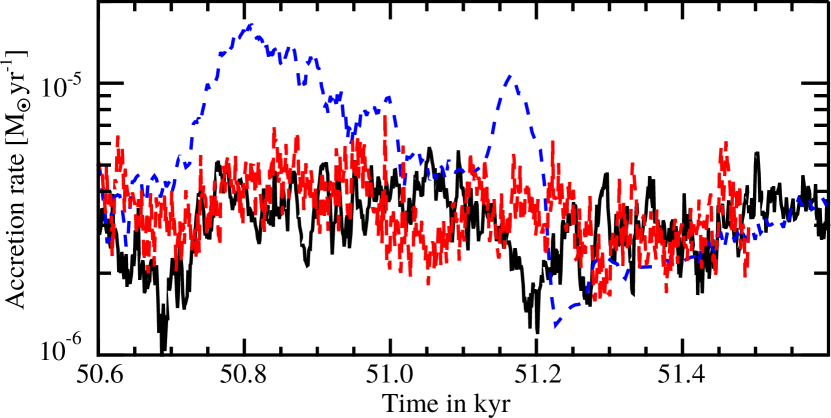
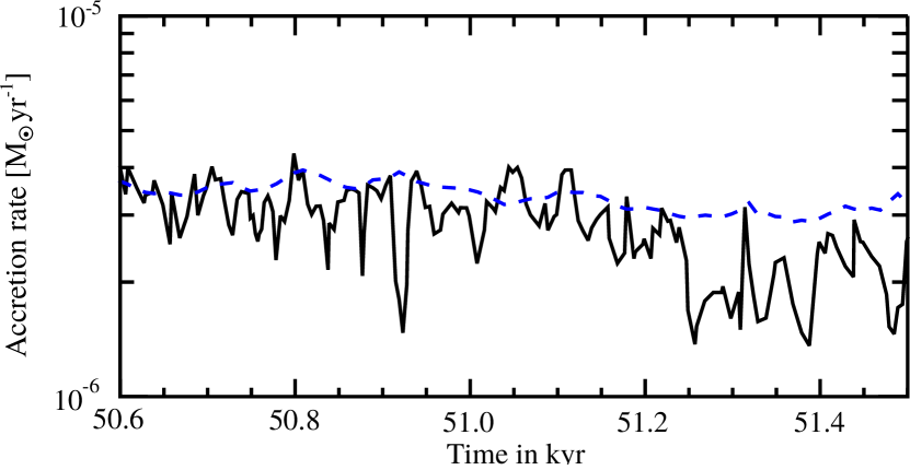
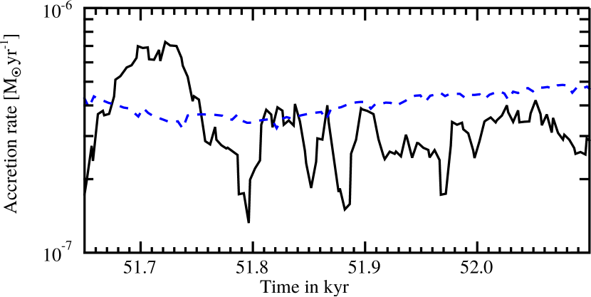
Figure 14: Accretion rates for sink b (top), sink d (middle) and sink f (bottom) of runs with 2 au resolution (blue dashed line) and of runs with $0.25$ au resolution run (black solid line). For sink b, we also plot the accretion profile of the $0.06$ au resolution run (red dotted line).

References

- ALMA Partnership et al. (2015) ALMA Partnership et al., 2015, ApJ, 808, L3
- André et al. (1993) André P., Ward-Thompson D., Barsony M., 1993, ApJ, 406, 122
- Arce et al. (2013) Arce H. G., Mardones D., Corder S. A., Garay G., Noriega-Crespo A., Raga A. C., 2013, ApJ, 774, 39
- Bachiller et al. (1990) Bachiller R., Martin-Pintado J., Tafalla M., Cernicharo J., Lazareff B., 1990, A&A, 231, 174
- Bachiller et al. (1991) Bachiller R., Martin-Pintado J., Planesas P., 1991, A&A, 251, 639
- Baehr & Klahr (2015) Baehr H., Klahr H., 2015, ApJ, 814, 155
- Bai & Stone (2017) Bai X.-N., Stone J. M., 2017, ApJ, 836, 46
- Balbus & Papaloizou (1999) Balbus S. A., Papaloizou J. C. B., 1999, ApJ, 521, 650
- Baraffe et al. (2009) Baraffe I., Chabrier G., Gallardo J., 2009, ApJ, 702, L27
- Baraffe et al. (2012) Baraffe I., Vorobyov E., Chabrier G., 2012, ApJ, 756, 118
- Benisty et al. (2017) Benisty M., et al., 2017, A&A, 597, A42
- Béthune et al. (2017) Béthune W., Lesur G., Ferreira J., 2017, A&A, 600, A75
- Bisbas et al. (2015) Bisbas T. G., et al., 2015, MNRAS, 453, 1324
- Bjorkman & Wood (2001) Bjorkman J. E., Wood K., 2001, ApJ, 554, 615
- Brinch et al. (2016) Brinch C., Jørgensen J. K., Hogerheijde M. R., Nelson R. P., Gressel O., 2016, ApJ, 830, L16
- Choi et al. (2016) Choi J., Dotter A., Conroy C., Cantiello M., Paxton B., Johnson B. D., 2016, ApJ, 823, 102
- Clyne & Rast (2005) Clyne J., Rast M., 2005, in Electronic Imaging 2005. pp 284–294
- Clyne et al. (2007) Clyne J., Mininni P., Norton A., Rast M., 2007, New Journal of Physics, 9, 301
- Dullemond & Dominik (2004) Dullemond C. P., Dominik C., 2004, A&A, 417, 159
- Dunham & Vorobyov (2012) Dunham M. M., Vorobyov E. I., 2012, ApJ, 747, 52
- Dunham et al. (2013) Dunham M. M., et al., 2013, ApJ, 145, 94
- Evans et al. (2009) Evans II N. J., et al., 2009, ApJS, 181, 321
- Ferrière (2001) Ferrière K. M., 2001, Reviews of Modern Physics, 73, 1031
- Flaherty et al. (2016) Flaherty K. M., DeMarchi L., Muzerolle J., Balog Z., Herbst W., Megeath S. T., Furlan E., Gutermuth R. A., 2016, ApJ, 833, 104
- Franco & Cox (1986) Franco J., Cox D. P., 1986, PASP, 98, 1076
- Freedman et al. (2008) Freedman R. S., Marley M. S., Lodders K., 2008, ApJS, 174, 504
- Frimann et al. (2016) Frimann S., Jørgensen J. K., Haugbølle T., 2016, A&A, 587, A59
- Frimann et al. (2017) Frimann S., et al., 2017, A&A, 602, A120
- Gammie (2001) Gammie C. F., 2001, ApJ, 553, 174
- Geroux et al. (2016) Geroux C., et al., 2016, A&A, 588, A85
- Gnedin & Hollon (2012) Gnedin N. Y., Hollon N., 2012, ApJS, 202, 13
- Gressel et al. (2015) Gressel O., Turner N. J., Nelson R. P., McNally C. P., 2015, ApJ, 801, 84
- Grevesse & Sauval (1998) Grevesse N., Sauval A. J., 1998, Space Sci. Rev., 85, 161
- Haisch et al. (2001) Haisch Jr. K. E., Lada E. A., Lada C. J., 2001, ApJ, 553, L153
- Hartmann et al. (1994) Hartmann L., Hewett R., Calvet N., 1994, ApJ, 426, 669
- Hartmann et al. (1997) Hartmann L., Cassen P., Kenyon S. J., 1997, ApJ, 475, 770
- Haugbølle et al. (2017) Haugbølle T., Padoan P., Nordlund A., 2017, ArXiv e-prints, accepted by ApJ,
- Hennebelle et al. (2016) Hennebelle P., Commerçon B., Chabrier G., Marchand P., 2016, ApJ, 830, L8
- Herbig (1966) Herbig G. H., 1966, Vistas in Astron., 8, 109
- Herbig (1977) Herbig G. H., 1977, ApJ, 217, 693
- Herbig (1989) Herbig G. H., 1989, ESO Workshop on Low Mass Star Formation and Pre-Main Sequence Objects, 33, 233
- Hosokawa et al. (2011) Hosokawa T., Offner S. S. R., Krumholz M. R., 2011, ApJ, 738, 140
- Hunter et al. (2017) Hunter T. R., et al., 2017, ApJ, 837, L29
- Inutsuka et al. (2010) Inutsuka S.-i., Machida M. N., Matsumoto T., 2010, ApJ, 718, L58
- Jensen & Haugbølle (2018) Jensen S. S., Haugbølle T., 2018, MNRAS, 474, 1176
- Johnstone et al. (2013) Johnstone D., Hendricks B., Herczeg G. J., Bruderer S., 2013, ApJ, 765, 133
- Joos et al. (2012) Joos M., Hennebelle P., Ciardi A., 2012, A&A, 543, A128
- Joos et al. (2013) Joos M., Hennebelle P., Ciardi A., Fromang S., 2013, A&A, 554, A17
- Jørgensen et al. (2015) Jørgensen J. K., Visser R., Williams J. P., Bergin E. A., 2015, A&A, 579, A23
- Kenyon et al. (1990) Kenyon S. J., Hartmann L. W., Strom K. M., Strom S. E., 1990, AJ, 99, 869
- Kim & Ostriker (2001) Kim W.-T., Ostriker E. C., 2001, ApJ, 559, 70
- Kley & Lin (1996) Kley W., Lin D. N. C., 1996, ApJ, 461, 933
- Kóspál et al. (2007) Kóspál Á., Ábrahám P., Prusti T., Acosta-Pulido J., Hony S., Moór A., Siebenmorgen R., 2007, A&A, 470, 211
- Kratter & Murray-Clay (2011) Kratter K. M., Murray-Clay R. A., 2011, ApJ, 740, 1
- Kryukova et al. (2012) Kryukova E., Megeath S. T., Gutermuth R. A., Pipher J., Allen T. S., Allen L. E., Myers P. C., Muzerolle J., 2012, AJ, 144, 31
- Kuffmeier & Nauman (2017) Kuffmeier M., Nauman F., 2017, preprint, (arXiv:1710.11195)
- Kuffmeier et al. (2016) Kuffmeier M., Frostholm Mogensen T., Haugbølle T., Bizzarro M., Nordlund Å., 2016, ApJ, 826, 22
- Kuffmeier et al. (2017) Kuffmeier M., Haugbølle T., Nordlund Å., 2017, ApJ, 846, 7
- Kunitomo et al. (2017) Kunitomo M., Guillot T., Takeuchi T., Ida S., 2017, A&A, 599, A49
- Larson (1981) Larson R. B., 1981, MNRAS, 194, 809
- Lee et al. (2009) Lee C.-F., Hirano N., Palau A., Ho P. T. P., Bourke T. L., Zhang Q., Shang H., 2009, ApJ, 699, 1584
- Li et al. (2011) Li Z.-Y., Krasnopolsky R., Shang H., 2011, ApJ, 738, 180
- Liu et al. (2016) Liu H. B., et al., 2016, Science Advances, 2
- Lodato & Rice (2004) Lodato G., Rice W. K. M., 2004, MNRAS, 351, 630
- Lucy (1999) Lucy L. B., 1999, A&A, 344, 282
- Machida et al. (2008) Machida M. N., Inutsuka S.-i., Matsumoto T., 2008, ApJ, 676, 1088
- Mamajek (2009) Mamajek E. E., 2009, in Usuda T., Tamura M., Ishii M., eds, American Institute of Physics Conference Series Vol. 1158, American Institute of Physics Conference Series. pp 3–10 (arXiv:0906.5011), doi:10.1063/1.3215910
- Masson et al. (2016) Masson J., Chabrier G., Hennebelle P., Vaytet N., Commerçon B., 2016, A&A, 587, A32
- Mejía et al. (2005) Mejía A. C., Durisen R. H., Pickett M. K., Cai K., 2005, ApJ, 619, 1098
- Meru & Bate (2012) Meru F., Bate M. R., 2012, MNRAS, 427, 2022
- Min et al. (2011) Min M., Dullemond C. P., Kama M., Dominik C., 2011, Icarus, 212, 416
- Myers & Ladd (1993) Myers P. C., Ladd E. F., 1993, ApJ, 413, L47
- Nordlund et al. (2014) Nordlund Å., Haugbølle T., Küffmeier M., Padoan P., Vasileiades A., 2014, in Booth M., Matthews B. C., Graham J. R., eds, IAU Symposium Vol. 299, IAU Symposium. pp 131–135, doi:10.1017/S1743921313008107
- Nordlund et al. (2017) Nordlund Å., Ramsey J. P., Popovas A., Kuffmeier M., 2017, preprint, (arXiv:1705.10774)
- Offner & McKee (2011) Offner S. S. R., McKee C. F., 2011, ApJ, 736, 53
- Osterbrock & Ferland (2006) Osterbrock D. E., Ferland G. J., 2006, Astrophysics of gaseous nebulae and active galactic nuclei
- Paardekooper (2012) Paardekooper S.-J., 2012, MNRAS, 421, 3286
- Padoan et al. (2012) Padoan P., Haugbølle T., Nordlund Å., 2012, ApJ, 759, L27
- Padoan et al. (2014) Padoan P., Haugbølle T., Nordlund Å., 2014, ApJ, 797, 32
- Paxton et al. (2011) Paxton B., Bildsten L., Dotter A., Herwig F., Lesaffre P., Timmes F., 2011, ApJS, 192, 3
- Paxton et al. (2013) Paxton B., et al., 2013, ApJS, 208, 4
- Paxton et al. (2015) Paxton B., et al., 2015, ApJS, 220, 15
- Plunkett et al. (2015) Plunkett A. L., Arce H. G., Mardones D., van Dokkum P., Dunham M. M., Fernandez-Lopez M., Gallardo J., Corder S. A., 2015, Nature, 527, 70
- Prodanović et al. (2010) Prodanović T., Steigman G., Fields B. D., 2010, MNRAS, 406, 1108
- Rebull et al. (2015) Rebull L. M., et al., 2015, ApJ, 150, 175
- Rigon et al. (2017) Rigon L., Scholz A., Anderson D., West R., 2017, MNRAS, 465, 3889
- Safron et al. (2015) Safron E. J., et al., 2015, ApJ, 800, L5
- Scholz et al. (2013) Scholz A., Froebrich D., Wood K., 2013, MNRAS, 430, 2910
- Seifried et al. (2013) Seifried D., Banerjee R., Pudritz R. E., Klessen R. S., 2013, MNRAS, 432, 3320
- Seifried et al. (2015) Seifried D., Banerjee R., Pudritz R. E., Klessen R. S., 2015, MNRAS, 446, 2776
- Semenov et al. (2003) Semenov D., Henning T., Helling C., Ilgner M., Sedlmayr E., 2003, A&A, 410, 611
- Shu (1977) Shu F. H., 1977, ApJ, 214, 488
- Stamatellos et al. (2011) Stamatellos D., Whitworth A. P., Hubber D. A., 2011, ApJ, 730, 32
- Stamatellos et al. (2012) Stamatellos D., Whitworth A. P., Hubber D. A., 2012, MNRAS, 427, 1182
- Teyssier (2002) Teyssier R., 2002, A&A, 385, 337
- Toomre (1964) Toomre A., 1964, ApJ, 139, 1217
- Tosi (2000) Tosi M., 2000, ArXiv Astrophysics e-prints,
- Tsukamoto et al. (2015) Tsukamoto Y., Takahashi S. Z., Machida M. N., Inutsuka S., 2015, MNRAS, 446, 1175
- Turk et al. (2011) Turk M. J., Smith B. D., Oishi J. S., Skory S., Skillman S. W., Abel T., Norman M. L., 2011, ApJS, 192, 9
- Vaytet & Haugbølle (2017) Vaytet N., Haugbølle T., 2017, A&A, 598, A116
- Vorobyov (2010) Vorobyov E. I., 2010, ApJ, 723, 1294
- Vorobyov (2011) Vorobyov E. I., 2011, ApJ, 729, 146
- Vorobyov & Basu (2015) Vorobyov E. I., Basu S., 2015, ApJ, 805, 115
- Vorobyov et al. (2015) Vorobyov E. I., Lin D. N. C., Guedel M., 2015, A&A, 573, A5
- Whitney et al. (2003) Whitney B. A., Wood K., Bjorkman J. E., Wolff M. J., 2003, ApJ, 591, 1049
- Wurster et al. (2016) Wurster J., Price D. J., Bate M. R., 2016, MNRAS, 457, 1037