Vectorlike Particles, $Z^{\prime}$ and Yukawa Unification in F-theory inspired $E_{6}$

Athanasios Karozas^a , George K. Leontaris^a and Qaisar Shafi^c

^a Physics Department, Theory Division, University of Ioannina,

GR-45110 Ioannina, Greece

^c Bartol Research Institute, Department of Physics and Astronomy, University of Delaware,

DE 19716, Newark, USA

We explore the low energy implications of an F-theory inspired $E_{6}$ model whose breaking yields, in addition to the MSSM gauge symmetry, a $Z^{\prime}$ gauge boson associated with a $U(1)$ symmetry broken at the TeV scale. The zero mode spectrum of the effective low energy theory is derived from the decomposition of the $27$ and $\overline{27}$ representations of $E_{6}$ and we parametrise their multiplicities in terms of a minimum number of flux parameters. We perform a two-loop renormalisation group analysis of the gauge and Yukawa couplings of the effective theory model and estimate lower bounds on the new vectorlike particles predicted in the model. We compute the third generation Yukawa couplings in an F-theory context assuming an $E_{8}$ point of enhancement and express our results in terms of the local flux densities associated with the gauge symmetry breaking. We find that their values are compatible with the ones computed by the renormalisation group equations, and we identify points in the parameter space of the flux densities where the $t-b-\tau$ Yukawa couplings unify.

1 Introduction

The existence of a neutral gauge boson $Z^{\prime}$ associated with a new $U(1)$ gauge symmetry spontaneously broken at a few TeV is an interesting possibility. It is well-motivated both experimentally as well as theoretically, and its implications have been extensively discussed in the literature [1, 2, 3]. The experimental bound on the mass of a $Z^{\prime}$ boson decaying only to ordinary quarks and leptons with couplings comparable to the Standard Model (SM) $Z$ boson, is about $3$ TeV [4, 5, 6]. Theoretically, several extensions of the Standard Model and their supersymmetric versions, predict the existence of additional $U(1)$ symmetries. In the context of Grand Unified Theories (GUTs) these are embedded in gauge groups larger than $SU(5)$ since the latter contains only the SM gauge group.

One of the most interesting unified groups containing additional abelian factors of phenomenological interest is the exceptional group $E_{6}$ [7, 8, 9]. This has been extensively studied as a field theory unified model as well as in a string background. It emerges naturally in many string compactifications and, in particular, in an F-theory framework [10], where several interesting features have been discussed  [11, 12, 13, 14, 15]. Under the breaking pattern $E_{6}\supset SU(5)$, two abelian factors appear, usually dubbed $U(1)_{\chi}$ and $U(1)_{\psi}$. In general, after the spontaneous symmetry breaking of $E_{6}$, some linear combination of these $U(1)$’s may survive at low energies [16]. The corresponding neutral gauge boson receives mass at the TeV scale and may be found at LHC or its upgrates.

In this work we examine the implications of a TeV scale neutral gauge boson corresponding to various possible combinations of $U(1)_{\psi}$ and $U(1)_{\chi}$. In addition, motivated by string and in particular F-theory effective models, we consider the existence of additional vectorlike fields and neutral singlets at the TeV scale. We assume that the initial $E_{6}$ symmetry is broken by background fluxes which leave only one linear $U(1)$ combination unbroken, commutant with $SU(5)$. In the present work the zero mode spectrum of the effective theory is derived from the decomposition of the $27$ and $\overline{27}$ representations of $E_{6}$, and, we parametrise their multiplicities in terms of a minimum number of (integer) flux parameters. In addition, since the flux-breaking mechanism splits the $E_{6}$ representations into incomplete multiplets [11, 12, 13, 14, 15], one may choose appropriately the flux parameters in order to retain only the desired components from the 27 and $\overline{27}$ representations.

We also perform a two-loop renormalisation group equations (RGE) analysis of the gauge and Yukawa couplings of the effective theory model for different choices of linear combinations of the $U(1)$ symmetries. Implementing the idea of incomplete $E_{6}$ representations motivated by F-theory considerations, we make use of zero mode spectra obtained from truncated $E_{6}$ representations. We use known mathematical packages [17], to derive and solve numerically the RGE’s in the presence of additional matter such as vectorlike triplets, doublets and singlet fields with masses down to the TeV scale. Furthermore, we investigate possible gauge and Yukawa coupling unification by considering four different cases with respect to the unbroken $U(1)$ combination after breaking $E_{6}$ down to the SM. Finally, we perform an F-theory computation of the Yukawa couplings at the GUT scale and express them in terms of the various local flux parameters associated with the symmetry breaking.

2 $E_{6}$ GUT in an F-theory perspective

We start with a short description of the $E_{6}$ GUT breaking and the massless spectrum. The $U(1)$ symmetries we are interested in appear under the breaking pattern

$$E_{6} \rightarrow{SO(10)\times{U(1)_{\psi}}}\rightarrow{SU(5)\times{U(1)_{\psi}}\times{U(1)_{\chi}}}.$$ (1)

In an effective $E_{6}$ model with an F-theory origin, matter fields, in general, arise from ${27},\overline{27}$ and ${78}$ representations. In the present work we restrict to the case where the three families, the Higgses and other possible matter fields emerge from the decomposition of the ${27}(\in E_{6})$ under $SO(10)\times U(1)_{\psi}$,

$${27}\to{16}_{1}+{10}_{-2}+{1}_{4}.$$ (2)

The decompositions of the $SO(10)$ multiplets in (2) under the breaking of $SO(10)$ to $SU(5)$ are as follows

$${16}_{1}\to 10_{(1,-1)}+\bar{5}_{(1,3)}+1_{(1,-5)},\;{10}_{-2}\to 5_{(-2,2)}+\bar{5}_{(-2,-2)},\;{1}_{4}\to(1,1)_{(4,0)},$$ (3)

where the two indices respectively refer to the charges under the two abelian factors $U(1)_{\psi}\times U(1)_{\chi}$.

The fermion families are accommodated in three $16$-plets of $SO(10)$. The ordinary quark triplets, the right-handed electron and lepton doublets comprise the $10_{(1,-1)}$ and $\bar{5}_{(1,3)}$ of $SU(5)$, and in the standard description, the singlet $1_{(1,-5)}$ is identified with the right-handed neutrino. There are also vectorlike multiplets $5_{(-2,2)}+\bar{5}_{(-2,-2)}$ and $SO(10)$ singlets with charges ${(4,0)}$. The normalised charges $\tilde{Q}_{a}=N_{a}Q_{a}$ are defined so that ${\rm Tr}\,\tilde{Q}^{2}_{a}=3$, and therefore $N_{\psi}=\frac{1}{2\sqrt{6}}$ and $N_{\chi}=\frac{1}{2\sqrt{10}}$.

With the spontaneous breaking of $U(1)_{\psi}$ and $U(1)_{\chi}$, the corresponding neutral gauge bosons receive masses of the order of their breaking scale. Depending on the details of the particular model, the breaking scale of these $U(1)$’s can be anywhere between $M_{GUT}$ and a few TeV, with the latter determined by LHC. New Physics phenomena can be anticipated in the TeV range and possible deviations of the SM predictions are associated with the existence of a new neutral gauge boson in this range. In the present model, a $Z^{\prime}$ boson that may appear at low energies could be any linear combination of the form $Z^{\prime}=Z_{\chi}\cos\phi+Z_{\psi}\sin\phi$. The corresponding $U(1)$ charge is defined by

$$Q=\tilde{Q}_{\chi}\cos\phi+\tilde{Q}_{\psi}\sin\phi.$$ (4)

Several values of the mixing angle $\phi$ lead to models consistent with the data. The following models are of our primary interest in this work.

$\bullet$ N-model [18, 19, 20]: We assign the right-handed neutrinos in $1_{(1,-5)}$, and require $Q_{\nu}=0$. Then, from (4), we fix $\tan\phi=\sqrt{15}$ and as a result,

$$Q_{N}=\frac{1}{4}\sqrt{\frac{5}{8}}\left(Q_{\psi}+\frac{1}{5}Q_{\chi}\right).$$ (5)

$\bullet$ $\eta$-model: In this case the $U(1)_{\eta}$ charge formula takes the form

$$Q_{\eta}=-\frac{1}{8}\sqrt{\frac{5}{3}}\left(Q_{\psi}-\frac{3}{5}Q_{\chi}\right),$$ (6)

which arises as a consequence of breaking $E_{6}$ directly to a rank-5 group [21].

$\bullet$ $\chi$-model where $\phi=0$, and $\psi$-model where $\phi=\pi/2$.

The phenomenological implications of these models have recently been discussed in [22, 23, 24, 25], while an analysis with a general mixing angle, $\phi$, is presented in [26, 27, 28]. The $(\psi,N,\eta)$-charges of the $SU(5)$ representations are shown in Table 1. Details for the $\chi$-model are presented separately in Table 2 since we use a different GUT origin for the SM spectrum. (Notice that $Q_{\chi}=-Q_{N}$ and, as a result, the RGE analysis presented in the next sections is the same.)

Having described the basic features of the models, we proceed now to the derivation of the spectrum from F-theory perspective.

$E_{6}$	$SO(10)$	$SU(5)$	$\sqrt{24}Q_{\psi}$	$\sqrt{10}Q_{N}$	$\sqrt{15}Q_{\eta}$	SM
$27$	$16$	$\overline{5}_{M}$	$\hphantom{+}3$	$\hphantom{+}1$	$\hphantom{+}\frac{1}{2}$	$d^{c},L$
$27$	$16$	$10_{M}$	$\hphantom{+}1$	$\hphantom{+}\frac{1}{2}$	$-1$	$Q,u^{c},e^{c}$
$27$	$16$	$1_{\nu}$	$\hphantom{+}1$	$\hphantom{+}0$	$-\frac{5}{2}$	$\nu^{c}$
$27$	$10$	$5_{H}$	$-2$	$-1$	$\hphantom{+}2$	$D,H_{u}$
$27$	$10$	$\overline{5}_{\bar{H}}$	$-2$	$-\frac{3}{2}$	$\hphantom{+}\frac{1}{2}$	$\overline{D},H_{d}$
$27$	$1$	$\hphantom{+}1$	$\hphantom{+}4$	$\hphantom{+}\frac{5}{2}$	$-\frac{5}{2}$	$S$

Table 1: $27$ of $E_{6}$ and its $SO(10)$ and $SU(5)$ decompositions and $Q_{\psi,N,\eta}$ charges.

$E_{6}$	$SO(10)$	$SU(5)$	$\sqrt{10}Q_{\chi}$	SM particle content
$27$	$10$	$\overline{5}_{M}$	$-1$	$d^{c},L$
$27$	$16$	$10_{M}$	$-\frac{1}{2}$	$Q,u^{c},e^{c}$
$27$	$1$	$1_{\nu}$	$\hphantom{+}0$	$\nu^{c}$
$27$	$10$	$5_{H}$	$\hphantom{+}1$	$D,H_{u}$
$27$	$16$	$\overline{5}_{\bar{H}}$	$\hphantom{+}\frac{3}{2}$	$\overline{D},H_{d}$
$27$	$16$	$1$	$-\frac{5}{2}$	$S$

Table 2: $27$ of $E_{6}$ and its $SO(10)$ and $SU(5)$ decompositions and $Q_{\chi}$ charges.

3 F-theory motivated $E_{6}$ spectrum

In F-theory, the gauge symmetry is a subgroup of $E_{8}$, the latter being associated with the highest singularity of the elliptically fibred internal space. We assume that the internal manifold is equipped with a divisor possessing an $E_{6}$ singularity, thus

$$E_{8}\supset E_{6}\times SU(3)_{\perp}.$$ (7)

The representations of the effective theory model, arise from the decomposition of $E_{8}$ adjoint

$$248\rightarrow(78,1)+(1,8)+(27,3)+(\overline{27},\bar{3}).$$

In the above decomposition, we are interested in the zero modes $(27,3)+(\overline{27},\bar{3})$ lying on the Riemann surfaces formed on the intersections of seven branes with the $E_{6}$ divisor. Restricting to specific cases of GUT surfaces, such as del Pezzo or Hitzebruch, one can determine the chirality $27-\overline{27}$ in terms of a topological index, the Euler characteristic. We assume the breaking of $E_{6}$ to the standard $SO(10)$ model by a non-trivial flux along $U(1)_{\psi}$. Since $E_{8}\supset E_{6}\times SU(3)_{\perp}$, the $27$’s reside on three matter curves corresponding to the Cartan roots $t_{i}$ of $SU(3)_{\perp}$, with $t_{1}+t_{2}+t_{3}=0$, and this implies that the only invariant Yukawa coupling is $27_{t_{1}}27_{t_{2}}27_{t_{3}}$. We choose to accommodate the Higgs fields in $27_{t_{3}}=27_{H}$ and therefore the chiral families are on the $t_{1},t_{2}$ curves. However, in order to achieve a rank-one mass matrix and obtain a tree-level Yukawa coupling for the third generation, two matter curves have to be identified, and this can be achieved under the action of a $Z_{2}$ monodromy such that $t_{1}=t_{2}$. Furthermore, choosing appropriately the restrictions of the flux parameters on the matter curves, we can arrange things so that the spectrum contains three families in $16(\to 10+\bar{5}+1)$, and three Higgs pairs in $10(\to 5+\bar{5})$ and several neutral singlets [15].

Indeed, if we generally assume that the topological characteristics of the chosen manifold allow $M$ copies of $27_{t_{1}}$ and $M_{H}$ copies of $27_{t_{3}}$ representations on the corresponding matter curves, turning on a suitable $U(1)_{\psi}$-flux of $n$ and $m$ units respectively, we get the splitting shown in Table 3.

Matter	Higgs
$27_{t_{1}}/\overline{27}_{-t_{1}}\begin{array}[]{|ll}SO(10)\times U(1)_{\psi}&\#\\ \#(16_{1}-\overline{16}_{-1})&M\\ \#(10_{-2}-\overline{10}_{2})&M+n\\ \#(1_{4}-\overline{1}_{-4})&M-n\end{array}$	$27_{t_{3}}/\overline{27}_{-t_{3}}\begin{array}[]{|ll}SO(10)\times U(1)_{\psi}&\#\\ \#(16_{1}^{H}-\overline{16}_{-1}^{H})&M_{H}\\ \#(10_{-2}^{H}-\overline{10}_{2}^{H})&M_{H}+m\\ \#(1_{4}^{H}-\overline{1}_{-4}^{H})&M_{H}-m\end{array}$

Table 3: Splitting of $27_{t_{1}}$ ($\overline{27}_{-t_{1}}$) and $27_{t_{3}}$ ($\overline{27}_{-t_{3}}$) representations by turning on a suitable $U(1)_{\psi}$-flux of $n$ and $m$ units respectively.

The spectrum also includes singlets which descend from the $SU(3)_{\perp}$ adjoint decomposition, designated as

$$1_{t_{i}-t_{j}}\equiv\theta_{ij},\;i,j=1,2,3.$$

As an illustration, we present two cases with minimal spectra of $E_{6}$ motivated models for two specific choices of the fluxes.

$1.$ An economical model emerges if we choose

$$M=3,\,M_{H}=0,\,n=-m=-3.$$ (8)

$2.$ An alternative possibility may arise if we choose

$$M=3,\,M_{H}=0,\,n=-m=-4.$$ (9)

Matter	Higgs
$27_{t_{1}}/\overline{27}_{-t_{1}}\begin{array}[]{|lrr}SO(10)\times U(1)_{\psi}&\#1&\#2\\ 16_{1}&3&3\\ \overline{10}_{2}&0&1\\ 1_{4}&6&7\end{array}$	$27_{t_{3}}/\overline{27}_{-t_{3}}\begin{array}[]{|lrr}SO(10\times U(1)_{\psi}&\#1&\#2\\ 16_{1}&0&0\\ 10_{-2}&3&4\\ 1_{-4}&3&4\end{array}$

Table 4: Two different cases of $E_{6}$ motivated models. The two cases labelled here as $\#1$ and $\#2$ correspond to the choice of flux parameters in equations (8) and (9) respectively.

Both cases are shown in Table 4. The models differ with respect to the number of $10$-plets and singlets; however the number of 16-plets is always three. In the first choice, all $10$-plets reside on $27_{t_{3}}$ Higgs curve, while in the second case there is an additional pair descending from $\overline{27}_{-t_{1}}+27_{t_{3}}$.

Similarly, further symmetry breaking of the $SO(10)\rightarrow{SU(5)\times{U(1)_{\chi}}}$ will be achieved by turning on suitable $U(1)_{\chi}$ fluxes [15]. Thus, for the two $16$’s, in general, we have

$${16}_{1}=\left\{\begin{array}[]{ll}{\rm Rep}&{\rm flux\,units}\\ \ 10_{-1}&\;3\\ \ \bar{5}_{3}&\;3+n_{\chi}\\ \ 1_{-5}&\;3-n_{\chi}\\ \end{array}\right.\quad{,}\quad{16}_{1}^{H}=\left\{\begin{array}[]{ll}{\rm Rep}&{\rm flux\,units}\\ \ 10_{-1}&\;0\\ \ \bar{5}_{3}&\;0+m_{\chi}\\ \ 1_{-5}&\;0-m_{\chi}\\ \end{array}\right.\,,$$ (10)

where the integers $n_{\chi},m_{\chi}$ represent the $U(1)_{\chi}$ fluxes piercing the corresponding matter curves, and the superscript $16^{H}$ is used here to denote the origin from $27_{t_{3}}$. For the number of $10$’s of $SO(10)$ in the second model, we find one $\overline{10}_{2}$ and $4\times{10^{H}_{-2}}$, and assuming that one pair decouples (see next section) we have

$${10}_{-2}^{H}=\left\{\begin{array}[]{ll}{\rm Rep}&{\rm flux\,units}\\ \ 5_{2}&\;3+n_{\chi}^{\prime}\\ \ \bar{5}_{-2}&\;3+n_{\chi}^{\prime\prime}\\ \end{array}\right.$$ (11)

Choosing $n_{\chi}=-m_{\chi}=1$, we find $3\times 10_{-1}$ and $4\times\bar{5}_{3}$ emerging from $\Sigma_{16_{t_{1}}}$, $1\times 5_{-3}$ from $\Sigma_{16_{t_{3}}}$ and three singlet fields. This implies a three family $SU(5)$ spectrum (supplemented by the right-handed neutrinos), accommodated in $10+\bar{5}+1$ representations, and an extra pair of $\bar{5}+5$. Furthermore, imposing $n_{\chi}^{\prime}=n_{\chi}^{\prime\prime}=0$ the three $10$’s of $SO(10)$ lead to three pairs of $5_{-2}+\bar{5}_{2}$. In a final step the breaking of $SU(5)$ is achieved by turning on hypercharge fluxes, so that the doublet-triplet spliting mechanism is realised. The spectrum is summarised in Table 5. In the following sections we discuss the basic features of the effective theory and the implications of the extra matter and the light boson $Z^{\prime}$ on the gauge and the Yukawa sector.

3.1 Yukawa couplings of the effective model

After the $E_{6}$ breaking, the tree-level superpotential at the $SO(10)$ level contains the terms

$${\cal W}_{1} \supset \lambda_{i}16_{1}16_{1}10_{-2}^{H_{i}}+\kappa_{i}10_{-2}^{H_{i}}10_{-2}\,1_{4}+\mu_{i}\theta_{31}\,1_{4}1_{-4}^{H_{i}}\,.$$ (12)

The first term provides masses to fermion fields, while for $\langle 1_{4}\rangle\neq 0$, the second part generates a massive state of $10_{-2}$ through a linear combination with $10_{-2}^{H_{i}}$. It transpires that at tree-level these are the only mass terms for the various $10$-plets. Indeed, the couplings $(\lambda_{2}^{\prime}10_{-2}10_{-2}+\lambda_{3}^{\prime}10_{-2}^{H_{1}}10_{-2}^{H_{2}})\times 1_{4}$, are not possible due to the $t_{i}$ charges. They only appear at a non-renormalisable level when a certain number of singlets $1_{t_{1}-t_{3}}$ are inserted. Furthermore, we observe that if $\theta_{31}$ acquires a vev $\langle\theta_{31}\rangle\sim 10^{-1}{M}_{GUT}$, then the two pairs of $1_{4}1_{-4}^{H_{i}}$ become massive.

Next, let us discuss in brief possible sources of proton decay. Under further breaking of $SO(10)$ to $SU(5)\times U(1)_{\chi}$, the decomposition of $27/\overline{27}$ give $10/\overline{10}$’s and $\bar{5}/5$’s. The relevant term for proton decay can be $U(1)_{\psi}$-invariant if a singlet is introduced, so that the term ${\cal W}\supset 10_{1,-1}^{3}5_{1,3}1_{-4,0}$ is gauge invariant with respect to $SU(5)\times U(1)_{\chi}$. However, the $t_{i}$ charges emanating from $SU(3)_{\perp}$ spectral symmetry, do not match. In fact, two additional singlets $\theta_{31}$ are required to generate the coupling:

$${\cal W}\supset 10_{1,-1}10_{1,-1}10_{1,-1}5_{1,3}1_{-4,0}\theta_{31}^{2}.$$

Therefore, this term is highly suppressed.

Finally, let us briefly discuss the possible contributions to the massless spectrum from the $E_{6}$ adjoint, i.e. bulk states from the decomposition of ${78}$. As has been previously shown [10], in groups of rank 5 or higher not all bulk states are eliminated and therefore the zero mode spectrum is expected to contain components of ${78}$. It is possible that some of these states remain at low energies. Although there are some interesting phenomenological implications of such states [11], in the present work we will assume that they become massive at some high scale and will therefore not be included in our analysis.

Spectrum	$SU(5)$	$SO(10)$
$3\times{(Q,u^{c},e^{c})}$	10	16
$3\times{(d^{c},L)}$	$\overline{5}$	16
$3\times{\nu^{c}}$	1	$16/\overline{16}$
$3\times{\overline{D},4\times H_{d}}$	$\overline{5}$	$10/16$
$3\times{D},4\times{H_{u}}$	$5$	$10/\overline{16}$
$S$	$1$	$1$

Table 5: The spectrum of the effective model and its $SO(10)$ origin used in the RGE analysis. In addition to the $H_{u}$ and $H_{d}$ MSSM Higgs pair, three complete $SU(5)$ multiplets in $5+\bar{5}$ are assumed to remain in the low energy spectrum. The content of the Table refers to the $N,\eta,\psi$ models.

4 RGE analysis for Gauge and Yukawa couplings

As we have seen, from the decomposition of the $E_{6}$ representations there are always additional fields, beyond those of the MSSM spectrum. For our RGE analysis we will consider an effective model that contains the three families embedded in three 16-plets $\in SO(10)$, where the three right-handed neutrinos decouple at a scale $\sim 10^{14}$ GeV. As shown in the previous section the exact form of the low energy spectrum and the superpotential depends on specific choices of fluxes, singlet vevs and other parameters, but such an analysis is beyond the scope of the present letter. Here, we will focus on a single case where additional matter comprises three complete $SU(5)$ vectorlike $5+\bar{5}$ multiplets and a singlet $S$, and the remaining singlets $1_{4},1_{-4}$ are assumed to decouple from the light spectrum. The MSSM Higgs fields $H_{u},H_{d}$ are accommodated in 5-plets arising from the $SO(10)$ 10-plets $10_{-2},\overline{10}_{2}$. We suppose that all other components are removed from the spectrum either by appealing to fluxes or due to a possible doublet-triplet splitting mechanism through couplings with the bulk states. Under these assumptions, we have the particle content presented in Table 5.

The computation of the 2-loop RGE’s was performed with the use of the Mathematica code SARAH-4.10.0 [17]. We consider only the Yukawa couplings of the third generation (called here as $Y_{t}$, $Y_{b}$ and $Y_{\tau}$) and for simplicity, we neglect the effects of $U(1)$ kinetic mixing. We take $M_{SUSY}=1$ TeV, $M_{S}=8$ TeV and a Majorana scale $M_{N}=10^{14}$ GeV, where the heavy right-handed neutrinos decouple from the theory, while all the other extra particles decouple at the scale $M_{S}$.

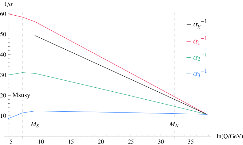
(a) $U(1)_{\chi}$

(b) $U(1)_{\psi}$

(c) $U(1)_{N}$

(d) $U(1)_{\eta}$

Figure 1: Gauge coupling unification in $E_{6}$ models. In all cases $M_{GUT}=2.4\times{10^{16}}$ GeV with $g_{U}\simeq{1.09}$. Here $M_{SUSY}=10^{3}$ GeV, $M_{S}=8\times{10^{3}}$ GeV and $M_{N}=10^{14}$ GeV.

Using the mass scales and parameters as described above, we obtain values of the three SM gauge couplings within the range constrained by the experimental results. In Figure 1 we present their evolution together with the abelian factor corresponding to the $U(1)_{\chi},U(1)_{\psi},U(1)_{N},$ and $U(1)_{\eta}$ models respectively. As shown in the figure, the decoupling of $U(1)$ is assumed at the mass scale $M_{S}=8$ TeV. The beta coefficient of the extra $U(1)$ gauge coupling depends on the corresponding charge as follows:

$$b_{\chi}=163/20,\quad b_{\psi}=25/3,\quad b_{N}=163/20,\quad b_{\eta}=227/30.$$ (13)

By assuming unification at $M_{GUT}=2.4\times{10^{16}}$ GeV we obtain the following values for the extra gauge coupling at the scale $M_{S}=8$ TeV :

$$g_{\chi}(M_{S})\simeq{0.508},\quad g_{\psi}(M_{S})\simeq{0.506},\quad g_{N}(M_{S})\simeq{0.508},\quad g_{\eta}(M_{S})\simeq{0.506}.$$ (14)

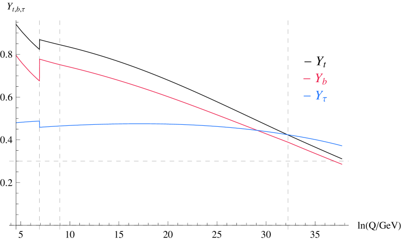
(a) $U(1)_{\chi}$

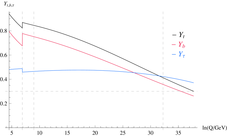
(b) $U(1)_{\psi}$

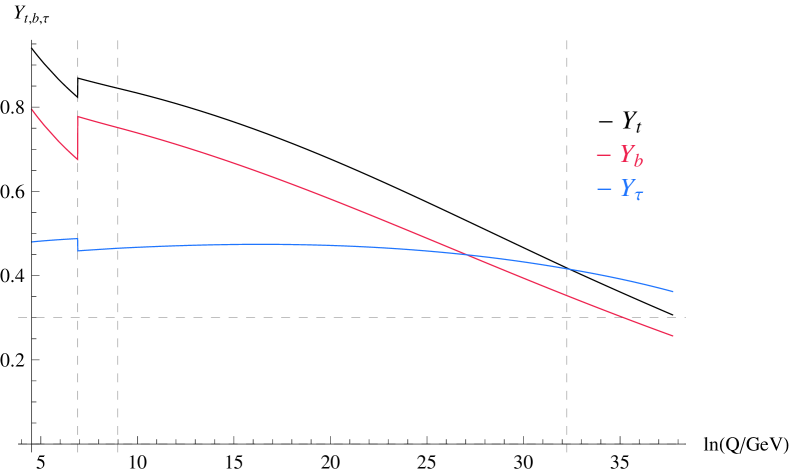
(c) $U(1)_{N}$

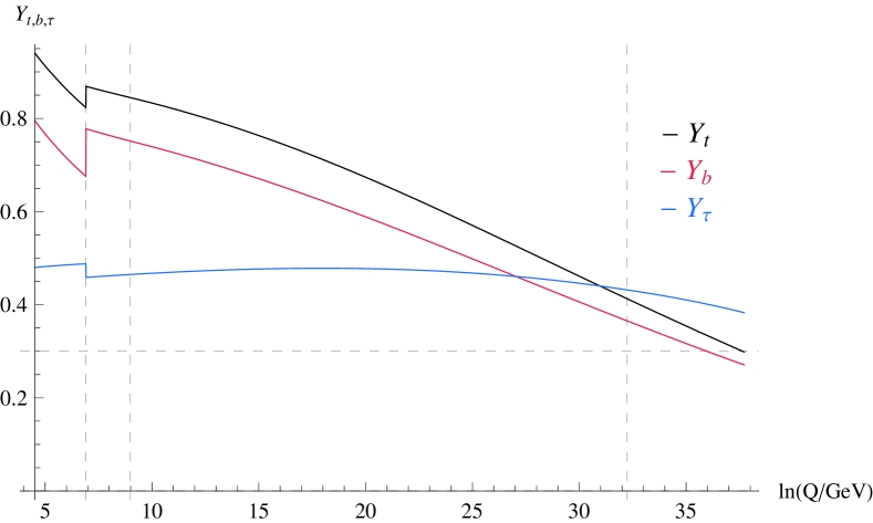
(d) $U(1)_{\eta}$

Figure 2: Running of t-b-$\tau$ Yukawa couplings. The horizontal dashed line corresponds to Y=0.3 and is used here for guidance. Here $tan\beta=50$, $|\mu|=0.5$ TeV and $A_{t}=2.2$ TeV.

Next we proceed with the Yukawa sector. In Figures 2 and 3 we present the evolution of the third generation Yukawa couplings for $\tan\beta=50$. Figure 2 corresponds to $|\mu|=0.5$ TeV and Figure  3 to $|\mu|=0.8$ TeV. In both cases, the masses of the sfermions were taken in the range of $2-3$ TeV and the trilinear parameter $A_{t}=2.2$ TeV. We observe that, in contrast to the minimal spectrum, in the presence of additional vectorlike matter, a moderate value of the top Yukawa coupling at the GUT-scale can reproduce the top mass at the electroweak scale. Furthermore, comparing Figures 2 and 3, we see that an increment of the SUSY threshold corrections and the value of $|\mu|$, implies larger GUT values of the Yukawa couplings. Some representative values for the same SUSY parameters but two different values of $\mu$ are presented in Tables 6 and 7. Our findings show that the results are the same for $\chi$ and $N$ models. For a discussion of sparticle spectroscopy with t-b-$\tau$ Yukawa unification see [30] and references therein.

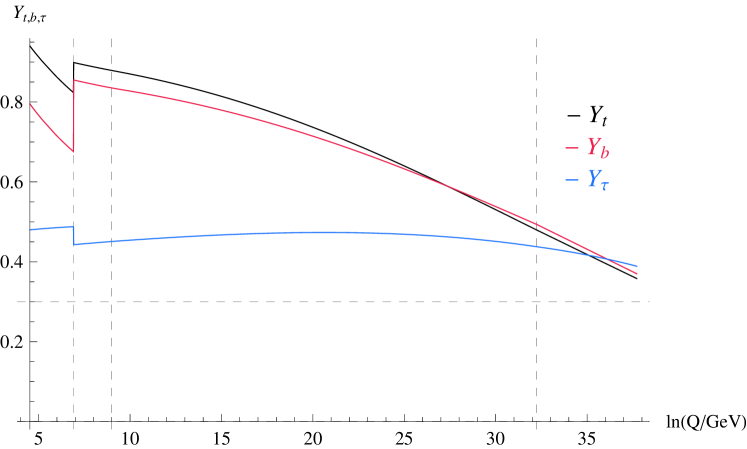
(a) $U(1)_{\chi}$

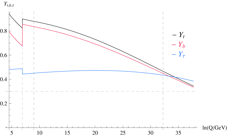
(b) $U(1)_{\psi}$

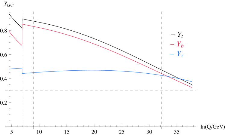
(c) $U(1)_{N}$

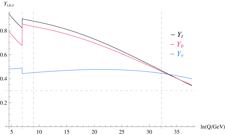
(d) $U(1)_{\eta}$

Figure 3: Running of t-b-$\tau$ Yukawa couplings. The horizontal dashed line corresponds to Y=0.3 and is used here for guidance. Here $tan\beta=50$, $|\mu|=0.8$ TeV and $A_{t}=2.2$ TeV.

We close this section with a few observations. First, we notice that raising the scale $M_{S}$ by a few TeV increases slightly the value of the Yukawa couplings. At the same time we get a lower value of the gauge coupling $g_{U}$ at $M_{GUT}$.

$E_{6}$ model	$Y_{t}$	$Y_{b}$	$Y_{\tau}$	$Y_{H}$	$Y_{D}$
$U(1)_{\chi}$	0.305	0.257	0.361	0.336	0.306
$U(1)_{\psi}$	0.300	0.262	0.370	0.330	0.300
$U(1)_{N}$	0.305	0.257	0.361	0.336	0.306
$U(1)_{\eta}$	0.297	0.270	0.380	0.345	0.324

Table 6: Numerical values of the Yukawa couplings at $M_{GUT}$ for $\tan\beta=50$ and $|\mu|=0.5$ TeV. The last two columns refer to the Yukawa couplings of the vectorlike pairs.

The $Z^{\prime}$ boson mass for the various models discussed above are as follows:

$$M_{Z_{\psi}}\approx 4.67\;{\rm TeV},\;\;M_{Z_{N}}\approx 4.54\;{\rm TeV},\;M_{Z_{\eta}}\approx 3.70\;{\rm TeV}.$$ (15)

In all cases, the predicted mass of $Z^{\prime}$ lies just above the current experimental bounds given by [4, 5, 6]

$$M^{exp}_{Z^{\prime}}\,>\,3.4-4.1\,{\rm TeV}~{}.$$

$E_{6}$ model	$Y_{t}$	$Y_{b}$	$Y_{\tau}$	$Y_{H}$	$Y_{D}$
$U(1)_{\chi}$	0.350	0.326	0.374	0.361	0.350
$U(1)_{\psi}$	0.342	0.333	0.383	0.372	0.358
$U(1)_{N}$	0.350	0.326	0.374	0.361	0.350
$U(1)_{\eta}$	0.340	0.345	0.396	0.372	0.371

Table 7: Numerical values of the Yukawa couplings at the GUT scale for $\tan\beta=50$ and $|\mu|=0.8$ TeV. The last two columns refer to the Yukawa couplings of the third family vectorlike pairs.

Next we discuss the extra doublet and vectorlike color triplet fields. As an example, following [25], we assume that the Yukawa couplings, $Y_{H}$ and $Y_{D}$, of one pair $H_{u}+H_{d}$ and one pair $D+\bar{D}$, unify asymptotically with the Yukawa couplings of the third generation at the GUT scale. The values of these couplings at the GUT scale are also presented in Tables 6 and 7. Using the RGE’s we predict the value at the scale $M_{S}$. We find that the masses of $D+\bar{D}$ and the extra $H_{u}+H_{d}$ doublets are:

$$m_{D} \geq{5.92}\quad\text{TeV},$$ (16)

$$m_{H} \geq{3.44}\quad\text{TeV}.$$ (17)

Finally, in our analysis we have found that in the presence of extra vectorlike pairs and singlet fields at a few TeV scale, the third generation fermion masses and in particular the top-mass can be correctly reproduced with moderate values of the Yukawa couplings at the GUT scale. As we will show, this is in agreement with the predictions from F-theory computations.

4.1 Yukawa Couplings in F-Theory

In F-theory, the Yukawa couplings are realised when three Riemann surfaces accommodating matter fields intersect at a single point on the GUT surface, $S$. Given the specific geometry of the compact space, we can solve the appropriate equations of motion and determine the profile of the wavefunctions of the states involved. The Yukawa couplings are then obtained by computing the integral of the overlapping wavefunctions at the triple intersections. The final result of the computation depends on local flux densities permeating the matter curves. In the present work, we consider an $E_{8}$ point of enhancement and follow the procedures described in a series of papers [31]-[36]. We should note that the flux units considered in Section 2 are integer valued as they arise from the Dirac quantisation

$$\frac{1}{2\pi}\int_{\Sigma\subset{S}}F=n_{f}\,,$$ (18)

where $n_{f}$ is an integer, $\Sigma$ denotes a matter curve (two-cycle in the divisor $S$), and $F$ is the gauge field strength tensor, i.e., the flux. In the same section we also described how the flux units piercing different matter curves $\Sigma$ determine the chiral states which are globally present in a given model. However, while the flux units in Section 2 define the full spectrum of the model, the study of the trilinear couplings involve the calculation of the wavefunctions and their overlaps on a local, approximately flat patch around a point of intersection. In this local approach it is the local values of flux -and not the global quantisation constraints- that matter. The local fluxes determine the chiral states at the local point. Besides those, there can be additional chiral fermions localised in other regions of the matter curve, with the total chirality determined by the integral of the magnetic flux along the matter curve. The relation between local and global fluxes is not a clear issue since it requires a complete knowledge of the geometry of the matter curve. A more sophisticated local vs. global analysis is given in [35]. In our present approach, we will consider ranges of flux densities corresponding to a wide range of integer values encompassing also those flux parameters used in section 2.

Following the formulation of [36] (see also [37]) we deal with two types of flux density parameters. The first type is parametrised by the flux density numbers $M_{i}$, $N_{i}$ where $i=1,2$, and descend from a worldvolume flux which is necessary to induce chirality on the matter curves accommodating the $10$-plets, $\bar{5}$-plets and $5$-plets of $SU(5)_{GUT}$. The second type parametrised by $N_{Y}$ and $\tilde{N}_{Y}$, is related to the hypercharge flux which breaks the $SU(5)$ symmetry to the Standard Model and in addition generates the observed chirality of the fermion families.

In Figure 4 we plot the bottom, tau and top Yukawa coupling at the local flux-density parameter space $M_{1}$ and $N_{Y}$. For the remaining flux density parameters involved in the computation we consider the values $N_{1}=0.187,M_{2}=1.23,N_{2}=0.701,\tilde{N}_{Y}=0.09$. For a reasonable range of the $M_{1}$ and $N_{Y}$ parameters, the values of $Y_{t,b,\tau}$ lie approximately between $0.3$ and $0.4$. There is a single $(M_{1},N_{Y})$ point (shown with green color bullet in Figure 4) where all Yukawa couplings of the third generation attain the same value $Y_{t,b,\tau}=0.35$.

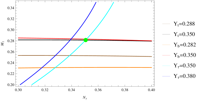
Figure 4: Values of the Yukawa couplings from the $E_{8}$ point in F-theory without imposing any constraint on the flux parameters. Green point corresponds to $Y_{t}\approx{Y_{b}}\approx{Y_{\tau}}=0.35$.

Before closing this section, we make a few comments regarding the issues emerging from supersymmetry breaking, such as soft masses and flavour changing neutral currents (FCNC). The structure of the SUSY breaking soft terms have been studied for a large class of string and flux compactifications with a MSSM-like spectrum [38]-[42]. In many cases the presence of non-diagonal flavor dependent SUSY-breaking soft terms are generically induced. The presence of such terms can lead to dangerous FCNC effects which can create tension with other phenomenological predictions of the low energy theory. In the case of F-theory generalisations, SUSY breaking soft terms and its phenomenological implications have been extensively discussed in the past [43]-[47], [34]. Especially in [46], [47], it is shown how SUSY breaking soft terms for fields on matter curves are generated from closed string fluxes, applying the results on F-theory local models and including contributions from magnetic fluxes. In the special case of non-constant fluxes flavor dependent soft terms arise which must lie in the multi-TeV range in order to avoid FCNC effects. However, the results strongly depend on the internal geometry, the background fluxes and there is considerable uncertainty from model dependent factors. On the other hand these flavor violating effects may be suppressed if the close string fluxes vary slowly over $S$.

Gravity mediated SUSY breaking is also a possible source of FCNC after integrating out heavy modes. In F-theory local models this scenario has been discussed in [34] where it is shown that off-diagonal terms are not induced due to the presence of geometric $U(1)$ symmetries, while a full study of FCNC requires the study of the difference $m^{2}_{22}-m_{11}^{2}$ of the soft scalar masses $m_{ij}$. We expect that this will be suppressed for a wide range of the parameter space while a detailed computation is beyond the scope of this letter.

5 Conclusions

In this work, we have presented effective field theory models embedded in $E_{6}$ with an extra neutral gauge boson ($Z^{\prime}$) and additional vectorlike fields in the low energy spectrum. The extra matter fields (beyond the MSSM spectrum), assumed to remain at the TeV region include triplets and doublets comprising three complete $5+\bar{5}$-plets of $SU(5)$, as well as neutral singlets. It is shown that this spectrum can be embedded naturally in an F-theory scenario where abelian fluxes are used to break the $E_{6}$ symmetry to $SU(5)$. Using renormalisation group analysis at two-loop level, we explore the implications of this spectrum on the running of the gauge and Yukawa couplings. We perform this analysis by assuming a $Z^{\prime}$ boson mass compatible with the LHC bounds and masses of the extra fields $\sim$ 10 TeV, and we take into account threshold corrections of SUSY particles and a right-handed neutrino scale $10^{14}$ GeV. We find that moderate values at the GUT scale of the third generation Yukawa coulings in the range $Y_{t,b,\tau}\sim 0.3-0.4$ and $\tan\beta\sim 50$ can successfully reproduce their low energy masses. Finally, based on previous detailed work on Yukawa couplings in F-theory [31]-[36], we compute the third generation Yukawa couplings generated by a configuration of intersecting seven-branes with the GUT divisor. We assume a configuration with a single $E_{8}$ point of enhancement and compute the relevant integral taking into account non-trivial fluxes associated with the symmetry breaking. We express the results in terms of the local flux densities and find that their values are in the same range with those found by the renormalisation group analysis using as inputs the known low energy masses of the charged fermions of the third family. We also find points in the parameter space of the flux densities where $t-b-\tau$ Yukawa couplings attain a common value.

Acknowledgements. G.K.L. would like to thank the Physics and Astronomy Department and Bartol Research Institute of the University of Delaware, and LPTHE of UPMC in Paris, for kind hospitality where part of this work has been done. Q.S. is supported in part by the DOE grant DE-SC0013880.

References

- [1] M. Cvetic, D. A. Demir, J. R. Espinosa, L. L. Everett and P. Langacker, Phys. Rev. D 56 (1997) 2861 Erratum: [Phys. Rev. D 58 (1998) 119905] doi:10.1103/PhysRevD.56.2861, 10.1103/PhysRevD.58.119905 [hep-ph/9703317].
- [2] P. Langacker, Rev. Mod. Phys. 81 (2009) 1199 doi:10.1103/RevModPhys.81.1199 [arXiv:0801.1345 [hep-ph]]; T. G. Rizzo, hep-ph/0610104; P. Athron, S. F. King, D. J. Miller, S. Moretti and R. Nevzorov, Phys. Lett. B 681 (2009) 448 doi:10.1016/j.physletb.2009.10.051 [arXiv:0901.1192 [hep-ph]].
- [3] M. Cvetic, J. Halverson and P. Langacker, JHEP 1111 (2011) 058 doi:10.1007/JHEP11(2011)058 [arXiv:1108.5187 [hep-ph]].
- [4] V. Khachatryan et al. [CMS Collaboration], Phys. Lett. B 773 (2017) 563 doi:10.1016/j.physletb.2017.08.069 [arXiv:1701.01345 [hep-ex]].
- [5] M. Aaboud et al. [ATLAS Collaboration], arXiv:1703.09127 [hep-ex].
- [6] The ATLAS collaboration [ATLAS Collaboration], ATLAS-CONF-2017-027.
- [7] F. Gursey, P. Ramond and P. Sikivie, Phys. Lett. 60B (1976) 177. doi:10.1016/0370-2693(76)90417-2
- [8] Y. Achiman and B. Stech, Phys. Lett. 77B (1978) 389. doi:10.1016/0370-2693(78)90584-1
- [9] Q. Shafi, Phys. Lett. 79B (1978) 301. doi:10.1016/0370-2693(78)90248-4
- [10] C. Beasley, J. J. Heckman and C. Vafa, JHEP 0901 (2009) 058 doi:10.1088/1126-6708/2009/01/058 [arXiv:0802.3391 [hep-th]]; C. Beasley, J. J. Heckman and C. Vafa, JHEP 0901 (2009) 059 doi:10.1088/1126-6708/2009/01/059 [arXiv:0806.0102 [hep-th]]; V. Bouchard, J. J. Heckman, J. Seo and C. Vafa, JHEP 1001 (2010) 061 doi:10.1007/JHEP01(2010)061 [arXiv:0904.1419 [hep-ph]].
- [11] J. C. Callaghan, S. F. King and G. K. Leontaris, JHEP 1312 (2013) 037 doi:10.1007/JHEP12(2013)037 [arXiv:1307.4593 [hep-ph]].
- [12] J. C. Callaghan, S. F. King, G. K. Leontaris and G. G. Ross, JHEP 1204 (2012) 094 doi:10.1007/JHEP04(2012)094 [arXiv:1109.1399 [hep-ph]].
- [13] C. M. Chen and Y. C. Chung, JHEP 1103, 129 (2011) doi:10.1007/JHEP03(2011)129 [arXiv:1010.5536 [hep-th]].
- [14] M. Cvetic, R. Donagi, J. Halverson and J. Marsano, JHEP 1211 (2012) 004 doi:10.1007/JHEP11(2012)004 [arXiv:1209.4906 [hep-th]].
- [15] G. K. Leontaris and Q. Shafi, Eur. Phys. J. C 76 (2016) no.10, 574 doi:10.1140/epjc/s10052-016-4432-y [arXiv:1603.06962 [hep-ph]].
- [16] P. Langacker and J. Wang, Phys. Rev. D 58 (1998) 115010 doi:10.1103/PhysRevD.58.115010 [hep-ph/9804428].
-
[17]
F. Staub,
Comput. Phys. Commun. 185 (2014) 1773
doi:10.1016/j.cpc.2014.02.018
[arXiv:1309.7223 [hep-ph]].
F. Staub, Adv. High Energy Phys. 2015 (2015) 840780 doi:10.1155/2015/840780 [arXiv:1503.04200 [hep-ph]]. - [18] L. E. Ibanez and J. Mas, Nucl. Phys. B 286 (1987) 107. doi:10.1016/0550-3213(87)90434-2
- [19] E. Ma, Phys. Lett. B 380 (1996) 286 doi:10.1016/0370-2693(96)00524-2 [hep-ph/9507348].
- [20] S. F. King, S. Moretti and R. Nevzorov, Phys. Rev. D 73 (2006) 035009 doi:10.1103/PhysRevD.73.035009 [hep-ph/0510419].
- [21] E. Witten, Nucl. Phys. B 258 (1985) 75. doi:10.1016/0550-3213(85)90603-0
- [22] P. Athron, D. Harries, R. Nevzorov and A. G. Williams, Phys. Lett. B 760 (2016) 19 doi:10.1016/j.physletb.2016.06.040 [arXiv:1512.07040 [hep-ph]].
- [23] P. Athron, A. W. Thomas, S. J. Underwood and M. J. White, Phys. Rev. D 95 (2017) no.3, 035023 doi:10.1103/PhysRevD.95.035023 [arXiv:1611.05966 [hep-ph]].
- [24] Y. Hicyilmaz, M. Ceylan, A. Altas, L. Solmaz and C. S. Un, Phys. Rev. D 94 (2016) no.9, 095001 doi:10.1103/PhysRevD.94.095001 [arXiv:1604.06430 [hep-ph]].
- [25] A. Hebbar, G. K. Leontaris and Q. Shafi, Phys. Rev. D 93 (2016) no.11, 111701 doi:10.1103/PhysRevD.93.111701 [arXiv:1604.08328 [hep-ph]].
- [26] Belangér, Geneviève, J. Da Silva and H. M. Tran, Phys. Rev. D 95 (2017) no.11, 115017 doi:10.1103/PhysRevD.95.115017 [arXiv:1703.03275 [hep-ph]].
- [27] J. Y. Araz, M. Frank and B. Fuks, Phys. Rev. D 96 (2017) no.1, 015017 doi:10.1103/PhysRevD.96.015017 [arXiv:1705.01063 [hep-ph]].
- [28] Y. Hicyilmaz, L. Solmaz, S. H. Tanyildizi and C. S. Un, arXiv:1706.04561 [hep-ph].
- [29] G. C. Cho, N. Maru and K. Yotsutani, Mod. Phys. Lett. A 31 (2016) no.22, 1650130 doi:10.1142/S0217732316501303 [arXiv:1602.04271 [hep-ph]].
- [30] M. A. Ajaib, I. Gogoladze, Q. Shafi and C. S. Ün JHEP 1405 (2014) 079 doi:10.1007/JHEP05(2014)079 [arXiv:1402.4918 [hep-ph]].
- [31] S. Cecotti, C. Cordova, J. J. Heckman and C. Vafa, JHEP 1107 (2011) 030 doi:10.1007/JHEP07(2011)030 [arXiv:1010.5780 [hep-th]].
- [32] G. K. Leontaris and G. G. Ross, JHEP 1102 (2011) 108 doi:10.1007/JHEP02(2011)108 [arXiv:1009.6000 [hep-th]].
- [33] L. Aparicio, A. Font, L. E. Ibanez and F. Marchesano, JHEP 1108 (2011) 152 doi:10.1007/JHEP08(2011)152 [arXiv:1104.2609 [hep-th]].
- [34] P. G. Camara, E. Dudas and E. Palti, JHEP 1112 (2011) 112 doi:10.1007/JHEP12(2011)112 [arXiv:1110.2206 [hep-th]].
- [35] E. Palti, JHEP 1207 (2012) 065 doi:10.1007/JHEP07(2012)065 [arXiv:1203.4490 [hep-th]].
- [36] F. Marchesano, D. Regalado and G. Zoccarato, JHEP 1504 (2015) 179 doi:10.1007/JHEP04(2015)179 [arXiv:1503.02683 [hep-th]].
- [37] M. Crispim Romão, A. Karozas, S. F. King, G. K. Leontaris and A. K. Meadowcroft, JHEP 1611 (2016) 081 doi:10.1007/JHEP11(2016)081 [arXiv:1608.04746 [hep-ph]].
- [38] A. Brignole, L. E. Ibanez and C. Munoz, Nucl. Phys. B 422 (1994) 125 Erratum: [Nucl. Phys. B 436 (1995) 747] doi:10.1016/0550-3213(94)00600-J, 10.1016/0550-3213(94)00068-9 [hep-ph/9308271].
- [39] M. Grana, T. W. Grimm, H. Jockers and J. Louis, Nucl. Phys. B 690 (2004) 21 doi:10.1016/j.nuclphysb.2004.04.021 [hep-th/0312232].
- [40] P. G. Camara, L. E. Ibanez and A. M. Uranga, Nucl. Phys. B 689 (2004) 195 doi:10.1016/j.nuclphysb.2004.04.013 [hep-th/0311241].; P. G. Camara, L. E. Ibanez and A. M. Uranga, Nucl. Phys. B 708 (2005) 268 doi:10.1016/j.nuclphysb.2004.11.035 [hep-th/0408036].
- [41] D. Lust, S. Reffert and S. Stieberger, Nucl. Phys. B 706 (2005) 3 doi:10.1016/j.nuclphysb.2004.11.030 [hep-th/0406092].
- [42] K. Choi, K. S. Jeong and K. I. Okumura, JHEP 0807 (2008) 047 doi:10.1088/1126-6708/2008/07/047 [arXiv:0804.4283 [hep-ph]].
- [43] L. Aparicio, D. G. Cerdeno and L. E. Ibanez, JHEP 0807 (2008) 099 doi:10.1088/1126-6708/2008/07/099 [arXiv:0805.2943 [hep-ph]].
- [44] J. J. Heckman and C. Vafa, JHEP 0909 (2009) 079 doi:10.1088/1126-6708/2009/09/079 [arXiv:0809.1098 [hep-th]].
- [45] R. Blumenhagen, J. P. Conlon, S. Krippendorf, S. Moster and F. Quevedo, JHEP 0909 (2009) 007 doi:10.1088/1126-6708/2009/09/007 [arXiv:0906.3297 [hep-th]]. [46]
- [46] P. G. Camara, L. E. Ibanez and I. Valenzuela, JHEP 1310 (2013) 092 doi:10.1007/JHEP10(2013)092 [arXiv:1307.3104 [hep-th]].
- [47] P. G. Camara, L. E. Ibanez and I. Valenzuela, JHEP 1406 (2014) 119 doi:10.1007/JHEP06(2014)119 [arXiv:1404.0817 [hep-th]].