OGLE-2016-BLG-0613LABb: A Microlensing Planet in a Binary System

Abstract

We present the analysis of OGLE-2016-BLG-0613, for which the lensing light curve appears to be that of a typical binary-lens event with two caustic spikes but with a discontinuous feature on the trough between the spikes. We find that the discontinuous feature was produced by a planetary companion to the binary lens. We find 4 degenerate triple-lens solution classes, each composed of a pair of solutions according to the well-known wide/close planetary degeneracy. One of these solution classes is excluded due to its relatively poor fit. For the remaining three pairs of solutions, the most-likely primary mass is about $M_{1}\sim 0.7\,M_{\odot}$ while the planet is a super-Jupiter. In all cases the system lies in the Galactic disk, about half-way toward the Galactic bulge. However, in one of these three solution classes, the secondary of the binary system is a low-mass brown dwarf, with relative mass ratios (1 : 0.03 : 0.003), while in the two others the masses of the binary components are comparable. These two possibilities can be distinguished in about 2024 when the measured lens-source relative proper motion will permit separate resolution of the lens and source.

1 Introduction

More than half of stars belong to binary or multiple systems (Abt, 1983). From high-resolution imaging observations of host stars of Kepler extrasolar planets, Horch et al. (2014) concluded that the overall binary fraction of the planet-host stars is similar to the rate for field stars, suggesting that planets in binary systems are likely to be as common as those around single stars. The environment of the protoplanetary disk around a star in a binary system would have been affected by the gravitational influence of the companion and thus planets in binary systems are expected to be formed through a different mechanism from that of single stars (Thebault & Haghighipour, 2015). However, the current leading theories about the planet formation such as the core-accretion theory (Ida & Lin, 2004) and the disk instability theory (Boss, 2006) have been mostly focused on single stars, and thus many aspects about the formation mechanism of planets in binary systems remain uncertain. In order to derive a clear understanding of the formation mechanism, a sample comprising a large number of planetary systems in various types of binary systems will be important.

Microlensing can provide a tool to detect planets in binaries. The method is important because it can detect planets that present significant difficulties for other major planet detection methods. Since the microlensing phenomenon occurs regardless of the light from lensing objects, it enables one to detect planets around faints stars or even dark objects (Mao & Paczyński, 1991; Gould & Loeb, 1992). While the transit method is sensitive to circumbinary planets, wherein the planet orbits both stars in a close binary, and the high-resolution imaging method is sensitive to circumstellar planets, wherein the planet orbits one star of a very wide binary system, the microlensing method can detect both populations of circumbinary (Han, 2008) and circumstellar planets (Lee et al., 2008; Han et al., 2016).

However, identifying microlensing planets in binary systems is a difficult task due to the complexity of triple-lensing light curves and the resulting complication in the analysis. When a lensing event is produced by a single mass, the resulting light curve has a simple smooth and symmetric shape which is described by 3 lensing parameters of the time of the closest approach of the source to the lens, $t_{0}$, which defines the time of the peak magnification, the lens-source separation at that time, $u_{0}$ (impact parameter), which determines the peak magnification of the event, and the Einstein time scale $t_{\rm E}$, which characterizes the duration of the event. When a lens is composed of multiple components, on the other hand, the lensing light curve becomes greatly complex.

The first cause of the light curve complexity is the increase of the parameters needed to describe the light curve. In order to describe the light curves produced by a binary lens, one needs 3 more parameters in addition to the single-lens parameters. These include the separation $s_{2}$ and mass ratio $q_{2}=M_{2}/M_{1}$ between the binary lens components and the source trajectory angle $\alpha$ with respect to the binary axis. Here $M_{1}$ and $M_{2}$ denote the masses of the primary and companion of the binary, respectively. For a triple-lens system, such as the case of a planet in a binary system, one needs to add 3 more parameters including the orientation angle $\psi$ of the third body $M_{3}$ and the separation $s_{3}$ and mass ratio $q_{3}$ between $M_{1}$ and $M_{3}$. In Figure 1, we provide the graphical presentation of the triple-lensing parameters used in our analysis. With the increased number of parameters, the parameter space to be explored in the analysis greatly increases, making the analysis of triple-lens system difficult.

The second major cause of the light curve complexity is the formation of caustics. Caustics refer to curves on the source plane at which lensing magnifications of a point source become infinite, and thus the lensing light curves produced by source star’s crossing over the caustic are characterized by sharp spikes. Caustics of a binary-lens systems form closed curves, in which the topology of caustic curves depends on the binary separation and mass ratio (Schneider & Weiss, 1986; Bozza, 1999; Dominik, 1999a). The addition of a third component to the lens system greatly increases the complexity of the caustic topology, and the loops of caustics may overlap and intersect, resulting in nested curves (Gaudi et al., 1998). As a result, the topology of the triple lens system has not yet been fully understood although there have been some studies on the caustics of a subset of triple lens systems, e.g., Danék & Heyrovský (2015) and Luhn et al. (2016).

Figure 1: Graphical presentation of the triple-lensing parameters.

Although very complex, microlensing light curves of some triple-lens systems can be readily analyzed. One such case is a planet in a binary system for which the masses of the stellar lens components overwhelm that of the planet, i.e. $M_{1}\sim M_{2}\gg M_{3}$. In this case, the overall shape of the lensing light curve is approximated by the binary-lens light curve of the $M_{1}$–$M_{2}$ pair, and the signal of the third body can be treated as a perturbation to the binary-lens curve.

There have been 5 triple lensing events published to date. These include OGLE-2006-BLG-109 (two planet system, Gaudi et al., 2008; Bennett et al., 2010), OGLE-2012-BLG-0026 (two planet system, Han et al., 2013; Beaulieu et al., 2016), OGLE-2013-BLG-0341 (circumstellar planetary system, Gould et al., 2014), OGLE-2008-BLG-092 (circumstellar planetary system, Poleski et al., 2014), and OGLE-2007-BLG-349 (circumbinary planetary system, Bennett et al., 2016). For OGLE-2006-BLG-109, the caustics induced by the two planets interfere each other and the resulting caustic pattern is complex, making the analysis difficult. For the other 4 cases, however, the interference is minimal and thus the resulting caustic can be approximated by the superposition of the caustics induced by the individual companions (Han, 2005). This enables to treat $M_{1}$–$M_{2}$ and $M_{1}$–$M_{3}$ pairs as independent binary systems, making the analysis simplified.

In addition, there are two cases in the literature of lens systems that were originally identified as triples and then were later recognized to be binary lenses: MACHO-97-BLG-41 (Bennett et al., 1999; Albrow et al., 2000; Jung et al., 2013; Ryu et al., 2017) and OGLE-2013-BLG-0723 (Udalski et al., 2015; Han et al., 2016). In both cases, the “additional” caustic that had been thought to be caused by an additional body (whose properties were then evaluated based on the above-mentioned principle of superposition) was actually a minor-image caustic that had moved during the event due to the orbital motion of the binary. The first case is particularly instructive. Soon after the triple model was introduced, Albrow et al. (2000) had developed an alternative (binary) model from the analysis based on a completely different data set which had additional data points and thus provided stronger constraints on the first caustic compared to the Bennett et al. (1999) study. Later, Jung et al. (2013) combined these data sets and showed that the binary model was strongly favored. Subsequently, Ryu et al. (2017) showed that the fundamental reason for the superiority of the binary model is that the orbtial-motion of the binary was already strongly present in the brief encounter of the source with the central caustic. In brief, triple lenses inhabit a wide range of parameter space, leading to considerably different levels of difficulty in analyzing them and disentangling them from binary lenses. While considerable progress has been made, much is still being learned.

In this work, we report a planet in a binary system that was detected from the analysis of the microlensing event OGLE-2016-BLG-0613. The overall light curve of the event appears to be consistent with that of a typical caustic-crossing binary-lens event with two strong spikes, but it exhibits a short-term discontinuous feature on the smooth ”U”-shape trough region between the caustic spikes. We find that the short-term feature is produced by a planet-mass companion to the binary lens.

The paper is organized as follows. In Section 2, we discuss the observation of the lensing event and the data acquired from it. In Section 3, we describe the procedures of modeling the observed lensing light curve and estimate the physical parameters of the lens system. In Section4, we discuss the scientific importance of the lensing event. We summarize the results and conclude in Section 5.

2 Data

The microlensing event OGLE-2016-BLG-0613 occurred on a star located toward the Galactic bulge field. The equatorial coordinates of the source star are $(\alpha,\delta)_{\rm J2000}=(17^{\rm h}57^{\rm m}02^{\rm s}\hskip-2.0pt.50,-28^{\circ}06^{\prime}58^{\prime\prime}\hskip-2.0pt.2)$. The corresponding Galactic coordinates are $(l,b)=(1^{\circ}\hskip-2.0pt.99,-1^{\circ}\hskip-2.0pt.74)$, which is very close to the Galactic center. The event was discovered by the Early Warning System (Udalski, 2003) of the Optical Gravitational Lensing Experiment (OGLE: Udalski et al., 2015) survey, which monitors the Galactic bulge field using the 1.3m Warsaw telescope at the Las Campanas Observatory in Chile. The discovery of the event was announced on 2016 April 11. Most of the OGLE data were taken in the standard Cousins $I$ band and some $V$-band images were taken for color measurement.

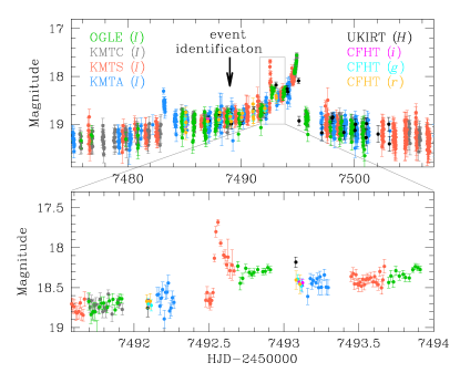
Figure 2: Light curve of OGLE-2016-BLG-0613. The lower panel shows the enlarged view of the short-term discontinuous anomaly that occurred at ${\rm HJD}\sim 2457493$. The arrow in the upper panel denotes the time when the event was identified.

The event was also in the field of the Korea Microlensing Telescope Network (KMTNet: Kim et al., 2016) survey, which monitors the bulge field using 3 globally distributed telescopes located at the Cerro Tololo Interamerican Observatory in Chile (KMTC), the South African Astronomical Observatory in South Africa (KMTS), and the Siding Spring Observatory in Australia (KMTA). The aperture of each telescope is 1.6m. The camera, which is composed of 4 chips, provides a 4-deg² field of view. The event OGLE-2016-BLG-0613 was in one of the three major fields toward which observations were conducted with 15-minute cadence. For these major fields, the KMTNet survey conducts alternating observations with 6-arcminute offset in order to cover the gaps between chips of the camera. As a result, the KMTNet data are composed of two sets (denoted by “BLG02” and “BLG42”). KMTNet observations were also conducted in the standard Cousins $I$ band with occasional observations in $V$ band.

The event was also observed by the surveys conducted using the 3.8m United Kingdom Infrared Telescope (UKIRT Microlensing survey: Shvartzvald et al., 2017) and the 3.6m Canada France Hawaii Telescope (CFHT). Both telescopes are located at the Mauna Kea Observatory in Hawaii. UKIRT observations were conducted in $H$ band and the images from CFHT observations were taken in $i$, $r$, and $g$ bands.

In Figure 2, we present the light curve of OGLE-2016-BLG-0613. At the time of being identified (${\rm HJD}^{\prime}={\rm HJD}-2450000\sim 7489$), the light curve of the event already showed deviations from the smooth and symmetric form of a point-mass event. With the progress of the event, the light curve exhibited a “U”-shape trough, which is a characteristic feature that appears when a source star passes through the inner region of the caustic formed by a binary lens. Caustics of a binary lens form closed curves, and thus caustic crossings occur in pairs. The first caustic spike, which occurred at ${\rm HJD}^{\prime}\sim 7483$, was inferred from the trough feature of the OGLE data and identified later by the KMTA data. The second caustic spike occurred at ${\rm HJD}^{\prime}\sim 7495$. The “baseline object” of the event was very faint with a baseline magnitude $I_{\rm OGLE}\sim 19.4$. Furthermore, the baseline of the light curve showed a systematic trend of declination. As a result, the event drew little attention and thus it was not covered by follow-up observations.

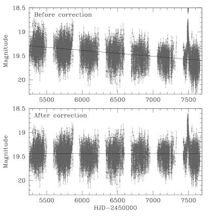
Figure 3: Systematic trend in the OGLE baseline data. The upper and lower panels show the data before and after the correction, respectively.

Preliminary analysis of the event was done as a part of real-time modeling efforts that were conducted to check the scientific importance of anomalous events. From this, it was noticed that there exists a short-term discontinuous feature at ${\rm HJD}^{\prime}\sim 7493$ in a U-shape trough region between the caustic spikes. We present the enlarged view of the anomaly in the lower panels of Figure 2. Successive modeling of the light curve conducted with the progress of the event yielded solutions that can describe the overall light curve. However, the short-term anomaly could not be explained by models based on the binary-lens interpretation. See more discussion in Section 3.

Photometry of the images taken from observations were conducted by using various versions of codes developed based on the the difference imaging analysis method (DIA: Alard & Lupton, 1998). The OGLE data were processed with the customized pipeline (Udalski, 2003). The UKIRT data, which were taken in $H$ band, were also reduced with the DIA technique. The data taken by the KMTNet and CFHT surveys were reduced with customized versions of PySIS (Albrow et al., 2009) and ISIS, respectively.

Table 1: Error bar correction factors

Data set		$N$	$k$	$\sigma_{\rm min}$
OGLE		1924	1.68	0.001
KMTC	(BLG02 Field)	292	1.45	0.001
–	(BLG42 Field)	363	1.46	0.001
KMTS	(BLG02 Field)	675	1.51	0.001
–	(BLG42 Field)	630	1.93	0.001
KMTA	(BLG02 Field)	397	1.40	0.001
–	(BLG42 Field)	383	1.34	0.001
UKIRT		71	1.41	0.020
CFHT	(i band)	44	1.43	0.020
–	(r band)	47	1.78	0.020
–	(g band)	45	1.25	0.020

As mentioned, the baseline of the event exhibits a systematic trend by which the baseline magnitude gradually increases. See the upper panel of Figure 3, which shows the 7 year baseline since 2010. Such a trend is often produced by a blended star that is moving away from the source star, e.g. OGLE-2013-BLG-0723 (Han et al., 2016). As the blend moves away, less flux is included within the tapered aperture of photometry for the source flux measurement, causing declining baseline. We remove the trend by conducting a linear fit to the baseline. See the light curve after the baseline correction presented in the lower panel of Figure 3.

For the analysis of the data taken from different telescopes and processed using different photometry codes, we readjust error bars of each data set following the usual procedure described in Yee et al. (2012), i.e.

$$\sigma=k(\sigma_{0}^{2}+\sigma_{\rm min}^{2})^{1/2}.$$ (1)

Here $\sigma_{0}$ denotes the error bar estimated from the photometry pipeline, $\sigma_{\rm min}$ is a factor used to make the error bars be consistent with the scatter of data, and $k$ is the scaling factor used to make $\chi^{2}/{\rm dof}=1$. The adopted values of the error-bar correction factors $k$ and $\sigma_{\rm min}$ are listed in Table 1. Also presented is the number of data points, $N$, for the individual data sets.

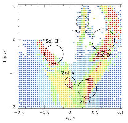
Figure 4: $\Delta\chi^{2}$ map in the $\log s$–$\log q$ parameter space. The encircled regions represent the locations of the 5 local binary-lens solutions. The color coding represent points in the MCMC chain within $1n\sigma$ (red), $2n\sigma$ (yellow), $3n\sigma$ (green), $4n\sigma$ (cyan), and $5n\sigma$ (blue), where $n=8$.

3 Analysis

3.1 Binary-Lens Modeling

Since the sharp spikes in the lensing light curve are characteristic features of caustic-crossing binary-lens events, we start modeling of the light curve based on the assumption that the lens is composed of two masses, $M_{1}$ and $M_{2}$. For the simple case in which the relative lens-source motion is rectilinear, the light curve of a binary-lens event is described by 7 geometric parameters plus 2 parameters representing the fluxes from the source, $F_{s}$, and blend, $F_{b}$, for each data set. The geometric lensing parameters include 3 of a single-lens event ($t_{0}$, $u_{0}$ and $t_{\rm E}$), another 3 parameters describing the binary lens ($s$, $q$, and $\alpha$), and the ratio of the angular source radius $\theta_{*}$ to the angular Einstein radius $\theta_{\rm E}$, i.e. $\rho=\theta_{*}/\theta_{\rm E}$ (normalized source radius). The lengths of $u_{0}$ and $s$ are normalized to $\theta_{\rm E}$.

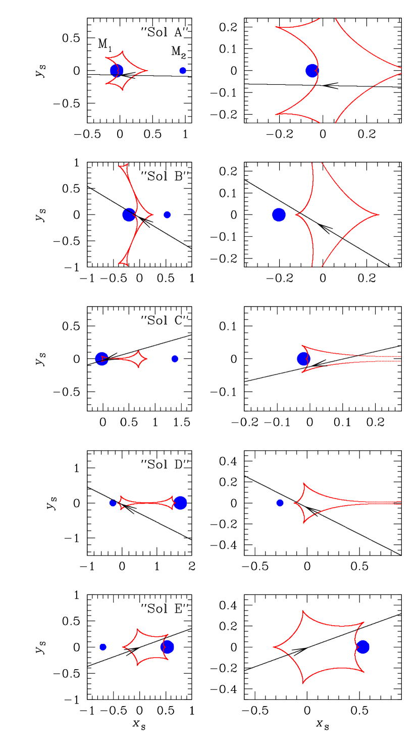
Figure 5: Caustic geometry of the 5 local binary-lens solutions. For each local, the left panel shows the whole view and the right panel shows the zoom of the caustic-crossing region. In each panel, the cuspy closed curve represents the caustic and the line with an arrow is the source trajectory. The blue dots represent the lens components where the bigger and smaller dots denote the primary ($M_{1}$) and companion ($M_{2}$), respectively.

In the preliminary binary-lens modeling, we first conduct a grid search over the parameter space of $s$, $q$, and $\alpha$, while the remaining parameters ($t_{0}$, $u_{0}$, $t_{\rm E}$, and $\rho$) are searched for using a downhill approach. We choose $s$, $q$, and $\alpha$ as the grid parameters because lensing magnifications vary sensitively to the small changes of these parameters. For the downhill approach, we use the Markov Chain Monte Carlo (MCMC) method. The initial values of the MCMC parameters are roughly guessed considering the characteristics of the light curve such as the duration, caustic crossing times, etc. From the preliminary search, we find that (1) there exist multiple local minima that can describe the overall feature of the light curve but (2) none of these solutions can explain the short-term anomaly at ${\rm HJD}^{\prime}\sim 7493$.

Table 2: Local binary-lens solutions

Parameters	‘Sol A’	‘Sol B’	‘Sol C’	‘Sol D’	‘Sol E’
$\chi^{2}$	9212.4	9185.7	9179.2	9183.6	9195.1
$t_{0}$ (HJD’)	7493.443 $\pm$ 0.055	7490.032 $\pm$ 0.053	7493.872 $\pm$ 0.054	7490.004 $\pm$ 0.081	7486.311 $\pm$ 0.109
$u_{0}$	0.069 $\pm$ 0.001	0.046 $\pm$ 0.001	0.023 $\pm$ 0.001	0.039 $\pm$ 0.001	-0.006 $\pm$ 0.007
$t_{\rm E}$ (days)	44.63r $\pm$ 0.39	52.87 $\pm$ 0.66	74.09 $\pm$ 0.20	53.39 $\pm$ 0.40	17.15 $\pm$ 0.20
$s$	1.011 $\pm$ 0.006	0.730 $\pm$ 0.006	1.393 $\pm$ 0.003	1.926 $\pm$ 0.008	1.228 $\pm$ 0.006
$q$	0.050 $\pm$ 0.002	0.382 $\pm$ 0.005	0.026 $\pm$ 0.001	1.002 $\pm$ 0.081	6.032 $\pm$ 0.002
$\alpha$ (rad)	3.157 $\pm$ 0.010	3.681 $\pm$ 0.009	2.915 $\pm$ 0.008	3.611 $\pm$ 0.012	-0.348 $\pm$ 0.016
$\rho$ ($10^{-3}$)	0.21 $\pm$ 0.07	0.21 $\pm$ 0.04	0.31 $\pm$ 0.04	0.31 $\pm$ 0.05	0.31 $\pm$ 0.02

Note. — ${\rm HJD}^{\prime}={\rm HJD}-2450000$.

It is a well known fact that there can exist multiple degenerate solutions in binary lensing modeling due to deep symmetries in the lens equation (Griest & Safizadeh, 1998; Dominik, 1999b; An, 2005). There is also at least one well-studied “accidental” degeneracy between binary light curves due to planetary-mass and roughly equal-mass binaries, which does not occur for any deep reason (Choi et al., 2012; Bozza et al., 2016). However, the general problem of “accidental” degeneracies is poorly studied. One general principle, however, is that the lower the quality and quantity of data, the wider is the range of possible binary geometries that may fit the data reasonably well. As seen from Figure 2, OGLE-2016-BLG-0613 was exceptionally faint for a planet-bearing microlensing event, never getting brighter than $I\sim 17.5$. Moreover, although it was overall densely covered, by chance both the binary caustic entrance (${\rm HJD}^{\prime}\sim 7483$) and exit (${\rm HJD}^{\prime}\sim 7495$) fell in the gap between KMTC and KMTA coverage. Hence, there is a total of only one data point (from UKIRT) on these features. Binary events whose caustics lack such coverage are rarely, if ever, intensively studied, so that little is known about how they are impacted by “accidental” degeneracies. Therefore, one must pay particular attention to identifying all degenerate topologies.

Although several local solutions are found from the preliminary grid search, some local solutions might be still missed possibly due to a poor guess of the initial values of the MCMC parameters or some other reasons. We, therefore, check the existence of additional local solutions using two systematic approaches.

In the first approach, we conduct a series of additional grid searches in which we provide various combination of MCMC parameters as initial values. For a single lensing event, the values of the MCMC parameters are well characterized by the peak time (for $t_{0}$), peak magnification (for $u_{0}$), and the duration of the event (for $t_{\rm E}$). For OGLE-2016-BLG-0613, however, it is difficult to estimate these values from the light curve and thus it might be that some local solutions have been missed if the given initial parameters were too far away from the correct ones. From these searches, we identify 5 local solutions. Among them, 2 local solutions were missed in the initial search mainly due to the large difference between the Einstein time scales given as an initial value and the recovered value from modeling.

In the second approach, we directly consider each of 21 different caustic topologies that are consistent with the overall morphology of the light curve. As seen in Figure 2, the caustic structures appear near the peak of the pre-caustic plus post-caustic light curve. The caustic structure must therefore be either a four-sided (“central”) caustic or a six-sided (“resonant”) caustic. Allowing for the symmetry of these caustic structures around the binary axis, there are $(4/2)\times(4-1)=6$ topologically distinct source paths for the central caustic and $(6/2)\times(6-1)=15$ for the resonant caustic. We seed each of these topologies with an arbitrary $(s,q)$ geometry (that permits such a path) and set initial values of $(t_{0},u_{0},t_{\rm E},\alpha)$ such that the caustic entrance and exit occur at approximately the correct times. We then allow all parameters to vary using $\chi^{2}$ minimization. Although the initial seed solutions generally provide extremely poor matches to the data, the derived local minima are always in rough accord with the data, showing that the approach is working. Nevertheless, only four of these solutions have $\chi^{2}$ within a few hundred of the global minimum. These yield the same five solutions found by the grid searches above, with one of the four topology solutions corresponding to a close-wide pair of grid-search solutions. See below.

In Figure 4, we present the locations of the local solutions in the $\Delta\chi^{2}$ map of the $\log s$ – $\log q$ parameter space. The individual local solutions are marked by circles and labeled as ‘Sol A’, ‘Sol B’, ‘Sol C’, ‘Sol D’, and ‘Sol E’, respectively. In Table 2, we present the lesing parameters of the individual local binary-lensing solutions. In Figure 5, we also present the geometry of the lens systems, which show the source trajectory with respect to the positions of the lens components and caustics. One finds that the lensing parameters of the local solutions span over wide ranges. For example, the range of the binary mass ratio is $0.03\lesssim q\lesssim 6.0$. This implies that the observed light curve is serendipitously described by multiple local solutions with widely different lensing parameters.

Although the overall shape of the observed light curve is described by multiple solutions, none of the solutions can explain the short-term anomaly at ${\rm HJD}^{\prime}\sim 7493$. The anomaly is unlikely to be caused by systematics in the data because the feature was covered commonly by the OGLE, KMTS, KMTA, and UKIRT data. The region between caustic spikes can deviate from a smooth U shape if the source within the caustic asymptotically approaches the caustic curve. In such a case, however, the deviation occurring during the caustic approach is smooth, while the observed short-term anomaly appears to be a small-scale caustic-crossing feature composed of both caustic entrance (at ${\rm HJD}^{\prime}\sim 7292.5$) and exit (${\rm HJD}^{\prime}\sim 7293.1$) and the U-shape trough between them.

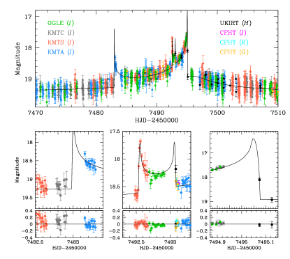
Figure 6: Model light curve of a triple-lens solution. The upper panel shows the model fit for the overall light curve, while the lower 3 panels show the fits for the caustic-crossing regions. We note that the presented model light curve is that of ‘Sol B’ and that ‘Sol C (wide)’ and ‘Sol D’ provide models with similar fits.

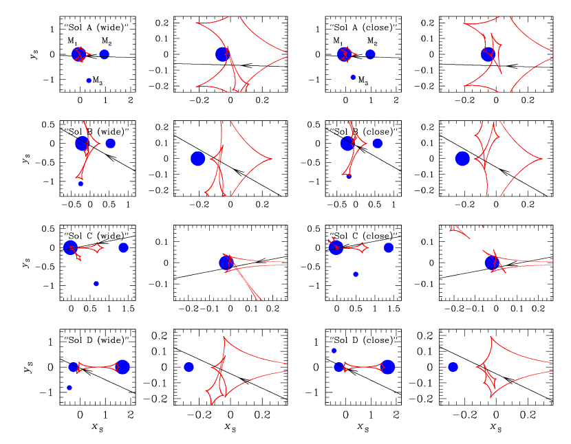
Figure 7: Caustic geometry of the 4 local triple-lens solutions. For each of the solutions, marked by ‘Sol A’, ‘Sol B’, ‘Sol C’, and ‘Sol D’, a pair of solutions, which are marked by ‘close’ and ‘wide’, resulting from the close/wide degeneracy of the third body are presented. Notations are same as those in Fig. 5.

3.2 Triple-Lens Modeling

Binary lenses form closed curves, it is mathematically impossible for a binary lens to generate two successive caustic entrances without an intervening caustic exit, nor similarly two successive caustic exits without an intervening caustic entrance. In the present case, we have both two such successive entrances followed by two such successive exits. This suggests that one should consider a new interpretation of the event other than the binary-lens interpretation.

It is known that a third body of a lens can cause caustic curves to be self-intersected (Schneider et al., 1992; Petters et al., 2001; Danék & Heyrovský, 2015; Luhn et al., 2016), and the light curve resulting from the source trajectory passing over the intersected part of the caustic can result in an additional caustic-crossing feature within the major caustic feature. We therefore conduct a triple-lens modeling of the observed light curve in order to check whether the short-term anomaly can be explained by a third body.

The 3-body lens modeling is conducted in two steps. In the first step, we conduct a grid search for the parameters related to the third body ($s_{3}$, $q_{3}$, and $\psi$) by fixing the binary-lens parameters at the values obtained from the binary-lens modeling. Once approximate values of the third-body parameters are found, we then refine the 3-body solution by allowing all parameters to vary. The first step is based on the assumption that the overall light curve is well described by a binary-lens model and the signal of the third body can be treated as a perturbation to the binary-lens curve. For OGLE-2016-BLG-0613, this assumption is valid because of the good binary-lens fit to the overall light curve and the short-term nature of the anomaly. The lensing parameters related to the third body include the separation $s_{3}$ and the mass ratio $q_{3}=M_{3}/M_{1}$ between the third and the primary of the binary lens and the position angle of the third body measured from the binary axis, $\psi$. According to our definition of the position angle $\psi$, the third body is located at $(x_{\rm L,3},y_{\rm L,3})=(x_{\rm L,1}+s_{3}\cos\psi,y_{\rm L,1}+s_{3}\sin\psi)$, where $(x_{\rm L,1},y_{\rm L,1})$ represents the position of the primary of the binary lens, i.e. $M_{1}$.

From triple-lens modeling, we find that the short-term anomaly can be explained by introducing a low-mass third body to the binary-lens solutions ‘Sol A’ through ‘Sol D’. For the case of ‘Sol E’, we find no triple-lens solution that can explain the short-term anomaly. For each of the solutions that can explain the short-term anomaly, we find a pair of triple-lens solutions resulting from the close/wide degeneracy of the third-body, i.e. $s_{3}$ versus (approximately) $s_{3}^{-1}$ (Han et al., 2013; Song et al., 2014). We designate the solutions with $s_{3}>1$ and $s_{3}<1$ as “wide” and “close” solutions, respectively.

In Table 3, we list the lensing parameters of the triple-lens solutions along with $\chi^{2}$ values. Also presented are the source and blend magnitudes, $I_{s}$ and $I_{b}$, respectively. From the mass ratios of the third body, one finds that $1.8\times 10^{-3}\lesssim q_{3}\lesssim 6.4\times 10^{-3}$, indicating that the third body is a planetary-mass object regardless of the models. From the mass ratios between the binary components, one finds that $q_{2}\lesssim 0.06$ for ‘Sol A’ and ‘Sol C’, while $q_{2}\gtrsim 0.35$ for ‘Sol B’ and ‘Sol D’. This indicates that the lens of ‘Sol A’ and ‘Sol C’ would be composed of a star, a brown dwarf (BD), and a planet, while the lens of ‘Sol B’ and ‘Sol D’ would consist of a stellar binary plus a planet.

The model light curve of the triple-lens solution and the residual from the observed data are presented in Figure 6 for the ‘Sol B (wide)’ model as a representative model. We note that $\chi^{2}$ differences among the models ‘Sol B’, ‘Sol C’ and ‘Sol D’ are $\lesssim 30$ and thus the fits of ‘Sol C’ and ‘Sol D’ are similar to the fit of the presented model. For ‘Sol A’, on the other hand, the fit is worse than the presented model by $\Delta\chi^{2}\sim 80$. Figure 7 shows the caustic geometry of the individual triple-lens solutions. In all cases, it is found that the short-term anomaly is produced by the deformation of the caustic caused by the third body.

We check whether the model further improves by additionally considering the parallax effect induced by the orbital motion of the Earth around the sun (Gould, 1992). We find that the microlens parallax $\pi_{\rm E}$ can be neither reliably measured nor meaningfully constrained. We note that the event was in the field of the space-based lensing survey using the Kepler space telescope ($K2$C9: Henderson, et al., 2016). Since the Kepler telescope is in a heliocentric orbit, the space-based observations could have led to the measurement of the microlens parallax (Refsdal, 1966; Gould, 1994). The $K2$C9 campaign was planned to start at ${\rm HJD}^{\prime}\sim 7486$, when the event was in progress. However, the campaign could start only at ${\rm HJD}^{\prime}\sim 7501$ because of an emergency mode and thus the event was missed.

3.3 Source Star

We characterize the source star by measuring the de-reddened color and brightness, that are calibrated using the centroid of giant clump (GC) in the color-magnitude diagram (CMD) (Yoo et al., 2004). Although the event was observed in $V$ band by both the OGLE and KMTNet surveys, the $V$-band photometry quality is not good enough for a reliable measurement of the $V$-band baseline source flux due to the faintness of the source star combined with the high extinction toward the field. We therefore use the OGLE $I$-band data and UKIRT $H$-band data.

Table 3: Local triple-lens solutions

Parameters	‘Sol A’		‘Sol B’		‘Sol C’		‘Sol D’
	Wide	Close	Wide	Close	Wide	Close	Wide	Close
$\chi^{2}$	4869.9	4881.05	4799.2	4812.9	4789.2	4805.6	4802.4	4816.8
$t_{0}$ (HJD’)	7493.551	7493.572	7490.135	7490.489	7494.153	7494.177	7490.095	7489.920
	$\pm$ 0.038	$\pm$ 0.043	$\pm$ 0.063	$\pm$ 0.120	$\pm$ 0.048	$\pm$ 0.017	$\pm$ 0.075	$\pm$ 0.039
$u_{0}$	0.068	0.072	0.048	0.047	0.021	0.022	0.038	0.038
	$\pm$ 0.001	$\pm$ 0.001	$\pm$ 0.001	$\pm$ 0.001	$\pm$ 0.001	$\pm$ 0.001	$\pm$ 0.002	$\pm$ 0.001
$t_{\rm E}$ (days)	44.48	42.13	51.45	44.94	74.62	71.90	53.53	52.01
	$\pm$ 0.71	$\pm$ 0.19	$\pm$ 0.41	$\pm$ 1.33	$\pm$ 1.69	$\pm$ 0.57	$\pm$ 0.43	$\pm$ 0.10
$s_{2}$	1.009	1.025	0.743	0.802	1.396	1.386	1.941	1.932
	$\pm$ 0.004	$\pm$ 0.004	$\pm$ 0.005	$\pm$ 0.015	$\pm$ 0.010	$\pm$ 0.004	$\pm$ 0.019	$\pm$ 0.003
$q_{2}$	0.053	0.055	0.386	0.359	0.029	0.027	1.051	1.114
	$\pm$ 0.001	$\pm$ 0.001	$\pm$ 0.010	$\pm$ 0.011	$\pm$ 0.002	$\pm$ 0.001	$\pm$ 0.052	$\pm$ 0.019
$\alpha$ (rad)	3.169	3.172	3.659	3.663	2.948	2.954	3.572	3.587
	$\pm$ 0.009	$\pm$ 0.012	$\pm$ 0.005	$\pm$ 0.004	$\pm$ 0.010	$\pm$ 0.003	$\pm$ 0.014	$\pm$ 0.005
$s_{3}$	1.111	0.971	1.064	0.872	1.168	0.872	0.833	0.677
	$\pm$ 0.001	$\pm$ 0.001	$\pm$ 0.001	$\pm$ 0.002	$\pm$ 0.008	$\pm$ 0.005	$\pm$ 0.012	$\pm$ 0.004
$q_{3}$ ($10^{-3}$)	2.44	2.07	5.54	4.43	3.27	3.24	6.39	1.77
	$\pm$ 0.07	$\pm$ 0.01	$\pm$ 0.13	$\pm$ 0.13	$\pm$ 0.24	$\pm$ 0.18	$\pm$ 0.49	$\pm$ 0.05
$\psi$ (rad)	5.079	5.079	4.672	4.774	5.332	5.350	4.519	1.852
	$\pm$ 0.010	$\pm$ 0.007	$\pm$ 0.011	$\pm$ 0.022	$\pm$ 0.016	$\pm$ 0.004	$\pm$ 0.011	$\pm$ 0.011
$\rho$ ($10^{-3}$)	0.35	0.39	0.30	0.36	0.22	0.23	0.32	0.25
	$\pm$ 0.03	$\pm$ 0.03	$\pm$ 0.03	$\pm$ 0.03	$\pm$ 0.02	$\pm$ 0.02	$\pm$ 0.03	$\pm$ 0.02
$I_{s,{\rm OGLE}}$ (mag)	21.84	21.81	22.25	22.01	23.00	22.90	21.96	21.96
	$\pm$ 0.01	$\pm$ 0.01	$\pm$ 0.02	$\pm$ 0.04	$\pm$ 0.05	$\pm$ 0.02	$\pm$ 0.02	$\pm$ 0.01
$H_{s}$ (mag)	18.55	18.52	18.96	18.72	19.71	19.61	18.67	18.67
	$\pm$ 0.04	$\pm$ 0.04	$\pm$ 0.04	$\pm$ 0.06	$\pm$ 0.06	$\pm$ 0.04	$\pm$ 0.04	$\pm$ 0.04
$I_{b,{\rm OGLE}}$ (mag)	19.58	19.59	19.55	19.56	19.50	19.51	19.57	19.57

Note. — ${\rm HJD}^{\prime}={\rm HJD}-2450000$.

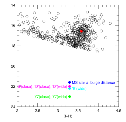
Figure 8: Source locations with respect to the giant clump centroid (red dot) in the $(I-H)/H$ color-magnitude diagram of stars around the source. We mark 4 source locations, where the blue dot represents the location of a late G-type main-sequence star at a bulge distance, the magenta dot denotes the source location with the brightness estimated from ‘Sol B (close)’, ‘Sol D (close)’, and ‘Sol D (wide)’, and the cyan dot is the source location with the source brightness estimated from ‘Sol B (wide)’, and finally the green dot is the source location with the brightness estimated from ‘Sol C (close)’ and ‘Sol C (wide)’.

In Figure 8, we mark the location of the source star with respect to the GC centroid in the $(I-H)/I$ CMD of neighboring stars around the source. We measure the GC centroid $(I-H,I)_{\rm GC}=(3.58,16.57)\pm(0.01,0.07)$, where the errors are derived from the standard error of the mean of clump stars. As is virtually always the case, for each model, the source color is essentially identical $(I-H)_{s}=3.29\pm 0.04$ to much greater precision than the measurement error, which is dominated by the $H$-band photometric errors. Thus $\Delta(I-H)=-0.29\pm 0.04$. Transformation to $(V-I)$ of both the value and error using the color-color relation of Bessell & Brett (1988) yields $\Delta(V-I)=-0.21\pm 0.03$. Based on the well-defined de-reddened color of GC centroid $(V-I)_{0,{\rm GC}}=1.06$ (Bensby et al., 2011), it is estimated that the de-reddened color of the source is

$$(V-I)_{0,s}=(V-I)_{0,{\rm GC}}+\Delta(V-I)=0.85\pm 0.03.$$ (2)

This color corresponds to that of a late G-type main-sequence star with an absolute magnitude of $M_{I,s}\sim 4.9$. From the absolute magnitude of the GC centroid of $M_{I,{\rm GC}}=-0.12$ (Nataf et al., 2013) combined with its apparent brightness $I_{\rm GC}=16.57$ measured on the CMD, then, the apparent magnitude of the source star should be

$$I_{s}=I_{\rm GC}-(M_{I,{\rm GC}}-M_{I,s})\sim 21.6.$$ (3)

3.4 Partial Resolution of Triple-Lens Degeneracy

It is found that the observed light curve can be explained by $(4\times 2=)8$ degenerate triple-lens solutions. In this subsection, we further investigate the individual solutions in order to check the feasibility of resolving the degeneracy among the solutions.

First, we exclude ‘Sol A’ due to its relatively poor fit to the observed light curve compared to the other solutions. From the comparison of $\chi^{2}$ values presented in Table 3, it is found that ‘Sol A’ provides a fit that is poorer than ‘Sol B’, ‘Sol C’, and ‘Sol D’ by $\Delta\chi^{2}=70.7$, 80.7, and 67.5, respectively. These $\chi^{2}$ differences are statistically significant enough to exclude ‘Sol A’.

This leaves three pairs of solutions, one pair for each of ‘Sols B, C, D’. ‘Sol C’ (wide) is favored by $\Delta\chi^{2}=10$ over any other solutions. However, the source position on the CMD is a priori substantially less likely than for ‘Sol B’ and ‘Sol D’. The source brightness determined from the source flux $F_{s}$, presented in Table 3, are $I_{s}=23.00\pm 0.05$ and $22.90\pm 0.02$ for the wide and close solutions, respectively. These are $\gtrsim 1.3$ magnitude fainter than $I_{s}=21.6$, i.e. Eq. (3), estimated based on the relative source position with respect to the GC centroid in the CMD. See Figure 8. To explain such a faint source would require either that the source is very distant (at e.g., $D_{\rm S}\sim 15\,$kpc), or that it is intrinsically dim for its color due to low metallicity (e.g., [Fe/H]$\sim-1.3$). Either of these is possible, although with low probability. For example, Bensby et al. (2017a) find a total of 3 stars with [Fe/H]$<-1.2$ out of their sample of 90 microlensed bulge dwarfs and subgiants. Similarly, Ness et al. (2013) found about 2% of stars with ${\rm[Fe/H]}<-1.2$ in a much larger sample, albeit substantially farther from the Galactic plane than typical microlensing events. Compare Figures 1 and 10 of Bensby et al. (2017b) with Figures 1 and 6 of Ness et al. (2013), respectively. The Bensby et al. (2017a) sample is appropriate for comparison because it faces qualitatively similar selection biases to microlensing surveys that lead to planet detection. On the other hand, Bensby et al. (2017a) found no clear evidence for microlensed sources that lay substantially behind the Galactic bulge.

In brief ‘Sol C’ is mildly favored by $\chi^{2}$ but requires a somewhat unlikely source. If its $\Delta\chi^{2}=10$ advantage could be interpreted at face value according to Gaussian statistics, this solution would be mildly preferred by $\Delta\ln L=\ln(3/90)+10/2=1.6$. However, it is well known that microlensing light curves are affected by subtle systematics at the $\Delta\chi^{2}=$few level, and so cannot be judged according to naive Gaussian statistics. Therefore, we consider that ‘Sol C’ is viable but somewhat disfavored.

On the other hand, ‘Sol B’ and ‘Sol D’ not only provide good fits to the observed light curve but also meet the source brightness constraint. The apparent source magnitudes estimated from $F_{s}$ values of the models are $I_{s}=22.25\pm 0.02$/$22.01\pm 0.04$ for the wide/close solutions of ‘Sol B’ and $I_{s}=21.96\pm 0.02$/$21.96\pm 0.01$ for the wide/close solutions of ‘Sol D’. These are in accordance with $I_{s}\sim 21.6$ estimated from the CMD. We find that the lensing parameters of ‘Sol B’ and ‘Sol D’ models are in the relation of

$$s_{B}\sim{1+q_{B}\over 1-q_{B}\sqrt{1+q_{D}}}s_{D}^{-1},$$ (4)

where $(s_{B},q_{B})$ represent the binary separation and mass ratio of ‘Sol B’ and $(s_{D},q_{D})$ represent those of ‘Sol D’. This indicates that ‘Sol B’ and ‘Sol D’ are the pair of solutions resulting from the well-known close/wide binary-lens degeneracy which is rooted in the symmetry of the lens equation and thus can be severe (Dominik, 1999b; An, 2005). For OGLE-2016-BLG-0613, the degeneracy is quite severe with $\Delta\chi^{2}\lesssim 5$. Note in particular from Figure 5 that the topologies of ‘Sol B’ and ‘Sol D’ are essentially identical and are also distinct from the other three topologies shown.

3.5 Angular Eintein Radius

The angular Einstein radius is estimated from the combination of the normalized source radius $\rho$ and the angular source radius $\theta_{*}$, i.e. $\theta_{\rm E}=\theta_{*}/\rho$. The normalized source radius is measured by analyzing the caustic-crossing part of the light curve where the lensing magnifications are affected by finite-source effects. Although three of the four caustic crossings were covered by either zero or one point (and so yield essentially no information about $\rho$), the planetary-caustic entrance was very well covered by KMTS data. See the lower middle panel of Figure 6.

The angular source radius is estimated based on the de-reddened color and brightness. The de-reddeded $V$-band brightness is estimated by

$$V_{0,s}=I_{0,s}+(V-I)_{0,s},$$ (5)

where $I_{0,s}=I_{{\rm GC},0}-(I_{\rm GC}-I_{s})$, $I_{{\rm GC},0}=14.38$ (Nataf et al., 2013), $I_{\rm GC}=16.57\pm 0.07$, $(V-I)_{0,s}=0.85\pm 0.03$ [Eq. (2)], and $I_{s}$ is given for each solution in Table 3. We convert $(V-I)_{0}$ into $(V-K)_{0}$ using the $VI/VK$ relation of Bessell & Brett (1988). Then, the angular source radius $\theta_{*}$ is determined from the relation between $\theta_{*}$ and $(V,V-K)_{0}$ provided by Kervella et al. (2004).

Table 4: Einstein ring radius and proper motion

Parameters	‘Sol B’		‘Sol C’		‘Sol D’
	Wide	Close	Wide	Close	Wide	Close
$\theta_{\rm E}$ (mas)	$1.20\pm 0.24$	$1.12\pm 0.22$	$1.15\pm 0.22$	$1.15\pm 0.22$	$1.28\pm 0.25$	$1.63\pm 0.32$
$\mu$ (mas yr-1)	$8.50\pm 1.71$	$9.06\pm 1.75$	$5.64\pm 1.11$	$5.86\pm 1.14$	$8.70\pm 1.72$	$11.5\pm 2.20$

Table 5: Physical lens parameters

Parameters	‘Sol B’		‘Sol C’		‘Sol D’
	Wide	Close	Wide	Close	Wide	Close
$D_{\rm L}$ (kpc)	$3.41^{+1.34}_{-1.42}$	$3.56^{+1.30}_{-1.51}$	$3.19^{+1.40}_{-1.27}$	$3.21^{+1.35}_{-1.20}$	$3.84^{+1.44}_{-1.63}$	$2.93^{+1.59}_{-1.44}$
$M_{1}$ ($M_{\odot}$)	$0.72^{+0.55}_{-0.42}$	$0.65^{+0.50}_{-0.37}$	$0.80^{+0.65}_{-0.43}$	$0.81^{+0.64}_{-0.44}$	$0.66^{+0.58}_{-0.38}$	$0.63^{+0.72}_{-0.41}$
$M_{2}$ ($M_{\odot}$)	$0.28^{+0.21}_{-0.16}$	$0.23^{+0.18}_{-0.13}$	$0.023^{+0.019}_{-0.012}$	$0.023^{+0.017}_{-0.012}$	$0.69^{+0.61}_{-0.40}$	$0.70^{+0.80}_{-0.46}$
$M_{3}$ ($M_{J}$)	$4.18^{+3.19}_{-2.43}$	$3.01^{+2.32}_{-1.71}$	$2.74^{+2.23}_{-1.51}$	$2.75^{+2.17}_{-1.49}$	$4.42^{+3.88}_{-2.54}$	$1.17^{+1.33}_{-0.76}$
$a_{\perp,1-2}$ (au)	$2.96^{+1.16}_{-1.23}$	$3.02^{+1.10}_{-1.28}$	$5.00^{+2.19}_{-1.99}$	$5.00^{+2.10}_{-1.87}$	$9.09^{+3.41}_{-3.86}$	$8.66^{+0.42}_{-0.38}$
$a_{\perp,1-3}$ (au)	$6.40^{+2.51}_{-2.63}$	$3.28^{+1.20}_{-1.39}$	$4.19^{+1.84}_{-1.67}$	$3.15^{+1.32}_{-1.18}$	$3.90^{+1.46}_{-1.66}$	$3.04^{+0.15}_{-0.13}$

In Table 4, we present the angular Einstein radii for the viable models ‘Sol B’, ‘Sol C’, and ‘Sol D’. Also presented are the relative lens-source proper motion determined by

$$\mu={\theta_{\rm E}\over t_{\rm E}},\qquad\theta_{\rm E}\equiv\sqrt{\kappa M\pi_{\rm rel}},$$ (6)

where $\pi_{\rm rel}={\rm au}(D_{L}^{-1}-D_{S}^{-1})$ is the lens-source relative parallax and $\kappa\equiv 4G/(c^{2}{\rm au})\simeq 8.14\ {\rm mas}\ M_{\odot}^{-1}$. The inferred angular Einstein radii for the ensemble of solutions are in the range of $1.1\lesssim\theta_{\rm E}/{\rm mas}\lesssim 1.6$. These large values of $\theta_{\rm E}$ virtually rule out bulge lenses and so directly imply that the lens is in the Galactic disk. That is, if we hypothesized that the lens were in the bulge, then (since the bulge is a relatively old population), we could infer $M\lesssim 1.3\,M_{\odot}$. Hence, for $\theta_{\rm E}\gtrsim 1.1\,{\rm mas}$, Equation (6) implies $\pi_{\rm rel}\gtrsim 0.11\,{\rm mas}$, which would contradict the hypothesis that the lens was in the bulge.

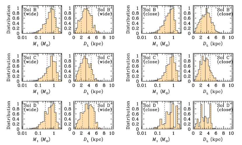
Figure 9: Distributions of the primary mass $M_{1}$ and the distance to the lens $D_{\rm L}$ for the individual solutions obtained from Bayesian analysis. In each panel, the solid vertical line represents the median value and the two dotted lines represent the $1\sigma$ range of the distribution.

3.6 Physical Lens Parameters

For the unique determinations of the lens mass $M$ and distance $D_{\rm L}$, one needs to measure both the angular Einstein radius $\theta_{\rm E}$ and the microlens parallax $\pi_{\rm E}$:

$$M={\theta_{\rm E}\over\kappa\pi_{\rm E}};\qquad D_{\rm L}={{\rm au}\over\pi_{\rm E}\theta_{\rm E}+\pi_{\rm S}},$$ (7)

where $\pi_{\rm S}={\rm au}/D_{S}$ is the source parallax. For OGLE-2016-BLOG-0613, $\theta_{\rm E}$ is measured but $\pi_{\rm E}$ is not measured and thus the values of $M$ and $D_{\rm L}$ cannot be uniquely determined. However, one can still constrain the physical lens parameters based on the measured values of the event time scale $t_{\rm E}$ and the angular Einstein radius $\theta_{\rm E}$.

In order to estimate the mass and distance to the lens, we conduct a Bayesian analysis of the event based on the mass function combined with the models of the physical and dynamical distributions of objects in the Galaxy. We use the initial mass function of Chabrier (2003a) for the mass function of Galactic bulge objects, while we use the present day mass function of Chabrier (2003b) for disk objects. In the mass function, we do not include stellar remnants, i.e. white dwarfs, neutron stars, and black holes, because it would be difficult for planets to survive the AGB/planetary-nebular phase of stellar evolution and no planet belonging to a remnant host is so far known, e.g. Kilic et al. (2009). For the matter distribution, we adopt the Galactic model of Han & Gould (2003). In this model, the matter density distribution is constructed based on a double-exponential disk and a triaxial bulge. We use the dynamical model of Han & Gould (1995) to construct the velocity distribution. In this model, the disk velocity distribution is assumed to be Gaussian about the rotation velocity of the disk and the bulge velocity distribution is modeled to be a triaxial Gaussian with velocity components deduced from the flattening of the bulge via the tensor virial theorem. Based on these models, we generate a large number of artificial lensing events by conducting a Monte Carlo simulation. We then estimate the ranges of $M$ and $D_{\rm L}$ corresponding to the measured event time scale and the angular Einstein radius.

In Table 5, we list the physical parameters of the lens system estimated from the the Bayesian analysis. In Figure 9, we also present the distributions of the primary mass $M_{1}$ and the distance to the lens $D_{\rm L}$ obtained from the Bayesian analysis for the individual solutions. The values denoted by $M_{i}$ represent the masses of the individual lens components, and $a_{\perp,1-2}$ and $a_{\perp,1-3}$ denote the projected $M_{1}-M_{2}$ and $M_{1}-M_{3}$ separations, respectively. We note that the unit of $M_{1}$ and $M_{2}$ is the solar mass, $M_{\odot}$, while the unit of $M_{3}$ is the Jupiter mass, $M_{J}$. The presented physical parameters are the median values of the corresponding distributions and the uncertainties are estimated as the standard deviations of the distributions.

All three pairs of solutions shown in Table 5 are comprised of a super-Jupiter planet in a binary-star system, whose primary is a K dwarf. They are all located in the Galactic disk, about half-way toward the bulge. The major difference among these solutions is that for ‘Sol B’ and ‘Sol D’, the components of the binary are of equal (B) or comparable (D) mass, whereas for ‘Sol C’, the second component of the binary is a low-mass brown dwarf. We note that in all cases, the projected separations of the secondary and the planet are roughly comparable, so that if the system lay in the plane of the sky it would be unstable. This is a result of a generic selection bias of microlensing. Binary lenses, and in particular planets, are most easily discovered if they lie separated in projection by roughly one Einstein radius. See e.g., Figure 7 of Mróz et al. (2017). This bias affects multi-lens systems by the square. OGLE-2012-BLG-0026 (Han et al., 2013) provides an excellent example of such bias. Hence, stable, hierarchical systems are preferentially seen at an angle such that the projected separations are comparable.

4 Discussion

OGLE-2016-BLG-0613 is of scientific importance because it demonstrates that planets in binary systems can be readily detected using the microlensing method. The planet is the fourth microlensing planet in binary systems followed by OGLE-2008-BLG-092L (Poleski et al., 2014), OGLE-2013-BLG-0341L (Gould et al., 2014), and OGLE-2007-BLG-349 (Bennett et al., 2016). Since the region of planet sensitivity is different from those of other planet-detection methods, the microlensing method will enrich the sample of planets in binaries, helping us to understand details about the formation mechanism of these planets.

The event illustrates the difficulty of 3-body lensing modeling. As shown in the previous section, interpreting the light curve suffers from multifold degeneracy due to the complexity of triple-lens topology combined with insufficient data quality. Such a difficulty in the interpretation was found in the case of another triple-lens event OGLE-2007-BLG-349 for which there existed two possible interpretations of the circumbinary-planet model and two-planet model. Bennett et al. (2016) were able to resolve the degeneracy with additional high-resolution images obtained from Hubble Space Telescope observations.

‘Sol C’ (star + brown-dwarf + super-Jupiter) represents a substantially different type of system from either ‘Sol B’ or ‘Sol D’ (comparable mass binary with super-Jupiter). It would therefore be of considerable interest to distinguish between these two classes. This will be quite straightforward once the source and lens are sufficiently separated to be resolved in high-resolution images (whether from space or the ground) because ‘Sol C’ has both a much lower proper motion (Table 4) and a much fainter source star (Figure 8). In fact, even if ‘Sol C’ is the correct solution, it is only necessary to wait until the lens and source would be separately resolved in ‘Sol B’ and ‘Sol D’, based on their substantially larger proper motions. In that case, if the lens and source are not separately resolved, this non-detection would demonstrate that ‘Sol C’ was correct. We note that for the case of OGLE-2005-BLG-169, which had a similar proper motions to ‘Sol B’ and ‘Sol D’, Batista et al. (2015) clearly resolved the source and lens with Keck adaptive optics observations taken 8.2 years later, while Bennett et al. (2015) marginally resolved them after 6.5 years using the Hubble Space Telescope. In principle, it is also possible to both detect the lens and measure its proper motion by subtracting out the source light from high-resolution images. This may be possible in the present case. However, application of this approach would be significantly complicated by the existence of several different solutions with very different source fluxes.

5 Conclusion

We analyzed the microlensing event OGLE-2016-BLG-0613 for which the light curve appeared to be that of a typical binary-lens event with two caustic spikes but with a short-term discontinuous feature on the smooth trough region between the spikes. It was found that the overall feature of the light curve was described by multiple binary-lens solutions but the short-term discontinuous feature could be explained by none of these solutions. We found that the discontinuous feature could be explained by introducing a low-mass planetary companion to the binary lens. We found 4 degenerate triple-lens solutions, among which one was excluded due to the relatively poor fit compared to the other solutions. For each of the remaining three classes of solutions, there is a pair of sub-solutions according to the well-known close-wide degeneracy for planets. In two of the three classes of solutions, the two binary components are of comparable mass, while in the third, the second component of the binary is a low mass brown dwarf. The degeneracy between the binary-star/planet lens model(s) and the star/brown-dwarf/planet lens model can be resolved by future high-resolution imaging observation.

References

- Abt (1983) Abt, H. A. 1983, ARA&A, 21, 343
- Alard & Lupton (1998) Alard, C., & Lupton, R. H. 1998, ApJ, 503, 325
- Albrow et al. (2002) Albrow, M. D., An, J., Beaulieu, J.-P., et al. 2002 ApJ, 572, 1031
- Albrow et al. (2000) Albrow, M. D., Beaulieu, J.-P., Caldwell, J. A. R., et al. 2000, ApJ, 534, 894
- Albrow et al. (2009) Albrow, M. D., Horne, K., Bramich, D. M., et al. 2009, MNRAS, 397, 2099
- An (2005) An, J. H. 2005, MNRAS, 356, 1409
- Batista et al. (2015) Batista, V., Beaulieu, J.-P., Bennett, D. P., et al. 2015, ApJ, 808, 170
- Beaulieu et al. (2016) Beaulieu, J.-P., Bennett, D. P., Batista, V., et al. 2016, ApJ, 824, 83
- Bennett et al. (2015) Bennett, D. P., Bhattacharya, A., Anderson, J., et al. 2015, ApJ, 808, 169
- Bennett et al. (1999) Bennett, D. P., Rhie, S. H., Becker, A. C., et al. 1999, Nature, 402, 57
- Bennett et al. (2010) Bennett, D. P., Rhie, S. H., Nikolaev, S., et al. 2010, ApJ, 713, 837
- Bennett et al. (2016) Bennett, D. P., Rhie, S. H., Udalski, A., et al. 2016, AJ, 152, 125
- Bensby et al. (2011) Bensby, T., Adén, D., Melńdez, J., et al. 2011, A&A, 533, A134
- Bensby et al. (2017a) Bensby, T., Feltzing, S., Gould, A., et al. 2017a, A&A, submitted, arXiv:1702:02971
- Bensby et al. (2017b) Bensby, T., Feltzing, S., Gould, A., Tee. J. C., Johnson, J. A., Asplund, M., Meléndez, J., Lucatello, S., Howes, M. 2017, Discovery of Galaxy, Proceedings IAU Symposium, in press, arXiv:1707:05960
- Bessell & Brett (1988) Bessell, M. S., & Brett, J. M. 1988, PASP, 100, 1134
- Boss (2006) Boss, A. P. 2006, ApJ, 643, 501
- Bozza (1999) Bozza V. 1999, A&A, 348, 311
- Bozza et al. (2016) Bozza, V., Shvartzvald, Y., Udalski, A., et al. 2016, ApJ, 820, 70
- Chabrier (2003a) Chabrier, G. 2003a, PASP, 115, 763
- Chabrier (2003b) Chabrier, G. 2003b, ApJ, 586, L133
- Choi et al. (2012) Choi, J.-Y., Shin, I.-G., Han, C., et al. 2012, ApJ, 756, 48
- Danék & Heyrovský (2015) Danék, K., & Heyrovský, D. 2015, ApJ, .806, 99
- Dominik (1999a) Dominik, M. 1999a, A&A, 349, 108
- Dominik (1999b) Dominik, M. 1999b, A&A, 341, 943
- Gaudi et al. (2008) Gaudi, B. S., Bennett, D. P., Udalski, A., et al. 2008, Science, 319 927
- Gaudi et al. (1998) Gaudi, B. S., Naber, R. M., & Sackett, P. D. 1998, ApJ, 502, L33
- Gould (1992) Gould, A. 1992, ApJ, 392, 442
- Gould (1994) Gould, A. 1992, ApJ, 421, L75
- Gould (2008) Gould, A. 2008, ApJ, 681, 1593
- Gould & Loeb (1992) Gould, A., & Loeb, A. 1992, ApJ, 396, 104
- Gould et al. (2014) Gould, A., Udalski, A., Shin, I.-G., et al. 2014, Science, 345, 46
- Griest & Safizadeh (1998) Griest, K ., & Safizadeh, N. 1998, ApJ, 500, 37
- Han (2005) Han, C. 2005, ApJ, 629, 1102
- Han (2008) Han, C. 2008, ApJ, 676, L53
- Han & Gould (1995) Han, C., & Gould, A. 1995, ApJ, 447, 53
- Han & Gould (2003) Han, C., & Gould, A. 2003, ApJ, 592, 172
- Han et al. (2016) Han, C., Bennett, D. P., Udalski, A., & Jung, Y. K. 2016, ApJ, 825, 8
- Han et al. (2013) Han, C., Udalski, A., Choi, J.-Y., et al. 2013, ApJ, 762, L28
- Henderson, et al. (2016) Henderson, C. B., Poleski, R., Penny, M. 2016, PASP, 128, 4401
- Horch et al. (2014) Horch, E. P., Howell, S. B., Everett, M. E., & Ciardi, D. R. 2014, ApJ, 795, 60
- Ida & Lin (2004) Ida, S., & Lin, D. N. C. 2004, ApJ, 616, 567
- Jung et al. (2013) Jung, Y. K., Han, C., Gould, A., & Maoz, D. 2013, ApJ, 768, L7
- Kervella et al. (2004) Kervella, P., Thévenin, F., Di Folco, E., & Ségransan, D. 2004, A&A, 426, 297
- Kilic et al. (2009) Kilic, M., Gould, A., & Koester, D. 2009, ApJ, 705, 1219
- Kim et al. (2016) Kim, S.-L., Lee, C.-U., Park, B.-G., et al. 2016, JKAS, 49, 37
- Lee et al. (2008) Lee, D.-W., Lee, C.-U., Park, B.-G., Chung, S.-J., Kim, H.-I., Kim, Y.-S., & Han, C. 2008, ApJ, 672, L623
- Luhn et al. (2016) Luhn, J. K., Penny, M. T., & Gaudi, B. S. 2016, ApJ, 827, L61
- Mao & Paczyński (1991) Mao, S., & Paczyński, B. 1991, ApJ, 374, L37
- Mróz et al. (2017) Mróz, P., Han, C., Udalski, A., et al. 2017, AJ, 153, 143
- Nataf et al. (2013) Nataf, D. M., Gould, A., Fouqué, P., et al. 2013, ApJ, 769, 88
- Ness et al. (2013) Ness, M., Freeman, K., Athanassoula, E., et al. 2013, MNRAS, 430, 836
- Pejcha & Heyrovský (2009) Pejcha, O., & Heyrovský, D. 2009, ApJ, 690, 1772
- Petters et al. (2001) Petters A. O., Levine H., & Wambsganss J., 2001, Singularity Theory and Gravitational Lensing, 1st edn. (Basel: Birkhäuser)
- Poleski et al. (2014) Poleski, R., Skowron, J., Udalski, A., et al. 2014, ApJ, 795, 42
- Refsdal (1966) Refsdal, S. 1966, MNRAS, 134, 315
- Ryu et al. (2017) Ryu, Y.-H., Yee, J. C., Udalski, A., et al. 2017, AAS journals, submitted.
- Schneider et al. (1992) Schneider P., Ehlers J., & Falco E. E., 1992, Gravitational Lenses, 1st edn. (New York: Springer-Verlag)
- Schneider & Weiss (1986) Schneider, P., & Weiss, A. 1986, A&A, 164, 237
- Shvartzvald et al. (2017) Shvartzvald, Y., Bryden, G., Gould, A., Henderson, C. B., Howell, S. B., & Beichman, C. 2017, AJ, 153, 61
- Song et al. (2014) Song, Y.-Y., Mao, S., & An, J. H. 2014, MNRAS, 437, 4006
- Thebault & Haghighipour (2015) Thebault, P., & Haghighipour, N. 2015, Planetary Exploration and Science: Recent Results and Advances, eds. S. Jin, N. Haghighipour, W-H. Ip (Berlin: Springer), 309
- Udalski (2003) Udalski, A. 2003, Acta Astron., 53, 291
- Udalski et al. (2015) Udalski, A., Jung, Y. K., Han, C., et al. 2015, ApJ, 812, 47
- Udalski et al. (2015) Udalski, A., Yee, J. C., Gould, A., et al. 2015, ApJ, 799, 237
- Yee et al. (2012) Yee, J. C., Shvartzvald, Y., Gal-Yam, A., et al. 2012, ApJ, 755, 102
- Yoo et al. (2004) Yoo, J., DePoy, D. L., Gal-Yam, A., et al. 2004, ApJ, 603, 139