Robust Online Regression in Cautious Consolidation

Online Robust Regression via Cautious Robust Consolidation

Online Robust Regression under Heterogeneously Distributed Corruption

Scalable Robust Regression under Arbitrarily Distributed Data Corruption

Online Robust Regression under Arbitrarily Distributed Data Corruption

Online Robust Regression under Adversary
Data Corruption

Online and Distributed Robust Regressions
under Adversarial Data Corruption

Abstract

In today’s era of big data, robust least-squares regression becomes a more challenging problem when considering the adversarial corruption along with explosive growth of datasets. Traditional robust methods can handle the noise but suffer from several challenges when applied in huge dataset including 1) computational infeasibility of handling an entire dataset at once, 2) existence of heterogeneously distributed corruption, and 3) difficulty in corruption estimation when data cannot be entirely loaded. This paper proposes online and distributed robust regression approaches, both of which can concurrently address all the above challenges. Specifically, the distributed algorithm optimizes the regression coefficients of each data block via heuristic hard thresholding and combines all the estimates in a distributed robust consolidation. Furthermore, an online version of the distributed algorithm is proposed to incrementally update the existing estimates with new incoming data. We also prove that our algorithms benefit from strong robustness guarantees in terms of regression coefficient recovery with a constant upper bound on the error of state-of-the-art batch methods. Extensive experiments on synthetic and real datasets demonstrate that our approaches are superior to those of existing methods in effectiveness, with competitive efficiency.

1 Introduction

In the era of data explosion, the fast-growing amount of data makes processing entire datasets at once remarkably difficult. For instance, urban Internet of Things (IoT) systems [1] can produce millions of data records every second in monitoring air quality, energy consumption, and traffic congestion. More challenging, the presence of noise and corruption in real-world data can be inevitably caused by accidental outliers [2], transmission loss [3], or even adversarial data attacks [4]. As the most popular statistical approach, the traditional least-squares regression method is vulnerable to outlier observations [5] and not scalable to large datasets [6]. By considering both robustness and scalability in a least-squares regression model, we study scalable robust least-squares regression (SRLR) to handle the problem of learning a reliable set of regression coefficients given a large dataset with several adversarial corruptions in its response vector. A commonly adopted model from existing robust regression methods [7][8] assumes that the observed response is obtained from the generative model $\bm{y}=X^{T}\bm{\beta}_{*}+\bm{u}$, where $\bm{\beta}_{*}$ is the true regression coefficients that we wish to recover and $\bm{u}$ is the corruption vector with arbitrary values. However, in the SRLR problem, our goal is to recover the true regression coefficients under the assumption that both the observed response $\bm{y}$ and data matrix $X$ are too large to be loaded into a single machine. Due to the ubiquitousness of data corruptions and explosive data growth, SRLR has become a critical component of several important real-world applications in various domains such as economics [9], signal processing [10], and image processing [11].

Existing robust learning methods typically focus on modeling the entire dataset at once; however, they may meet the bottleneck in terms of computation and memory as more and more datasets are becoming too large to be handled integrally. For those seeking to address this issue, the major challenges can be summarized as follows. 1) Computational infeasibility of handling the entire dataset at once. Existing robust methods typically generate the predictor by learning on the entire training dataset. However, the explosive growth of data makes it infeasible to handle the entire dataset up to a terabyte or even petabyte at once. Therefore, a scalable algorithm is required to handle the robust regression task for massive datasets. 2) Existence of heterogeneously distributed corruption. Due to the unpredictability of corruptions, the corrupted samples can be arbitrarily distributed in the whole dataset. Considering the entire dataset as the combination of multiple mini-batches, some batches may contain large amounts of outliers. Thus, simply applying the robust method on each batch and averaging all the estimates together is not an ideal strategy, as some estimates will be arbitrarily poor and break down the overall performance of robustness. 3) Difficulty in corruption estimation when data cannot be entirely loaded. Most robust methods assume the corruption ratio of input data is a known parameter; however, if a small batch of data can be loaded as inputs for robust methods, it is infeasible to know the corruption ratio of all the mini-batches. Moreover, simply using a unified corruption ratio for all the mini-batches is clearly not an ideal solution as corrupted samples can be regarded as uncorrupted, and vice versa. In addition, even though some robust methods can estimate the corruption ratio based on data observations, it is also infeasible to estimate the ratio when corruption in one mini-batch is greater than 50%. However, the situation can be very common when corruption is heterogeneously distributed.

In order to simultaneously address all these technical challenges, this paper presents a novel Distributed Robust Least-squares Regression (DRLR) method and its online version, named Online Roubst Least-squares Regression (ORLR) to handle the scalable robust regression problem in large datasets with adversarial corruption. In DRLR, the regression coefficient of each mini-batch is optimized via heuristic hard thresholding, and then all the estimates are combined in distributed robust consolidation. Based on DRLR, the ORLR algorithm incrementally updates the existing estimates by replacing old corrupted estimates with those of new incoming data, which is more efficient than DRLR in handling new data and reflects the time-varying characteristics. Also, we prove that both DRLR and ORLR preserve the overall robustness of regression coefficients in the entire dataset. The main contributions of this paper are as follows:

• Formulating a framework for the SRLR problem. A framework is proposed for scalable robust least-squares regression problem where the entire data with adversarial corruption is too large to store in memory all at once. Specifically, given a large dataset with adversarial corruptions, a reliable set of regression coefficients is learned with limited memory.

• Proposing online and distributed algorithms to handle the adversarial corruption. By utilizing robust consolidation methods, we propose both online and distributed algorithms to obtain overall robustness even though the corruption is arbitrarily distributed. Moreover, the online algorithm performs more efficiently in handling new incoming data and presents the time-varying characteristics of regression coefficients.

• Providing a rigorous robustness guarantee for regression coefficient recovery. We prove that our online and distributed algorithms recover the true regression coefficient with a constant upper bound on the error of state-of-the-art batch methods under the assumption that corruption can be heterogeneously distributed. Specifically, the upper bound of online algorithm will be infinitely close to distributed algorithm when the number of mini-batches is large enough.

• Conducting extensive experiments for performance evaluations. The proposed method was evaluated on both synthetic data and real-world datasets with various corruption and data-size settings. The results demonstrate that the proposed approaches consistently outperform existing methods along multiple metrics with a competitive running time.

The rest of this paper is organized as follows. Section 2 reviews background and related work, and Section 3 introduces the problem setup. The proposed online and distributed robust regression algorithms are presented in Section 4. Section 5 presents the proof of recovery guarantee in regression coefficients. The experiments on both synthetic and real-world datasets are presented in Section 6, and the paper concludes with a summary of the research in Section 7.

2 Related Work

The work related to this paper is summarized in two categories below.

Robust regression model: A large body of literature on the robust regression problem has been built over the last few decades. Most of studies focus on handling stochastic noise or small bounded noise [12][13][14], but these methods, modeling the corruption on stochastic distributions, cannot be applied to data that may exhibit malicious corruption [4]. Some studies assume the adversarial corruption in the data, but most of them lack the strong guarantee of regression coefficients recovery under the arbitrary corruption assumption [4][6]. Chen et al. [4] proposed a robust algorithm based on a trimmed inner product, but the recovery boundary is not tight to ground truth in a massive dataset. McWilliams et al. [6] proposed a sub-sampling algorithm for large-scale corrupted linear regression, but their recovery result is not close to an exact recovery [7]. To pursue exact recovery results for robust regression problem, some studies focused on $L_{1}$ penalty based convex formulations [15][16]. However, these methods imposed severe restrictions on the data distribution such as row-sampling from an incoherent orthogonal matrix[16].

Currently, most research in this area requires the corruption ratio parameter, which is difficult to determine under the assumption that the dataset can be arbitrarily corrupted. For instance, She and Owen [17] rely on a regularization parameter to control the size of the uncorrupted set based on soft-thresholding. Instead of a regularization parameter, Chen et al. [18] require the upper bound of the outliers number, which is also difficult to estimate. Bhatia et al. [7] proposed a hard-thesholding algorithm with a strong guarantee of coefficient recovery under a mild assumption on input data. However, its recovery error can be more than doubled in size if the corruption ratio is far from the true value. Recently, Zhang et al. [8] proposed a robust algorithm that learns the optimal uncorrupted set via a heuristic method. However, all of these approaches require the entire training dataset to be loaded and learned at once, which is infeasible to apply in massive and fast growing data.

Online and distributed learning: Most of the existing online learning methods optimize surrogate functions such as stochastic gradient descent [19][20] to update estimates incrementally. For instance, Duchi et al. [19] proposed a new, informative subgradient method that dynamically incorporates the geometric knowledge of the data observed in earlier iterations. Some adaptive linear regression methods such as recursive least squares [21] and online passive aggressive algorithms [22] provide an incremental update on the regression model for new data to capture time-varying characteristics. However, these methods cannot handle the outlier samples in the streaming data. For distributed learning [23][24], most approaches such as MapReduce [25] focus on distributed solutions for large-scale problems that are not robust to noise and corruption in real-world data.

The existing distributed robust optimization methods can be divided into two categories: those that use moment information [26][27] and those that utilize directly on the probability distributions [28][29][30]. For instance, Delage et al. [31] proposed a model that describes uncertainty in both the distribution form and moments in a distributed robust stochastic program. However, these methods assume either the moment information or probability distribution as prior knowledge, which is difficult to know in practice. In robust online learning, few methods have been proposed in the past few years. For instance, Sharma et al. [32] proposed an online smoothed passive-aggressive algorithm to update estimates incrementally in a robust manner. However, the method assumes the corruption is in stochastic distributions, which is infeasible for data with adversarial corruption. Recently, Feng et al. [33] proposed an online robust learning approach that gives a provable robustness guarantee under the assumption that data corruption is heterogeneously distributed. However, the method requires that the corruption ratio of each data batch be given as parameters, which is not practical for users to estimate.

3 Problem Formulation

In this section, the problem addressed by this research is formulated.

In the setting of online and distributed learning, we consider the samples to be provided in a sequence of mini batches as $\{X^{(1)},\dots,X^{(m)}\}$, where $X^{(i)}\in\mathbbm{R}^{p\times n}$ represents the sample data for the $i\textsuperscript{th}$ batch. We assume the corresponding response vector $\bm{y}^{(i)}\in\mathbbm{R}^{n\times 1}$ is generated using the following model:

$$\bm{y}^{(i)}={\big{[}\bm{X}^{(i)}\big{]}}^{T}\bm{\beta}_{*}+\bm{u}^{(i)}+\bm{\varepsilon}^{(i)}$$ (1)

where $\bm{\beta}_{*}\in\mathbbm{R}^{p\times 1}$ is the ground truth coefficients of the regression model and $\bm{u}^{(i)}$ is the adversarial corruption vector of the $i\textsuperscript{th}$ mini-batch. $\bm{\varepsilon}^{(i)}$ represents the additive dense noise for the $i\textsuperscript{th}$ mini batch, where $\varepsilon_{j}^{(i)}\sim\mathcal{N}(0,\sigma^{2})$. The notations used in this paper are summarized in Table 1.

The goal of addressing our problem is to recover the regression coefficients $\hat{\bm{\beta}}$ and determine the uncorrupted set $\hat{S}$ for the entire dataset. The problem is formally defined as follows:

$$\hat{\bm{\beta}},\hat{S}= \operatorname*{arg\,min}_{\bm{\beta},S}\big{\|}\bm{y}_{S}-X_{S}^{T}\bm{\beta}\big{\|}_{2}^{2}$$ (2)

$$s.t.\ \ \ S\in\big{\{}\Omega\big{(}Z\big{)} \big{|}\ \forall i\leq m,\forall j\leq\lvert Z^{(i)}\rvert:Z_{j}^{(i)}\geq h(\bm{r}^{(i)})\big{\}}$$

We define $Z^{(i)}$ as the estimated uncorrupted set for the $i\textsuperscript{th}$ mini-batch and $Z=\{Z^{(1)},...\ ,Z^{(m)}\}$ as the collection of uncorrupted sets for all the mini-batches. The size of set $Z^{(i)}$ is represented as $\lvert Z^{(i)}\rvert$. The function $\Omega(\cdot)$ consolidates the estimates of all the mini-batches in terms of the distributed or online setting. $\bm{y}_{S}$ restricts the row of $\bm{y}$ to indices in $S$, and $X_{S}$ signifies that the columns of $X$ are restricted to indices in $S$. Therefore, we have $\bm{y}_{S}\in\mathbbm{R}^{|S|\times 1}$ and $X_{S}\in\mathbbm{R}^{p\times|S|}$, where $p$ is the number of features and $|S|$ is the size of the uncorrupted set $S\subset[m\cdot n]$. The notation $Z^{(i)}_{*}=\overline{supp(\bm{u}^{(i)})}$ represents the true set of uncorrupted points in the $i\textsuperscript{th}$ mini-batch. Also, the residual vector $\bm{r}^{(i)}\in\mathbbm{R}^{n}$ of the $i\textsuperscript{th}$ mini-batch is defined as $\bm{r}^{(i)}=\bm{y}^{(i)}-{\big{[}X^{(i)}\big{]}}^{T}\bm{\beta}$. Specifically, we use the notation $\bm{r}^{(i)}_{Z}$ to represent the $|Z^{(i)}|$-dimensional residual vector containing the components in $Z^{(i)}$. The constraint of $Z^{(i)}$ is determined by function $h(\cdot)$, which is designed to estimate the size of the uncorrupted set of each mini-batch according to the residual vector $\bm{r}^{(i)}$. The uncorrupted set of each mini-batch will be consolidated by function $\Omega(\cdot)$ in both online and distributed approaches. The details of the heuristic function $h(\cdot)$ and consolidation function $\Omega(\cdot)$ will be explained in Section 4.

Table 1: Math Notations

Notations	Explanations
$X^{(i)}\in\mathbbm{R}^{p\times n}$	collection of data samples of the $i\textsuperscript{th}$ mini-batch
$\bm{y}^{(i)}\in\mathbbm{R}^{n\times 1}$	response vector of the $i\textsuperscript{th}$ mini-batch
$\bm{\beta}^{(i)}\in\mathbbm{R}^{p\times 1}$	estimated regression coefficient of the $i\textsuperscript{th}$ batch
$\bm{\beta}^{(i)}_{*}\in\mathbbm{R}^{p\times 1}$	ground truth regression coefficient of the $i\textsuperscript{th}$ batch
$\bm{u}^{(i)}\in\mathbbm{R}^{n\times 1}$	corruption vector of the $i\textsuperscript{th}$ batch
$\bm{r}^{(i)}\in\mathbbm{R}^{n\times 1}$	residual vector of the $i\textsuperscript{th}$ batch
$\bm{\varepsilon}^{(i)}\in\mathbbm{R}^{n\times 1}$	dense noise vector of the $i\textsuperscript{th}$ batch
$Z^{(i)}\subseteq[n]$	estimated uncorrupted set of the $i\textsuperscript{th}$ batch
$Z^{(i)}_{*}\subseteq[n]$	ground truth uncorrupted set, where $Z^{(i)}_{*}=\overline{supp(\bm{u}^{(i)})}$
$S\subseteq[m\cdot n]$	estimated uncorrupted set of entire dataset

The problem defined above is very challenging in the following three aspects. First, the least-squares function can be naively solved by taking the derivative to zero. However, as the data samples of all $m$ mini-batches are too large to be loaded into memory simultaneously, it is impossible to calculate $\bm{\beta}$ from all the batches directly by this method. Moreover, based on the fact that the corruption ratio can be varied for each mini-batch, we cannot simply estimate the corruption set by using a fixed ratio for each mini-batch. In addition, since corruption is not uniformly distributed, some mini-batches may contain an overwhelmingly amount of corrupted samples. The corresponding estimates of regression coefficients can be arbitrarily poor and break down the overall result. In the next section, we present both online and distributed robust regression algorithms based on heuristic hard thresholding and robust consolidation to address all three challenges.

4 Methodology

In this section, we propose both online and distributed robust regression algorithms to handle large datasets in multiple mini-batches. To handle each single mini-batch among these mini-batches, a heuristic robust regression method (HRR) is proposed in Section 4.1. Based on HRR, a new approach, DRLR, is presented in Section 4.2 to process multiple mini-batches in distributed manner. Furthermore, in Section 4.3, a novel online version of DRLR, namely ORLR, is proposed to incrementally update the estimate of regression coefficients with new incoming data.

4.1 Single-Batch Heuristic Robust Regression

In order to efficiently solve the single batch problem when $m$ = $1$ in Equation (2), we propose a robust regression algorithm, HRR, based on heuristic hard thresholding. The algorithm heuristically determines the uncorrupted set $Z^{(i)}$ for the $i\textsuperscript{th}$ mini-batch according to its residual vector $\bm{r}^{(i)}$. Specifically, a novel heuristic function $h(\cdot)$ is proposed to estimate the lower-bound size of the uncorrupted set $Z^{(i)}$ for each mini batch, which is formally defined as

$$h(\bm{r}^{(i)}):= \operatorname*{arg\,max}_{\tau\in\mathbbm{Z}^{+},\tau\leq n}\tau\ \ \ \ s.t.\ \ r^{(i)}_{\varphi(\tau)}\leq\frac{2\tau r^{(i)}_{\varphi(\tau_{o})}}{\tau_{o}}$$ (3)

where the residual vector of $i\textsuperscript{th}$ mini-batch is denoted by $\bm{r}^{(i)}=\bm{y}^{(i)}-{\big{[}X^{(i)}\big{]}}^{T}\bm{\beta}^{(i)}$, and $r^{(i)}_{\varphi(k)}$ represents the $k\textsuperscript{th}$ elements of $\bm{r}^{(i)}$ in ascending order of magnitude. The variable $\tau_{o}$ in the constraint is defined as

$$\tau_{o} =\operatorname*{arg\,min}_{\left\lceil n/2\right\rceil\leq\tau\leq n}\ \left\lvert{\Big{(}r^{(i)}_{\varphi(\tau)}\Big{)}}^{2}-\frac{\lVert\bm{r}^{(i)}_{Z_{\tau^{\prime}}}\rVert_{2}^{2}}{\tau^{\prime}}\ \ \right\rvert$$ (4)

where $\tau^{\prime}=\tau-\left\lceil n/2\right\rceil$ and $Z_{\tau^{\prime}}$ is the position set containing the smallest $\tau^{\prime}$ elements in residual $\bm{r}^{(i)}$.

The design of the heuristic estimator follows a natural intuition that data points with unbounded corruption always have a residual higher in magnitude than that of uncorrupted data. Moreover, the constraint in Equation (3) ensures the residual of the largest element $\tau$ in our estimation cannot be too much larger than the residual of a smaller element $\tau_{o}$. If the element $\tau_{o}$ is too small, some uncorrupted elements will be excluded from our estimation, but if the element is too large, some corrupted elements will be included. The formal definition of $\tau_{o}$ is shown in Equation (4), in which $\tau_{o}$ is defined as a value whose squared residual is closest to ${\lVert\bm{r}^{(i)}_{Z_{\tau^{\prime}}}\rVert_{2}^{2}}/{\tau^{\prime}}$, where $\tau^{\prime}$ is less than the ground truth threshold $\tau_{*}$. This design ensures that $\lvert Z^{(i)}_{*}\cap Z^{(i)}_{t}\rvert\geq\tau-n/2$, which means at least $\tau-n/2$ elements are correctly estimated in $Z^{(i)}_{t}$. In addition, the precision of the estimated uncorrupted set can be easily achieved when fewer elements are included in the estimation, but with low recall value. To increase the recall of our estimation, the objective function in Equation (3) chooses the maximum uncorrupted set size.

Input: Corrupted data samples $X\in\mathbbm{R}^{p\times n}$ and response vector $\bm{y}\in\mathbbm{R}^{n\times 1}$ for single mini batch, tolerance $\epsilon$

Output: solution $\hat{\bm{\beta}}$, $\hat{Z}$

1 $Z_{0}$ = [n], $t$ $\leftarrow$ 0

2 repeat

3       $\bm{\beta}^{t+1}\leftarrow(X_{Z_{t}}X_{Z_{t}}^{T})^{-1}X_{Z_{t}}\bm{y}_{Z_{t}}$

4       $\bm{r}^{t+1}\leftarrow|\bm{y}-X^{T}\bm{\beta}^{t+1}|$

5       $Z_{t+1}\leftarrow$ $\mathcal{H}(\bm{r}^{t+1})$, where $\mathcal{H}(\cdot)$ is defined in Equation (5).

6       $t\leftarrow t+1$

7      

8until $\|\bm{r}_{Z_{t+1}}^{t+1}-\bm{r}_{Z_{t}}^{t}\|_{2}<\epsilon n$

return $\bm{\beta}^{t+1}$, $Z_{t+1}$

Algorithm 1 Hrr Algorithm

Applying the uncorrupted set size generated by $h(\cdot)$, the heuristic hard thresholding is defined as follows:

Definition 1 (Heuristic Hard Thresholding).

Defining $\varphi^{-1}_{\bm{r}}(i)$ as the position of the $i$^th element in residual vector $\bm{r}$’s ascending order of magnitude, the heuristic hard thresholding of $\bm{r}$ is defined as

$$\mathcal{H}(\bm{r})=\{i\in[n]:\varphi^{-1}_{\bm{r}}(i)\leq h(\bm{r})\}$$ (5)

The optimization of $Z^{(i)}$ is formulated as solving Equation (5), where the set returned by $\mathcal{H}(\bm{r}^{(i)})$ will be used to determine regression coefficients $\bm{\beta}^{(i)}$.

The details of the HRR algorithm are shown in Algorithm 1, which follows an intuitive strategy of updating regression coefficient $\bm{\beta}^{(i)}$ to provide a better fit for the current estimated uncorrupted set $Z_{t}$ in Line 3, and updating the residual vector in Line 4. It then estimates the uncorrupted set $Z_{t+1}$ via heuristic hard thresholding in Line 5 based on residual vector $\bm{r}$ in the current iteration. The algorithm continues until the change in the residual vector falls within a small range.

4.2 Distributed Robust Regression

Given data samples $\{(X^{(1)},\bm{y}^{(1)}),\dots,(X^{(m)},\bm{y}^{(m)})\}$ in a sequence of mini-batches, a distributed robust regression algorithm, named DRLR, is proposed to optimize the robust regression coefficients in distributed approach without loading entire data at one time. Before we dive into the details of the DRLR algorithm, we provide some key definitions.

Definition 2 (Estimate Distance).

Defining $\bm{\beta}^{(i)}$ and $\bm{\beta}^{(j)}$ as the estimate of the regression coefficients for the $i\textsuperscript{th}$ and $j\textsuperscript{th}$ mini-batches respectively, the distance between the two estimates is defined as

$$d_{i,j}=\lVert\bm{\beta}^{(i)}-\bm{\beta}^{(j)}\rVert_{2}$$ (6)

Based on the definition of estimate distance, we define the distance vector of the $i\textsuperscript{th}$ mini-batch as $\bm{d}^{(i)}\in\mathbbm{R}^{m\times 1}$, where $m$ is the total number of batches and $\bm{d}_{j}^{(i)}$ represents the distance from the estimate of the $i\textsuperscript{th}$ batch to the $j\textsuperscript{th}$ batch ($1\leq j\leq m$). We also define $\sigma_{k}(\bm{d}^{(i)})$ and $\delta_{k}(\bm{d}^{(i)})$ as the value and index of the $k\textsuperscript{th}$ smallest value in distance vector $\bm{d}^{(i)}$, respectively. For instance, if the $3\textsuperscript{rd}$ batch is the $5\textsuperscript{th}$ smallest distance in $\bm{d}^{(i)}$ with $d_{3}^{(i)}=0.3$, then we have $\sigma_{5}(\bm{d}^{(i)})=0.3$ and $\delta_{5}(\bm{d}^{(i)})=3$.

Definition 3 (Pivot Batch).

Given a set of mini-batch estimates $\{\bm{\beta}^{(1)},\dots,\bm{\beta}^{(m)}\}$ and defining $\bm{d}^{(i)}$ as the distance vector of the $i\textsuperscript{th}$ batch, the $p\textsuperscript{th}$ batch is defined as pivot batch if it satisfies

$$p=\operatorname*{arg\,min}_{i}\sigma_{\tilde{m}}(\bm{d}^{(i)})$$ (7)

where $\tilde{m}=\lfloor m/2\rfloor+1$ is the upper number of half batches. By using the definition of pivot batch, we define the dominating set as follows.

Definition 4 (Dominating Set).

Given a set of mini-batch estimates $\{\bm{\beta}^{(1)},\dots,\bm{\beta}^{(m)}\}$ and defining $\bm{d}^{(p)}$ as the distance vector of the pivot batch, the dominating set $\Psi$ is defined as follows:

$$\Psi=\big{\{}\delta_{k}(\bm{d}^{(p)})|1\leq k\leq\tilde{m}\big{\}}$$ (8)

The dominating set $\Psi$ selects the smallest $\tilde{m}$ batches from the distance vector $\bm{d}^{(p)}$ of the pivot batch, which makes a small distance between the pivot batch and any batch $j\in\Psi$. The property will be used later in the proof of Lemma 3. Then we define the general robust consolidation of a set of regression coefficients as follows.

Input: Corrupted data $\{(X^{(1)},\bm{y}^{(1)}),\dots,(X^{(m)},\bm{y}^{(m)})\}$ in $m$ mini batches, where $X^{(i)}\in\mathbbm{R}^{p\times n}$ and $\bm{y}^{(i)}\in\mathbbm{R}^{n\times 1}$.

Output: solution $\hat{\bm{\beta}}$

1 for i = 1..m do

2       $\bm{\beta}^{(i)}\leftarrow\operatorname*{\sc HRR}(X^{(i)},\bm{y}^{(i)})$

3      

$p=\operatorname*{arg\,min}_{i}\sigma_{\tilde{m}}(\bm{d}^{(i)})$

  // Optimize pivot batch $p$

$\Psi=\big{\{}\delta_{k}(\bm{d}^{(p)})|1\leq k\leq\tilde{m}\big{\}}$

  // Find dominating set $\Psi$

$\hat{\bm{\beta}}=\operatorname*{arg\,min}_{\bm{\beta}}\big{\{}\frac{1}{T}\sum_{i\in\Psi}\lVert\bm{\beta}^{(i)}-\bm{\beta}\rVert_{2}\big{\}}$

  // Robust consolidation

return $\hat{\bm{\beta}}$

Algorithm 2 Drlr Algorithm

Definition 5 (Robust Consolidation).

Given a set of mini-batch estimates $\{\bm{\beta}^{(1)},\dots,\bm{\beta}^{(m)}\}$ and using $\Psi$ to denote its dominating set, the robust consolidation of the given estimates $\hat{\bm{\beta}}$ is defined as follows:

$$\hat{\bm{\beta}}=\operatorname*{arg\,min}_{\bm{\beta}}\bigg{\{}\frac{1}{T}\sum_{i\in\Psi}\lVert\bm{\beta}^{(i)}-\bm{\beta}\rVert_{2}\bigg{\}}$$ (9)

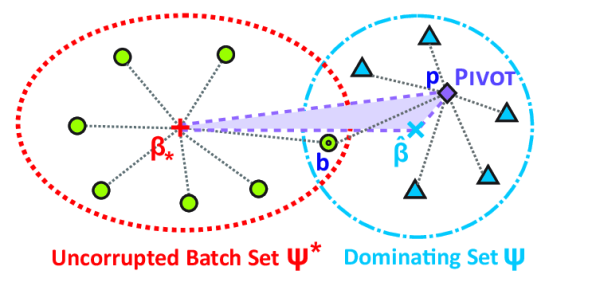
Figure 1: Example for Distributed Robust Least-squares Regression

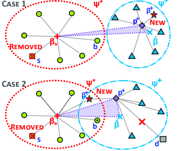
Figure 2: Examples for Online Robust Least-squares Regression

The DRLR algorithm, shown in Algorithm 2, uses $m$ mini-batches’ data as input and outputs the consolidated estimate of regression coefficients $\hat{\bm{\beta}}$. First, the algorithm optimizes the coefficient estimate $\bm{\beta}^{(i)}$ of each mini batch in Line 1-2, then it combines all the estimates of mini-batches in terms of overall robustness via distributed robust consolidation. Specifically, the algorithm determines the pivot batch based on all the estimates in Line 3 and generates the dominating set $\Psi$ in Line 4. Finally, all the batch estimates are combined via robust consolidation in Line 5. Figure 1 shows an example of distributed robust consolidation. The domination set $\Psi$ contains $\tilde{m}$ closest batches to pivot batch $p$ and the green circle node denotes the uncorrupted batch whose distance to ground truth coefficients $\bm{\beta}_{*}$ is less than a small error bound $\varepsilon$. We call the set containing all the green circle nodes as uncorrupted batch set $\Psi^{*}$. The example shows a case that only one uncorrupted batch $b$ is contained in $\Psi$, which determines the distance between $\bm{\beta}_{*}$ and pivot batch $p$. The distance between $\bm{\beta}_{*}$ and $\hat{\bm{\beta}}$ is upper bounded by the summation of distance $d_{\bm{\beta}_{*},p}$ and $d_{\hat{\bm{\beta}},p}$.

4.3 Online Robust Regression

The DRLR algorithm, proposed in Section 4.2, provides a distributed approach when a large amount of data has been collected. In this section, we present an online robust regression algorithm, named ORLR, that incrementally updates the robust estimate based on new incoming data. Specifically, suppose the regression coefficients of the previous $m$ mini-batches $\{\bm{\beta}^{(1)},\dots,\bm{\beta}^{(m)}\}$ have been estimated by DRLR, the ORLR algorithm achieves an incremental update of robust consolidation $\hat{\bm{\beta}}$ when new incoming mini-batch data $X^{+}\in\mathbbm{R}^{p\times n}$ and $\bm{y}^{+}\in\mathbbm{R}^{n\times 1}$ are given.

The details of algorithm ORLR are shown in Algorithm 3. In Line 1, the regression coefficients $\bm{\beta}^{+}$ of the new data is optimized by HRR algorithm. The index of swapped estimate $s$ is generated in Line 2 by selecting the minimum value from $[m]\setminus\Psi$, which represents the set of estimates that are not included in dominating set $\Psi$. Since new estimates are appended to the tail of $\Pi$, the usage of minimum index ensures that the oldest corrupted estimate can be swapped out. In Line 3, the selected estimate $\bm{\beta}^{(s)}$ is removed from $\Pi$ while the new estimate $\bm{\beta}^{+}$ is appended to the tail of $\Pi$. Lines 4 through 6 re-consolidate all the estimates based on newly updated $\Pi$ in the same steps as the DRLR algorithm. It is important to note that the distance vectors used in Lines 4 and 5 are also updated corresponding to the new $\Pi$. Also, the ORLR algorithm can be invoked repeatedly for the incoming mini-batches, where the outputs $\Pi$ and $\Psi$ of the previous invocation can be used as the input of the next one.

Figure 2 shows two cases for ORLR algorithm. The first case shows the condition that the new estimate $\bm{\beta}^{+}\in\Psi^{+}$ but not belongs to $\Psi^{*}$, and estimate $s$ is removed. Although the estimate $b$ is excluded from $\Psi^{+}$, the distance $d_{\bm{\beta}_{*},p^{+}}$ can still be determined by the position of $b$. The error between $\bm{\beta}_{*}$ and $\hat{\bm{\beta}}$ can be increased, but still upper bounded by $d_{\bm{\beta}_{*},p^{+}}$ and $d_{\hat{\bm{\beta}},p^{+}}$. In the second case, $\bm{\beta}^{+}\in\{\Psi^{*}\cap\Psi^{+}\}$. Because the farthest node $d$ in $\Psi^{+}$ is replaced by $\bm{\beta}^{+}$, the error between $\bm{\beta}_{*}$ and $\hat{\bm{\beta}}$ can be decreased, but it still upper bounded by the position of pivot batch $p^{+}$. Last but not least, the third case is $\bm{\beta}^{+}\notin\{\Psi^{*}\cup\Psi^{+}\}$, which is not shown in Figure 2. The case is the same as Figure 1 except a new estimate is added outside of $\Psi^{*}$ and $\Psi$. However, the change will not impact the result of $\hat{\bm{\beta}}$.

Input: New incoming corrupted data $X^{+}\in\mathbbm{R}^{p\times n}$ and $\bm{y}^{+}\in\mathbbm{R}^{n\times 1}$. Previous $m$ mini-batch estimates $\Pi=\{\bm{\beta}^{(1)},\dots,\bm{\beta}^{(m)}\}$ and their corresponding $\Psi$.

Output: solution $\hat{\bm{\beta}}$, $\Pi$, $\Psi$

1 $\bm{\beta}^{+}\leftarrow\operatorname*{\sc HRR}(X^{+},\bm{y}^{+})$

$s\leftarrow\min([m]\setminus\Psi)$

  // Select removed estimate $s$

2 $\Pi^{+}=\Pi\setminus\{\bm{\beta}^{(s)}\}\ \cup\{\bm{\beta}^{+}\}$

$p^{+}=\operatorname*{arg\,min}_{i}\sigma_{\tilde{m}}(\bm{d}^{(i)})$

  // Optimize new pivot batch $p^{+}$

$\Psi^{+}=\big{\{}\delta_{k}(\bm{d}^{(p^{+})})|1\leq k\leq\tilde{m}\big{\}}$

  // Find new dominating set $\Psi^{+}$

$\hat{\bm{\beta}}=\operatorname*{arg\,min}_{\bm{\beta}}\big{\{}\frac{1}{\tilde{m}}\sum_{i\in\Psi^{+}}\lVert\bm{\beta}^{(i)}-\bm{\beta}\rVert_{2}\big{\}}$

  // Robust consolidation

return $\hat{\bm{\beta}},\Pi^{+},\Psi^{+}$

Algorithm 3 Orlr Algorithm

5 Theoretical Recovery Analysis

In this section, the recovery properties of regression coefficients for the proposed distributed and online algorithms are presented in Theorem 4 and 5, respectively. Before that, the recovery property of HRR is presented in Theorem 1.

To prove the theoretical recovery of regression coefficients for a single mini-batch, we require that the least-squares function satisfies the Subset Strong Convexity (SSC) and Subset Strong Smoothness (SSS) properties, which are defined as follows:

Definition 6 (SSC and SSS Properties).

The least squares function $f(\bm{\beta})=\lVert\bm{y}_{S}-X_{S}^{T}\bm{\beta}\rVert_{2}^{2}$ satisfies the $2\zeta_{\gamma}$-Subset Strong Convexity property and $2\kappa_{\gamma}$-Subset Strong Smoothness property if the following holds:

$$\zeta_{\gamma}I\preceq \frac{1}{2}\triangledown^{2}f_{S}(\bm{\beta})\preceq\kappa_{\gamma}I\ \ \ \operatorname*{for}\ \forall S\in S_{\gamma}$$ (10)

Note that Equation (10) is equivalent to:

$$\zeta_{\gamma}\leq\min_{S\in S_{\gamma}}\lambda_{min}(X_{S}X_{S}^{T})\leq\max_{S\in S_{\gamma}}\lambda_{max}(X_{S}X_{S}^{T})\leq\kappa_{\gamma}$$ (11)

where $\lambda_{min}$ and $\lambda_{max}$ denote the smallest and largest eigenvalues of matrix $X$, respectively.

Theorem 1 (HRR Recovery Property).

Let $X^{(i)}\in\mathbbm{R}^{p\times n}$ be the given data matrix of the $i\textsuperscript{th}$ mini batch and the corrupted response vector $\bm{y}^{(i)}={\big{[}\bm{X}^{(i)}\big{]}}^{T}\bm{\beta}_{*}+\bm{u}^{(i)}+\bm{\varepsilon}^{(i)}$ with $\|\bm{u}^{(i)}\|_{0}=\gamma n$. Let $\Sigma_{0}$ be an invertible matrix such that $\tilde{X}^{(i)}=\Sigma_{0}^{-1/2}X^{(i)}$; $f(\bm{\beta})=\lVert\bm{y}^{(i)}_{S}-\tilde{X}^{(i)}_{S}\bm{\beta}\rVert_{2}^{2}$ satisfies the SSC and SSS properties at level $\alpha$, $\gamma$ with $2\zeta_{\alpha,\gamma}$ and $2\kappa_{\alpha,\gamma}$. If the data satisfies $\frac{\varphi_{\alpha,\gamma}}{\sqrt{\zeta_{\alpha}}}<\frac{1}{2}$, after $t=\mathcal{O}\left(\log_{\frac{1}{\eta}}\frac{\lVert\bm{u}^{(i)}\rVert_{2}}{\sqrt{n}\epsilon}\right)$ iterations, Algorithm 1 yields an $\epsilon$-accurate solution $\bm{\beta}^{(i)}_{t}$ with $\lVert\bm{\beta}_{*}-\bm{\beta}^{(i)}_{t}\rVert_{2}\leq\epsilon+\frac{C\lVert\bm{\varepsilon}^{(i)}\rVert_{2}}{\sqrt{n}}$ for some $C>0$.

The proof of Theorem 1 can be found in the supplementary material. The theoretical analyses of regression coefficients recovery for Algorithm 2 and 3 are shown in the following.

Lemma 2.

Suppose Algorithm 1 yields an $\epsilon$-accurate solution $\hat{\bm{\beta}}$ with corruption ratio $\gamma_{0}$, and $m$ mini-batches of data have a corruption ratio less than $\gamma_{0}/2$, more than $\lfloor\frac{m}{2}\rfloor+1$ batches can yield an $\epsilon$-accurate solution by Algorithm 1.

Proof.

Let $\Psi_{*}$ denote the set of mini-batches that yield $\epsilon$-accurate solutions and $\gamma_{i}$ represent the corruption ratio for the $i\textsuperscript{th}$ mini-batch. Then we have:

$$\sum_{i\in[m]\setminus\Psi_{*}}\gamma_{i}n\stackrel{{\scriptstyle(a)}}{{\leq}} \sum_{i}^{m}\gamma_{i}n=\frac{\gamma_{0}}{2}\cdot m\cdot n$$

$$(\gamma_{0}n+1)(m-\lvert\Psi_{*}\rvert)\stackrel{{\scriptstyle(b)}}{{\leq}} \frac{\gamma_{0}}{2}\cdot m\cdot n$$

Inequality (a) is based on $\sum_{i}^{m}\gamma_{i}n=\sum_{i\in\Psi_{*}}\gamma_{i}n+\sum_{i\in[m]\setminus\Psi_{*}}\gamma_{i}n$. And inequality (a) follows each corrupted mini-batch that contains at least $\gamma_{0}n+1$ corrupted samples. Applying simple algebra steps, we have

$$\lvert\Psi_{*}\rvert\geq m-\frac{\frac{\gamma_{0}}{2}mn}{\gamma_{0}n+1}\geq m-\frac{\frac{\gamma_{0}}{2}mn}{\gamma_{0}n}\geq\frac{m}{2}$$

Since $\lvert\Psi_{*}\rvert$ is an integer, then we have $\lvert\Psi_{*}\rvert\geq\lfloor\frac{m}{2}\rfloor+1$.

∎

Lemma 3.

Given a set of mini-batch estimates $\{\bm{\beta}^{(1)},\dots,\bm{\beta}^{(m)}\}$ with $\tilde{m}=\lfloor m/2\rfloor+1$, defining the $p\textsuperscript{th}$ batch as its pivot batch, then we have $\sigma_{\tilde{m}}(\bm{d}^{(p)})\leq 2\epsilon$.

Proof.

Suppose $k\textsuperscript{th}$ mini-batch is in the uncorrupted set $\Psi_{*}$, we have $\lVert\bm{\beta}^{(k)}-\bm{\beta}_{*}\rVert_{2}\leq\epsilon$. Similarly, for $\forall i\in\Psi_{*}$, we have $\lVert\bm{\beta}^{(i)}-\bm{\beta}_{*}\rVert_{2}\leq\epsilon$. According to the triangle inequality, for $\forall i\in\Psi_{*}$, it satisfies:

$$\lVert\bm{\beta}^{(i)}-\bm{\beta}^{(k)}\rVert_{2}-\lVert\bm{\beta}^{(k)}-\bm{\beta}_{*}\rVert_{2}\leq \lVert\bm{\beta}^{(i)}-\bm{\beta}_{*}\rVert_{2}\leq\epsilon$$

$$\lVert\bm{\beta}^{(i)}-\bm{\beta}^{(k)}\rVert_{2}\leq 2\epsilon$$

Since $\lvert\Psi_{*}\rvert\geq\tilde{m}$, we have $\sigma_{\tilde{m}}(\bm{d}^{(k)})\leq 2\epsilon$. According to the definition of pivot batch $p=\operatorname*{arg\,min}_{i}\sigma_{\tilde{m}}(\bm{d}^{(i)})$, we have $\sigma_{\tilde{m}}(\bm{d}^{(p)})\leq\sigma_{\tilde{m}}(\bm{d}^{(k)})\leq 2\epsilon$. ∎

Theorem 4 (DRLR Recovery Property).

Given data samples in $m$ mini batches $\{(X^{(1)},\bm{y}^{(1)}),\dots,(X^{(m)},\bm{y}^{(m)})\}$ with a corruption ratio of $\gamma_{0}/2$, Algorithm 2 yields an $\epsilon$-accurate solution $\hat{\bm{\beta}}$ with $\lVert\hat{\bm{\beta}}-\bm{\beta}_{*}\rVert_{2}\leq 5\epsilon$.

Proof.

Let $\Psi_{*}$ denotes the set of mini-batches that yield $\epsilon$-accurate solutions. According to Lemma 2, we have $\lvert\Psi_{*}\rvert\geq\lfloor\frac{m}{2}\rfloor+1$. Because of Lemma 3, we have $\forall i\in[1,\tilde{m}]$, $\sigma_{i}(\bm{d}^{(p)})\leq 2\epsilon$, where $p$ is the index of pivot batch and $\tilde{m}=\lfloor m/2\rfloor+1$. Using $\Psi=\big{\{}\delta_{k}(\bm{d}^{(p)})|1\leq k\leq\tilde{m}\big{\}}$ defined in Algorithm 2, we have $\forall i,j\in\Psi$, $\lVert\bm{\beta}^{(i)}-\bm{\beta}^{(j)}\rVert_{2}\leq 2\epsilon$. As $\lvert\Psi_{*}\rvert\geq\lfloor\frac{m}{2}\rfloor+1$, we have $\lvert\Psi_{*}\cap\Psi\rvert\geq 1$. For any $k\in\{\Psi_{*}\cap\Psi\}$, we have the following two properties of the $k\textsuperscript{th}$ mini batch: 1) $\forall i\in\Psi$, $\lVert\bm{\beta}^{(k)}-\bm{\beta}^{(i)}\rVert_{2}\leq 2\epsilon$; and 2) $\lVert\bm{\beta}^{(k)}-\bm{\beta}_{*}\rVert_{2}\leq\epsilon$. Applying these properties, we get the error bound of $\lVert\hat{\bm{\beta}}-\bm{\beta}_{*}\rVert_{2}$ as follows.

$$\lVert\hat{\bm{\beta}}-\bm{\beta}_{*}\rVert_{2}= \lVert\hat{\bm{\beta}}-\bm{\beta}^{(k)}+\bm{\beta}^{(k)}-\bm{\beta}_{*}\rVert_{2}$$

$$\stackrel{{\scriptstyle(a)}}{{\leq}} \lVert\hat{\bm{\beta}}-\bm{\beta}^{(k)}\rVert_{2}+\lVert\bm{\beta}^{(k)}-\bm{\beta}_{*}\rVert_{2}$$

$$\stackrel{{\scriptstyle(b)}}{{\leq}} \frac{1}{\tilde{m}}\sum_{i\in\Psi}\lVert\hat{\bm{\beta}}-\bm{\beta}^{(i)}\rVert_{2}+\frac{1}{\tilde{m}}\sum_{i\in\Psi}\lVert\bm{\beta}^{(i)}-\bm{\beta}^{(k)}\rVert_{2}+\epsilon$$

$$\stackrel{{\scriptstyle(c)}}{{\leq}} \frac{1}{\tilde{m}}\sum_{i\in\Psi}\lVert\bm{\beta}^{(k)}-\bm{\beta}^{(i)}\rVert_{2}+3\epsilon\leq 5\epsilon$$

Inequality (a) is based on the triangle inequality of the $L_{2}$ norm, and inequality (b) follows $\lVert\hat{\bm{\beta}}-\bm{\beta}^{(k)}\rVert_{2}=\frac{1}{T}\sum_{i\in\Psi}\lVert\hat{\bm{\beta}}-\bm{\beta}^{(i)}+\bm{\beta}^{(i)}-\bm{\beta}^{(k)}\rVert_{2}$. Inequity (c) follows the definition of $\hat{\bm{\beta}}$, which makes $\sum_{i\in\Psi}\lVert\hat{\bm{\beta}}-\bm{\beta}^{(i)}\rVert\leq\sum_{i\in\Psi}\lVert\bm{\beta}^{(k)}-\bm{\beta}^{(i)}\rVert$. ∎

Theorem 5 (ORLR Recovery Property).

Given $m$ mini-batch estimates of regression coefficients $\Pi=\{\bm{\beta}^{(1)},\dots,\bm{\beta}^{(m)}\}$, their corresponding dominating set $\Psi$, and incoming corrupted data $X^{+}\in\mathbbm{R}^{p\times n}$ and $\bm{y}^{+}\in\mathbbm{R}^{n\times 1}$, Algorithm 3 yields an $\epsilon$-accurate solution $\hat{\bm{\beta}}$ with $\lVert\hat{\bm{\beta}}-\bm{\beta}_{*}\rVert_{2}\leq 5\epsilon+\frac{4\epsilon}{\tilde{m}}$.

Proof.

Let $e$ and $s$ denote the index of added and removed mini-batch, respectively. According to Line 2 in Algorithm 3, the removed batch $s\notin\Psi$. As $\lvert\Psi\cap\Psi_{*}\rvert\geq 1$, there exists a mini-batch $k\in\{\Psi\cap\Psi_{*}\}$ that satisfies: 1) $\forall i\in\Psi$, $\lVert\bm{\beta}^{(k)}-\bm{\beta}^{(i)}\rVert_{2}\leq 2\epsilon$; and 2) $\forall j\in\{\Psi^{+}\setminus e\}$, $\lVert\bm{\beta}^{(k)}-\bm{\beta}^{(j)}\rVert_{2}\leq 2\epsilon$. So we have

$$\lVert\hat{\bm{\beta}}-\bm{\beta}^{(k)}\rVert_{2}= \frac{1}{\tilde{m}}\sum_{i\in\Psi^{+}}\lVert\hat{\bm{\beta}}-\bm{\beta}^{(i)}+\bm{\beta}^{(i)}-\bm{\beta}^{(k)}\rVert_{2}$$

$$\stackrel{{\scriptstyle(a)}}{{\leq}} \frac{1}{\tilde{m}}\sum_{i\in\Psi^{+}}\lVert\hat{\bm{\beta}}-\bm{\beta}^{(i)}\rVert_{2}+\frac{1}{\tilde{m}}\sum_{i\in\Psi^{+}}\lVert\bm{\beta}^{(i)}-\bm{\beta}^{(k)}\rVert_{2}$$

$$\stackrel{{\scriptstyle(b)}}{{\leq}} \frac{2}{\tilde{m}}\sum_{i\in\Psi^{+}}\lVert\bm{\beta}^{(i)}-\bm{\beta}^{(k)}\rVert_{2}$$

Inequality (a) is based on the triangle inequality of the $L_{2}$ norm, and inequality (b) follows the definition of $\hat{\bm{\beta}}$, which has $\sum_{i\in\Psi^{+}}\lVert\hat{\bm{\beta}}-\bm{\beta}^{(i)}\rVert\leq\sum_{i\in\Psi^{+}}\lVert\bm{\beta}^{(k)}-\bm{\beta}^{(i)}\rVert$.

Two conditions exist for added mini batch $e$. For the condition $e\notin\Psi^{+}$, the new dominating set $\Psi^{+}=\Psi$. So $\lVert\hat{\bm{\beta}}-\bm{\beta}^{(k)}\rVert_{2}\leq$ $\frac{2}{\tilde{m}}\sum_{i\in\Psi}\lVert\bm{\beta}^{(i)}-\bm{\beta}^{(k)}\rVert_{2}\leq 4\epsilon$. For condition $e\in\Psi^{+}$, we have

$$\lVert\hat{\bm{\beta}}-\bm{\beta} {}^{(k)}\rVert_{2}\leq\frac{2}{\tilde{m}}\sum_{i\in\Psi^{+}}\lVert\bm{\beta}^{(i)}-\bm{\beta}^{(k)}\rVert_{2}$$

$$\stackrel{{\scriptstyle(c)}}{{\leq}} \frac{2}{\tilde{m}}\bigg{(}\lVert\bm{\beta}^{(k)}-\bm{\beta}^{(e)}\rVert_{2}+\sum_{i\in\{\Psi^{+}\cap\Psi\}}\lVert\bm{\beta}^{(i)}-\bm{\beta}^{(k)}\rVert_{2}\bigg{)}$$

$$\stackrel{{\scriptstyle(d)}}{{\leq}} \frac{4\epsilon}{\tilde{m}}(\tilde{m}-1)+\frac{2}{\tilde{m}}\bigg{(}\lVert\bm{\beta}^{(k)}-\bm{\beta}^{(p)}\rVert_{2}+\lVert\bm{\beta}^{(p)}-\bm{\beta}^{(e)}\rVert_{2}\bigg{)}$$

$$\stackrel{{\scriptstyle(e)}}{{\leq}} \frac{4\epsilon}{\tilde{m}}(\tilde{m}-1)+\frac{8\epsilon}{\tilde{m}}\leq 4\epsilon+\frac{4\epsilon}{\tilde{m}}$$

Inequality (c) expands the set $\Psi^{+}$ into the new mini batch $e$ and set $\{\Psi^{+}\cap\Psi\}$. Inequality (d) uses the fact that $\forall i\in\Psi$, $\lVert\bm{\beta}^{(k)}-\bm{\beta}^{(i)}\rVert_{2}\leq 2\epsilon$ and the triangle inequality of $\bm{\beta}^{(p)}$, where $p$ is the pivot batch corresponding to $\Pi$. As $\max(\lVert\bm{\beta}^{(k)}-\bm{\beta}^{(p)}\rVert_{2},\lVert\bm{\beta}^{(p)}-\bm{\beta}^{(e)}\rVert_{2})\leq 2\epsilon$, inequality (e) is satisfied. Combining two conditions, we conclude $\lVert\hat{\bm{\beta}}-\bm{\beta}^{(k)}\rVert_{2}\leq 4\epsilon+\frac{4\epsilon}{\tilde{m}}$. Therefore, the error bound of $\lVert\hat{\bm{\beta}}-\bm{\beta}_{*}\rVert_{2}$ is as follows.

$$\lVert\hat{\bm{\beta}}-\bm{\beta}_{*}\rVert_{2}\leq \lVert\hat{\bm{\beta}}-\bm{\beta}^{(k)}\rVert_{2}+\lVert\bm{\beta}^{(k)}-\bm{\beta}_{*}\rVert_{2}$$

$$\stackrel{{\scriptstyle(f)}}{{\leq}} 4\epsilon+\frac{4\epsilon}{\tilde{m}}+\epsilon\leq 5\epsilon+\frac{4\epsilon}{\tilde{m}}$$

Inequality (f) utilizes the fact that $\lVert\bm{\beta}^{(k)}-\bm{\beta}_{*}\rVert_{2}\leq\epsilon$. Note that if $\tilde{m}$ is large enough, $\lVert\hat{\bm{\beta}}-\bm{\beta}_{*}\rVert_{2}\precsim 5\epsilon$, which is the same as the error bound in Theorem 4.

∎

6 Experiment

In this section, the proposed algorithms DRLR and ORLR are evaluated on both synthetic and real-world datasets. After the experiment setup has been introduced in Section 6.1, we present results on the effectiveness of the methods against several existing methods on both synthetic and real-world datasets, along with an analysis of efficiency for all the comparison methods, in Section 6.2. All the experiments were conducted on a 64-bit machine with an Intel(R) Core(TM) quad-core processor (i7CPU@3.6GHz) and 32.0GB memory. Details of both the source code and datasets used in the experiment can be downloaded here.

6.1 Experiment Setup

6.1.1 Datasets and Labels

Our dataset is composed of synthetic and real-world data. The simulation samples were randomly generated according to the model in Equation (1) for each mini-batch, sampling the regression coefficients $\bm{\beta}_{*}\in\mathbbm{R}^{p}$ as a random unit norm vector. The covariance data $X^{(i)}$ for each mini-batch was drawn independently and identically distributed from $\bm{x}_{i}\sim\mathcal{N}(0,I_{p})$ and the uncorrupted response variables were generated as $\bm{y}^{(i)}_{*}={\big{[}\bm{X}^{(i)}\big{]}}^{T}\bm{\beta}_{*}+\bm{\varepsilon}^{(i)}$, where the additive dense noise was $\varepsilon^{(i)}_{i}\sim\mathcal{N}(0,\sigma^{2})$. The corrupted response vector for each mini-batch was generated as $\bm{y}^{(i)}=\bm{y}^{(i)}_{*}+\bm{u}^{(i)}$, where the corruption vector $\bm{u}^{(i)}$ was sampled from the uniform distribution $[-5\|\bm{y}^{(i)}_{*}\|_{\infty},5\|\bm{y}^{(i)}_{*}\|_{\infty}]$. The set of uncorrupted points $Z^{(i)}_{*}$ was selected as a uniformly random $\gamma^{(i)}n$-sized subset of $[n]$, where $\gamma^{(i)}$ is the corruption ratio of the $i\textsuperscript{th}$ mini-batch. We define $\gamma$ as the corruption ratio of the total $m$ mini-batches; $\gamma^{(i)}$ is randomly chosen in the condition of $\gamma=\sum_{i}^{m}\gamma^{(i)}$, where $\gamma$ should be less than $1/2$ to ensure the number of uncorrupted samples is greater than the number of corrupted ones.

The real-world datasets we use contain house rental transaction data from New York City and Los Angeles on Airbnb website from January 2015 to October 2016. The datasets can be downloaded here. For the New York City dataset, we use the first 321,530 data samples from January 2015 to December 2015 as training data and the remaining 329,187 samples from January to October 2016 as testing data. For the Los Angeles dataset, the first 106,438 samples from May 2015 to May 2016 are chosen as training data, and the remaining 103,711 samples are used as testing data. In each dataset, there were 21 features after data preprocessing, including the number of beds and bathrooms, location, and average price in the area.

6.1.2 Evaluation Metrics

For the synthetic data, we measured the performance of the regression coefficients recovery using the averaged $L_{2}$ error

$$\small e=\lVert\hat{\bm{\beta}}-\bm{\beta}_{*}\rVert_{2}$$

where $\hat{\bm{\beta}}$ represents the recovered coefficients for each compared method and $\bm{\beta}_{*}$ is the ground truth regression coefficients. To compare the scalability of each method, the CPU running time for each of the competing methods was also measured.

For the real-world dataset, we use the mean absolute error (MAE) to evaluate the performance of rental price prediction. Defining $\hat{\bm{y}}$ and $\bm{y}$ as the predicted price and ground truth price, respectively, the mean absolute error between $\hat{\bm{y}}$ and $\bm{y}$ can be presented as follows.

$$\small\operatorname*{MAE}(\hat{\bm{y}},\bm{y})=\frac{1}{n}\sum_{i=1}^{n}\big{|}\hat{\bm{y}_{i}}-\bm{y}_{i}\big{|}$$

(a) p=100, n=5K, b=10, dense noise

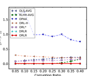
(b) p=100, n=10K, b=10, dense noise

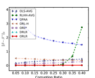
(c) p=400, n=10K, b=10, dense noise

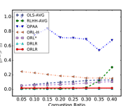
(d) p=100, n=10K, b=30, dense noise

(e) p=100, n=5K, b=10, no dense noise

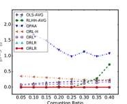
(f) p=200, n=10K, b=20, no dense noise

Figure 3: Performance on regression coefficients recovery for different corruption ratios in uniform distribution.

6.1.3 Comparison Methods

The following methods are included in the performance comparison presented here: The averaged ordinary least-squares (OLS-AVG) method takes the average over the regression coefficients of each mini-batch, which is computed by the ordinary least-squares method. RLHH-AVG applies a recently proposed robust method, RLHH [8], on each mini-batch and averages the regression coefficients of all the mini-batches. Different from OLS-AVG, RLHH-AVG can estimate the corrupted samples in each mini-batch by a heuristic method. The online passive aggressive algorithm (OPAA) [22] is an online algorithm for adaptive linear regression, which updates the model incrementally for each new data sample. We set the threshold parameter $\xi$, which controls the inaccuracy sensitively, to 22. We also compared our method to an online robust learning approach (ORL) [33], which addresses both the robustness and scalability issues in the regression problem. As the method requires a parameter for the corruption ratio, which is difficult to estimate in practice, we chose two versions with different parameter settings: ORL* and ORL-H. ORL* uses the true corruption ratio as its parameter, and ORL-H sets the outlier fraction $\lambda$ to 0.5, which is a recommended setting in [33] if it is unknown. For our proposed methods, we use DRLR and ORLR to evaluate our methods in both distributed and online settings. For ORLR, we set the number of previous mini-batch estimates to seven if not specified. All the results from comparison methods will be averaged over 10 runs.

Table 2: Performance on Regression Coefficients Recovery                              in Different Corrupted Mini-batches

	0/20	1/20	2/20	4/20	6/20	8/20
OLS-AVG	0.126	0.133	0.147	0.169	0.193	0.208
RLHH-AVG	0.011	0.065	0.096	0.131	0.163	0.185
OPAA	1.537	1.577	1.385	1.573	1.539	1.483
ORL-H	0.346	0.362	0.358	0.392	0.417	0.442
ORL*	0.078	0.089	0.092	0.106	0.113	0.150
ORLR	0.025	0.026	0.027	0.026	0.026	0.026
DRLR	0.015	0.015	0.015	0.015	0.015	0.015

Table 3: Mean Absolute Error of Rental Price Prediction

	New York City (Corruption Ratio)
	5%	10%	20%	30%	40%	Avg.
OLS-AVG	3.256$\pm$0.449	3.519$\pm$0.797	3.976$\pm$0.786	4.230$\pm$1.292	4.356$\pm$1.582	3.867$\pm$0.981
RLHH-AVG	2.823$\pm$0.000	2.824$\pm$0.000	13.092$\pm$25.354	35.184$\pm$37.426	42.713$\pm$19.304	19.327$\pm$16.417
OPAA	91.287$\pm$51.475	100.864$\pm$72.239	121.087$\pm$64.618	92.735$\pm$38.063	152.479$\pm$57.553	111.690$\pm$56.790
ORL-H	6.832$\pm$0.004	6.828$\pm$0.007	6.732$\pm$0.240	6.803$\pm$0.107	6.573$\pm$0.189	6.754$\pm$0.109
ORL*	6.538$\pm$0.293	6.384$\pm$0.274	6.394$\pm$0.208	6.406$\pm$0.180	6.471$\pm$0.190	6.439$\pm$0.229
DRLR	2.824$\pm$0.000	2.824$\pm$0.000	2.823$\pm$0.000	3.185$\pm$0.523	4.342$\pm$1.784	3.200$\pm$0.461
ORLR	2.824$\pm$0.001	2.824$\pm$0.000	2.823$\pm$0.000	2.883$\pm$0.187	3.563$\pm$0.935	2.983$\pm$0.225

	Los Angeles (Corruption Ratio)
	5%	10%	20%	30%	40%	Avg.
OLS-AVG	4.641$\pm$0.664	4.876$\pm$0.948	5.607$\pm$1.349	6.199$\pm$1.443	6.797$\pm$2.822	5.624$\pm$1.445
RLHH-AVG	3.994$\pm$0.002	3.998$\pm$0.003	4.092$\pm$0.290	28.788$\pm$47.322	30.414$\pm$35.719	14.257$\pm$16.667
OPAA	150.668$\pm$52.344	209.298$\pm$124.058	113.267$\pm$44.270	121.880$\pm$55.938	146.425$\pm$104.995	148.308$\pm$76.321
ORL-H	6.819$\pm$0.045	6.745$\pm$0.039	6.667$\pm$0.084	6.619$\pm$0.300	6.317$\pm$0.394	6.633$\pm$0.172
ORL*	6.257$\pm$0.497	6.303$\pm$0.304	6.415$\pm$0.172	6.308$\pm$0.377	6.186$\pm$0.531	6.294$\pm$0.376
DRLR	3.995$\pm$0.005	3.999$\pm$0.008	3.993$\pm$0.003	4.837$\pm$1.108	6.336$\pm$2.388	4.632$\pm$0.702
ORLR	3.997$\pm$0.008	3.999$\pm$0.009	3.994$\pm$0.004	4.466$\pm$1.141	5.802$\pm$1.990	4.452$\pm$0.630

(a) p=200, n=5K, b=10, no dense noise

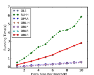
(b) p=100, cr=0.4, b=10, dense noise

(c) p=100, cr=0.4, n=5K, dense noise

Figure 4: Running time for different corruption ratios and data sizes

6.2 Performance

This section presents the recovery performance of the regression coefficients.

6.2.1 Recovery of regression coefficients

We selected seven competing methods with which to evaluate the recovery performance of all the mini-batches: OLS-AVG, RLHH-AVG, OPAA, ORL-H, ORL*, DRLR, and ORLR. Figure 3 shows the performance of coefficients recovery for different corruption ratios in uniform distribution. Specifically, Figures 3(a) and 3(b) show the recovery performance for different data sizes when the feature number is fixed. Looking at the results, we can conclude: 1) The DRLR and ORLR methods outperform all the competing methods, including ORL*, whose corruption ratio parameter uses the ground truth value. Also, the error of the ORLR method has a small difference compared to DRLR, which indicates that the online robust consolidation performs as well as the distributed one. 2) The results of the ORL methods are significantly affected by their corruption ratio parameters; ORL-H performs almost three times as badly as ORL* when the corruption ratio is less than 25%. When the corruption ratio increases, the error of ORL-H decreases because the actual corruption ratio is closer to 0.5, which is the estimated corruption ratio of ORL-H. However, both DRLR and ORLR perform consistently throughout, with no impact of the parameter. 3) RLHH-AVG has very competitive performance when the corruption ratio is less than 30% because almost no mini-batch contains corrupted samples larger than 50% when the corruption samples are randomly chosen. However, when the corruption ratio increases, some of the batches may contain large amounts of outliers, which makes some estimates be arbitrarily poor and break down the overall performance. Thus, although RLHH-AVG works well on mini-batches with fewer outliers, it cannot handle the case when the corrupted samples are arbitrarily distributed. 4) OPAA generally exhibits worse performance than the other algorithms because the incremental update for each data sample makes it very sensitive to outliers. Figures 3(c) and 3(d) show the similar performance when the number of features and batches increases. Figures 3(e) and 3(f) show that both the DRLR and ORLR methods still outperform the other methods without dense noise, with both achieving an exact recovery of ground truth regression coefficients $\bm{\beta}_{*}$.

6.2.2 Performance on different corrupted mini-batches

Table 2 shows the performance of regression coefficient recovery in different settings of corrupted mini-batches, ranging from zero to eight corrupted mini-batches out of 20 mini-batches in total. Each corrupted mini-batch used in the experiment contains 90% corrupted samples and each uncorrupted mini-batch has 10% corrupted samples. We show the result of averaged $L_{2}$ error $\lVert\hat{\bm{\beta}}-\bm{\beta}_{*}\rVert_{2}$ in 10 different synthetic datasets with randomly ordered mini-batches. From the result in Table 2, we conclude: 1) When some mini-batches are corrupted, the DRLR method outperforms all the competing methods, and ORLR achieves the best performance compared to other online methods. 2) RLHH-AVG performs the best when no mini-batch is corrupted, but its recovery error is dramatically increased when the number of corrupted mini-batches increases. However, our methods perform consistently when the number of corrupted mini-batches increases. 3) ORL* has competitive performance in different settings of corrupted mini-batches. However, its recovery error still increases two times when the number of corrupted mini-batches increases from two to eight.

6.2.3 Result of Rental Price Prediction

To evaluate the robustness of our proposed methods in a real-world dataset, we compared the performance of rental price prediction in different corruption settings, ranging from 5% to 40%. The additional corruption was sampled from the uniform distribution $[-0.5\lvert\bm{y}_{i}\rvert,0.5\lvert\bm{y}_{i}\rvert]$, where $\lvert\bm{y}_{i}\rvert$ represents the absolute price value of the $i\textsuperscript{th}$ sample data. Table 3 shows the mean absolute error of rental price prediction and its corresponding standard deviation from 10 runs in the New York City and Los Angeles datasets. From the result, we can conclude: 1) The DRLR and ORLR methods outperform all the other methods in different corruption settings except when the corruption ratio is less than 10%. 2) The RLHH-AVG method performs the best when the corruption ratio is less than or equal to 10%. However, as the corruption ratio rises, the error increases dramatically because some mini-batches are entirely corrupted. 3) The OLS-AVG method has a very competitive performance in all the corruption settings because the deviation of sampled corruption is small, which is less than 50% from the labeled data.

6.2.4 Efficiency

To evaluate the efficiency of our proposed method, we compared the performance of all the competing methods for three different data settings: different corruption ratios, data sizes per mini-batch, and batch numbers. In general, as Figure 4 shows, we can conclude: 1) The OPAA method outperforms the other methods in the three different settings because it does not consider the robustness of the data. Also, the ORL-H and ORL* methods have performed similarly to OPAA method, as they use fixed corruption ratios without taking additional steps to estimate the corruption ratio. 2) The DRLR and ORLR methods have very competitive performance even though they take additional corruption estimation and robust consolidation steps for each mini-batch. Moreover, with increases of the corruption ratio, data size per batch, and batch number, the running time of both the DRLR and ORLR methods increases linearly, which is an important characteristic for the two methods to be extended to a large scale problem. In addition, our methods outperform the RLHH method although it only estimates the corruption for each mini-batch but ignores the overall robustness, which indicates that the corruption estimation step in our method performs more efficiently than that in RLHH.

7 Conclusion

In this paper, distributed and online robust regression algorithms, DRLR and ORLR, are proposed to handle the scalable least squares regression problem in the presence of adversarial corruption. To achieve this, we proposed a heuristic hard thresholding method to estimate the corruption set for each mini-batch and designed both online and distributed robust consolidation methods to ensure the overall robustness. We demonstrate that our algorithms can yield a constant upper bound on the coefficient recovery error of state-of-the-art robust regression methods. Extensive experiments on both synthetic data and real-world rental price data demonstrated that the proposed algorithms outperform the effectiveness of other comparable methods with competitive efficiency.

References

- [1] Andrea Zanella, Nicola Bui, Angelo Castellani, Lorenzo Vangelista, and Michele Zorzi. Internet of things for smart cities. IEEE Internet of Things journal, 1(1):22–32, 2014.
- [2] Peter J Rousseeuw and Annick M Leroy. Robust regression and outlier detection, volume 589. John wiley & sons, 2005.
- [3] B Saltzberg. Performance of an efficient parallel data transmission system. IEEE Transactions on Communication Technology, 15(6):805–811, 1967.
- [4] Yudong Chen, Constantine Caramanis, and Shie Mannor. Robust sparse regression under adversarial corruption. In ICML (3), pages 774–782, 2013.
- [5] RARD Maronna, R Douglas Martin, and Victor Yohai. Robust statistics. John Wiley & Sons, Chichester. ISBN, 2006.
- [6] Brian McWilliams, Gabriel Krummenacher, Mario Lucic, and Joachim M Buhmann. Fast and robust least squares estimation in corrupted linear models. In Advances in Neural Information Processing Systems, pages 415–423, 2014.
- [7] Kush Bhatia, Prateek Jain, and Purushottam Kar. Robust regression via hard thresholding. In Advances in Neural Information Processing Systems, pages 721–729, 2015.
- [8] Xuchao Zhang, Liang Zhao, Arnold P. Boedihardjo, and Chang-Tien Lu. Robust regression via heuristic hard thresholding. In Proceedings of the Twenty-Sixth International Joint Conference on Artificial Intelligence, IJCAI’17. AAAI Press, 2017.
- [9] Markus Baldauf and JMC Santos Silva. On the use of robust regression in econometrics. Economics Letters, 114(1):124–127, 2012.
- [10] A. M. Zoubir, V. Koivunen, Y. Chakhchoukh, and M. Muma. Robust estimation in signal processing: A tutorial-style treatment of fundamental concepts. IEEE Signal Processing Magazine, 29(4):61–80, July 2012.
- [11] Imran Naseem, Roberto Togneri, and Mohammed Bennamoun. Robust regression for face recognition. Pattern Recognition, 45(1):104–118, 2012.
- [12] Yudong Chen and Constantine Caramanis. Noisy and missing data regression: Distribution-oblivious support recovery. In Sanjoy Dasgupta and David Mcallester, editors, Proceedings of the 30th International Conference on Machine Learning (ICML-13), volume 28, pages 383–391. JMLR Workshop and Conference Proceedings, 2013.
- [13] Po-Ling Loh and Martin J Wainwright. High-dimensional regression with noisy and missing data: Provable guarantees with non-convexity. In Advances in Neural Information Processing Systems, pages 2726–2734, 2011.
- [14] Mathieu Rosenbaum, Alexandre B Tsybakov, et al. Sparse recovery under matrix uncertainty. The Annals of Statistics, 38(5):2620–2651, 2010.
- [15] John Wright and Yi Ma. Dense error correction via l1-minimization. IEEE Trans. Inf. Theor., 56(7):3540–3560, July 2010.
- [16] Nam H Nguyen and Trac D Tran. Exact recoverability from dense corrupted observations via l1-minimization. IEEE transactions on information theory, 59(4):2017–2035, 2013.
- [17] Yiyuan She and Art B. Owen. Outlier detection using nonconvex penalized regression. Journal of the American Statistical Association, 106(494):626–639, 2011.
- [18] Yudong Chen, Constantine Caramanis, and Shie Mannor. Robust sparse regression under adversarial corruption. In Sanjoy Dasgupta and David Mcallester, editors, Proceedings of the 30th International Conference on Machine Learning (ICML-13), volume 28, pages 774–782. JMLR Workshop and Conference Proceedings, May 2013.
- [19] John Duchi, Elad Hazan, and Yoram Singer. Adaptive subgradient methods for online learning and stochastic optimization. Journal of Machine Learning Research, 12(Jul):2121–2159, 2011.
- [20] Julien Mairal, Francis Bach, Jean Ponce, and Guillermo Sapiro. Online learning for matrix factorization and sparse coding. Journal of Machine Learning Research, 11(Jan):19–60, 2010.
- [21] Yaakov Engel, Shie Mannor, and Ron Meir. The kernel recursive least-squares algorithm. IEEE Transactions on signal processing, 52(8):2275–2285, 2004.
- [22] Koby Crammer, Ofer Dekel, Joseph Keshet, Shai Shalev-Shwartz, and Yoram Singer. Online passive-aggressive algorithms. Journal of Machine Learning Research, 7(Mar):551–585, 2006.
- [23] G. Mateos, J. A. Bazerque, and G. B. Giannakis. Distributed sparse linear regression. IEEE Transactions on Signal Processing, 58(10):5262–5276, Oct 2010.
- [24] Stephen Boyd, Neal Parikh, Eric Chu, Borja Peleato, and Jonathan Eckstein. Distributed optimization and statistical learning via the alternating direction method of multipliers. Foundations and Trends® in Machine Learning, 3(1):1–122, 2011.
- [25] Jeffrey Dean and Sanjay Ghemawat. Mapreduce: simplified data processing on large clusters. Communications of the ACM, 51(1):107–113, 2008.
- [26] Xuan Vinh Doan, Serge Kruk, and Henry Wolkowicz. A robust algorithm for semidefinite programming. Optimization Methods and Software, 27(4-5):667–693, 2012.
- [27] Seong-Cheol Kang, Theodora S Brisimi, and Ioannis Ch Paschalidis. Distribution-dependent robust linear optimization with applications to inventory control. Annals of operations research, 231(1):229–263, 2015.
- [28] C Cromvik and M Patriksson. On the robustness of global optima and stationary solutions to stochastic mathematical programs with equilibrium constraints, part 1: Theory. Journal of optimization theory and applications, 144(3):461–478, 2010.
- [29] Jitka Dupačová and Miloš Kopa. Robustness in stochastic programs with risk constraints. Annals of Operations Research, 200(1):55–74, 2012.
- [30] Aharon Ben-Tal, Dick Den Hertog, Anja De Waegenaere, Bertrand Melenberg, and Gijs Rennen. Robust solutions of optimization problems affected by uncertain probabilities. Management Science, 59(2):341–357, 2013.
- [31] Erick Delage and Yinyu Ye. Distributionally robust optimization under moment uncertainty with application to data-driven problems. Operations Research, 58(3):595–612, 2010.
- [32] Shekhar Sharma, Swanand Khare, and Biao Huang. Robust online algorithm for adaptive linear regression parameter estimation and prediction. Journal of Chemometrics, 30(6):308–323, 2016. cem.2792.
- [33] Jiashi Feng, Huan Xu, and Shie Mannor. Outlier robust online learning. CoRR, abs/1701.00251, 2017.