Quantum statistics of a single atom Scovil–Schulz-DuBois heat engine

Abstract

We study the statistics of the lasing output from a single atom quantum heat engine, which was originally proposed by Scovil and Schulz-DuBois (SSDB). In this heat engine model, a single three-level atom is coupled with an optical cavity, and contacted with a hot and a cold heat bath together. We derive a fully quantum laser equation for this heat engine model, and obtain the photon number distribution for both below and above the lasing threshold. With the increase of the hot bath temperature, the population is inverted and lasing light comes out. However, we notice that if the hot bath temperature keeps increasing, the atomic decay rate is also enhanced, which weakens the lasing gain. As a result, another critical point appears at a very high temperature of the hot bath, after which the output light become thermal radiation again. To avoid this double-threshold behavior, we introduce a four-level heat engine model, where the atomic decay rate does not depend on the hot bath temperature. In this case, the lasing threshold is much easier to achieve, and the double-threshold behavior disappears.

I Introduction

In 1959, Scovil and Schulz-DuBois introduced a quantum heat engine model (SSDB heat engine) Scovil and Schulz-DuBois (1959); Geusic et al. (1967), where a single three-level atom is in contact with two heat baths together (Fig. 1), and the population inversion between the levels $|e_{1}\rangle$ and $|e_{2}\rangle$ can be created by a large enough temperature difference giving rise to laser output. During one working “cycle”, one hot photon $\hbar\omega_{h}$ is absorbed, one cold photon $\hbar\omega_{c}$ is emitted, and one laser photon $\hbar\Omega_{l}$ is produced. Thus, they obtain the efficiency of the heat engine as $\eta_{\text{{ssdb}}}:=\Omega_{l}/\omega_{h}$. To guarantee the laser output, a population inversion condition is required $\exp(-\frac{\omega_{h}}{T_{h}})\geq\exp(-\frac{\omega_{c}}{T_{c}})$, which is obtained from the considerations of counting the Boltzmann factors. That simply leads to an upper bound for the SSDB efficiency $\eta_{\text{{ssdb}}}\leq 1-T_{c}/T_{h}$, which is just the Carnot limit. And it turns out that the SSDB heat engine is deeply connected with many other quantum heat engine models, e.g., the quantum absorption refrigerator Geva and Kosloff (1994); Linden et al. (2010); Chen and Li (2012); Kosloff and Rezek (2017), the electromagnetically-induced-transparency (EIT) based heat engine Harris (2016); Zou et al. (2017), and it also can be used to describe the photosynthesis process and solar cell Scully et al. (2011); Su et al. (2016).

This heat engine model gives a simple and clear demonstration for the quantum thermodynamics. But we notice that some detailed properties of this lasing heat engine, e.g., the threshold behaviour and the statistics of the output light, is still not well studied. In Ref. Scully et al. (2011), a rate equation description has been developed. In order to obtain the photon statistics, we need to go beyond the rate equation description. In this paper, we study this SSDB heat engine based on a more realistic single-atom lasing setup Meschede et al. (1985); Agarwal et al. (1986); Agarwal and Dutta Gupta (1990); Walther (2000); Teuber et al. (2015), where the three-level atom is placed in an optical cavity, and coupled with the quantized field mode, as well as in contact with two heat baths with temperatures $T_{h,c}$ Boukobza and Tannor (2006a, b, 2007); Rahav et al. (2012); Perl et al. (2017); Yuge et al. (2017); Ansari (2017). We derive the lasing equation in both semi-classical and fully quantum approaches (Scully-Lamb approach Scully and Lamb (1966, 1967); Scully and Zubairy (1997)), and analytically obtain the photon number distribution in the steady state for both above and below threshold cases.

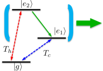
Figure 1: (Color online) Demonstration for the SSDB heat engine. A three-level atom is placed in an optical cavity to generate laser. We denote $\hbar\omega_{h}=E_{2}-E_{g}$, $\hbar\omega_{c}=E_{1}-E_{g}$, and $\hbar\Omega_{l}=E_{2}-E_{1}$.

Intuitively, a higher temperature $T_{h}$ from the hot bath enhances the population inversion between the two levels $|e_{1}\rangle$ and $|e_{2}\rangle$, and thus should also enhance lasing. However, our analytical result shows that a higher temperature $T_{h}$ also increases the atomic decay rate. As the result, the lasing gain decreases when $T_{h}$ is too high, and this system shows a “double-threshold” behavior: when the hot bath temperature $T_{h}$ is quite low ($T_{h}\simeq T_{c}$), the excitation is too weak and the system is below the lasing threshold; with the increasing of $T_{h}$, population inversion happens and the lasing light comes out; but when $T_{h}$ keeps increasing, the lasing gain starts to decrease and even goes below the threshold again, thus another critical point appears, after which the output light becomes thermal radiation again.

To avoid this double-threshold behavior, we study a four-level model where a third ancilla bath is introduced Yu and Chen (2010). In this model, neither of the two lasing levels is coupled with the hot bath directly, and thus the atomic decay rate no longer depends on the hot bath temperature. As the result, the lasing gain and cavity photon number increases monotonically and only one critical point exists. And it turns out the laser output of this four-level heat engine is also bounded by the Carnot efficiency.

We arrange the paper as follows: in Sec. II we introduce our model setup and give a semi-classical analysis; in Sec. III we study the full quantum theory, and derive the laser master equation. The master equation has the same structure as the Scully-Lamb master equations, however, with gain, loss and saturation parameters specific to the three-level model of Scovil and Schulz-DuBois. In Sec. IV, we present results for the photon statistics, we note the unusual feature that for a given gain, the photon distribution could be different. The quantum statistical features of the four-level model are presented in Sec. V. We conclude with a summary in Sec. VI. Detailed derivations are relegated to the Appendices.

II The SSDB heat engine

The heat engine model is demonstrated in Fig. 1 Boukobza and Tannor (2006b, a, 2007); Yuge et al. (2017). A three-level system, $\hat{H}_{0}=E_{g}|g\rangle\langle g|+E_{1}|e_{1}\rangle\langle e_{1}|+E_{2}|e_{2}\rangle\langle e_{2}|$, is placed in an optical cavity which is resonant with the atomic transition $|e_{1}\rangle\leftrightarrow|e_{2}\rangle$. The transition path $|e_{1/2}\rangle\leftrightarrow|g\rangle$ is coupled with a cold/hot bath.

We denote the atomic transition operators as $\hat{\tau}_{h}^{-}:=|g\rangle\langle e_{2}|,\,\hat{\tau}_{c}^{-}:=|g\rangle\langle e_{1}|$, $\hat{\sigma}^{-}:=|e_{1}\rangle\langle e_{2}|$, and $\hat{\tau}_{i}^{+}:=(\hat{\tau}_{i}^{-})^{\dagger}$, $\hat{\sigma}^{+}:=(\hat{\sigma}^{-})^{\dagger}$. The atom and the cavity interact resonantly through the Jaynes-Cummings coupling $\hat{V}=g(\hat{\sigma}^{+}\hat{a}+\hat{\sigma}^{-}\hat{a}^{\dagger})$, and the dynamics of this cavity-QED system can be described by the following master equation (interaction picture),

$$\dot{\rho}=i[\rho,\hat{V}]+{\cal L}_{h}[\rho]+{\cal L}_{c}[\rho]+{\cal L}_{\mathsf{cav}}[\rho],$$ (1)

where

$${\cal L}_{i}[\rho]= \gamma_{i}\overline{\mathsf{n}}_{i}\big{(}\hat{\tau}_{i}^{+}\rho\hat{\tau}_{i}^{-}-\frac{1}{2}\{\hat{\tau}_{i}^{-}\hat{\tau}_{i}^{+},\rho\}\big{)}$$

$$+ \gamma_{i}(\overline{\mathsf{n}}_{i}+1)\big{(}\hat{\tau}_{i}^{-}\rho\hat{\tau}_{i}^{+}-\frac{1}{2}\{\hat{\tau}_{i}^{+}\hat{\tau}_{i},\rho\}\big{)},\quad i=h,c$$

$${\cal L}_{\mathsf{cav}}[\rho]= \kappa\big{(}\hat{a}\rho\hat{a}^{\dagger}-\frac{1}{2}\hat{a}^{\dagger}\hat{a}\rho-\frac{1}{2}\rho\hat{a}^{\dagger}\hat{a}\big{)}.$$ (2)

${\cal L}_{h/c}[\rho]$ is the contribution from the hot/cold bath coupled with the atom, and ${\cal L}_{\mathsf{cav}}[\rho]$ describes the light leaking from the cavity to the outside vacuum field. Here $\overline{\mathsf{n}}_{i}:=\overline{\mathrm{n}}_{\mathrm{\textsc{p}}}(\omega_{i},T_{i})$ for $i=h,c$ is the thermal photon number of the hot/cold bath calculated from the Planck distribution $\overline{\mathrm{n}}_{\mathrm{\textsc{p}}}(\omega,T):=[\exp(\hbar\omega/k_{\text{{b}}}T)-1]^{-1}$.

With this master equation, we obtain the equations of motion

$$\frac{d}{dt}\langle\hat{\textsc{n}}_{1}\rangle =\gamma_{c}\big{[}\overline{\mathsf{n}}_{c}\langle\hat{\textsc{n}}_{g}\rangle-(\overline{\mathsf{n}}_{c}+1)\langle\hat{\textsc{n}}_{1}\rangle\big{]}-ig[\langle\hat{\sigma}^{-}\hat{a}^{\dagger}\rangle-\mathbf{h.c.}],$$

$$\frac{d}{dt}\langle\hat{\textsc{n}}_{2}\rangle =\gamma_{h}\big{[}\overline{\mathsf{n}}_{h}\langle\hat{\textsc{n}}_{g}\rangle-(\overline{\mathsf{n}}_{h}+1)\langle\hat{\textsc{n}}_{2}\rangle\big{]}+ig[\langle\hat{\sigma}^{-}\hat{a}^{\dagger}\rangle-\mathbf{h.c.}],$$

$$\frac{d}{dt}\langle\hat{\sigma}^{-}\rangle =ig\langle\hat{\sigma}^{z}\hat{a}\rangle-\frac{1}{2}\boldsymbol{\varGamma}\langle\hat{\sigma}^{-}\rangle,$$

$$\frac{d}{dt}\langle\hat{a}\rangle =-\frac{\kappa}{2}\langle\hat{a}\rangle-ig\langle\hat{\sigma}^{-}\rangle,$$ (3)

where we denote $\hat{\textsc{n}}_{g}:=|g\rangle\langle g|$, $\hat{\textsc{n}}_{1,2}:=|e_{1,2}\rangle\langle e_{1,2}|$ $\hat{\sigma}_{z}:=\hat{\textsc{n}}_{2}-\hat{\textsc{n}}_{1}$ for the atom operators, and

$$\boldsymbol{\varGamma}:=\gamma_{h}(\overline{\mathsf{n}}_{h}+1)+\gamma_{c}(\overline{\mathsf{n}}_{c}+1)$$ (4)

for the atomic coherence decay rate.

We apply the semi-classical approximation that $\langle\hat{\sigma}^{-}\hat{a}^{\dagger}\rangle\simeq\langle\hat{\sigma}^{-}\rangle\langle\hat{a}^{\dagger}\rangle$, $\langle\hat{\sigma}^{z}\hat{a}\rangle\simeq\langle\hat{\sigma}^{z}\rangle\langle\hat{a}\rangle=\langle\hat{\textsc{n}}_{2}-\hat{\textsc{n}}_{1}\rangle\langle\hat{a}\rangle$, and assume the atom rapidly decays to its steady state right before the cavity evolves significantly. Thus the quantum coherence term is given by $\langle\hat{\sigma}^{-}\rangle=(2ig/\boldsymbol{\varGamma})\langle\hat{\textsc{n}}_{2}-\hat{\textsc{n}}_{1}\rangle\langle\hat{a}\rangle$ (denoting ${\cal E}:=\langle\hat{a}\rangle$), which is proportional to the population inversion $\Delta\mathrm{N}$:

$$\Delta\mathrm{N}: =\langle\hat{\textsc{n}}_{2}-\hat{\textsc{n}}_{1}\rangle=\cfrac{\overline{\mathsf{n}}_{h}-\overline{\mathsf{n}}_{c}}{\boldsymbol{\Phi}+\frac{4g^{2}|{\cal E}|^{2}}{\boldsymbol{\varGamma}}\boldsymbol{\Psi}}$$ (5)

$$\boldsymbol{\Psi}: =\frac{1}{\gamma_{h}\gamma_{c}}[\gamma_{h}(3\overline{\mathsf{n}}_{h}+1)+\gamma_{c}(3\overline{\mathsf{n}}_{c}+1)],$$

$$\boldsymbol{\Phi}: =3\overline{\mathsf{n}}_{h}\overline{\mathsf{n}}_{c}+2(\overline{\mathsf{n}}_{h}+\overline{\mathsf{n}}_{c})+1.$$

Notice that when there is no cavity coupling ($g=0$), the atomic populations return to the SSDB result

$$\langle\hat{\textsc{n}}_{g}\rangle:\langle\hat{\textsc{n}}_{1}\rangle:\langle\hat{\textsc{n}}_{2}\rangle=1:\frac{\overline{\mathsf{n}}_{c}}{\overline{\mathsf{n}}_{c}+1}:\frac{\overline{\mathsf{n}}_{h}}{\overline{\mathsf{n}}_{h}+1},$$ (6)

and the population inversion is

$$\Delta\mathrm{N}_{0}=(\overline{\mathsf{n}}_{h}-\overline{\mathsf{n}}_{c})/\boldsymbol{\Phi}.$$ (7)

We see the constant $\boldsymbol{\Phi}$ is just the normalization factor.

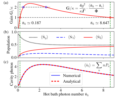
Figure 2: (Color online) (a) The lasing gain $\mathbf{G}$. $\mathbf{G}/\kappa\geq 1$ means above the lasing threshold. (b) The steady state populations on $|g\rangle$, $|e_{1,2}\rangle$. (c) The average photon number $\langle\hat{n}_{l}\rangle$ in the cavity obtained from the analytical result Eqs. (13, 17) (dashed red) and numerically solving the master equation directly (solid blue). We set $\gamma_{h}=\gamma_{c}=32\kappa$, $g=14\kappa$, and $\overline{\mathsf{n}}_{c}=0.05$ as the cold bath photon number. The two critical points are $\overline{\mathsf{n}}_{h}\simeq 0.187$ and $\overline{\mathsf{n}}_{h}\simeq 8.647$.

Now we obtain the lasing equation as

$$\dot{{\cal E}}=\big{[}\cfrac{2g^{2}(\overline{\mathsf{n}}_{h}-\overline{\mathsf{n}}_{c})}{\boldsymbol{\varGamma}\boldsymbol{\Phi}+4g^{2}|{\cal E}|^{2}\boldsymbol{\Psi}}-\frac{\kappa}{2}\big{]}{\cal E}=\frac{1}{2}\big{[}\frac{\mathbf{G}}{1+\mathbf{B}|{\cal E}|^{2}}-\kappa\big{]}{\cal E}.$$ (8)

In the above bracket, $\mathbf{G}:=4g^{2}\Delta\mathrm{N}_{0}/\boldsymbol{\varGamma}$ is the lasing gain, and $\mathbf{G}/\kappa\geq 1$ means above the lasing threshold. And $\mathbf{B}:=4g^{2}\boldsymbol{\Psi}/\boldsymbol{\varGamma}\boldsymbol{\Phi}$ is the saturation parameter. It is worth noticing that, although the population inversion $\Delta\mathrm{N}_{0}$ increases with $\overline{\mathsf{n}}_{h}$, it also gets saturated and could never exceed 1, while the atomic decay rate $\boldsymbol{\varGamma}$ keeps increasing linearly with $\overline{\mathsf{n}}_{h}$.

As the result, with the increasing of $T_{h}$ starting from $T_{c}$, the lasing gain first increases from zero, and gets above the threshold; but then the lasing gain achieves a maximum point, after which it starts to decrease, and even goes below the threshold again at a very high temperature of $T_{h}$ [Fig. 2(a, b)].

Intuitively, a higher $T_{h}$ would enhance the population inversion for lasing. But a higher $T_{h}$ also enhances the atomic decay rate $\boldsymbol{\varGamma}$, and that suppresses the lasing gain [Eq. (8)]. Therefore, at a very high temperature $T_{h}$, the lasing gain decreases and even below the threshold again.

In Fig. 2(b) we show a numerical result for the atomic populations in the steady state changing with $T_{h}$. When $T_{h}$ is very high, the populations on $|e_{1,2}\rangle$ have been almost totally inverted, but the lasing gain $\mathbf{G}$ decreases with $T_{h}$. As well, the cavity photon number $\langle\hat{n}_{l}\rangle$ shows the similar behavior [Fig. 2(c)]. Notice that the photon number $\langle\hat{n}_{l}\rangle$ in the cavity is not large, this is because we have only one atom in the cavity, thus the photon emission is limited.

If the cavity coupling strength $g$ is strong, or atomic spontaneous decay rates $\gamma_{h,c}$ are weak, the second critical point would appear at a much higher temperature $T_{h}$, but such a behavior of double critical points always exists. For realistic laser systems with $N$ atoms in the cavity, the coupling strength could be effectively enhanced by the atom number ($\sqrt{N}g$). Therefore, it is not easy to observe such double-threshold behavior in common laser systems, since the second threshold is usually too high and beyond the practical regime of interests. However, for single atom heat engine laser, this double-threshold behavior is much easier to happen.

In the fine cavity limit, $\kappa\rightarrow 0$, this threshold condition simply reduces as $\overline{\mathsf{n}}_{h}-\overline{\mathsf{n}}_{c}\geq 0$, and then it leads to the SSDB inequality $\eta_{\text{{ssdb}}}=\Omega_{l}/\omega_{h}\leq 1-T_{c}/T_{h}$, which was derived based on the comparison of the Boltzmann factors Scovil and Schulz-DuBois (1959).

III Fully quantum approach

The semi-classical approach is helpful to get a basic understanding of the physics process in this heat engine. To get a more precise and rigorous description, we adopt the Scully-Lamb approach to study the fully quantum theory for the cavity mode $\varrho:=\mathrm{tr}_{\mathrm{atom}}\rho$ Scully and Lamb (1966, 1967); Scully and Zubairy (1997); Sargent et al. (1978). In this approach, the previous semi-classical separation of the correlation functions are not needed. Denoting the matrix elements of $\varrho$ in Fock basis as $P_{mn}:=\langle m|\varrho|n\rangle$, we have

$$\frac{d}{dt}P_{mn}= ig\big{(}\sqrt{n}\rho_{12;m,n-1}-\sqrt{m}\rho_{21;m-1,n}\big{)}$$

$$- ig\big{(}\sqrt{m+1}\rho_{12;m+1,n}-\sqrt{n+1}\rho_{21;m,n+1}\big{)}$$ (9)

$$+ \kappa\big{[}\sqrt{(m+1)(n+1)}P_{m+1,n+1}-\frac{1}{2}(m+n)P_{mn}\big{]}.$$

Here $\rho_{\alpha\beta;mn}:=\langle\alpha,m|\rho|\beta,n\rangle$, and $\alpha,\beta=1,2,g$ is the atom state indices. The first two terms means the dynamics of the cavity mode and the atom are coupled together, and we need to eliminate the atom degree of freedom.

Figure 3: (Color online) The photon number distributions and Wigner functions. The parameters are the same with those in Fig. 2, and (a, b) $\overline{\mathsf{n}}_{h}=0.17$ (below threshold) (c, d) $\overline{\mathsf{n}}_{h}=0.507$ (above threshold) (e, f) $\overline{\mathsf{n}}_{h}=2.629$ (above threshold) (g, h) $\overline{\mathsf{n}}_{h}=9$ (below threshold). Notice that $\overline{\mathsf{n}}_{h}=0.507$ (c, d) and $\overline{\mathsf{n}}_{h}=2.629$ (e, f) are the two blue points in Fig. 2(a) which have the same gain $\mathbf{G}/\kappa=2$. The two critical points are $\overline{\mathsf{n}}_{h}\simeq 0.187$ and $\overline{\mathsf{n}}_{h}\simeq 8.647$. The yellow columns (right) are given by the analytical result Eq. (13), and the green columns (left) are the numerical result by solving the master equation (1) directly. The distributions below the lasing threshold (a, b, g, h) are not exactly thermal distributions ($P_{n}\propto\exp[-n\Omega_{l}/T]$). The red dashed lines in (c, e) are the corresponding Poisson distribution $P_{n}=e^{-\langle\hat{n}_{l}\rangle}\langle\hat{n}_{l}\rangle^{n}/n!$ where $\langle\hat{n}_{l}\rangle$ is the average photon number.

For this purpose, we adopt the adiabatic elimination to take away the dynamics of the atom Scully and Lamb (1966, 1967); Scully and Zubairy (1997). Namely, we assume that the atom decays very fast and quickly arrives at its steady state ($\kappa\ll\gamma_{h,c}$). That gives a set of algebraic equations, which enable us to obtain the following equation for the photon number probability $P_{n}:=\langle n|\varrho|n\rangle$ (see Appendix A),

$$\frac{d}{dt}P_{n}= \frac{n\left[\mathscr{A}P_{n-1}-\mathscr{A}_{\mathrm{b}}P_{n}\right]}{1+n\mathscr{B}/\mathscr{A}}-\frac{(n+1)\left[\mathscr{A}P_{n}-\mathscr{A}_{\mathrm{b}}P_{n+1}\right]}{1+(n+1)\mathscr{B}/\mathscr{A}}$$

$$+\kappa\left[(n+1)P_{n+1}-nP_{n}\right],$$ (10)

where we denote

$$\mathscr{A}:=\frac{4g^{2}\overline{\mathsf{n}}_{h}(\overline{\mathsf{n}}_{c}+1)}{\boldsymbol{\varGamma}\boldsymbol{\Phi}},\quad\mathscr{A}_{\mathrm{b}}=\frac{4g^{2}\overline{\mathsf{n}}_{c}(\overline{\mathsf{n}}_{h}+1)}{\boldsymbol{\varGamma}\boldsymbol{\Phi}},$$

$$\mathscr{B}:=\mathscr{A}\cdot\frac{4g^{2}\boldsymbol{\Psi}}{\boldsymbol{\varGamma}\boldsymbol{\Phi}}.$$ (11)

The constants $\boldsymbol{\varGamma}$, $\boldsymbol{\Phi}$, $\boldsymbol{\Psi}$ are the same as in Eqs. (4, 5). This equation has the same form as Ref. Sargent et al. (1978) [eq. (59) in pp. 297]. Here $\mathscr{A}$ indicates the stimulated emission rate, while $\mathscr{A}_{\mathrm{b}}$ is the stimulated absorption rate.

Expending the fractions in the above lasing equation to the 1st order, we further derive the equation for the average photon number $\langle\hat{n}_{l}\rangle=\sum nP_{n}$, i.e.,

$$\frac{d}{dt}\langle\hat{n}_{l}\rangle= \big{(}\mathscr{A}-\mathscr{A}_{\mathrm{b}}-\kappa\big{)}\langle\hat{n}_{l}\rangle$$

$$+\mathscr{A}-\mathscr{B}\langle(\hat{n}_{l}+1)^{2}\rangle+\frac{\mathscr{A}}{\mathscr{A}_{\mathrm{b}}}\cdot\mathscr{B}\langle\hat{n}_{l}^{2}\rangle\dots$$ (12)

The first linear term is the net lasing gain, which is exactly the same with that in the previous semi-classical laser equation (8), and we can verify $\mathscr{A}-\mathscr{A}_{\mathrm{b}}=\mathbf{G}$. The $\mathscr{B}$ terms are nonlinear saturation which is beyond the linearized laser theory.

IV Photon number statistics

Setting $\dot{P}_{n}=0$ in the lasing equation (10), the photon number distribution of the cavity mode in the steady state is obtained as follows:

$$\frac{P_{n}}{P_{n-1}} =\frac{\mathscr{A}}{\mathscr{A}_{\mathrm{b}}+\kappa(1+\frac{n\mathscr{B}}{\mathscr{A}})},$$ (13)

$$P_{n} =P_{0}\prod_{k=1}^{n}\frac{\mathscr{A}}{\mathscr{A}_{\mathrm{b}}+\kappa(1+\frac{k\mathscr{B}}{\mathscr{A}})}.\quad(n\geq 1)$$

The maximum probability of $P_{n}$ appears around

$$n_{*}=\frac{\mathscr{A}}{\kappa\mathscr{B}}(\mathscr{A}-\mathscr{A}_{\mathrm{b}}-\kappa).$$ (14)

$P_{n}$ increases when $n<n_{*}$ while decreases when $n>n_{*}$. Thus the lasing threshold requires $n_{*}\geq 0$, which is just the same as the above threshold condition $\mathbf{G}-\kappa=\mathscr{A}-\mathscr{A}_{\mathrm{b}}-\kappa\geq 0$.

When the system is working far below the threshold, approximately the distribution becomes an exponentially decaying one,

$$\frac{P_{n}}{P_{n-1}}=\frac{\mathscr{A}}{\mathscr{A}_{\mathrm{b}}+\kappa}\leq 1.$$ (15)

Therefore, the output light is like thermal radiation.

But we should remember if the system is below but still close to the lasing threshold, the the realistic photon distribution is not the idealistic thermal one [Eq. (13)]. For example, Fig. 3(b, c) shows that $P_{n}$ is not exactly an exponentially decaying distribution. As well, above the threshold, the distribution is not the perfect Poisson one either Scully and Lamb (1967); Scully and Zubairy (1997).

In Fig. 3, we show the photon number distributions and the corresponding Wigner functions when $T_{h}$ is in different regimes. The photon number distribution is calculated by the above analytical result Eq. (13) (yellow columns on the right), as well as by solving the master equation (1) numerically (green columns on the left), and they match each other quite well for all different $T_{h}$, which confirms the validity of the above adiabatic elimination method.

And it shows that with the increasing of $T_{h}$, the cavity output light first gives out thermal light, then becomes lasing, and turns back to be thermal again at the very high temperature regime, which confirms our previous result.

It is worth noticing that the two blue points in Fig. 2(a) ($\overline{\mathsf{n}}_{h}\simeq 0.507$ and $\overline{\mathsf{n}}_{h}\simeq 2.629$) have the same gain $\mathbf{G}$, but their distributions still differ a lot [see Fig. 3(c, e)]. For example, their maximum value also depends on $\mathscr{A}/\mathscr{B}$ [see Eq. (14)].

The total output power of the cavity is

$${\cal P}_{l}=-\mathrm{tr}\big{[}\mathcal{L}_{\mathsf{cav}}[\rho]\cdot\hbar\Omega_{l}\hat{n}_{l}\big{]}=\hbar\Omega_{l}\cdot\kappa\langle\hat{n}_{l}\rangle,$$ (16)

which is proportional to the average photon number of the cavity mode. From the photon number distribution Eq. (13), we obtain the average photon number (see Appendix A)

$$\langle\hat{n}_{l}\rangle=\frac{\mathscr{A}}{\kappa\mathscr{B}}(\mathscr{A}-\mathscr{A}_{\mathrm{b}}-\kappa)+\frac{\mathscr{A}}{\kappa\mathscr{B}}(\kappa+\mathscr{A}_{\mathrm{b}})P_{0}.$$ (17)

In Fig. 2(c), we compare this analytical result for cavity photon number with the numerical result by solving the master equation (1) directly, and they fit each other quite well.

When the system is far above the threshold, $P_{0}\simeq 0$, thus only the first term dominates. Therefore, the laser power is

$${\cal P}_{l} =\hbar\Omega_{l}\cdot\frac{\mathscr{A}}{\mathscr{B}}(\mathscr{A}-\mathscr{A}_{\mathrm{b}}-\kappa)$$

$$=\frac{\hbar\Omega_{l}\cdot\gamma_{h}\gamma_{c}(\overline{\mathsf{n}}_{h}-\overline{\mathsf{n}}_{c}-\frac{\kappa}{4g^{2}}\boldsymbol{\varGamma}\boldsymbol{\Phi})}{\gamma_{h}(3\overline{\mathsf{n}}_{h}+1)+\gamma_{c}(3\overline{\mathsf{n}}_{c}+1)}.$$ (18)

The leading term of this result (without the $\kappa$ term) is the same with that in Ref. Scully et al. (2011), which was calculated by rate equations (see eq. [S6] in supporting information). This result is valid when the system is far above the lasing threshold. When the system is below or around the threshold, the $P_{0}$ term in Eq. (17) becomes important and cannot be neglected [Fig. 2(c)]. Considering $\overline{\mathsf{n}}_{c}\sim 0$, $\gamma_{h}=\gamma_{c}=\gamma$, a rough estimation for the cavity photon number is

$$\langle\hat{n}_{l}\rangle\sim\frac{\gamma\overline{\mathsf{n}}_{h}}{\kappa(3\overline{\mathsf{n}}_{h}+2)}-\frac{\gamma^{2}}{4g^{2}}\cdot\frac{(\overline{\mathsf{n}}_{h}+1)(2\overline{\mathsf{n}}_{h}+1)}{3\overline{\mathsf{n}}_{h}+2},$$ (19)

where the second term increases with $\overline{\mathsf{n}}_{h}$ monotonically, and indicates the hot photon number could weaken the lasing. Thus the maximum cavity photon number does not appear at $\overline{\mathsf{n}}_{h}\rightarrow\infty$. Again we see that the cavity photon number is not large, and this is because there is only one single atom in the cavity, thus the photon emission is limited.

Further, with this distribution $P_{n}$, the variance of the photon number is

$$\sigma^{2}:=\langle\hat{n}_{l}^{2}\rangle-\langle\hat{n}_{l}\rangle^{2}=\frac{\mathscr{A}^{2}}{\kappa\mathscr{B}}-\frac{\mathscr{A}}{\kappa\mathscr{B}}(\kappa+\mathscr{A}_{\mathrm{b}})P_{0}\langle\hat{n}_{l}\rangle.$$ (20)

When the system is far above the threshold, $P_{0}\simeq 0$, and

$$\frac{\sigma^{2}}{\langle\hat{n}_{l}\rangle}=1+\frac{\mathscr{A}_{\mathrm{b}}+\kappa}{\mathscr{A}-\mathscr{A}_{\mathrm{b}}-\kappa}.$$ (21)

Thus the lasing photon number distribution is super-Poissonian ($\sigma^{2}>\langle\hat{n}_{l}\rangle$). When $\mathscr{A}\gg\mathscr{A}_{\mathrm{b}}+\kappa$, the photon distribution approaches the Poissonian one with $\sigma^{2}\simeq\langle\hat{n}_{l}\rangle$.

V Four-level heat engine model

In the above discussion, we notice that the three-level heat engine has a problem of double critical points, namely, when the hot bath temperature is increased, the atomic coherence decay rate is also increased, which decreases the lasing gain and even below the threshold again. To avoid this problem, we consider a four-level system as shown in Fig. 4 Yu and Chen (2010). The transition $|e_{2}\rangle\leftrightarrow|e_{3}\rangle$ is coupled with a third ancilla bath with a low temperature $T_{\mathsf{a}}$, so as to “cool down” the atomic coherence decay rate of the lasing transition. Besides, this third bath also increases the population on $|e_{2}\rangle$, as we will show below.

Using the same method as the above discussion (see also Appendix B), the linearized semi-classical lasing equation is

$$\dot{{\cal E}}\simeq\frac{1}{2}\big{[}\cfrac{4g^{2}}{\boldsymbol{\varGamma}^{\prime}}\cdot\Delta\mathrm{N}_{0}^{\prime}-\kappa\big{]}{\cal E}+o(|{\cal E}|^{2}),$$

$$\Delta\mathrm{N}_{0}^{\prime}=[(\overline{\mathsf{n}}_{h}-\overline{\mathsf{n}}_{c})\overline{\mathsf{n}}_{\mathsf{a}}+(\overline{\mathsf{n}}_{c}+1)\overline{\mathsf{n}}_{h}]/\boldsymbol{\Phi}^{\prime},$$ (22)

where $\mathbf{G}^{\prime}:=4g^{2}\Delta\mathrm{N}_{0}^{\prime}/\boldsymbol{\varGamma}^{\prime}$ is the lasing gain, and

$$\boldsymbol{\varGamma}^{\prime}= \gamma_{\mathsf{a}}\overline{\mathsf{n}}_{\mathsf{a}}+\gamma_{c}(\overline{\mathsf{n}}_{c}+1),$$

$$\boldsymbol{\Phi}^{\prime}= (4\overline{\mathsf{n}}_{h}\overline{\mathsf{n}}_{c}+3\overline{\mathsf{n}}_{h}+2\overline{\mathsf{n}}_{c}+1)\overline{\mathsf{n}}_{\mathsf{a}}+\overline{\mathsf{n}}_{h}(\overline{\mathsf{n}}_{c}+1).$$ (23)

Here $\overline{\mathsf{n}}_{\mathsf{a}}:=\overline{\mathrm{n}}_{\mathrm{\textsc{p}}}(\omega_{\mathsf{a}},T_{\mathsf{a}})$ is the thermal photon number of the transition $|e_{2}\rangle\leftrightarrow|e_{3}\rangle$, and $\omega_{\mathsf{a}}=E_{3}-E_{2}$.

Figure 4: (Color online) A four-level heat engine. The transition $|e_{2}\rangle\leftrightarrow|e_{3}\rangle$ is coupled with a third ancilla bath with temperature $T_{\mathsf{a}}$.

In this case, the decay rate $\boldsymbol{\varGamma}^{\prime}$ does not depend on the hot bath, thus will not increase with $T_{h}$ as the three-level case. And it is clear to see that $\mathbf{G}^{\prime}/\kappa=1$ is a linear equation and gives only one root for $\overline{\mathsf{n}}_{h}$ when $\overline{\mathsf{n}}_{c,\mathsf{a}}$ are fixed, which means only one critical point exists (see Fig. 5).

Simple algebra shows that $\Delta\mathrm{N}_{0}^{\prime}$ is the population inversion on $|e_{2}\rangle$ and $|e_{1}\rangle$ when there is no cavity coupling. Notice that when $T_{\mathsf{a}}\rightarrow 0$, we have $\Delta\mathrm{N}_{0}^{\prime}\rightarrow 1$, which means all the populations would fall on $|e_{2}\rangle$ in the steady state. This is because when $T_{\mathsf{a}}=0$, once the population falls down from $|e_{3}\rangle$ to $|e_{2}\rangle$, it could never go back. This is the maximum inversion for lasing. In Fig. 5, we also notice that the lasing threshold is much easier to achieve comparing with the 3-level case, i.e., a very small $\overline{\mathsf{n}}_{h}$ provides a strong enough pumping for lasing.

In the finite cavity limit, $\kappa\rightarrow 0$, the lasing condition is given by $\Delta\mathrm{N}_{0}^{\prime}\geq 0$ [Eq. (22)], which leads to

$$e^{\frac{\omega_{\mathsf{a}}}{T_{\mathsf{a}}}}\cdot e^{\frac{\omega_{c}}{T_{c}}}\geq e^{\frac{\omega_{h}}{T_{h}}}.$$ (24)

If we consider the ancilla bath has the same temperature with the cold one, $T_{\mathsf{a}}=T_{c}$, the above inequality gives

$$1-\frac{T_{c}}{T_{h}}\geq 1-\frac{\omega_{\mathsf{a}}+\omega_{c}}{\omega_{h}}=\frac{\Omega_{l}}{\omega_{h}}.$$ (25)

Here $\Omega_{l}/\omega_{h}$ is just the output efficiency of this four-level system, and again it is bounded by the Carnot efficiency, which is similar as the previous SSDB discussion.

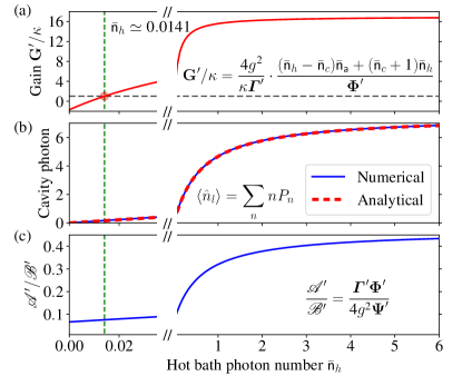
Figure 5: (Color online) (a) The lasing gain $\mathbf{G}^{\prime}$ for the four-level system. (b) The average photon number $\langle\hat{n}_{l}\rangle$ in the cavity obtained from the analytical result (dashed red) and numerically solving the master equation directly (solid blue). (c) The ratio $\mathscr{A}^{\prime}/\mathscr{B}^{\prime}$. We set $\gamma_{h}=\gamma_{c}=\gamma_{\mathsf{a}}=32\kappa$, $g=14\kappa$, and $\overline{\mathsf{n}}_{c}=0.1$, $\overline{\mathsf{n}}_{\mathsf{a}}=0.1$. The critical point is $\overline{\mathsf{n}}_{h}\simeq 0.0141$.

The full-quantum equation also has the same form as the three-level case [Eq. (10)], except the parameters $\mathscr{A}$, $\mathscr{A}_{\mathrm{b}}$, $\mathscr{B}$ should be changed to be (see Appendix B)

$$\mathscr{A}^{\prime}:=\frac{4g^{2}\overline{\mathsf{n}}_{h}(\overline{\mathsf{n}}_{c}+1)(\overline{\mathsf{n}}_{\mathsf{a}}+1)}{\boldsymbol{\varGamma}^{\prime}\boldsymbol{\Phi}^{\prime}},\quad\mathscr{A}_{\mathrm{b}}^{\prime}=\frac{4g^{2}\overline{\mathsf{n}}_{c}\overline{\mathsf{n}}_{\mathsf{a}}(\overline{\mathsf{n}}_{h}+1)}{\boldsymbol{\varGamma}^{\prime}\boldsymbol{\Phi}^{\prime}},$$

$$\mathscr{B}^{\prime}:=\mathscr{A}^{\prime}\cdot\frac{4g^{2}\boldsymbol{\Psi}^{\prime}}{\boldsymbol{\varGamma}^{\prime}\boldsymbol{\Phi}^{\prime}},$$ (26)

where $\boldsymbol{\Psi}^{\prime}=\gamma_{h}^{-1}(4\overline{\mathsf{n}}_{\mathsf{a}}\overline{\mathsf{n}}_{c}+\overline{\mathsf{n}}_{\mathsf{a}}+3\overline{\mathsf{n}}_{c}+1)+\gamma_{c}^{-1}(4\overline{\mathsf{n}}_{h}\overline{\mathsf{n}}_{\mathsf{a}}+2\overline{\mathsf{n}}_{h}+\overline{\mathsf{n}}_{\mathsf{a}})+\gamma_{\mathsf{a}}^{-1}(4\overline{\mathsf{n}}_{h}\overline{\mathsf{n}}_{c}+2\overline{\mathsf{n}}_{h}+3\overline{\mathsf{n}}_{c}+1)$. In Fig. 5 we show the lasing gain and the cavity photon number, and they all increases monotonically with the hot bath temperature $T_{h}$. Again, the laser gain is just given by $\mathbf{G}^{\prime}=\mathscr{A}^{\prime}-\mathscr{A}_{\mathrm{b}}^{\prime}$.

The cavity photon number is still given by Eq. (17), but the parameters should be changed by $\mathscr{A}^{\prime},\,\mathscr{A}_{\mathrm{b}}^{\prime}$ and $\mathbf{\mathscr{B}^{\prime}}$ correspondingly. Fig. 5(c) shows that this analytical result for the cavity photon number fits quite well with the numerical result.

When the system is far above threshold, the laser power is estimated by (considering $\kappa\rightarrow 0$)

$$\kappa\langle\hat{n}_{l}\rangle\simeq\frac{\mathbf{G}^{\prime}\mathscr{A}^{\prime}}{\mathscr{B}^{\prime}}=[(\overline{\mathsf{n}}_{h}-\overline{\mathsf{n}}_{c})\overline{\mathsf{n}}_{\mathsf{a}}+(\overline{\mathsf{n}}_{c}+1)\overline{\mathsf{n}}_{h}]/\boldsymbol{\Psi}^{\prime}.$$ (27)

If we further consider $\overline{\mathsf{n}}_{c,\mathsf{a}}\sim 0$, $\gamma_{h}=\gamma_{c}=\gamma_{\mathsf{a}}=\gamma$, $\overline{\mathsf{n}}_{h}\gg 1$, then the maximum gain and cavity photon number are around $\mathbf{G}^{\prime}\sim 4g^{2}/\gamma$ and $\langle\hat{n}_{l}\rangle\sim\gamma/4\kappa$. Both the lasing gain $\mathbf{G}^{\prime}$ and the cavity photon number $\langle\hat{n}_{l}\rangle$ approach saturated at the very high temperature regime, as shown in Fig. 5. This is because in this regime, the population has been almost totally inverted ($\Delta\mathrm{N}_{0}^{\prime}\rightarrow 1$), thus the increase of the hot bath temperature $T_{h}$ can no longer bring in a significant increase to the lasing gain. Unlike the 3-level result Eq. (19), the hot bath no longer has any weakening effect to the lasing, thus more lasing photons can be produced in the cavity, and the lasing power can be increased. But still the cavity photon number is limited due to the single atom feature.

VI Summary

In this paper, we study the statistics of the lasing output from the SSDB heat engine. In this heat engine model, a single three-level atom is coupled with the quantized cavity mode, as well as contacting with a hot and a cold heat bath together. We derive a laser equation for this heat engine model, and obtain the photon number distribution for both below and above the lasing threshold. Below the lasing threshold, the output light from the cavity is more likely thermal radiation. With the increase of the hot bath temperature, the population is inverted and lasing light comes out. If the hot bath temperature keeps increasing, our analytical result show that the atomic decay rate is also enhanced, which weakens the lasing gain. As the result, at a very high temperature of the hot bath, another critical point appears, and after that the output light become thermal radiation again.

To avoid this double-threshold behavior, we considered a four-level model where neither of the two lasing level is coupled with the hot bath directly, and a third ancilla bath is introduced. As the result, the atomic decay rate in this four-level no longer depends on the hot bath temperature, and thus the lasing gain and cavity photon number keeps increasing monotonically when the hot bath temperature increases. This four-level heat engine is also bounded by the Carnot efficiency, which is the same as the original three-level SSDB model.

Acknowledgement - This study is supported by Office of Naval Research (Award No. N00014-16-1-3054) and Robert A. Welch Foundation (Grant No. A-1261).

Appendix A Lasing equation for the three-level system

1. Lasing equation:

Here we derive the lasing equation for the photon number distribution $P_{n}=\langle n|\varrho|n\rangle$ where $\varrho=\mathrm{tr}_{\mathrm{atom}}\rho$ is the density matrix of the cavity mode. We assume the cavity leaking is much slower than the atom decay and omit ${\cal L}_{\mathsf{cav}}[\rho]$, then the master equation (1) gives (denoting $\rho_{\alpha\beta;mn}=\langle\alpha,m|\rho|\beta,n\rangle$ where $\alpha,\beta=1,2,g$ is the atom state indices)

$$\frac{d}{dt}\rho_{11;mn} =ig\left(\sqrt{n}\rho_{12;m,n-1}-\sqrt{m}\rho_{21;m-1,n}\right)-\Gamma_{c}^{-}\rho_{11;mn}+\Gamma_{c}^{+}\rho_{gg;mn},$$

$$\frac{d}{dt}\rho_{22;mn} =ig\left(\sqrt{n+1}\rho_{21;m,n+1}-\sqrt{m+1}\rho_{12;m+1,n}\right)-\Gamma_{h}^{-}\rho_{22;mn}+\Gamma_{h}^{+}\rho_{gg;mn},$$

$$\frac{d}{dt}\rho_{12;mn} =ig\left(\sqrt{n+1}\rho_{11;m,n+1}-\sqrt{m}\rho_{22;m-1,n}\right)-\frac{1}{2}(\Gamma_{h}^{-}+\Gamma_{c}^{-})\rho_{12;mn},$$ (28)

$$\frac{d}{dt}\rho_{21;mn} =-ig\left(\sqrt{m+1}\rho_{11;m+1,n}-\sqrt{n}\rho_{22;m,n-1}\right)-\frac{1}{2}(\Gamma_{h}^{-}+\Gamma_{c}^{-})\rho_{21;mn},$$

$$\frac{d}{dt}\rho_{gg;mn} =\Gamma_{c}^{-}\rho_{11;mn}-\Gamma_{c}^{+}\rho_{gg;mn}+\Gamma_{h}^{-}\rho_{22;mn}-\Gamma_{h}^{+}\rho_{gg;mn}.$$

Here we denote $\Gamma_{i}^{+}=\gamma_{i}\overline{\mathsf{n}}_{i}$ and $\Gamma_{i}^{-}=\gamma_{i}(\overline{\mathsf{n}}_{i}+1)$ for $i=h,c$. The matrix elements for the cavity mode is $P_{mn}:=\langle m|\varrho|n\rangle=\rho_{11;mn}+\rho_{22;mn}+\rho_{gg;mn}$, thus, combining with the cavity leaking term ${\cal L}_{\mathsf{cav}}[\rho]$, the equation for the cavity mode is

$$\frac{d}{dt}P_{mn}= ig\big{(}\sqrt{n}\rho_{12;m,n-1}-\sqrt{m}\rho_{21;m-1,n}\big{)}-ig\big{(}\sqrt{m+1}\rho_{12;m+1,n}-\sqrt{n+1}\rho_{21;m,n+1}\big{)}$$

$$+\kappa\big{[}\sqrt{(m+1)(n+1)}P_{m+1,n+1}-\frac{1}{2}(m+n)P_{mn}\big{]}.$$ (29)

In the first two terms, the dynamics of the cavity mode is still coupled with that of the atom.

To derive a equation for the cavity mode alone, we need to replace $\rho_{12;mn}$ by $P_{mn}$ in the above equation by adiabatic elimination Scully and Lamb (1967); Scully and Zubairy (1997). That is, due to the fast decay of the atom, Eq. (28) quickly arrives at the steady state, and that gives:

$$0 =ig\left(\sqrt{n}\rho_{12;m,n-1}-\sqrt{m}\rho_{21;m-1,n}\right)-\Gamma_{c}^{-}\rho_{11;mn}+\Gamma_{c}^{+}\rho_{gg;mn},$$

$$0 =ig\left(\sqrt{n}\rho_{21;m-1,n}-\sqrt{m}\rho_{12;m,n-1}\right)-\Gamma_{h}^{-}\rho_{22;m-1,n-1}+\Gamma_{h}^{+}\rho_{gg;m-1,n-1},$$

$$0 =ig\left(\sqrt{n}\rho_{11;mn}-\sqrt{m}\rho_{22;m-1,n-1}\right)-\frac{1}{2}(\Gamma_{h}^{-}+\Gamma_{c}^{-})\rho_{12;m,n-1},$$

$$0 =-ig\left(\sqrt{m}\rho_{11;mn}-\sqrt{n}\rho_{22;m-1,n-1}\right)-\frac{1}{2}(\Gamma_{h}^{-}+\Gamma_{c}^{-})\rho_{21;m-1,n},$$ (30)

$$0 =\Gamma_{c}^{-}\rho_{11;mn}-\Gamma_{c}^{+}\rho_{gg;mn}+\Gamma_{h}^{-}\rho_{22;mn}-\Gamma_{h}^{+}\rho_{gg;mn},$$

$$0 =\Gamma_{c}^{-}\rho_{11;m-1,n-1}-\Gamma_{c}^{+}\rho_{gg;m-1,n-1}+\Gamma_{h}^{-}\rho_{22;m-1,n-1}-\Gamma_{h}^{+}\rho_{gg;m-1,n-1}.$$

Together with the relations

$$P_{mn} =\rho_{11;mn}+\rho_{22;mn}+\rho_{gg;mn},$$ (31)

$$P_{m-1,n-1} =\rho_{11;m-1,n-1}+\rho_{22;m-1,n-1}+\rho_{gg;m-1,n-1},$$

these equations becomes a closed set for the 8 variables $\rho_{gg;mn}$, $\rho_{11;mn}$, $\rho_{22;mn}$, $\rho_{gg;m-1,n-1}$, $\rho_{11;m-1,n-1}$, $\rho_{22;m-1,n-1}$, $\rho_{12;m,n-1}$, $\rho_{21;m-1,n}$. Solving this equation set, we obtain the steady values of $\rho_{12;mn}$ represented by $P_{mn}$. Here we only concern about the diagonal terms $P_{n}=\langle n|\varrho|n\rangle$ ($m=n$), and that gives

$$ig\left(\sqrt{n}\rho_{12;n,n-1}-\sqrt{n}\rho_{21;n-1,n}\right)=\frac{n\left[4g^{2}\overline{\mathsf{n}}_{h}(\overline{\mathsf{n}}_{c}+1)P_{n-1}-4g^{2}\overline{\mathsf{n}}_{c}(\overline{\mathsf{n}}_{h}+1)P_{n}\right]}{\boldsymbol{\varGamma}\boldsymbol{\Phi}+n\cdot 4g^{2}\boldsymbol{\Psi}}$$ (32)

for the first two terms in Eq. (29), where

$$\boldsymbol{\varGamma}:=\gamma_{c}(\overline{\mathsf{n}}_{c}+1)+\gamma_{h}(\overline{\mathsf{n}}_{h}+1),\qquad\boldsymbol{\Phi}=3\overline{\mathsf{n}}_{h}\overline{\mathsf{n}}_{c}+2(\overline{\mathsf{n}}_{h}+\overline{\mathsf{n}}_{c})+1,\qquad\boldsymbol{\Psi}:=\frac{1}{\gamma_{h}\gamma_{c}}[\gamma_{h}(3\overline{\mathsf{n}}_{h}+1)+\gamma_{c}(3\overline{\mathsf{n}}_{c}+1)],$$ (33)

Then we obtain the lasing equation for the cavity mode [see eq. (59) in pp. 297 Ref. Sargent et al. (1978)]

$$\frac{d}{dt}P_{n}=\frac{n\left[\mathscr{A}P_{n-1}-\mathscr{A}_{\mathrm{b}}P_{n}\right]}{1+n\mathscr{B}/\mathscr{A}}-\frac{(n+1)\left[\mathscr{A}P_{n}-\mathscr{A}_{\mathrm{b}}P_{n+1}\right]}{1+(n+1)\mathscr{B}/\mathscr{A}}+\kappa\left[(n+1)P_{n+1}-nP_{n}\right],$$ (34)

where we define

$$\mathscr{A}:=\frac{4g^{2}\overline{\mathsf{n}}_{h}(\overline{\mathsf{n}}_{c}+1)}{\boldsymbol{\varGamma}\boldsymbol{\Phi}},\qquad\mathscr{A}_{\mathrm{b}}:=\frac{4g^{2}\overline{\mathsf{n}}_{c}(\overline{\mathsf{n}}_{h}+1)}{\boldsymbol{\varGamma}\boldsymbol{\Phi}},\qquad\mathscr{B}:=\mathscr{A}\cdot\frac{4g^{2}\boldsymbol{\Psi}}{\boldsymbol{\varGamma}\boldsymbol{\Phi}}.$$ (35)

2. Photon number statistics:

In the above equation of $\dot{P}_{n}$, expending the fractions to the 1st order, the average photon number $\langle\hat{n}_{l}\rangle=\sum nP_{n}$ gives

$$\frac{d}{dt}\langle\hat{n}_{l}\rangle=\big{(}\mathscr{A}-\mathscr{A}_{\mathrm{b}}-\kappa\big{)}\langle\hat{n}_{l}\rangle+\mathscr{A}-\mathscr{B}\langle(\hat{n}_{l}+1)^{2}\rangle+\frac{\mathscr{A}}{\mathscr{A}_{\mathrm{b}}}\cdot\mathscr{B}\langle\hat{n}_{l}^{2}\rangle+\dots$$ (36)

In the steady state, the photon number distribution is

$$\frac{P_{n}}{P_{n-1}}=\frac{\mathscr{A}}{\mathscr{A}_{\mathrm{b}}+\kappa(1+\frac{n\mathscr{B}}{\mathscr{A}})},\qquad P_{n}=P_{0}\prod_{k=1}^{n}\frac{(\mathscr{A}^{2}/\kappa\mathscr{B})}{\frac{\mathscr{A}}{\kappa\mathscr{B}}(\kappa+\mathscr{A}_{\mathrm{b}})+k}:=\frac{P_{0}Y!\,X^{n}}{(n+Y)!},$$ (37)

where we define $X:=\mathscr{A}^{2}/\kappa\mathscr{B}$, $Y:=\frac{\mathscr{A}}{\kappa\mathscr{B}}(\kappa+\mathscr{A}_{\mathrm{b}})$. The average photon number is

$$\langle\hat{n}_{l}\rangle =\sum_{n=0}^{\infty}n\cdot\frac{P_{0}Y!\,X^{n}}{(n+Y)!}=P_{0}Y!\cdot\sum_{n=1}^{\infty}\frac{(n+Y-Y)X^{n}}{(n+Y)!}=P_{0}Y!\cdot\sum_{n=1}^{\infty}\big{[}\frac{X\cdot X^{n-1}}{(n-1+Y)!}-\frac{YX^{n}}{(n+Y)!}\big{]}$$

$$=X-Y+YP_{0}=\frac{\mathscr{A}}{\kappa\mathscr{B}}(\mathscr{A}-\mathscr{A}_{\mathrm{b}}-\kappa)+\frac{\mathscr{A}}{\kappa\mathscr{B}}(\kappa+\mathscr{A}_{\mathrm{b}})P_{0}.$$ (38)

When the system is far above the threshold, $P_{0}\simeq 0$, then we obtain

$$\kappa\langle\hat{n}_{l}\rangle=\frac{\mathscr{A}}{\mathscr{B}}(\mathscr{A}-\mathscr{A}_{\mathrm{b}}-\kappa)=\frac{\gamma_{h}\gamma_{c}(\overline{\mathsf{n}}_{h}-\overline{\mathsf{n}}_{c}-\frac{\kappa}{4g^{2}}\boldsymbol{\varGamma}\boldsymbol{\Phi})}{\gamma_{h}(3\overline{\mathsf{n}}_{h}+1)+\gamma_{c}(3\overline{\mathsf{n}}_{c}+1)}.$$ (39)

Notice that the radiation power of the cavity is just ${\cal P}_{l}=-\hbar\Omega_{l}\cdot\frac{d}{dt}\langle\hat{n}_{l}\rangle\big{|}_{\mathsf{cav}}=\hbar\Omega_{l}\cdot\kappa\langle\hat{n}_{l}\rangle$. The leading term of this result is consistent with that in Ref. Scully et al. (2011).

The variance of the photon number distribution is calculated by

$$\langle\hat{n}_{l}^{2}\rangle =\sum_{n=0}^{\infty}n^{2}\cdot\frac{P_{0}Y!\,X^{n}}{(n+Y)!}=P_{0}Y!\cdot\sum_{n=1}^{\infty}\big{[}\frac{nX\cdot X^{n-1}}{(n-1+Y)!}-\frac{nYX^{n}}{(n+Y)!}\big{]}$$

$$=\sum_{n=0}^{\infty}(n+1)X\cdot\frac{P_{0}Y!X^{n}}{(n+Y)!}-nY\cdot\frac{P_{0}Y!X^{n}}{(n+Y)!}=\langle\hat{n}_{l}+1\rangle X-\langle\hat{n}_{l}\rangle Y,$$ (40)

$$\sigma^{2}: =\langle\hat{n}_{l}^{2}\rangle-\langle\hat{n}_{l}\rangle^{2}=X-YP_{0}(X-Y+YP_{0})=\frac{\mathscr{A}^{2}}{\kappa\mathscr{B}}-\frac{\mathscr{A}}{\kappa\mathscr{B}}(\kappa+\mathscr{A}_{\mathrm{b}})P_{0}\langle\hat{n}_{l}\rangle.$$

When the system is far above the threshold, $P_{0}\simeq 0$, and we have

$$\sigma^{2}=\frac{\mathscr{A}^{2}}{\kappa\mathscr{B}}=\langle\hat{n}_{l}\rangle+\frac{\mathscr{A}}{\kappa\mathscr{B}}(\mathscr{A}_{\mathrm{b}}+\kappa),\qquad\frac{\sigma^{2}}{\langle\hat{n}_{l}\rangle}=1+\frac{\mathscr{A}_{\mathrm{b}}+\kappa}{\mathscr{A}-\mathscr{A}_{\mathrm{b}}-\kappa}.$$ (41)

If we have $\mathscr{A}\gg\mathscr{A}_{\mathrm{b}}+\kappa$, the photon distribution well approaches the Poisson one with $\sigma^{2}\simeq\langle\hat{n}_{l}\rangle$.

Appendix B Lasing equation for the four-level system

1. Semi-classical lasing equation:

Here we study the lasing equation for the four-level model shown in Fig. 4. First we consider the semi-classical equations similar like Eq. (3), and we have

$$\frac{d}{dt}\langle\hat{\textsc{n}}_{1}\rangle= \gamma_{c}\big{[}\overline{\mathsf{n}}_{c}\langle\hat{\textsc{n}}_{g}\rangle-(\overline{\mathsf{n}}_{c}+1)\langle\hat{\textsc{n}}_{1}\rangle\big{]}-ig\big{[}\langle\hat{\sigma}^{-}\rangle\langle\hat{a}^{\dagger}\rangle-\langle\hat{\sigma}^{+}\rangle\langle\hat{a}\rangle\big{]},$$

$$\frac{d}{dt}\langle\hat{\textsc{n}}_{2}\rangle= -\gamma_{\mathsf{a}}\big{[}\overline{\mathsf{n}}_{\mathsf{a}}\langle\hat{\textsc{n}}_{2}\rangle-(\overline{\mathsf{n}}_{\mathsf{a}}+1)\langle\hat{\textsc{n}}_{3}\rangle\big{]}+ig\big{[}\langle\hat{\sigma}^{-}\rangle\langle\hat{a}^{\dagger}\rangle-\langle\hat{\sigma}^{+}\rangle\langle\hat{a}\rangle\big{]},$$

$$\frac{d}{dt}\langle\hat{\textsc{n}}_{3}\rangle= \gamma_{h}\big{[}\overline{\mathsf{n}}_{h}\langle\hat{\textsc{n}}_{g}\rangle-(\overline{\mathsf{n}}_{h}+1)\langle\hat{\textsc{n}}_{3}\rangle\big{]}+\gamma_{\mathsf{a}}\big{[}\overline{\mathsf{n}}_{\mathsf{a}}\langle\hat{\textsc{n}}_{2}\rangle-(\overline{\mathsf{n}}_{\mathsf{a}}+1)\langle\hat{\textsc{n}}_{3}\rangle\big{]},$$ (42)

$$\frac{d}{dt}\langle\hat{\sigma}^{-}\rangle= ig\langle\hat{\textsc{n}}_{2}-\hat{\textsc{n}}_{1}\rangle\langle\hat{a}\rangle-\frac{1}{2}\boldsymbol{\varGamma}^{\prime}\langle\hat{\sigma}^{-}\rangle,$$

$$\frac{d}{dt}\langle\hat{a}\rangle= -\frac{\kappa}{2}\langle\hat{a}\rangle-ig\langle\hat{\sigma}^{-}\rangle,$$

where we denote $\boldsymbol{\varGamma}^{\prime}=\gamma_{\mathsf{a}}\overline{\mathsf{n}}_{\mathsf{a}}+\gamma_{c}(\overline{\mathsf{n}}_{c}+1)$ for the coherence decay rate. The steady state gives the population inversion as

$$\langle\hat{\textsc{n}}_{2}-\hat{\textsc{n}}_{1}\rangle= \cfrac{(\overline{\mathsf{n}}_{h}-\overline{\mathsf{n}}_{c})\overline{\mathsf{n}}_{\mathsf{a}}+(\overline{\mathsf{n}}_{c}+1)\overline{\mathsf{n}}_{h}}{\boldsymbol{\Phi}^{\prime}+\frac{4g^{2}|{\cal E}|^{2}}{\boldsymbol{\varGamma}^{\prime}}\boldsymbol{\Psi}^{\prime}},$$ (43)

$$\boldsymbol{\Phi}^{\prime}= 4\overline{\mathsf{n}}_{\mathsf{a}}\overline{\mathsf{n}}_{h}\overline{\mathsf{n}}_{c}+3\overline{\mathsf{n}}_{h}\overline{\mathsf{n}}_{\mathsf{a}}+2\overline{\mathsf{n}}_{\mathsf{a}}\overline{\mathsf{n}}_{c}+\overline{\mathsf{n}}_{h}\overline{\mathsf{n}}_{c}+\overline{\mathsf{n}}_{h}+\overline{\mathsf{n}}_{\mathsf{a}},$$

$$\boldsymbol{\Psi}^{\prime}= \gamma_{h}^{-1}(4\overline{\mathsf{n}}_{\mathsf{a}}\overline{\mathsf{n}}_{c}+\overline{\mathsf{n}}_{\mathsf{a}}+3\overline{\mathsf{n}}_{c}+1)+\gamma_{c}^{-1}(4\overline{\mathsf{n}}_{h}\overline{\mathsf{n}}_{\mathsf{a}}+2\overline{\mathsf{n}}_{h}+\overline{\mathsf{n}}_{\mathsf{a}})+\gamma_{\mathsf{a}}^{-1}(4\overline{\mathsf{n}}_{h}\overline{\mathsf{n}}_{c}+2\overline{\mathsf{n}}_{h}+3\overline{\mathsf{n}}_{c}+1).$$

Therefore, the lasing equation is

$$\dot{{\cal E}} =\frac{2g^{2}}{\boldsymbol{\varGamma}^{\prime}}\langle\hat{\textsc{n}}_{2}-\hat{\textsc{n}}_{1}\rangle{\cal E}-\frac{\kappa}{2}{\cal E}=\Big{[}\cfrac{2g^{2}[(\overline{\mathsf{n}}_{h}-\overline{\mathsf{n}}_{c})\overline{\mathsf{n}}_{\mathsf{a}}+(\overline{\mathsf{n}}_{c}+1)\overline{\mathsf{n}}_{h}]}{\boldsymbol{\varGamma}^{\prime}\boldsymbol{\Phi}^{\prime}+4g^{2}|{\cal E}|^{2}\boldsymbol{\Psi}^{\prime}}-\frac{\kappa}{2}\Big{]}{\cal E}$$

$$\simeq\frac{1}{2}\big{[}\cfrac{4g^{2}[(\overline{\mathsf{n}}_{h}-\overline{\mathsf{n}}_{c})\overline{\mathsf{n}}_{\mathsf{a}}+(\overline{\mathsf{n}}_{c}+1)\overline{\mathsf{n}}_{h}]}{\boldsymbol{\varGamma}^{\prime}\boldsymbol{\Phi}^{\prime}}-\kappa\big{]}{\cal E}.$$ (44)

2. Full-quantum approach:

Now we consider the full-quantum approach. Similarly like Eq. (28), the equations for the density elements are

$$\frac{d}{dt}\rho_{11;mn} =ig\left(\sqrt{n}\rho_{12;m,n-1}-\sqrt{m}\rho_{21;m-1,n}\right)-\Gamma_{c}^{-}\rho_{11;mn}+\Gamma_{c}^{+}\rho_{gg;mn},$$

$$\frac{d}{dt}\rho_{22;mn} =ig\left(\sqrt{n+1}\rho_{21;m,n+1}-\sqrt{m+1}\rho_{12;m+1,n}\right)-\Gamma_{\mathsf{a}}^{+}\rho_{22;mn}+\Gamma_{\mathsf{a}}^{-}\rho_{33;mn},$$

$$\frac{d}{dt}\rho_{12;mn} =ig\left(\sqrt{n+1}\rho_{11;m,n+1}-\sqrt{m}\rho_{22;m-1,n}\right)-\frac{1}{2}(\Gamma_{\mathsf{a}}^{+}+\Gamma_{c}^{-})\rho_{12;mn},$$

$$\frac{d}{dt}\rho_{21;mn} =-ig\left(\sqrt{m+1}\rho_{11;m+1,n}-\sqrt{n}\rho_{22;m,n-1}\right)-\frac{1}{2}(\Gamma_{\mathsf{a}}^{+}+\Gamma_{c}^{-})\rho_{21;mn},$$ (45)

$$\frac{d}{dt}\rho_{gg;mn} =\Gamma_{c}^{-}\rho_{11;mn}-\Gamma_{c}^{+}\rho_{gg;mn}+\Gamma_{h}^{-}\rho_{33;mn}-\Gamma_{h}^{+}\rho_{gg;mn}.$$

$$\frac{d}{dt}\rho_{33;mn} =\Gamma_{\mathsf{a}}^{+}\rho_{22;mn}-\Gamma_{\mathsf{a}}^{-}\rho_{33;mn}-\Gamma_{h}^{-}\rho_{33;mn}+\Gamma_{h}^{+}\rho_{gg;mn}.$$

Here we denote $\Gamma_{i}^{+}=\gamma_{i}\overline{\mathsf{n}}_{i}$ and $\Gamma_{i}^{-}=\gamma_{i}(\overline{\mathsf{n}}_{i}+1)$ for $i=h,c,\mathsf{a}$. And the equation for the cavity mode is

$$\frac{d}{dt}P_{mn}= ig\big{(}\sqrt{n}\rho_{12;m,n-1}-\sqrt{m}\rho_{21;m-1,n}\big{)}-ig\big{(}\sqrt{m+1}\rho_{12;m+1,n}-\sqrt{n+1}\rho_{21;m,n+1}\big{)}$$

$$+\kappa\big{[}\sqrt{(m+1)(n+1)}P_{m+1,n+1}-\frac{1}{2}(m+n)P_{mn}\big{]}.$$ (46)

The first two terms mean cavity mode is coupled with the atom.

We apply the adiabatic elimination, and consider the steady state of the atom

$$0 =ig\left(\sqrt{n}\rho_{12;m,n-1}-\sqrt{m}\rho_{21;m-1,n}\right)-\Gamma_{c}^{-}\rho_{11;mn}+\Gamma_{c}^{+}\rho_{gg;mn},$$

$$0 =ig\left(\sqrt{n}\rho_{21;m-1,n}-\sqrt{m}\rho_{12;m,n-1}\right)-\Gamma_{\mathsf{a}}^{+}\rho_{22;m-1,n-1}+\Gamma_{\mathsf{a}}^{-}\rho_{33;m-1,n-1},$$

$$0 =ig\left(\sqrt{n}\rho_{11;mn}-\sqrt{m}\rho_{22;m-1,n-1}\right)-\frac{1}{2}(\Gamma_{\mathsf{a}}^{+}+\Gamma_{c}^{-})\rho_{12;m,n-1},$$

$$0 =-ig\left(\sqrt{m}\rho_{11;mn}-\sqrt{n}\rho_{22;m-1,n-1}\right)-\frac{1}{2}(\Gamma_{\mathsf{a}}^{+}+\Gamma_{c}^{-})\rho_{21;m-1,n},$$

$$0 =\Gamma_{c}^{-}\rho_{11;mn}-\Gamma_{c}^{+}\rho_{gg;mn}+\Gamma_{h}^{-}\rho_{33;mn}-\Gamma_{h}^{+}\rho_{gg;mn},$$ (47)

$$0 =\Gamma_{\mathsf{a}}^{+}\rho_{22;mn}-\Gamma_{\mathsf{a}}^{-}\rho_{33;mn}-\Gamma_{h}^{-}\rho_{33;mn}+\Gamma_{h}^{+}\rho_{gg;mn},$$

$$0 =\Gamma_{c}^{-}\rho_{11;m-1,n-1}-\Gamma_{c}^{+}\rho_{gg;m-1,n-1}+\Gamma_{h}^{-}\rho_{33;m-1,n-1}-\Gamma_{h}^{+}\rho_{gg;m-1,n-1},$$

$$0 =\Gamma_{\mathsf{a}}^{+}\rho_{22;m-1,n-1}-\Gamma_{\mathsf{a}}^{-}\rho_{33;m-1,n-1}-\Gamma_{h}^{-}\rho_{33;m-1,n-1}+\Gamma_{h}^{+}\rho_{gg;m-1,n-1}.$$

Together with the relations

$$P_{mn} =\rho_{11;mn}+\rho_{22;mn}+\rho_{33;mn}+\rho_{gg;mn},$$ (48)

$$P_{m-1,n-1} =\rho_{11;m-1,n-1}+\rho_{22;m-1,n-1}+\rho_{33;m-1,n-1}+\rho_{gg;m-1,n-1},$$

these equations becomes a closed set for the 10 variables $\rho_{gg;mn}$, $\rho_{11;mn}$, $\rho_{22;mn}$, $\rho_{33;mn}$, $\rho_{gg;m-1,n-1}$, $\rho_{11;m-1,n-1}$, $\rho_{22;m-1,n-1}$, $\rho_{33;m-1,n-1}$, $\rho_{12;m,n-1}$, $\rho_{21;m-1,n}$. Solving this equation set, we obtain

$$ig\left(\sqrt{n}\rho_{12;n,n-1}-\sqrt{n}\rho_{21;n-1,n}\right)=\frac{4g^{2}n\left[\overline{\mathsf{n}}_{h}(\overline{\mathsf{n}}_{c}+1)(\overline{\mathsf{n}}_{\mathsf{a}}+1)P_{n-1}-\overline{\mathsf{n}}_{c}\overline{\mathsf{n}}_{\mathsf{a}}(\overline{\mathsf{n}}_{h}+1)P_{n}\right]}{\boldsymbol{\varGamma}^{\prime}\boldsymbol{\Phi}^{\prime}+n\cdot 4g^{2}\boldsymbol{\Psi}^{\prime}},$$ (49)

where the parameters $\boldsymbol{\varGamma}^{\prime}$, $\boldsymbol{\Phi}^{\prime}$, $\boldsymbol{\Psi}^{\prime}$ are just the same as those in the semi-classical results [Eqs. (42, 43)]. Thus, the laser equation has the same form as the three-level case [Eqs. (10, 34)], except the parameters $\mathscr{A}$, $\mathscr{A}_{\mathrm{b}}$, $\mathscr{B}$ are changed to be

$$\mathscr{A}^{\prime}:=\frac{4g^{2}\overline{\mathsf{n}}_{h}(\overline{\mathsf{n}}_{c}+1)(\overline{\mathsf{n}}_{\mathsf{a}}+1)}{\boldsymbol{\varGamma}^{\prime}\boldsymbol{\Phi}^{\prime}},\qquad\mathscr{A}_{\mathrm{b}}^{\prime}=\frac{4g^{2}\overline{\mathsf{n}}_{c}\overline{\mathsf{n}}_{\mathsf{a}}(\overline{\mathsf{n}}_{h}+1)}{\boldsymbol{\varGamma}^{\prime}\boldsymbol{\Phi}^{\prime}},\qquad\mathscr{B}^{\prime}:=\mathscr{A}^{\prime}\cdot\frac{4g^{2}\boldsymbol{\Psi}^{\prime}}{\boldsymbol{\varGamma}^{\prime}\boldsymbol{\Phi}^{\prime}}.$$ (50)