Weak lensing shear calibration with simulations of the HSC survey

Abstract

We present results from a set of simulations designed to constrain the weak lensing shear calibration for the Hyper Suprime-Cam (HSC) survey. These simulations include HSC observing conditions and galaxy images from the Hubble Space Telescope (HST), with fully realistic galaxy morphologies and the impact of nearby galaxies included. We find that the inclusion of nearby galaxies in the images is critical to reproducing the observed distributions of galaxy sizes and magnitudes, due to the non-negligible fraction of unrecognized blends in ground-based data, even with the excellent typical seeing of the HSC survey (0.58″ in the $i$-band). Using these simulations, we detect and remove the impact of selection biases due to the correlation of weights and the quantities used to define the sample (S/N and apparent size) with the lensing shear. We quantify and remove galaxy property-dependent multiplicative and additive shear biases that are intrinsic to our shear estimation method, including a $\sim 10$ per cent-level multiplicative bias due to the impact of nearby galaxies and unrecognized blends. Finally, we check the sensitivity of our shear calibration estimates to other cuts made on the simulated samples, and find that the changes in shear calibration are well within the requirements for HSC weak lensing analysis. Overall, the simulations suggest that the weak lensing multiplicative biases in the first-year HSC shear catalog are controlled at the 1 per cent level.

1 Introduction

The $\Lambda$CDM cosmological model is dominated by dark matter and dark energy. Weak gravitational lensing is among the most promising ways of measuring the large-scale distribution of dark matter, via the deflections of light due to intervening matter along the line-of-sight, which both magnifies and distorts galaxy shapes (for recent reviews, see Weinberg et al., 2013; Kilbinger, 2015). This large-scale matter distribution in turn reveals the growth of structure as a function of time, which can be used to constrain the equation of state of dark energy (e.g., Heymans et al., 2013; Mandelbaum et al., 2013; More et al., 2015; Jee et al., 2016; Hildebrandt et al., 2017; Troxel et al., 2017).

While weak lensing is a powerful cosmological measurement, it is also very technically challenging due to the many sources of systematic errors that must be reduced below the statistical floor. Among the ongoing wide-area sky surveys that are used for lensing measurements, the Hyper Suprime-Cam (HSC, Miyazaki et al. in prep.; Komiyama et al. in prep.; Kawanomoto et al. in prep.; Furusawa et al. in prep.) survey (Aihara et al., 2018a, b) has a unique combination of depth and high-resolution imaging that gives it a longer redshift baseline and the ability to measure a high source number density, 24.6 (raw) and 21.8 (effective) arcmin^-2, even with relatively conservative cuts on the apparent magnitude of the galaxies used for the weak lensing analysis. In Mandelbaum et al. (2018), we described empirical tests using the HSC galaxy shape catalog to demonstrate that shape measurement-related systematic errors that can be determined empirically are well-controlled. The focus of this work is to demonstrate our methods of controlling for and removing multiplicative and additive bias in ensemble shear estimates (the first of which cannot in general be detected using empirical null tests).

There are several sources of multiplicative bias in weak lensing measurements that involve measuring and averaging galaxy shapes. The presence of noise in the galaxy images results in a bias in maximum-likelihood shape estimators (‘noise bias’; e.g., Bernstein & Jarvis, 2002; Hirata et al., 2004; Kacprzak et al., 2012; Melchior & Viola, 2012; Refregier et al., 2012). When estimating shears in a way that assumes a particular galaxy model, the shears can be biased if the galaxy light profiles are not correctly described by that model (‘model bias’: Voigt & Bridle, 2010; Melchior et al., 2010). More generally, any method based on the use of second moments to estimate shears cannot be completely independent of the details of the galaxy light profiles, such as the overall galaxy morphology and presence of detailed substructure (Massey et al., 2007b; Bernstein, 2010; Zhang & Komatsu, 2011). Since these issues are a generic feature of second moment-based methods that involve averaging galaxy shape estimates, we must estimate their impact on shear estimation in the HSC survey. There are also selection biases due to the quantities used for selection (e.g., Hirata et al., 2004; Jarvis et al., 2016) or for weighting the ensemble lensing shear estimates (e.g., Fenech Conti et al., 2017) depending on the galaxy shape, and hence upweighting galaxies that are preferentially aligned with the shear and/or PSF anisotropy directions.

Several methods have been proposed and developed for estimating and removing shear calibration biases. The weak lensing community has a long-standing tradition of using simulated images to test shear estimation (e.g., Heymans et al., 2006; Massey et al., 2007a; Bridle et al., 2010; Kitching et al., 2012, 2013; Mandelbaum et al., 2015). These have the advantage of enabling a test with a known ‘ground truth’, and the disadvantage that the results in general depend on the realism of the galaxy populations and other aspects of the simulation. The onus is thus on the simulator to ensure that the simulations are a faithful representation of reality for any image characteristics that actually affect the fidelity of shear estimation (including galaxy populations, PSF models, etc.). Alternatively, a self-calibration method using the data itself has been proposed (Metacalibration: Huff & Mandelbaum, 2017; Sheldon & Huff, 2017); this method involves determining the response of a shear estimator to a lensing shear using re-simulated real data, which by definition includes the correct galaxy population. CMB lensing has been identified as a means for calibrating relative biases due to shear and/or photometric redshift error in optical shear estimates (e.g., Schaan et al., 2017). As shown there, a more powerful CMB experiment than currently exists would be needed to calibrate the shear to the precision needed for HSC. For HSC, CMB lensing can only serve as a nicely independent sanity check rather than a means of estimating detailed shear calibration bias factors.

For the HSC survey first-year weak lensing science, we use simulations to derive corrections for shear calibration biases. The focus of this paper is to describe the simulation process, illustrate the level of realism, and explain how they were used to estimate and remove shear calibration biases and additive errors. Our approach is to apply corrections based on the simulations, and the uncertainties on those corrections then become a part of our systematic error budget. As described in Mandelbaum et al. (2018), for future HSC science releases we hope to have an integrated metacalibration routine that we can use as our primary method of calibrating our ensemble shear estimates, with simulations used only as a separate sanity check. Moreover, a separate simulation approach, SynPipe, which involves injecting galaxies into the real HSC data, was used to address a different set of problems (Huang et al. 2018, Murata et al. in prep.). The simulation pipeline described in this work is optimized for estimation of shear calibration biases with a larger ensemble of simulated galaxies.

Finally, a completely different solution is to adopt a method of estimating ensemble shear without measuring and averaging per-object shapes (e.g., Bernstein et al., 2016). Adopting such a method eliminates the need to estimate and remove noise and model bias. Armstrong et al. (in prep.) will demonstrate the use of one such method for HSC, and compare the resulting ensemble shears with the catalog from Mandelbaum et al. (2018) after using the simulation-based calibration bias corrections described in this paper. Agreement between these two conceptually different approaches would further validate the results in this work.

This paper is structured as follows. The simulation software and inputs such as galaxy populations are described in Section 2 and 3, respectively. The software used to analyze the simulations and derive shear calibration biases is described in Section 4, and results are in Section 5. We conclude in Section 6.

2 Software

2.1 Image simulations

The open-source image simulation package GalSim (Rowe et al., 2015) v1.4.2 was used to produce the simulations described in this work. The inputs to the simulation – galaxy models, PSFs, noise variances, and correlations – are described in Section 3. Here we outline the way the simulations were designed overall.

As in the GREAT3 challenge (Mandelbaum et al., 2014, 2015), the simulations were produced in terms of subfields, each with a grid of $100\times 100$ galaxy postage stamps (potentially with other nearby structures surrounding the $10^{4}$ objects of interest, as will be described below). All galaxies within a subfield had the same lensing shear, PSF, and noise level. Each of the $800$ subfields had a different shear, PSF, and noise level. Determination of shear calibration biases and additive systematics was based on the ensemble shear estimates for each subfield. To reduce statistical errors on the shear biases, galaxies were arranged such that the intrinsic noise due to non-circular galaxy shapes (‘shape noise’) was nearly cancelled out by incorporating pairs of galaxies rotated at $90^{\circ}$ with respect to each other (Massey et al., 2007a).

Our strategy is to produce simulations of coadded images, rather than simulating individual exposures and then coadding them. As a consequence of this choice, we cannot use these simulations to investigate systematics in the production of coadds, such as relative astrometric errors. In addition, since we adopt a fixed sky level (zero) and use PSF models directly for shear estimation, our analysis of the simulations does not include systematics due to sky level misestimation or PSF modeling errors. We do not insert star images, and hence there is no stellar contamination. The impact of astrometric errors, sky misestimation, PSF modeling errors, and star-galaxy contamination on weak lensing in HSC were addressed using empirical tests in Mandelbaum et al. (2018). Other effects that are not tested include wavelength-dependent systematics (e.g., chromatic PSFs), instrumental and detector defects, artifacts, or non-linearities; non-weak shear signals; and flexion.

However, as described in Sec. 4.1, our HSC pipeline analysis does include object detection, deblending, and selection in addition to shear estimation. Since our input images include other objects near the galaxies of interest on the grid, the deblending test is non-trivial.

We used the GalSim config interface to produce the simulations from yaml files. Images were rendered using Fourier space rendering, which is the only method possible given our choice to use images from the Hubble Space Telescope or HST (requiring us to deconvolve the PSF before shearing and convolving with the HSC PSF).

2.2 Shear estimation

The goal of this paper is to test our shear estimation process in the HSC survey and build a systematic error budget for effects such as multiplicative calibration bias, which cannot be determined directly from the data. Here we briefly summarize the shear estimation software that was used to produce the first-year HSC shear catalog described in Mandelbaum et al. (2018).

Galaxy shapes are estimated on the coadded $i$-band images using the GalSim implementation of the re-Gaussianization PSF correction method (Hirata & Seljak, 2003). The results of this moments-based PSF correction method are the components of the distortion,

$$(e_{\mathrm{1}},e_{\mathrm{2}})=\frac{1-(b/a)^{2}}{1+(b/a)^{2}}(\cos 2\phi,\sin 2\phi),$$ (1)

where $b/a$ is the axis ratio and $\phi$ is the position angle of the major axis with respect to the equatorial coordinate system. The ensemble average distortion is then an estimator for the shear $g$, with the process discussed in more detail in Section 4.5.

It is useful to be able to apply selection criteria based on how well-resolved the galaxy is compared to the PSF. For this purpose, we use the resolution factor $R_{2}$, which is defined using the trace of the moment matrix of the PSF $T_{\mathrm{P}}$ and of the observed (PSF-convolved) galaxy image $T_{\mathrm{I}}$ as

$$R_{2}=1-\frac{T_{\mathrm{P}}}{T_{\mathrm{I}}}.$$ (2)

Well-resolved objects have $R_{2}\sim 1$ and poorly-resolved objects have $R_{2}\sim 0$.

Another useful galaxy quantity is the signal-to-noise ratio of the detection, S/N. For this purpose, we use the S/N of the unforced $i$-band cmodel flux.

3 Simulation inputs

To produce the simulations, we require a set of inputs that specify observing conditions (PSFs, noise model) and the input galaxy population. Our basic approach to these was as follows. For observing conditions, since all galaxies in a simulated subfield have the same PSF and noise model, we made each simulated subfield correspond to some random point from the real data. In the limit of a very large number of simulated subfields, the distribution of observational conditions in the simulations will then match the data overall. For the galaxy population, we use image cutouts from the HST, selected as described below.

3.1 PSFs

As described in Bosch et al. (2018), the HSC pipeline separately models the PSF as a function of position in individual exposures, then builds up a model for the PSF in the linear coadd from the PSF model in each contributing exposure. As inputs to the simulations in this work, we used the coadd PSF model constructed in the pixel basis at random locations within the HSC survey footprint. A given PSF model image became the PSF for an entire simulated subfield with $10^{4}$ galaxies.

3.2 Noise model

For the majority of the galaxies used for shear estimation in HSC, the noise due to the sky level dominates over the noise due to the object flux, and the sky level is high enough that the Poisson noise is effectively Gaussian. As a result, our starting point for the simulations is to take estimates of the sky variance including all contributions (shot noise, read noise, etc.) from randomly-distributed locations in the HSC survey. We selected 200 random positions from each processed HSC patch (squares with dimensions $\sim$12$\times$12′) and examined the box of 21$\times$21 pixels around each point. If at least 95$\%$ of the pixels in a region were not flagged as being associated with a detected object, we include this region, otherwise it is rejected. Fully observed patches typically had $\sim$80 of the 200 points selected. The variance per pixel in the coadded HSC images was computed for each blank sky region that was selected.

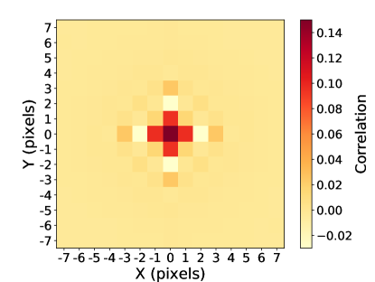
However, the resampling process to produce the HSC coadds induces pixel-to-pixel correlations which do not vary strongly across the sky. We use the cutout blank sky regions to characterize the average noise correlation function, and use the same noise correlation function for all simulations (see Fig. 1), simply rescaling the overall variance to match the estimates from randomly-distributed survey locations. The randomly-distributed survey locations used for this purpose include some areas that do not pass the weak lensing “full depth full color” (FDFC) cut; we account for this mismatch in a later step of the analysis (Section 4.2.1).

The dominant factor that determines the correlated noise patterns due to interpolation to a common pixel grid is simply the interpolation kernel, which is the same everywhere. We have explicitly confirmed that if we consider different patches in the survey, and find the average spatial correlation function of the noise across an entire patch, then each patch gives very similar results. Smaller-scale variation of the noise correlation function is difficult to measure empirically, so we estimated its magnitude on theoretical grounds: for a given point in the coadd, we find the single visits and their corresponding WCS and noise properties. After coadding many noise realizations of the visit, it is possible to calculate the average noise correlation function from the different realizations. Since the dominant correlations are on distance scales of 1 pixel, we focus just on the value of the noise correlation function at that separation, finding that it ranges from 0.08–0.11 in the majority of the area of each patch, though with occasional excursions down to 0.06 or up to 0.13. In Section 5.4, we consider the implications for our shear calibration estimates due to the fact that we have neglected this spatial variation of the noise correlation function.

Figure 1: The noise correlation function as a function of distance, averaged over all the blank sky regions. The color scale is truncated to increase the dynamic range; the correlation is defined such that the pixel at $(0,0)$ has a value of 1.

In order to avoid propagating the full noise covariance to the coadd, the HSC pipeline scales the variance values stored with the coadded image such that the measured variance of the quantity (signal/standard deviation) is 1 for pixels identified as noise pixels containing no astrophysical object. In principle the goal is that photometry algorithms would then report approximately the same uncertainty that they would measure if the full covariance and true variance were available, though this is unlikely to be true in detail. The scaled variance is also used when measuring shapes and estimating the shape measurement uncertainty, and hence it must be included in our simulations so we can reverse its effect while accounting more rigorously for the effects of correlated noise. The simulation estimates of variances (of fluxes etc.) must be similarly rescaled using the same rescaling factors as in the real data in order for the catalog-level outputs in data and simulations to be comparable.

3.3 Galaxy models

Multiple different parent samples as described below and summarized in Table 1 were used to make several sets of simulations. These different simulation sets were used to explore different issues.

Table 1: Summary of different parent galaxy samples from Section 3.3, including how the samples were selected; how the galaxy model is represented in the simulations; whether nearby galaxies are included in the simulations or not; whether the 7% of the objects in the sample that have possible image artifacts, poor masking, or bad parametric fits are eliminated; and whether or not the HSC pipeline analysis included detection and deblending. See the relevant section listed in the table for more detail. The majority of our analysis uses parent sample 4, with the other 3 only used to understand the sensitivity to various steps in the analysis.

Name	Section	Selection	Galaxy model	Includes nearby	Marginal	HSC pipeline
				structure?	cuts?	analysis
1	3.3.1	HST selection & cuts & deblending	Image	No	Yes	No detection, deblending
2	3.3.2	HST selection & cuts & deblending	Parametric fit	No	Yes	No detection, deblending
3	3.3.3	HST selection & cuts	Image	Partially	No	Detection, deblending
4	3.3.4	HSC selection	Image	Yes	No	Detection, deblending

In all cases, the COSMOS survey is the source of the parent samples. The COSMOS HST Advanced Camera for Surveys (ACS) field (Koekemoer et al., 2007; Scoville et al., 2007a, b) is a contiguous 1.64 degrees² region that was tiled by 575 adjacent and slightly overlapping pointings of the ACS Wide Field Channel. Images were taken through the wide F814W filter (‘Broad I’). In this paper we use the ‘unrotated’ images (as opposed to North up) to avoid rotating the original frame of the PSF. The raw images were corrected for charge transfer inefficiency (CTI) following Massey et al. (2010). Image registration, geometric distortion, sky subtraction, cosmic ray rejection and the final combination of the dithered images were performed by the multidrizzle algorithm (Koekemoer et al., 2002). As described in Rhodes et al. (2007), a finer pixel scale of $0.03\arcsec/$pix was used for the final co-added images. The catalog of object detections was constructed following the methodology outlined in Leauthaud et al. (2007) and then matched to the COSMOS photometric redshift catalogue presented in Ilbert et al. (2009).

3.3.1 Deblended postage stamps

The parent sample called ‘1’ in Table 1 was constructed in the same way as the parent sample used for the GREAT3 challenge (Mandelbaum et al., 2014), following Mandelbaum et al. (2012), but with a deeper magnitude limit of F814W$<25.2$. In short, the object selection proceeded from a catalog of objects in the COSMOS survey described at the start of this subsection. In addition to the magnitude cut, a set of selection criteria were imposed:

• MU_CLASS $=1$: This requirement uses the relationship between the object magnitude and peak surface brightness to select galaxies, and to reject stars and junk objects such as residual cosmic rays (Leauthaud et al., 2007).

• CLEAN $=1$: This cut eliminates galaxies with defects due to very nearby bright stars, or other similar issues.

• GOOD_ZPHOT_SOURCE $=1$: This cut requires that there be a good photometric redshift in the COSMOS catalog. More specifically, it requires that there is a match between the detection in the HST imaging and the Subaru $BVIz$ ground-based catalog, that the object not fall within a mask in the ground-based imaging, and that the estimated photometric redshift lies in the range $[0,9]$.

A random subsample of these galaxies was selected to reduce the size of the dataset.

For each of these galaxies, the size of the postage stamp was estimated based on the object size as described in Mandelbaum et al. (2012). If this postage stamp size causes the postage stamp to hit the CCD edge, then the galaxy is eliminated. Consequently, the probability of a galaxy in our parent sample having a postage stamp is a weak function of the observed galaxy size, specifically the FLUX_RADIUS determined by SExtractor (Bertin & Arnouts, 1996). Fortunately, it is possible to reweight the sample probabilistically to counteract this selection effect when making simulations.

Finally, pixels flagged by SExtractor as belonging to some other object were masked with a correlated noise field. This means that we rely on the entire object detection, selection, and deblending process in COSMOS when creating the sample. The last of these is questionable in the context of simulating a ground-based survey, because it may be possible to deblend two objects in space-based imaging that would always be detected as just a single object from the ground. Thus, in the simulations, the system appears as two distinct objects, whereas in the HSC data it would always appear as just one due to unrecognized blending. In this case, if the two objects are at the same redshift, then the right thing to do when making simulations to test shear recovery is to simply include it as a single system. If they are at different redshifts, then their true shears differ and it is unclear how to interpret the inferred calibration biases from simulations that assume they are at the same redshift.

This parent galaxy sample is publicly available and is set up for easy use with GalSim. The GalSim COSMOSCatalog class handles the needed numerical manipulations such as removal of the HST PSF, shearing in Fourier space, convolving with the target PSF, and resampling to the target pixel scale in a way that is transparent to the user. This process was numerically validated to the level needed to test shear at the level needed for Stage IV dark energy surveys, as described in Rowe et al. (2015).

The COSMOSCatalog class also optionally imposes cuts on the catalog to eliminate objects with possibly problematic image postage stamps (e.g., contaminated by image artifacts) or parametric fits using a keyword exclusion_level=‘marginal’. This cut eliminates $\sim$7% of the objects, and was used for sample 1. Many of the problematic postage stamps have issues with masking of nearby objects, which is the primary motivation for using this cut even though the sample 1 simulations use the image rather than a parametric model.

However, it was realized in the process of carrying out the work in this paper that imposing the GOOD_ZPHOT_SOURCE $=1$ selection criterion had the unintended consequence of excluding galaxies with close neighbors. We find that this flag induces a separation-dependent pair exclusion for galaxy pairs closer than 2.4″, down to 0.9″where all nearby galaxy pairs in which both galaxies are above the detection limit are effectively removed by this cut. There are several possible reasons for this problem: poor deblending in the ground-based catalog, photometric redshift failures preferentially for close pairs (though this explanation is disfavored by the findings of Kobayashi et al. 2015), or over-deblending in the HST image processing. The potential exclusion of close galaxy pairs in the parent sample used for our simulations may be problematic for the purpose of this work, leading to an under-representation of the population of blended galaxies for which both objects are above the detection limit. For objects that are too close to be distinguished, the fact that both are not in our catalogue is actually a positive side effect from this selection criterion; we only want that unrecognized blend system consisting of the two galaxies together to appear in simulations once, not twice (which would lead to double-counting). However, while there are some advantages and disadvantages to this selection criterion, the desire for more control over how galaxies are selected led us to redefine a parent sample defined based on actual HSC detections in the COSMOS field (parent sample 4, described below).

3.3.2 Parametric fits

Parent sample 2 is essentially the same as sample 1, except that instead of using the HST images as the basis for the image simulations, we use a set of Sérsic fits to those HST images. The fitting methodology is the same as was used for the GREAT3 challenge (described in detail in Mandelbaum et al. 2014). In short, galaxies were fit to a single Sérsic profile and to a sum of a bulge and disk component with fixed Sérsic indices. For those galaxies for which a two-component fit was statistically preferable as determined by its having a lower median absolute deviation (or MAD), that fit was used, while for the others ($\sim 70$% of the sample) the single Sérsic fit was used. The GalSim COSMOSCatalog class is set up to interchangeably use the parametric fits that are publicly distributed with this sample (same URL as for sample 1); a single keyword argument determines whether the HST image or the parametric fit is used. Because of this, the only difference between simulations with sample 1 and sample 2 is the inclusion of parametric (sample 2) or fully realistic (sample 1) galaxy morphology.

3.3.3 Postage stamps without deblending

Parent sample 3 is very similar to parent sample 1, but in this case, the nearby objects detected based on the SExtractor deblender were not masked with a correlated noise field. Hence sample 3 includes not only realistic galaxy morphology, but also the impact of nearby structure and unrecognized blends. In Table 1, this sample is listed as ‘partially’ including the effects of nearby structure. The reason this is partial rather than complete is that some of the postage stamps used were still relatively small – small enough that they do not cover the entire postage stamp area in the simulations. In principle this is unlikely to be a problem, because the outer edges contain objects that would always be securely detected and deblended in the ground-based survey, but we cannot a priori rule out low-level issues due to these small-area postage stamps.

Because many of the image artifacts that are flagged with the ‘marginal’ cut relate to masking of nearby objects, and those objects are deliberately not masked for sample 3, the ‘marginal’ cut was not used for this sample.

Note that the comments about nearby galaxy pairs at the end of Section 3.3.1 for parent sample 1 also apply here, since parent sample 3 was selected in the same way as parent sample 1.

3.3.4 Final parent sample

Parent sample 4 is the one that we use for the majority of the results in this paper. Its design was intended to serve several purposes that improve upon the pre-existing samples 1–3:

• To avoid selection effects due to the selection criteria for samples 1–3 described in Section 3.3.1, we select the galaxies based on HSC detections with minimal constraints, rather than selecting them based on HST detections with additional constraining selection criteria. The process of selecting based on HSC will be described below.

• We do not deblend based on the HST images. Instead, the images are fed into the simulation software and used to make simulations, and we rely exclusively on the HSC deblender (as for real analysis of HSC data, and simulations with parent sample 3).

• We use the real HST galaxy images (as in samples 1 and 3), not parametric fits (as in sample 2), to include realistic galaxy morphologies.

• The postage stamp sizes are chosen such that all structure around the central detection out to the edge of the simulated postage stamps is included in the simulations.

This sample has been publicly distributed as part of an HSC survey incremental data release.

Our selection of parent sample objects begins with three HSC Wide-depth coadds in the COSMOS region that were described in Aihara et al. (2018b). These coadds were produced from the HSC Deep layer data, and have fewer exposures than in a typical Wide layer coadd due to the differences in exposure times. Exposures with different seeing values were used to create Wide-depth stacks with effective seeing better than, around the median of, and worse than the HSC Wide layer on average. These stacks have seeing values of 0.5″, 0.7″, and 1.0″, as described in Section 3.8 of Aihara et al. (2018b).

For each of the three coadds, we apply the conservative bright object mask described in Mandelbaum et al. (2018) (not the later version described in Coupon et al. 2018). We then identify all HSC galaxy detections satisfying the following conditions: basic flag cuts for object detection, measurement, and star/galaxy classification as given in the top section of Table 4 in Mandelbaum et al. (2018), followed by a loose cut on magnitude at $i<25.2$ in the HSC imaging. There is no way to impose the weak lensing full depth and full color (FDFC) cut described in Mandelbaum et al. (2018), because of the way these coadds were produced. The justification for this magnitude cut is that scatter in the magnitudes between detections of the same object in the different coadds is large enough that at $2\sigma$, some objects brighter than $i=24.5$ (our limit used for the shear catalog in the data) might actually come from COSMOS objects with F814W$\approx 25.2$. We do not want to apply a stricter magnitude cut, because then we would miss some of the faint objects that may be scattering into our sample in reality. We applied no resolution or S/N cut because we found that there was no reasonable cut that would avoid cutting into the sample of objects in our shear catalog. Fortunately, our magnitude cut is sufficient to remove a large amount of junk detections at very low S/N that would never be used for science, so that we are not resimulating large samples of useless objects.

After imposing these cuts, the locations of these HSC detections are compared with the masks on the HST COSMOS images, and any locations that are masked or are outside the HST COSMOS imaging area get removed. The locations of the remaining detections will be used as the center of the parent sample postage stamps, regardless of whether or not there is a COSMOS detection near that point.

The sizes of the postage stamps are determined based on the following criteria: the minimum postage stamp size is such that the postage stamps cover the entire area of the postage stamps in the simulations, i.e., $64\times 0.168$″ in length. Given the 0.03″ pixel scale for the resampled COSMOS images, our minimum postage stamp size is $380\times 380$. For each galaxy, we use the following formula to determine the nominal postage stamp size needed to contain the galaxy light: ideal stamp width is $12\times r_{\text{det}}^{\text{(HSC)}}$, where the radius here is the observed (PSF-convolved) determinant radius of the HSC detection. If that ideal width is less than 380, we use 380. If the ideal width exceeds 1000, we discard the object from our parent sample. Finally, if the calculated postage stamp size causes the image to overlap a CCD edge, we also discard it. This final cut results in a slightly non-representative distribution of galaxy sizes in the parent sample, with the probability of inclusion in the sample varying by approximately 12 per cent across the full range of galaxy sizes in the sample. However, when randomly drawing from the parent sample, we probabilistically reweight the sample to cancel out this selection effect.

Because of our arbitrary choice of postage stamp sizes, it is entirely possible that some neighboring objects in the postage stamp (not the central one) will be cut off by the postage stamp edges. Fortunately these objects are reasonably far (at least $5$″) from the center of the simulated postage stamps, so in general those detections are being discarded anyway.

While we did not require an HST COSMOS detection matching the locations of these postage stamps, we do cross-match against the COSMOS catalog to identify the nearest COSMOS detection. The purpose of this matching process is to define HST PSF models for all the galaxies, so that GalSim can remove it as the first part of the simulation process.

The outcome of the above process is a set of three parent samples for the three seeing ranges, assembled completely independently, though in practice they have a large fraction of objects in common. In the simulation scripts, we use a different parent sample for each subfield depending on the seeing value in that subfield. For PSF model FWHM values in the ranges $<0.6$″, $[0.6\arcsec,0.85\arcsec]$, $>0.85$″, we use the parent samples defined using the coadds that have seeing better than, around the median of, and worse than the HSC Wide layer. Given the seeing distribution for the galaxies in our shape catalog (Mandelbaum et al., 2018), in practice we almost exclusively use the first two parent samples.

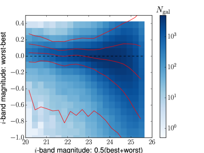
The three parent samples contain 216426, 199461, and 184217 objects as we go from best to worst seeing. There is a significant overlap in the RA/dec positions, but we do see seeing-dependent blending effects. An illustration is shown in Fig. 2. Here we identify matches within 1″ in the best-seeing and worst-seeing coadds, then show a 2D histogram of the difference in magnitudes for those objects as a function of the magnitude in the best-seeing coadds. As shown, there is substantial skew towards negative $\Delta$mag, meaning that the objects appear brighter in the worse-seeing coadds than in the best-seeing coadds. This could result from unrecognized blends in the worse-seeing coadds that are properly recognized and deblended in the best-seeing coadds.

Figure 2: The logarithmic color-scale shows a 2D histogram of $\Delta$mag (the difference in observed magnitude in the worst-seeing coadds vs. the best-seeing coadds for objects detected in both) as a function of the average of the observed magnitudes in the worst- and best-seeing coadds. The five red lines show the $(5,16,50,84,95)$ percentile values of $\Delta$mag, while the dashed black line shows the ideal value of 0. The coherent skew towards negative values indicates that a subset of the galaxies in the worst-seeing coadd appear consistently brighter than the same galaxies in the best-seeing coadd, due to unrecognized blending effects.

While we believe the procedure in this subsubsection is a more principled way to create the parent samples for these simulations, ultimately the justification of this procedure rests on what we find when analyzing the simulations. That is, the distributions of simulated galaxy properties (as measured by the HSC pipeline after running the object detection, deblending, and measurement routines) should match those in the real shape catalog. In addition, we have no process for addressing systematic errors due to unrecognized blends at different redshifts, since our simulations assume they are at the same redshift.

3.3.5 Impact of different parent sample selection

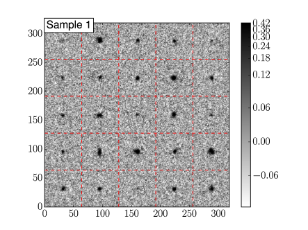
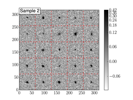
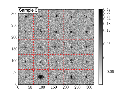
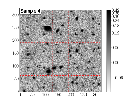
In Section 5.7 we will quantify the impact of using these different parent samples on estimated shear biases. For now, we give a visual demonstration of the impact of different parent samples by showing cutouts from the simulations with different parent samples in Figure 3. As shown, for parent samples 1-2, the simulated postage stamps just have a single object by design. For sample 3, there are nearby objects, but nothing near the edges of postage stamps, because the typical postage stamp size in COSMOS covered a smaller spatial extent than these postage stamps. However, the nearby structure should be the most important at affecting the measured properties of the central object. Finally, by design the sample 4 images have nearby structures included out to the edge of the postage stamps, in some cases artificially truncated by the postage stamp edges. In all cases it is only the central object in the postage stamp that is used for the simulation analysis.

A final difference between the simulations with the different parent samples is that samples 1–3 were produced with a S/N$<80$ cut, to focus on the low-S/N regime where shear calibration varies strongly, whereas sample 4 simulations do not have this cut. This cut could not be applied in practice because sometimes faint objects had nearby bright ones, and the bright ones contributed to the S/N estimate that was computed on the fly while producing the simulations (without deblending), so the S/N cut would have led to the exclusion of galaxies well below the cut value. Because of the S/N cut being present in some simulation sets and not others, the figures that characterize and compare galaxy populations have a S/N$<80$ cut imposed on all samples (to enable fair comparison across simulation samples), but the shear calibration results that use sample 4 go above S/N$=80$.

Figure 3: Example simulated images for simulations with the four parent samples as labeled on each plot. All images have the same zero points, and the symlog color scales are the same on each panel. For the purpose of illustration we have chosen images with the same PSF model. Dashed red lines show the artificial boundaries between individual postage stamps; we have shown a $5\times 5$ postage stamp region ($320\times 320$ pixels) out of the simulated image composed of $100\times 100$ postage stamps. Note that the color-scale is saturated in some places for sample 4 simulations, because some of the stamps include bright stars that happen to lie close enough to our central objects that they are included in the simulations. The sample 3 and sample 4 images look quite different from each other, despite the choice to not mask nearby objects in either sample, because sample 4 images were created from larger postage stamps (sufficiently large that they include some irrelevant structures that would never be blended with the central objects). We demonstrate later in this work that the measured properties of the central galaxies in the postage stamps and their shear calibration biases are very similar in samples 3 and 4 (Fig. 17).

4 Analysis

In this section we describe how the simulations were analyzed. They were run through the HSC pipeline followed by a series of analysis routines aimed at measuring shear calibration biases.

4.1 HSC pipeline

The HSC pipeline, as described in Bosch et al. (2018), is being developed for the Large Synoptic Survey Telescope (LSST; Axelrod et al. 2010; Jurić et al. 2015). Because of the setup of the simulations, we did not need to run the full HSC pipeline. We assumed perfect knowledge of the PSF, background, and astrometric and photometric calibration. The first step in processing the simulations was to define a list of objects and their associated pixels. The list of all the pixels defined for a particular object is called a footprint. When processing simulations made with samples 1 and 2, no explicit detection was performed because there was only one object per postage stamp. Instead, we used the stamp center as the peak and assigned all pixels from the stamp to the footprint. This resulted in larger footprints for these samples than in the real data, but had little impact on the actual measurements. The noise in these images was found by taking the variance of pixels around the borders of the postage stamps.

For simulations produced using samples 3 and 4, more than one object was present in most postage stamps. We therefore ran the detection algorithm to identify sources. This algorithm performs a maximum likelihood analysis to detect all pixels with a 5$\sigma$ threshold, using a Gaussian smoothing filter matched to the size of the PSF. Connected pixel regions above threshold are identified as the footprint and sources are defined as peaks within each footprint. If more than one peak per footprint was found, we ran the deblending algorithm, which apportions the flux to the different objects. In the event that no object was detected in a postage stamp, we artificially inserted one with the peak at the center of stamp. Because objects could be near an edge in these samples, the noise for these was calculated by taking the variance of all pixels not part of a detected footprint. The final step was to run the full suite of measurement algorithms on the deblended images. Table 1 includes a summary of the key difference between how the simulations with the different parent samples were analyzed in the HSC pipeline (i.e., was detection and deblending done or not).

The main differences between the coadded $i$-band data and simulations are:

• The presence of artifacts like cosmic rays in the data.

• In the data, images are resampled and then coadded. In the simulations, we generate a single-band image and account for the impact of resampling on average by adding correlations to the noise as described in Section 3.2.

• Object detection is done on the data by merging peaks from multiple bands. This can lead to more spurious objects when making cuts on $i$-band quantities; hence, in the data we have a multi-band detection requirement, which is irrelevant in the single-band simulations.

• The number of objects in a blend is typically smaller in the simulations than in the data. This difference is potentially relevant because the performance of the deblender has been shown to be worse as more objects are included. However, the number of many-object blends in the data is enhanced by the presence of bright stars and galaxies; in some cases, none of those will be deblended into systems that have any lensing-selected galaxies. As a result, this difference may not result in the lensing-selected samples in simulations and data having any important differences.

• The simulations only contain galaxies at the centers of postage stamps. For samples 3 and 4, images of stars could appear on galaxy outskirts, not at the centers of postage stamps; for samples 1 and 2, no stars will appear anywhere.

• The data contains relative astrometric offsets between visits slightly blurring the PSF relative to the model. As shown in Mandelbaum et al. (2018), the impact on the coadded PSFs is negligible, which justifies our ignoring this effect in this work.

These differences require us to impose slightly different cuts in order to get consistent samples between the data and simulations, as described below.

4.2 Higher level analysis software framework

In order to ensure consistency in the treatment of simulation outputs, the results presented in the remainder of this work rely on a common analysis framework. This framework is tasked in particular with ensuring that simulations match the observed data in terms of noise variance and PSF size, through a reweighting scheme described in Section 4.2.1. It also provides a unified set of routines to transparently handle simulations and data, and apply various cuts and selection criteria in a consistent fashion.

The simulations are specifically designed to include $90^{\circ}$ rotated pairs of galaxies which can be used to nearly cancel out shape noise. This feature is particularly useful for our estimation of shape measurement errors, as described below, and to reduce statistical errors on shear biases, enabling them to be robustly quantified with fewer simulations. By keeping track of the members of each pairs, the analysis framework provides several options to apply this cancellation or not. In all cases, a basic set of flag cuts are imposed. These are a subset of the cuts in the ‘Basic flag cuts’ section of table 4 of Mandelbaum et al. (2018) for the shear catalog, where the cuts that are omitted are unnecessary in the simulations due to how they were produced. Specifically, for simulations (which are single-band images with no image artifacts), we only need the cuts on idetect_is_primary, iflags_badcentroid, icentroid_sdss_flags, iclassification_extendedness, and ishape_hsm_regauss_sigma. We also impose a cut specific to the simulations, requiring that the detection nearest the center of the postage stamp have a centroid that is a maximum of 5 pixels from the center; this cut was empirically determined as a way of eliminating stamps where the detection nearest the center was not the intended central object.

After the imposition of those flag cuts, further selection criteria in the ‘Cuts on object properties’ section of table 4 of Mandelbaum et al. (2018) are imposed based on whether shape noise cancellation is desired or not. Without shape noise cancellation, all galaxies passing a given set of cuts are retained. With shape noise cancellation, pairs where one member has not been detected by the HSC pipeline are first discarded, and of the remaining pairs, only those in which a randomly selected member passes the specified set of cuts are retained, as to avoid selection bias entirely.

4.2.1 Different simulation and data versions

The simulations described in this work were produced using PSF and sky variance levels corresponding to an earlier version of the shape catalog compared to the one used for science and characterized in Mandelbaum et al. (2018). The primary differences are that the catalog from Mandelbaum et al. (2018) includes data that were taken later, but has regions that do not correspond to full depth in all five bands removed. As a result, the simulations have some subfields with much higher noise variance than in the final shape catalog (Fig. 4).

To address this issue, we included in our software framework an option to separately reweight the simulations to match the distributions of sky variance and PSF FWHM as in the final shape catalog. This results in a small fraction of the subfields being excluded altogether, while many others have weights that differ from 1. The reweighting does not account for differences in PSF shape or higher order moments; however, these should have a relatively smaller effect on the observed galaxy properties in the simulations and data compared to the sky noise level and PSF FWHM.

Figure 4: Distribution of the noise variance, for each field and for simulations vs. data (S16A), after reweighting the simulations to match the imaging conditions in the data. The top two rows are for each field individually, while the bottom left is for the average over all fields; all panels show reasonable consistency between simulations and data. Finally, the bottom middle panel shows the average over all fields, without reweighting to account for differences in imaging conditions.

Figure 5: Distribution of the PSF FWHM for each field in HSC and for simulations vs. data (S16A), after reweighting the simulations to match the imaging conditions in the data. The top two rows are for each field individually, while the bottom left is for the average over all fields; all panels show reasonable consistency between simulations and data. Finally, the bottom middle panel shows the average over all fields, without reweighting to account for differences in imaging conditions. The weighted mean PSF FWHM values are given on the plot and indicated with vertical lines.

Figure 6: Distribution of the per-component PSF ellipticity, for each field in HSC and for simulations vs. data. The panels are defined in the same way as in Fig. 5.

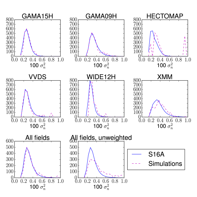
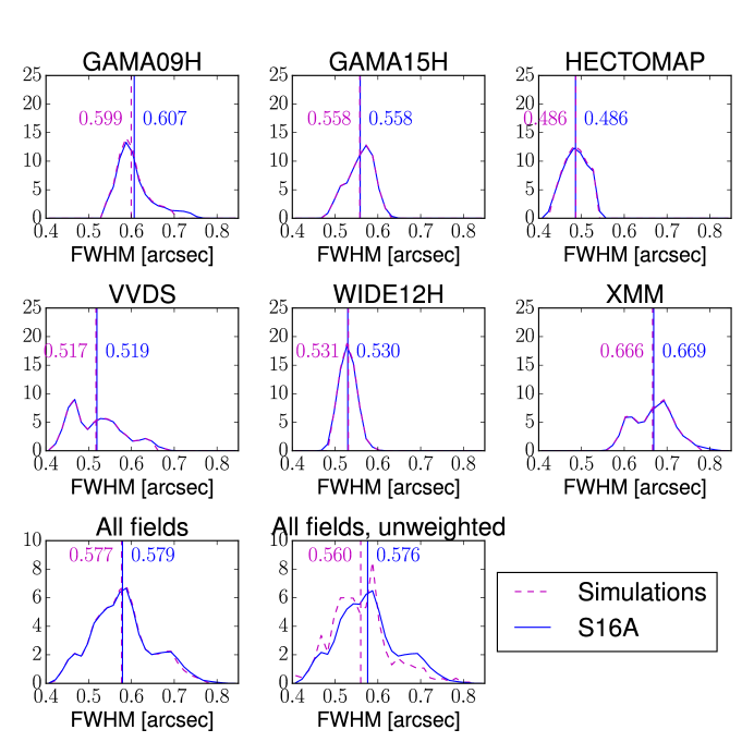
As shown in Figure 5, after reweighting, the distributions of PSF FWHM in simulations and data are well-matched. The match will not be perfect because of the fact that our simulations have the same PSF within each subfield, and hence the finite number of subfields is a limitation in matching the full joint distribution of PSF FWHM and noise variance (Fig. 4). Figure 5 shows that the means and overall shape of the PSF size distributions in the simulations and data are indeed well-matched; for the survey overall, the mean PSF sizes in the data and simulations agree to within 0.3 per cent, an order of magnitude better than without the reweighting.

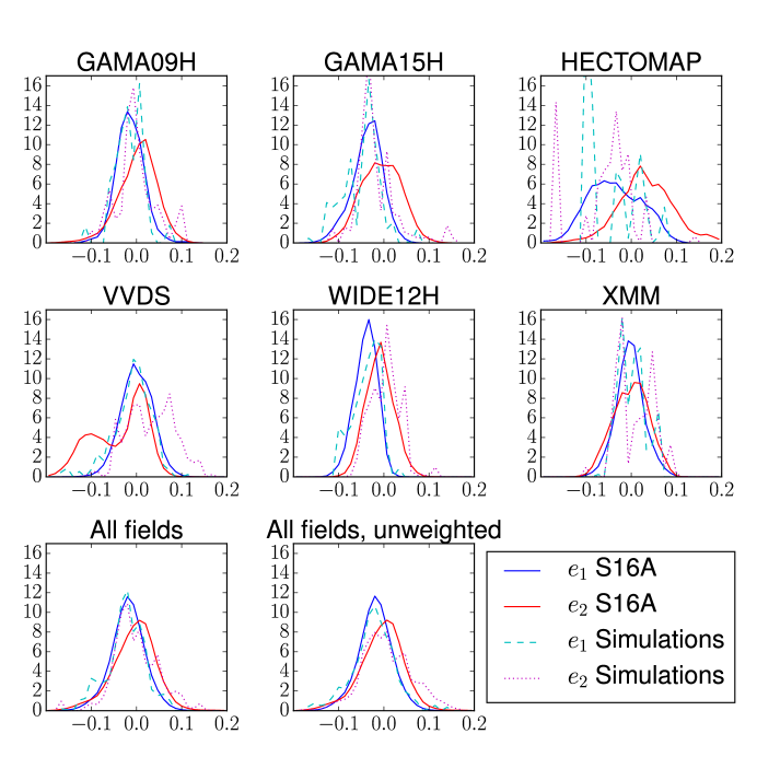
We have not made any attempt to reweight the simulations to match the distribution of PSF ellipticity in the final shear catalog, and hence some mismatch is seen as in Figure 6. However, the primary reason to do the reweighting is to match the empirical distribution of object properties that determine shear calibration (such as S/N and resolution factor). Since PSF ellipticity is not a dominant driver of the object S/N or resolution, this mismatch between data and simulations is acceptable.

4.3 Shape measurement error

In order to apply optimal weighting to the galaxy shapes when inferring ensemble shear, we need to understand the shape measurement errors $\sigma_{e}$ as a function of galaxy properties. The re-Gaussianization algorithm includes a naive formula for shape measurement error, but this formula has been shown to be incorrect by at least tens of percent in SDSS (Reyes et al., 2012), and does not account for correlated noise as in the HSC coadds, so we use the simulations in this paper to make a more accurate estimate that will enable more optimal weighting.

The method adopted here relies on the fact that the simulations have pairs of galaxies that are rotated by $90^{\circ}$ with respect to each other, but with nearly independent realizations of the noise field. The mathematical basis of our $\sigma_{e}$ estimates is given in Appendix A.

Our expectation is that to lowest order, the shape measurement error will depend on the detection signal-to-noise ratio S/N and the resolution factor $R_{2}$. For that reason, we define a sliding window in that 2D parameter space, and estimate $\sigma_{e}$ as a function of position in that plane. We also confirm that the 2D relationship defined in this way, $\sigma_{e}(\text{S/N},R_{2})$, does not depend significantly on other parameters such as cuts on the magnitude or observing conditions (which primarily shift around the distribution of the galaxies in that 2D plane without modifying the $\sigma_{e}(\text{S/N},R_{2})$ relation).

4.4 Intrinsic shape dispersion

The per-component intrinsic shape dispersion, $e_{\text{rms}}$, is generally estimated from the shapes in the real data with galaxies indexed $i$ as follows:

$$e_{\text{rms}}=\sqrt{\frac{\sum_{i}w_{i}\left(e_{i,1}^{2}+e_{i,2}^{2}-2\sigma_{e}^{2}(\text{S/N}_{i},R_{2,i})\right)}{2\sum_{i}w_{i}}}.$$ (3)

This is effectively a weighted shape dispersion with the measurement error subtracted off in quadrature. The main assumptions behind this equation are (1) that the measurement errors are correctly estimated, and (2) that the measurement errors are independent of the shape noise. We rely on the calculation described in Section 4.3 to ensure the reliability of the first assumption. For (2), while the magnitude of the measurement errors have a very slight dependence on the galaxy ellipticity, the correlation between those errors is too mild to invalidate Equation (3). This equation is valid in the limit that the observed shape dispersion can be modeled as the convolution of the intrinsic shape dispersion and that due to measurement error; but no assumption is made about their functional forms. We have explicitly tested its validity using simulations with parametric galaxy models on a grid of S/N and resolution factor values, and found that for S/N$\sim$20, the above assumptions are valid for galaxies with $|e|$ values below the 90th percentile, while the remaining galaxies exhibit low-level anticorrelations between intrinsic shape and measurement error. For S/N$>50$ it is valid for essentially the entire sample. Based on our process of forward-modeling this effect and testing the validity of Eq. 3, we estimate that the failure of its assumptions leads to a $\sim 2$% bias in the estimated $e_{\text{RMS}}$ for objects with S/N$\sim$20, below which there are very few galaxies in our sample. Given this low bias that is reduced rapidly at higher S/N, along with the fact that the resulting shear biases (due to incorrect shear responsivity) will be directly calibrated out using the simulations, we rely on Eq. 3 for our analysis despite its limitations.

The weights in Equation 3 are defined in Eq. (6). In principle this is circular, since $e_{\text{rms}}$ appears in the weights. To address this problem, we use an estimate from SDSS for $e_{\text{rms}}$ in the weights (Reyes et al., 2012), estimate $e_{\text{rms}}$ using those approximate weights, then use that $e_{\text{rms}}$ estimate to update the weights, and confirm that if we iteratively try to re-estimate $e_{\text{rms}}$ there are no significant changes.

As for $\sigma_{e}$, we estimate the intrinsic shape dispersion as a function of S/N and $R_{2}$.

4.5 Shear calibration and additive bias

The detailed process for estimating shears is given in appendix 3 of Mandelbaum et al. (2018). Here we summarize the key equations, where the relevant quantities for shear estimation are as follows:

• Distortions $e_{1}$, $e_{2}$ in pixel coordinates.

• Shape weights $w$: These are defined as inverse variance weights summing in quadrature the measurement errors (Section 4.3) and intrinsic shape dispersion (Section 4.4).

• Intrinsic shape dispersion per component $e_{\text{rms}}$: These are defined as in Section 4.4.

• Multiplicative bias $m$ averaged over components. These biases are determined through the procedure described in this section. Thus, for the initial calculation in this section, we set $m=0$. When testing the efficacy of our calibration bias corrections, we later use the $m$ values determined from the simulations.

• Additive biases $c_{1}$, $c_{2}$: These are set to 0 for the initial calculation, and then determined from the simulations as described below.

The ensemble shear per component can be determined using all galaxies indexed $i$ in a given subfield $j$. The ensemble average distortion is an estimator for the shear $g$,

$$(\hat{g}_{\mathrm{1}},\hat{g}_{\mathrm{2}})=\frac{1}{2\cal R}\langle(e_{\mathrm{1}},e_{\mathrm{2}})\rangle,$$ (4)

where the ‘shear responsivity’ ${\cal R}$ represents the response of the distortion to a small shear (Kaiser et al., 1995; Bernstein & Jarvis, 2002); ${\cal R}\approx 1-e_{\mathrm{rms}}^{2}$, where $e_{\mathrm{rms}}$ is the RMS intrinsic distortion per component. Hence we begin by empirically estimating the responsivity for the source population in that subfield as

$${\cal R}_{j}=1-\frac{\sum_{i}w_{i}e_{\text{rms},i}^{2}}{\sum_{i}w_{i}}.$$ (5)

The lensing weights $w_{i}$ are defined as

$$w_{i}=\frac{1}{\sigma_{e,i}^{2}+e_{\text{rms},i}^{2}}$$ (6)

where $\sigma_{e,i}$ is the estimate of the per-component shape measurement error due to pixel noise for object $i$ (with a strong dependence on object properties such as S/N) and $e_{\text{rms},i}$ is the per-component RMS intrinsic shape dispersion. Note that in general that quantity is defined for the ensemble; the $i$ is meant to indicate that we determine and model its slow variation with object properties.

We can use the catalog estimates of calibration bias $m_{i}$ to derive an ensemble estimate for the calibration bias for our sample:

$$\hat{m}_{j}=\frac{\sum_{i}w_{i}m_{i}}{\sum_{i}w_{i}}$$ (7)

In the initial calculation, $\hat{m}_{j}=0$; it is only nonzero after we have determined an initial set of calibration corrections. Likewise, the additive correction term can be derived from a weighted sum in each component $k$,

$$\hat{c}_{j,k}=\frac{\sum_{i}w_{i}c_{i,j,k}}{\sum_{i}w_{i}},$$ (8)

which will be zero in our initial shear estimation.

Finally, these can be combined with the standard average over tangential shear estimates to get the stacked shear estimator per component $k$

$$\hat{g}_{j,k}=\frac{\sum_{i}w_{i}e_{i,k}}{2{\cal R}_{j}(1+\hat{m}_{j})\sum_{i}w_{i}}-\frac{\hat{c}_{j,k}}{1+\hat{m}_{j}}.$$ (9)

At the end of this process, we have the following quantities for each subfield $j$:

1. Estimated shear $\hat{g}_{j,k}$ per component.

2. True shear $g_{j,k}$ per component.

3. PSF shear $g_{j,k}^{\text{(PSF)}}$.

4. A weight for each subfield, $w_{j}$. For this purpose, we use the weights that are defined to force the simulations to match the observing conditions in the data as defined in Section 4.2.1, but do not do any inverse variance weighting since the uncertainties in the ensemble shear estimates do not vary strongly by subfield.

Our model for the per-object systematics is that a given object has a property-dependent multiplicative bias $m_{i,k}$ and a fraction of the additive PSF anisotropy that leaks into the ensemble shear estimates, $a_{i,k}$, giving an additive term that depends on the galaxy properties and the PSF that convolves it, $c_{i,j,k}\equiv a_{i,k}g_{j,k}^{\text{(PSF)}}$. As for $\sigma_{e}$, we define a sliding window in S/N and $R_{2}$ values, and then carry out a weighted linear regression to the shear estimates averaged within bins in that 2D plane to estimate $m_{i,k}$ and $a_{i,k}$:

$$\hat{g}_{j,k}-g_{j,k}=m_{i,k}g_{j,k}+a_{i,k}g_{j,k}^{\text{(PSF)}}.$$ (10)

We then take the mean of the two shear components to estimate the $m_{i}$ and $a_{i}$ values that are relevant for a real lensing analysis (where the shear components are measured in the tangential/radial coordinate system, effectively averaging over the components in the pixel basis).

Finally, to confirm the efficacy of our calibration corrections in our shear estimator in Equation (9), we carry out a round-trip exercise wherein shear estimation is done in the simulations using the simulation-defined $m_{i}$ and $c_{i,k}$ values based on each object’s S/N and $R_{2}$ values. While this should trivially provide us with unbiased shear estimates, we can split the simulations by observational conditions and other properties such as the apparent magnitude or photometric redshift, and confirm that the calibration corrections are still suitable for the kinds of subsamples we encounter when measuring shear in the real data.

4.6 Selection bias

Selection bias is an effect wherein quantities used to select or weight the galaxies entering the lensing analysis depend on the galaxy shape, and therefore the probability of a galaxy entering the sample (or the weight assigned to a galaxy in the sample) depends on its alignment with respect to the shear direction or the PSF anisotropy direction. This results in a violation of the assumption that galaxy intrinsic shapes are isotropically oriented. If the selection probability or weight depends on the shear, there will be a multiplicative bias, whereas if they depend on the PSF shape, there will be an additive bias.

For this discussion, we will refer generically to quantities $X$ used for selection or weighting; as described in Mandelbaum et al. (2018), the primary quantities used for selection are $R_{2}$, $i$-band cmodel magnitude, and $i$-band cmodel S/N. In addition, there are the weights defined in Eq. (6). Here we treat multiplicative selection biases as causing the observed value of $\hat{X}$ (used for selection or weighting) to deviate from the true one $\hat{X}$ as

$$\Delta X\equiv\hat{X}-X\propto|g|\cos{(2\phi)},$$ (11)

where $|g|$ is the lensing shear magnitude, and $\phi$ is the angle between the galaxy intrinsic shape and the lensing shear. The fact that this is proportional to $|g|$ can be thought of as a Taylor expansion of some potentially more complex function, taken to the $|g|\ll 1$ regime. The $\cos{(2\phi)}$ term comes from basic symmetry considerations. This equation is a generalization of an expression derived for $\Delta R_{2}$ based on the Gaussian approximation in Mandelbaum et al. (2005), in which case the constant of proportionality is uniquely defined and depends on the magnitude of the galaxy intrinsic distortion. However, for the cmodel-related quantities and the weights, which are all derived through complex multi-step analyses, there is no obvious way to derive the constant of proportionality (or even what it depends on) from first principles, so we rely on the simulations to determine this information. The sign of the constant of proportionality determines the sign of the shear bias. A similar equation to Eq. (11) can be written for additive selection biases, using the magnitude of the PSF anisotropy and the angle between the galaxy and PSF shapes.

Below we describe separately how we quantify the edge-related and weight-related types of selection effects so that we can remove the resulting biases in the ensemble shear signals.

4.6.1 Selection bias due to weights

If the weights in Eq. (6) depend on galaxy shape, then even away from the boundaries of the sample, we may get some selection bias due to our use of weighted ensemble averages (referred to as ‘weight bias’ by Fenech Conti et al. 2017). Fortunately, the shear estimation process in the simulations that was outlined in Section 4.5 provides us with a way to estimate this directly. As noted there, when exploiting shape noise cancellation, we only use galaxies appearing in 90^∘ rotated pairs (applying our selection criteria at random to one galaxy in the pair), and we enforce the same weight for galaxies in a pair. However, if we permit the two galaxies in the pair to have different weights as determined by their individual values of S/N and $R_{2}$, then the analysis will have weight bias built into it. We can therefore estimate $m_{\text{wt}}$ and $a_{\text{wt}}$, the multiplicative and additive bias parameters due to weight bias, empirically from the simulations.

4.6.2 Selection bias due to cuts

For galaxies near the edges of our sample, the primary concerns are multiplicative and additive biases due to the quantities used for cuts, $\hat{X}$, depending on the shear as in Eq. (11) or on the magnitude of the PSF anisotropy. Conceptually, the magnitude of the selection bias that we expect depends on two things: the prefactor in front of Eq. (11), which quantifies the strength of the dependence of $\hat{X}$ on the shear or PSF ellipticity; and the fraction of the sample that is close enough to the edge that shear or PSF anisotropy can lead to some coherent $\Delta\langle e_{+}\rangle$ along the shear or PSF anisotropy direction. For a single quantity $\hat{X}$, the relevant expression for $\Delta\langle e_{+}\rangle$ is (Mandelbaum et al., 2005, equation 18)

$$\Delta\langle e_{+}\rangle=\int_{0}^{1}\mathrm{d}|e|\frac{\mathrm{d}^{2}n}{\mathrm{d}|e|\,\mathrm{d}\hat{X}}\big{|}_{\text{edge}}\int_{0}^{\pi}\frac{\mathrm{d}\phi}{\pi}|e|\cos{(2\phi)}\Delta X.$$ (12)

This equation implicitly assumes that we are placing a lower limit on $\hat{X}$; the sign flips for an upper limit. The $\Delta X$ will in general be described by some equation like Eq. (11) that cannot be derived analytically, giving $\Delta X=A(|e|,X_{\text{edge}})|g|\cos{(2\phi)}$. In this equation, $\frac{\mathrm{d}^{2}n}{\mathrm{d}|e|\,\mathrm{d}\hat{X}}\big{|}_{\text{edge}}$ is the joint distribution of distortion magnitude and $\hat{X}$ evaluated at the edge of the sample in $\hat{X}$. For some $\hat{X}$ the joint distributions of distortion magnitude $|e|$ and $\hat{X}$ are effectively independent, so

$$\frac{\mathrm{d}^{2}n}{\mathrm{d}|e|\,\mathrm{d}\hat{X}}\big{|}_{\text{edge}}\equiv p(|e|)p(\hat{X})_{\text{edge}}.$$ (13)

Simplifying Eq. (12), we find

$$\Delta\langle e_{+}\rangle =|g|p(\hat{X})_{\text{edge}}\int_{0}^{1}\mathrm{d}|e|\,|e|p(|e|)A(|e|,X_{\text{edge}})\times$$

$$\qquad\qquad\qquad\qquad\qquad\qquad\int_{0}^{\pi}\frac{\mathrm{d}\phi}{\pi}\cos^{2}{(2\phi)}$$ (14)

$$=\frac{1}{2}|g|p(\hat{X})_{\text{edge}}\int_{0}^{1}\mathrm{d}|e|\,|e|p(|e|)A(|e|,X_{\text{edge}}).$$ (15)

Since the added shear due to a cut on $\hat{X}$ is proportional to the shear itself, we can write this as a multiplicative shear selection bias that depends on the distribution of $\hat{X}$ as

$$m_{\text{sel}}(\hat{X})\propto p(\hat{X})_{\text{edge}}.$$ (16)

We are absorbing the complexity of how $\Delta X$ depends on the galaxy shape and other properties in the constant of proportionality. By a similar formalism,

$$a_{\text{sel}}(\hat{X})\propto p(\hat{X})_{\text{edge}}.$$ (17)

Our approach is to assert these relationships, estimate the factors of proportionality directly in the simulations, and then test whether those factors of proportionality still hold if we change the cuts we apply. In order to estimate the factors of proportionality directly in the simulations, we estimate the shear without imposing shape noise cancellation. In this case, the two galaxies in the $90^{\circ}$ rotated pairs are selected based on their own $\hat{X}$ values, and both additive and multiplicative selection biases should be evident.

Because of our expectation that the selection biases should be directly proportional to $p(\hat{X})_{\text{edge}}$ for each cut quantity $\hat{X}$, we focus on resolution factor and magnitude. As shown in Fig. 8, these two cuts affect the sample quite significantly, so the distribution of both quantities is non-negligible near the edge of the sample. In contrast, the S/N cut removes less than one per cent of the objects passing the other two cuts. Additional cuts given in Mandelbaum et al. (2018), such as on blendedness and multiband S/N, function primarily as junk rejection cuts that remove tiny fractions of the sample, and hence we do not carry out this selection bias analysis for them.

4.7 Outputs

Using the analyses described earlier in this Section, the simulations are used to provide the following catalog entries for use in real lensing analysis:

• Shape weights ishape_hsm_regauss_derived_weight based on the inverse variance (Section 4.3 and 4.4).

• Intrinsic shape dispersion per component ishape_hsm_regauss_derived_rms_e (Section 4.4).

• Multiplicative bias ishape_hsm_regauss_derived_bias_m (Sections 4.5 and 4.6).

• Additive biases ishape_hsm_regauss_derived_bias_c1/c2 (Section 4.5).

In addition, there are ensemble corrections for selection bias due to the cuts placed on S/N, $R_{2}$, and $i$-band magnitude (Section 4.6).

5 Results

In this section we describe the results of analyzing the simulations. For the majority of the results described here, we use parent sample 4 (Table 1 and Section 3.3.4). However, in Section 5.7, we will show results from all parent samples to justify this choice and illustrate the impact of some of the choices of parent sample definition.

Figure 7: Weighted distribution of $i$-band resolution factor (left) and $i$-band cmodel S/N (right) for the HSC S16A shear catalog (top) and the simulations (bottom), shown separately for each field. As shown, the distributions of these two quantities exhibits significant field-dependence, due to the field-dependent variation in observing conditions. The simulations are largely able to reproduce this field-dependence, especially for the resolution factor. This plot shows results for our default simulations, which use parent sample 4 (Table 1 and Section 3.3.4).

Figure 8: Weighted distribution of $i$-band resolution factor (top left), $i$-band cmodel S/N (top right), $i$-band cmodel magnitude (bottom left), and distortion magnitude $|e|$ (bottom right), shown for the HSC S16A shear catalog and the simulations, as an average over the entire survey. The weighted mean values are quoted and shown as vertical lines on the plots. This plot shows results for our default simulations with parent sample 4 (Table 1 and Section 3.3.4), which reproduce the properties of galaxies in the simulations quite well.

Figure 9: The weighted 2D distributions of resolution factor (left), distortion magnitude $|e|$ (middle), and cmodel magnitude (right), vs. the $i$-band cmodel S/N. The grayscale shows the 2D density in the data, while the solid and dashed contours are for the data and simulations, respectively. This plot shows results for our default simulations, which use parent sample 4 (Table 1 and Section 3.3.4).

5.1 Galaxy properties

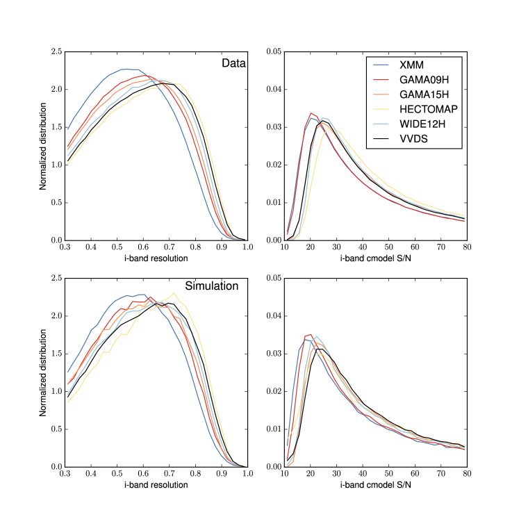
In this section, we compare the distribution of observable galaxy properties that can be inferred from the images in the simulations and data. The first comparison is shown in Figure 7. Here, we compare the weighted distributions of $i$-band resolution factor (left) and $i$-band cmodel S/N (right) for the HSC S16A shear catalog (top) and the simulations (bottom). The distributions have been computed separately for each field, because of the substantial variations in observing conditions between these fields shown in Figures 4 and 5 (however, results averaged across fields are shown in Figure 8). We expect that those differences in observing conditions should lead to differences in the observed properties of galaxies passing our selection criteria, and this figure confirms that that is the case. The differences in PSF FWHM are more striking than the differences in noise variance between the fields. When ranking the fields based on the mean PSF FWHM, they are (from best to worst) HECTOMAP, VVDS, WIDE12H, GAMA15H, GAMA09H, and XMM. As a result, we expect that the average galaxy resolution factor and S/N will be highest for HECTOMAP and lowest for XMM. The results are consistent with those expectations in both the simulations and data.

In contrast, we find (not shown) that the distributions of $i$-band magnitude and distortion magnitude $|e|$ exhibit relatively little field-dependence. The reason for this is that our magnitude cut of $24.5$ in $i$-band corresponds to a S/N that in most cases is substantially higher than the limits in typical weak lensing surveys (and higher than our limit of $10$, which eliminates only a tiny fraction of galaxies that would pass our other cuts). Hence the magnitude distribution does not depend strongly on observing conditions, but for a fixed magnitude, the S/N distribution does depend strongly on observing conditions.

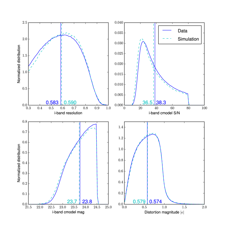
Now that we have confirmed that field-dependent trends in galaxy properties are consistent in the data and simulations, we compare the distributions of galaxy properties across the survey overall in simulations and data in Figure 8. As shown, the best match is between the distributions of $|e|$ and $i$-band cmodel magnitude; the means of those distributions agree between the data and simulations to better than 0.1 per cent and 1 per cent, respectively. The mean values of resolution factor and $i$-band cmodel S/N values differ by 1 and 5 per cent when comparing data vs. simulations, with some more visually obvious discrepancies in the shapes of the distributions. One difficulty in matching the S/N distribution is that the variances in the data were rescaled during the simulation process to approximately correct for the impact of noise correlations on S/N estimates. We have attempted to mimick this rescaling in the simulations, but did not have all the information needed to ensure the right range of rescaling factors as was actually used in the data for the weak lensing catalog. Considering that we selected these galaxy samples from real data and then did a full simulation process including blends and other complications, this level of agreement is impressive. For a comparison with the state of the art in other surveys, see figure 3 in Fenech Conti et al. (2017) from the Kilo-Degree survey. There, the weighted distributions of S/N, magnitude, scale length, and $|e|$ in data vs. simulations show visually obvious discrepancies that appear to exceed the level achieved here for size, shape, and magnitude. For the Dark Energy Survey Year 1 shear catalogs, Zuntz et al. (2017) figure 12 shows a comparison of galaxy properties in the simulations used to calibrate one set of shear estimates against the data. The level of agreement exhibited there is comparable to that in our Figure 8, with low-level tension between the distributions of size and S/N in simulations and data, and excellent agreement on the distribution of galaxy shapes.

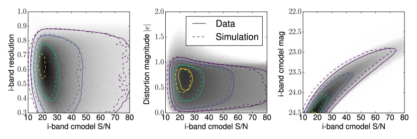
Finally, in Figure 9 we confirm that the shapes of the 2D joint distributions are well-matched between simulations and data, in addition to the shapes of the 1D distributions shown in previous figures.

5.2 Shape measurement uncertainty

Following the procedure from Section 4.3, we determined the per-component shape measurement uncertainty as a function of S/N and $R_{2}$. This function is shown in Figure 10, where the top panel shows the estimated value and the bottom panel shows the ratio of the values initially estimated by the HSC pipeline to those estimated from the simulations. The HSC pipeline values underestimate the measurement error in the distortion for all galaxies, with a typical 30 per cent underestimation but with some dependence on object properties.

Figure 10: The top panel shows the estimated per-component RMS distortion, $\sigma_{e}$, from the simulations as a function of the $i$-band cmodel S/N (horizontal axis) and the $i$-band resolution factor (vertical axis). The bottom panel shows the ratio of the catalog values of $\sigma_{e}$ to those estimated from the simulations, illustrating the fact that the catalog estimates are consistently too low compared to reality.

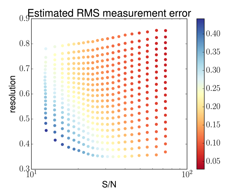
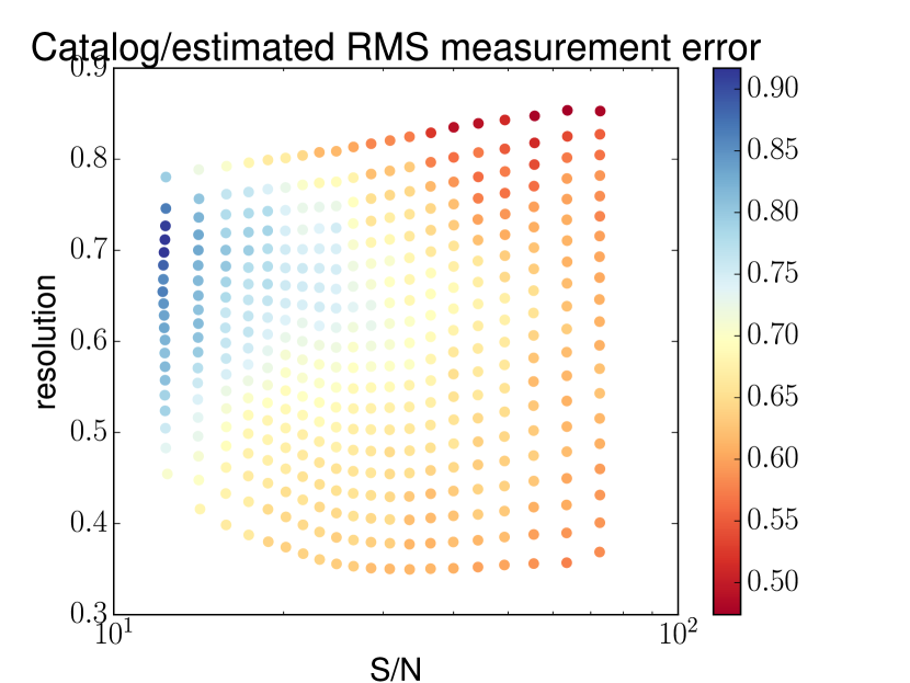
In order to estimate $\sigma_{e}$ for each galaxy in our catalog, we need a method of interpolating in this 2D plane. Given the steep dependences of $\sigma_{e}$ on these properties, we do not directly interpolate the function shown in Fig. 10. Instead, we fit for a power-law $\sigma_{e}(\text{S/N},R_{2})$ relation:

$$\sigma_{e}=0.264\left(\frac{S/N}{20}\right)^{-0.891}\left(\frac{R_{2}}{0.5}\right)^{-1.015}.$$ (18)

Then, we linearly interpolate the ratio of the estimated $\sigma_{e}(\text{S/N},R_{2})$ to that power-law based on the $\log_{10}{(\text{S/N})}$ and $R_{2}$ values, and use it to correct the power-law model. This means we are interpolating a function that is much closer to constant, varying by at most 25 per cent (and for typical parameter values, 10 per cent). For S/N and $R_{2}$ values outside the bounds of our sliding window, we simply use the nearest point within our sliding window for the interpolation of this ratio, but we still use the exact value of the power-law for the baseline $\sigma_{e}(\text{S/N},R_{2})$ model.

5.3 Implications for the RMS distortion

Following the process described in Section 4.4, we use the measurement noise function estimated in Section 5.2 to estimate the intrinsic shape dispersion in the real HSC shear catalogue. In other words, we use the real data, estimate the observed shape dispersion per component, and subtract off (in quadrature) the contribution from measurement noise based on the simulation-calibrated $\sigma_{e}$ values. The resulting intrinsic shape dispersion is shown in Figure 11. It is possible that the rise in the estimated dispersion at large $R_{2}$ is because that part of parameter space has a relatively higher fraction of unrecognized blends.

Figure 11: The per-component intrinsic shape dispersion estimated from the HSC shear catalog after subtracting the measurement error estimated from the simulations. For the majority of the galaxy sample (S/N$\lesssim 80$), the intrinsic shape dispersion is relatively flat as a function of object properties.

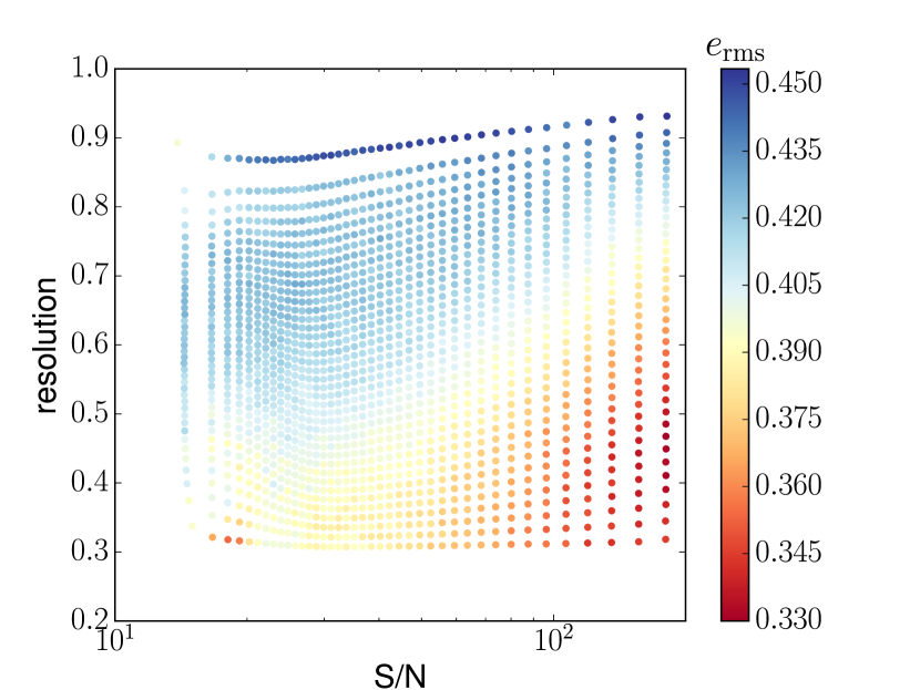
As shown, this function is relatively flat, with a value around 0.4 for most of parameter space. This corresponds to $\sigma_{\gamma}\approx\sigma_{e}/(2(1-0.4^{2}))\sim 0.24$. Each object in the catalog has a value of $e_{\text{rms}}$ linearly interpolated according to its value of resolution factor and log(S/N). Together with the $\sigma_{e}$ values from Section 5.2, these $e_{\text{rms}}$ uniquely determine the optimal (inverse variance) shape weighting given in Eq. (6).

Because of the way that we have estimated the intrinsic shape dispersion in the real data, by design it must be the case that $\sqrt{\langle\sigma_{e}^{2}+e_{\text{rms}}^{2}\rangle}=\sqrt{\langle 0.5(e_{1}^{2}+e_{2}^{2})\rangle}$ in bins of S/N and resolution factor in the real data. This is definitionally the case; however, a non-trivial test for whether we are missing dependencies on other parameters that should have been in our model is to test whether that equality holds when splitting the sample by other parameters. The reason this test is valuable is that in real data, we may split the sample by some other parameters, and we need to be able to use the model for $e_{\text{rms}}$ in order to infer the correct shear responsivity and hence the ensemble shear.

When using i-band magnitude as an additional parameter, we find that this equality holds to within 1 per cent for the entire magnitude range of our sample. Since the shear responsivity is roughly $1-e_{\text{rms}}^{2}$, this implies that uncertainties in the shear responsivity (and calibration) when dividing the sources by magnitude are at most 0.4 per cent. A more substantial concern arises when dividing the sample based on photometric redshift, which is a very common use case for tomographic weak lensing analyses. There, deviations from equality that are of order 8 per cent were seen for photometric redshifts between 1–1.5 and $\text{S/N}>40$, resulting in potential shear calibration biases of order 3 per cent at most (assuming that the entirety of this 8 per cent deviation is due to misestimation of $e_{\text{rms}}$ and not $\sigma_{e}$). Using our canonical parent sample of galaxies (sample 4) we cannot directly disentangle the possible misestimates of $e_{\text{rms}}$ and $\sigma_{e}$ in this redshift range, because we center our cutouts at the locations of HSC detections down to the detection limit without good redshift estimates. Hence we revisit parent sample 2 to understand this effect further. For that parent sample, we have high-quality 30-band photometric redshifts from COSMOS that can be used to reliably divide the sample based on redshift. Using those redshifts, we directly confirm that at fixed S/N and resolution factor, $\sigma_{e}$ has almost no dependence on redshift, while $e_{\text{rms}}$ depends on the joint distribution of redshift and S/N in a pattern consistent with what was seen in the real HSC data. The effect is such that for a sample in the photo-$z$ range $[1,1.5]$, there is a positive shear calibration bias of $+3$ per cent. Studies that divide the shear catalogue in ways that emphasize this redshift range, and that have a high level of statistical precision (such that a 3 per cent bias would be significant), should correct for this effect when modeling the shear signals.

5.4 Multiplicative shear calibration

To determine the baseline shear calibration in the absence of selection biases, we carry out the shear estimation process and calibration bias determination based on the process in Section 4.5 while using shape noise cancellation. Here, we always keep both objects in any 90^∘ rotated pair, imposing our weak lensing selection criteria on only one randomly chosen object in the pair and requiring them to both use the weight factor for that galaxy. By doing so, we ensure that our selection does not lead to some preference for the shear or PSF direction, enabling us to separate out basic features of the PSF-correction method such as model bias and noise bias from selection biases.

In Figure 12, we show the calibration bias as a function of S/N and resolution factor for the simulations overall, after subtracting off an unspecified constant value in order to preserve the blinding of our shear analysis. For reference, the bottom panel shows the statistical error for each of the points in parameter space on the top panel. Similarly to what was done for shape measurement error in Section 5.2, we fit $m(\text{S/N},R_{2})$ to a power-law in both parameters plus a constant additive offset, and interpolate a correction to that power-law based on the difference between the values in Fig. 12 to the best-fitting model. This defines our baseline calibration bias correction, which will be distributed with the public shear catalog.

Figure 12: Top: The component-averaged multiplicative shear bias $m$ in the 2D S/N vs. resolution factor ($R_{2}$) plane, with an unspecified offset to preserve the blinding of the shear calibration. Bottom: The statistical uncertainty in the per-bin $m$ estimates.

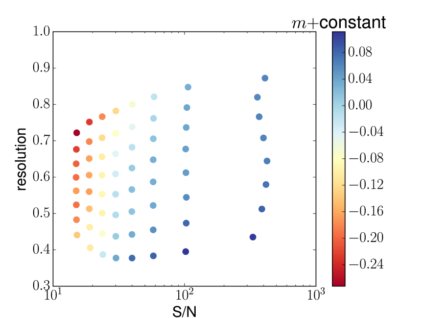
For this baseline correction, the calibration bias is more negative at low S/N and high $R_{2}$. The power-law scaling with S/N is $m\propto(\text{S/N})^{-1.24}$. The expected scaling with S/N for a pure noise bias in the case of Gaussian galaxies and PSFs and moments-based shape measurement would be $m\propto(\text{S/N})^{-2}$ (Hirata et al., 2004; Refregier et al., 2012), steeper than our results. However, it is not clear that the Gaussian approximation should be valid in this case given the realistic complexity in galaxy morphologies and PSFs, nor is the cmodel S/N estimate necessarily the one determining this relation.

The goal of the remainder of this section is to determine the validity and robustness of that calibration bias correction, and assign a systematic uncertainty to it. For example, we will explore the validity of the assumption that we can correct for calibration bias as function of just those two parameters, not including the magnitude or observing conditions explicitly. Since different lensing analyses will have different photometic redshift cuts (which correspond to complex cuts in the multidimensional color-magnitude space) and different area cuts (e.g., if using a galaxy cluster sample in a subset of the HSC survey region as lenses), this sensitivity analysis is necessary to define the systematic error budget due to shape measurement errors in the case of perfect PSF modeling.

In Mandelbaum et al. (2018) equation (6), a requirement on the systematic uncertainty in the shear calibration bias is given: $|\delta m|$ is required to be below 0.017 in order to avoid contaminating a cosmological galaxy-galaxy lensing analysis at the $0.5\sigma$ level, integrated over all scales. This is more stringent than the requirement derived for cosmic shear analysis, and hence we adopt this more stringent requirement. It is important to bear in mind two points about this number. First, calibration biases that are well-understood do not contribute here. If the biases are well-understood, we quantify and remove them using the aforementioned baseline correction. Second, the requirement is defined such that in a cosmological weak lensing analysis with the highest possible S/N for first year data would have systematic uncertainties due to shear calibration bias that can be effectively ignored in the analysis. Weak lensing analyses that achieve lower integrated S/N, for example due to use of a different lens sample or range of physical separations, can tolerate higher systematic errors than this requirement. Moreover, even the highest-precision measurements can still be done if the systematic errors exceed this requirement, but in that case, the failure to meet this requirement would require explicit tracking of the calibration bias uncertainty in the error budget, and the systematic uncertainty would no longer be negligible compared to the statistical error.

To carry out the sensitivity analysis and ascertain whether we achieve our requirements on shear estimation-related calibration bias, we proceed as follows:

• Define specially-selected subsamples of the shear catalog, e.g., with magnitude cuts, cuts on seeing, or other subsamples that do not correspond explicitly to selection in S/N and $R_{2}$.

• Estimate the shear in the simulations for those subsamples, including the calibration bias corrections as per the shear estimator in Eq. (9).

• Use the systematics model in Eq. (10) to estimate the residual calibration bias for the subsample.

By definition, this ‘round-trip’ exercise should give $m=a=0$ when using the entire weak lensing sample in the simulations, but may not give a calibration bias consistent with zero if our assumption that calibration bias depends only on S/N and $R_{2}$ is faulty. The results of this analysis are summarized in Table 2.

First, as shown in the table, our calibration bias corrections lead to an overall ensemble shear bias of $-0.001\pm 0.003$. This is what is expected by default.

The next section of the table shows the results when splitting in quartiles based on the PSF FWHM. This is meant to be an extreme case of what might happen when splitting up the survey based on region; in general, area-related cuts do not lead to as extreme differences in seeing as a strict seeing cut. As shown, when dividing into quartiles in the seeing, the resulting calibration biases exceed our requirements tolerances in two of the four cases. The implications of this finding are that weak lensing analyses that come with strict area cuts should evaluate the seeing distribution after their cuts, and then use the simulations to evaluate whether there are additional shear calibration biases that need to be removed for that special area definition. The results of this test are not relevant to the CMASS galaxy-galaxy lensing analysis that was used to set requirements, because the CMASS sample covers the entire HSC survey area.

The third section of the table shows what happens if we change the limiting magnitude from 24.5 to something lower (brighter). Since the calibration bias corrections were defined in terms of S/N instead of magnitude, any residual scalings with magnitude could result in a nonzero calibration bias for the ensemble. As shown, a cut at $i=24$, which eliminates tens of per cent of the sample, does not lead to any statistically significant calibration bias ($0.002\pm 0.002$). A cut at $i=23.5$, which is a very severe limiting of the sample, gives a marginal ($2.5\sigma$) detection of a calibration bias, $-0.005\pm 0.002$. Nonetheless, this uncertainty is still well within our requirement of $|\delta m|<0.017$, so this test does not raise any red flags for shear calibration uncertainties in cosmological weak lensing analyses.

Table 2: Sensitivity analysis for calibration bias correction $m$. We present the ensemble average $m$ for subsamples of the simulated galaxy sample defined below, after imposing our baseline calibration corrections.

Subsample definition	$m$
Sample overall	$-0.001\pm 0.003$
PSF FWHM: 1st quartile	$0.043\pm 0.005$
PSF FWHM: 2nd quartile	$0.004\pm 0.005$
PSF FWHM: 3rd quartile	$-0.019\pm 0.005$
PSF FWHM: 4th quartile	$-0.011\pm 0.005$
$i$ mag $<24$	$0.002\pm 0.002$
$i$ mag $<23.5$	$-0.005\pm 0.002$

Another potential contributor to systematic uncertainty in the shear calibration is failure of basic assumptions about the parent sample in the simulation. Since additional simulation sets are required to explore this source of uncertainty, we defer this investigation to Section 5.7. As mentioned earlier in this section, we explicitly separate out selection bias, and present estimates of its value and contribution to systematic error budget in Section 5.6.

The final contributor to systematic uncertainty in the shear calibration that we consider here is the incorrect assumption in the simulations that the noise correlation function is spatially invariant across the HSC survey (see Section 3.2). Our calculations described there indicate that the typical spatial scale on which the noise correlations varies is larger than the typical size of galaxies. Hence, the primary impact of our simplified assumption is that a given galaxy that would be seen in the HSC survey with several different levels of noise correlation (if observed at different places on the sky) actually is simulated with only a single value of noise correlation. As shown by Gurvich & Mandelbaum (2016), a given realization of that galaxy $j$ would have a different effective S/N_j when changing the level of noise correlations even for fixed PSF and noise variance, and hence different levels of shear calibration bias (driven by noise bias) $m_{j}$ for the different realizations. If $\langle m_{j}\rangle$ across those realizations is not equal to the estimated calibration bias $m$ at the single simulated level of noise correlations, this would mean that our shear calibration bias estimates are incorrect.

Using multiple noise realizations of individual galaxy models, we have estimated how (for typical galaxies) the effective S/N changes when the PSF and noise variance are fixed, but the level of noise correlations varies within the level seen in individual patches in HSC. We find that within that narrow range of variation, the S/N is linearly proportional to the level of noise correlations at a separation of one pixel, and the range of S/N variation implied is $\pm 2$ per cent from the S/N at the average level of noise correlations across the patch. Since we have found that $m\propto(\text{S/N})^{-1.24}$, this implies that the value of $m$ is changing by $\pm 2.5$ per cent of its value. In other words, for a point in parameter space where we have estimated $m=-0.1$, the variation in noise correlations across the survey means it really ranges from $[-0.1025,-0.976]$, which is far below both the statistical uncertainty in $m$ and other sources of systematic uncertainty in $m$.

5.5 Additive biases

In this section we show our results for the additive biases following the same methodology as for multiplicative biases in Section 5.4.

In Figure 13, we show the additive bias as a function of S/N and resolution factor for the simulations overall. For reference, the bottom panel shows the statistical error for each of the points in parameter space on the top panel. Similarly to what was done for shape measurement error in Section 5.2, we fit $a(\text{S/N},R_{2})$ to a parametric model

$$a\propto(R_{2}-R_{2,0})\left(\frac{\text{S/N}}{20}\right)^{Q},$$ (19)

with the constant of proportionality, $R_{2,0}$, and $Q$ being free parameters. Then we interpolate a correction to that power-law based on the difference between the values in Fig. 13 to the best-fitting model. This defines our baseline additive bias correction in the catalog.

Figure 13: Top: The component-averaged additive shear bias $a$ in the 2D S/N vs. resolution factor ($R_{2}$) plane. Bottom: The statistical uncertainty in the per-bin $a$ estimates.

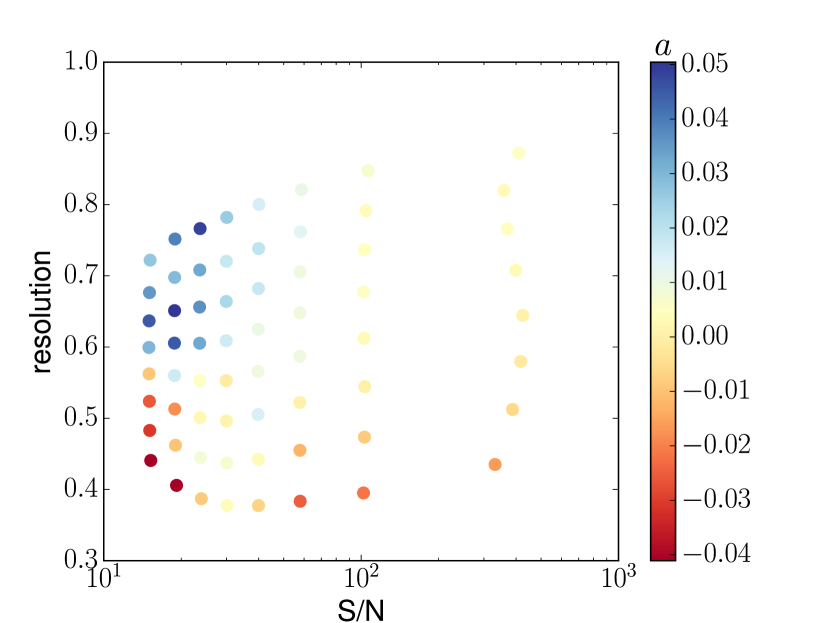
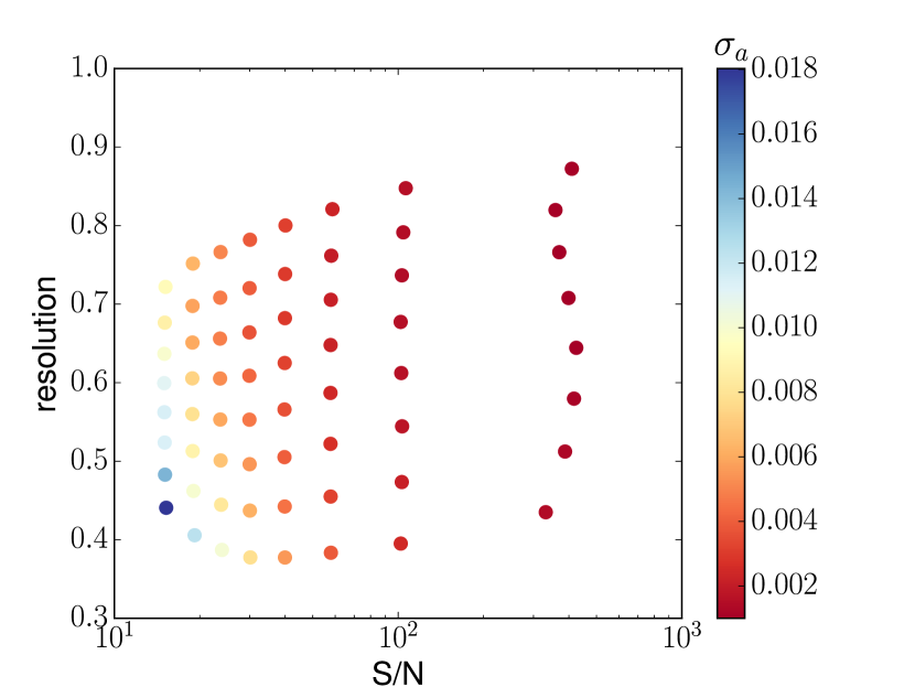
For this baseline correction, the additive bias is negative at low $R_{2}$ and positive at high $R_{2}$, with the deviations from zero being significant only for $\text{S/N}<60$ or $R_{2}<0.4$. When fitting the model in Eq. 19, the power-law scaling with S/N is $a\propto(\text{S/N})^{-1.07}$, and the cross-over value $R_{2,0}=0.51$.

Similarly to what was done in the previous subsection with the multiplicative calibration bias, we check the sensitivity of this $a$ estimate to how the sample is defined. The results of this analysis are summarized in Table 3.

Table 3: Sensitivity analysis for additive bias correction $a$. We present the ensemble average $a$ for subsamples of the simulated galaxy sample defined below, after imposing our baseline calibration corrections.

Subsample definition	$a$	$\delta a^{2}$
Sample overall	$-0.008\pm 0.001$	$2\times 10^{-5}$
PSF FWHM: 1st quartile	$-0.004\pm 0.002$	$2\times 10^{-5}$
PSF FWHM: 2nd quartile	$0.001\pm 0.002$	$4\times 10^{-6}$
PSF FWHM: 3rd quartile	$-0.012\pm 0.003$	$7\times 10^{-5}$
PSF FWHM: 4th quartile	$-0.006\pm 0.003$	$3.6\times 10^{-5}$
$i$ mag $<24$	$-0.010\pm 0.001$	$2\times 10^{-5}$
$i$ mag $<23.5$	$-0.007\pm 0.001$	$1.4\times 10^{-5}$

In Mandelbaum et al. (2018) below equation (24), a requirement on the systematic uncertainty in the value of $a^{2}$ is given: $\delta(a^{2})$ is required to be below $8\times 10^{-4}$ in order to avoid contaminating a cosmic shear analysis in a way that noticably inflates the systematic error budget. Given the statistical error in the simulations, as shown in Table 3, for our baseline model we can determine $a$ well enough that the statistical error $\delta a^{2}$ is more than an order of magnitude below our requirements. As a consequence, the systematic uncertainties are more important.

Comparing the four quartiles in PSF FWHM, we see that the variation in $a^{2}$ from the two most extreme values is $1.4\times 10^{-4}$, well below our already-conservative requirements. For this reason, we need not worry when dividing up the sample in ways that result in different seeing distributions that the additive bias behavior will vary significantly from our baseline model. Similarly, the cuts on magnitude induce variations in $a^{2}$ that are also below our requirements. We conclude that additive biases due to PSF correction methods can be well-controlled below the level needed with the existing simulations, without significant ambiguity when imposing other cuts on the galaxy sample. Other sources of additive bias, such as PSF modeling errors (as quantified in Mandelbaum et al. 2018), are likely to be more important.

5.6 Selection bias

Below we separately describe the results of our analysis of the two types of selection bias described in Section 4.6.

5.6.1 Selection bias due to weights

We directly compared the simulation analysis with shape noise cancellation without enforcing the same per-object weight for each galaxy in a pair, versus the results when we did enforce sameness of weights. The resulting multiplicative and additive selection biases are called $m_{\text{wt}}$ and $a_{\text{wt}}$. We found that $a_{\text{wt}}$ was consistent with zero within the noise, but there was a highly statistically significant $m_{\text{wt}}$ that depends on galaxy properties; see Figure 14. As shown, this bias is negative and reaches a maximum magnitude of $-0.045$ at high S/N and $R_{2}$, while it is positive and reaches a maximum magnitude of $0.055$ at low S/N and $R_{2}$.

Figure 14: The component-averaged shear calibration bias $m_{\text{wt}}$ due to weight bias in the 2D S/N vs. resolution factor ($R_{2}$) plane.

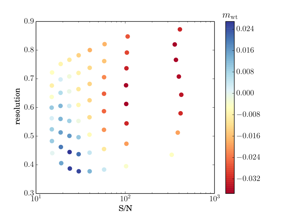
We have used the $90^{\circ}$ rotated pairs to confirm that the sign of the constant of proportionality in Eq. (11) when $X$ is the lensing weight is consistent with Fig. 14. That is, at low S/N and $R_{2}$, the lensing weight is larger for galaxies aligned with the shear than for those oriented perpendicular to it, while at high S/N and $R_{2}$, it is smaller for galaxies aligned with the shear.

Since this weight bias depends on the location in this 2D parameter space, we have used the same process as in Sec. 5.4 to estimate and remove its effects. The $m$ values given in the catalog include the baseline multiplicative calibration biases due to model and noise bias, along with $m_{\text{wt}}$.

The process described in this section implicitly assumes an analysis of a subset of the data with a representative PSF FWHM distribution. Carrying out a sensitivity analysis for any residual biases due to $m_{\text{wt}}$ varying with the PSF size leads to a conclusion that there are mild residuals, of order 0.5 per cent averaged across the whole source sample, when considering extreme quartiles in PSF size. Since we have already concluded in Section 5.4 that the baseline calibration bias values $m$ (due to noise and model bias) have an even more significant variation for the extreme quartiles in PSF size, and advocated for caution in analyses with highly non-representative PSF FWHM distributions, that recommendation will also apply to the $m_{\text{wt}}$ variation with seeing.

5.6.2 Selection bias due to cuts

As described in Section 4.6, our formalism involves estimating the multiplicative and additive selection biases by comparing shear estimation for the sample overall without vs. with $90^{\circ}$ rotated pairs, using that to define the constants of proportionality in Equations 16 and 17, and checking for consistency as we modify the values of the cuts in resolution factor and magnitude.

For resolution factor, we estimate the shear (including corrections for other forms of shear calibration bias) with a fixed value for the lower limit in resolution factor, $R_{2}=0.3$, as we stop requiring shape noise cancellation around that boundary. We can check that the formalism described previously is consistent with the results as we vary $p(R_{2}=0.3)$ (i.e., $p(\hat{X})_{\text{edge}}$) by cutting the sample in other ways and directly inferring the selection bias $m_{\text{sel}}$. The motivation for framing the test in this way – with a fixed lower limit in resolution factor – is that there is no compelling scientific reason to vary the lower limit from $R_{2}=0.3$. However, as we impose cuts on photometric redshifts, the distribution of $R_{2}$ values gets mildly shifted such that the relative fraction near the edge of the sample changes at the level of tens of per cent (see section 8 of Mandelbaum et al., 2018, for details of how photometric redshift cuts modify other sample properties). Thus the most important thing is to confirm that the proportionality between $m_{\text{sel}}$ and $p(R_{2}=0.3)$ in Eq. (16) holds, and determine the constant of proportionality.

Rather than varying photo-$z$ cuts and checking this relationship with the simulations, we consider more extreme variations in $p(R_{2}=0.3)$ as a more stringent test of our formalism. To do so, we impose strict upper limits in $R_{2}$ to remove large portions of the sample, but do so while imposing shape noise cancellation at that upper edge. For example, if we impose an upper limit at the median $R_{2}$ value, then $p(R_{2}=0.3)$ should double, and hence the selection bias should as well. Our results are summarized in Fig. 15. As shown, the ratio $m_{\text{sel}}/p(R_{2}=0.3)$ is indeed consistent with constant even given a factor of three variation in $p(R_{2}=0.3)$, validating our adopted formalism. For the entire shape sample, the resulting multiplicative bias is $0.010\pm 0.003$; more generally, if $m_{\text{sel}}=A\,p(R_{2}=0.3)$ then $A=0.0087\pm 0.0026$. While low-S/N weak lensing measurements such as cluster lensing with individual clusters can afford to ignore a percent-level bias, more precise galaxy-galaxy or cluster-galaxy lensing measurements, or cosmic shear measurements, should use this equation and the actual weighted $p(R_{2})$ for their sample with all photometric redshift or other cuts to correct for the impact of selection bias due to our lower limit in $R_{2}$.

Figure 15: This plot shows the empirically-determined (in the simulations) ratio of the multiplicative selection bias due to our lower limit in $R_{2}$ (resolution factor) to the value of $p(R_{2})$ evaluated at that lower limit, which should be a constant according to our formalism. The horizontal axis shows the imposed upper limit in $R_{2}$ that was used to induce variation in $p(R_{2}=0.3)$ while maintaining shape noise cancellation and hence not causing additional selection bias. The color bar shows the actual value of $p(R_{2}=0.3)$ for each point. Errorbars are correlated between the points due to the use of at least a fraction of the same simulated source galaxies.

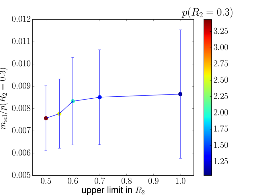
Using this same approach, we find no statistically significant evidence for additive selection biases due to either our resolution factor or magnitude cuts, or multiplicative selection biases due to magnitude cuts. The errorbars are similar to those for the resolution factor estimate of selection bias, $\pm 0.003$. We therefore only impose a correction for multiplicative selection bias due to the resolution factor cut.

5.7 Dependence of results on parent sample in simulations

As described in Section 3.3, there are several significant factors in selection of the parent sample for the simulations. In this subsection, we present selected results from simulations produced using parent samples 1–3, in order to ascertain the sensitivity of our results to parent sample selection, and learn about the systematic uncertainty in our results.

Referring back to Table 1, we hope to learn the following things by making certain well-defined comparisons:

• Comparing the shear calibration biases for simulations with parent samples 1 and 2 will reveal the importance of realistic galaxy morphology as compared to simple parametric models.

• Comparing results for parent samples 1 and 3 will (at least partially) reveal the impact of nearby objects on the outskirts of the primary objects we are measuring. The reason we are able to learn this is that the primary differences between these samples is that in sample 3 we carry out deblending only in HSC, without any a priori deblending in COSMOS (unlike for sample 1).

• Comparing results for parent samples 3 and 4 will reveal the impact of selecting galaxies in HST based on the cuts given in Section 3.3, rather than selecting them based on HSC imaging.

Figure 16 shows differences in calibration bias $m$ and additive bias $a$ as a function of S/N (left) and resolution factor (right), for these three pairs of simulation sets. It is important to bear in mind that when making this comparison in a single dimension (S/N or $R_{2}$), we are effectively marginalizing over the distribution of other galaxy properties. For example, at a given S/N value, one could in principle get different $m$ values even if the curve of $m(\text{S/N},R_{2})$ is the same for two simulation sets, but the distribution of $R_{2}$ values ($\mathrm{d}N/\mathrm{d}R_{2}$) at that S/N differs for the two simulation sets. Hence these plots implicitly include information not just about $m$ and $a$ as a function of object properties, but also about the joint distribution of object properties.

Figure 16: Differences in multiplicative bias $\Delta m$ (top) and additive bias $\Delta a$ (bottom) as a function of the galaxy S/N (left) and resolution factor (right) when comparing pairs of simulations with the different parent samples described in the text. This figure illustrates the importance of the postage stamp creation process in determining the shear calibration.

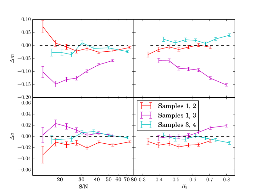
5.7.1 Impact of realistic galaxy morphology

To consider the impact of realistic galaxy morphology vs. parametric models, we consider the curves for $\Delta m$ and $\Delta a$ on Figure 16 labeled ‘Samples 1, 2’. As shown, the $\Delta m$ curve in the top left panel of Figure 16 goes from $\sim 0.07\pm 0.02$ at S/N$\sim$15 to $\sim-0.02\pm 0.005$ at S/N$\sim$80. The crossing point at S/N$\sim$20 corresponds to the point at which our distribution of S/N values is cutting off (see Fig. 8). As a result, the average $\Delta m$ integrated over the whole sample is $-0.014\pm 0.003$. This is consistent with the results for many shear estimation methods in the GREAT3 challenge, where parametric models vs. realistic galaxy morphology resulted in differences in shear calibration of $\lesssim 1$ per cent (Mandelbaum et al., 2015). Hence realistic morphology is subdominant to effects like noise bias (which results in variations in shear calibration that are an order of magnitude larger, as shown in Fig. 12).

The bottom left panel of that figure suggests that realistic galaxy morphology can result in differences in $a$ that are of order 0.01–0.02, consistently across all S/N values. The sign of this effect is such that the additive bias is consistent with zero for parametric models, but nonzero for realistic galaxy morphology. This suggests that it is harder for re-Gaussianization to remove the PSF anisotropy from the galaxy shapes when the galaxy models deviate more strongly from simple elliptical models, and hence is a signature of model bias.

5.7.2 Impact of nearby objects

To consider the impact of nearby objects in the COSMOS images, we consider the curves for $\Delta m$ and $\Delta a$ on Figure 16 labeled ‘Samples 1, 3’. As summarized in Table 1, the key difference between these samples is that for sample 1, we used postage stamps that were masked based on using the Sextractor deblender to identify nearby objects in COSMOS and mask them out with correlated noise. In contrast, for sample 3, the nearby objects were not masked, and we ran the HSC object selection and deblending routines. We know that if structure is near enough to the central galaxies we are analyzing, then it can be easily deblended in COSMOS but cannot possibly be recognized as distinct structures in any ground-based imaging, even with the excellent typical seeing in the HSC $i$-band Wide layer images (median PSF FWHM of 0.58″ for the shear catalog, Mandelbaum et al. 2018). Sample 3 simulations will include both recognized and unrecognized blends, while sample 1 will not.

Clearly $\Delta m$ for these two cases is very large, ranging from $-0.1$ (more negative bias for sample 3) at S/N$\sim$20 to $-0.03$ at S/N$\sim 80$. Alternatively, considering the variation with resolution factor, the difference ranges from -0.07 near our resolution factor limit $R_{2}\sim 0.3$, to -0.15 at $R_{2}\sim 1$. We note that the galaxies contributing to the two curves at a given S/N value are not necessarily the same in the two simulation sets, so this can be a combination of multiple effects: biases at fixed S/N and different biases for objects that have been scattered coherently across S/N bins. Whatever the origin of the effect, it is clearly the most striking finding to come from comparing simulations with different parent samples. Since this difference is many times our requirement on systematic uncertainty in $m$ of 0.017, we need to definitively understand the origin of this difference and ascertain which sample more accurately reflects reality.

A hint at the resolution of this problem comes from Figure 17, which shows the distribution of the $i$-band magnitudes (top) and resolution factors (bottom) for galaxies passing the weak lensing cuts in the data and in all four parent samples. The data and parent sample 4 curves on this plot are the same as those that were shown in Fig. 8. As shown, the simulations generated using parent samples 1 and 2 (which is similar to sample 1 in that the masking of nearby objects was also carried out) have distributions of magnitude and resolution factor that are strikingly different from those in both real data and in the simulations generated using parent samples 3 and 4 (neither of which has nearby objects masked out in the original COSMOS images).

Figure 17: Normalized distribution of $i$-band magnitude (top) and resolution factor $R_{2}$ (bottom) for all galaxies passing the lensing cuts in the data and the simulations with the four different parent samples, as shown in the legend. Once we use our procedure defined in this work to define the galaxy postage stamps without masking of nearby galaxies (samples 3 and 4), the simulated galaxy properties agree well with those in the data.

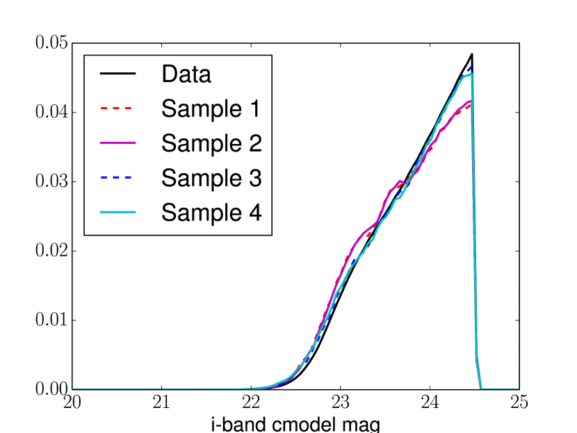
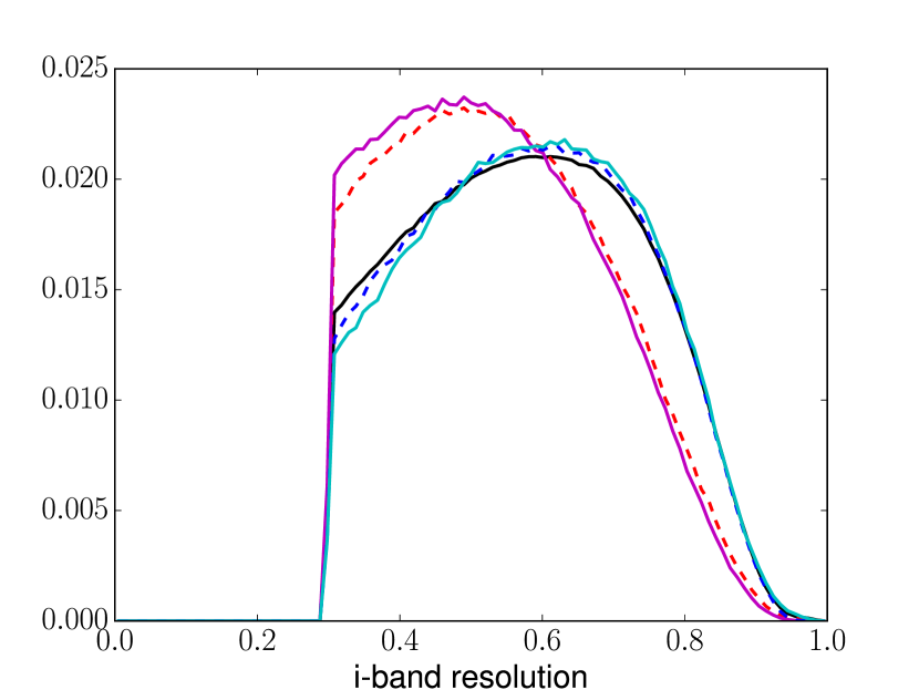
The histograms in Figure 17 appear to be telling us that the galaxies in the simulations made with parent sample 1 are typically brighter and smaller than those in real data. Since parent samples 3 and 4 have nearby objects in COSMOS that are not masked, it seems clear why we might measure galaxies as being typically larger in simulations made with those parent samples compared to parent samples 1 and 2: the extra light on the outskirts of galaxies may inflate the measured galaxy sizes and resolution factors. Hence the differences in resolution factor are physically understandable, and the fact that samples 3 and 4 match the data so much better than samples 1 and 2 in this regard strongly suggests that the simulations with samples 3 and 4 have captured a physical effect that is important in determining the apparent resolution factor distribution in real data, due to either the inability to distinguish blend systems that can be recognized in HST data or biased resolution factors for recognized blend systems. As for the difference in magnitude distribution, since these are normalized histograms, they must integrate to the same value. However, on average, inclusion of light from nearby objects into the central object light profile is going to make objects appear brighter in the simulations made with parent samples 3 and 4, scattering them into the sample, whereas with samples 1 and 2 they would have failed our weak lensing cuts. This explains why parent samples 3 and 4 have relatively more objects that are near our adopted faint magnitude limit.

The above arguments are valid for two possible explanations of what is going on: (1) as hypothesized above, light from nearby objects that cannot possibly be deblended in HSC images is artificially inflating the sizes and magnitudes of some objects, or (2) that the masking process artificially shredded some low surface-brightness galaxies in the COSMOS images in parent samples 1 and 2, and thus the masking process was altogether incorrect. Visual inspection suggests that for objects brighter than 24th magnitude, process (1) dominates, while near the limiting magnitude, it is different to discriminate between these two options, and likely both are occurring at some level. However, regardless of the explanation, Figure 17 tells us that if we want the simulations to accurately represent all relevant image processing effects in the data, we need to use parent samples 3 and 4, and carry out full object detection and deblending.

While we have shown that the galaxies in the simulations made with parent sample 3 are systematically larger than those made with parent sample 1, those distributions do not fully explain the large difference in shear calibration seen in the two simulation sets. To do so, we need to show that for the same galaxies, the resolution factor is larger in simulations made with parent sample 3 rather than sample 1 (i.e., that the difference in $R_{2}$ distributions cannot be fully explained by new objects scattering in across the boundary of our cuts). Since we used the same sample of objects from COSMOS, simply swapping in unmasked postage stamps for the masked ones with the same simulated PSFs, it is trivial to identify objects in the two sets of simulations that came from the same object in COSMOS. However, we can do better than that: by comparing the masked and unmasked postage stamps, it should be possible to define a statistic quantifying how much fractional contamination of the object light profile we expect in the HSC simulations. Conceptually, our test statistic $f_{\text{contam}}$ is defined as the ratio of two quantities: the weighted sum of flux in pixels that are masked out for sample 1, divided by the weighted sum of flux in all pixels in the unmasked postage stamps. The weight function is defined by convolving the original COSMOS light profile by a Kolmogorov approximation to the simulated HSC PSF, since we are trying to quantify how much the nearby light would affect the light profile as seen in HSC. If our explanation is correct, then the difference in resolution factor and/or magnitude $\Delta R_{2}$ and $\Delta$mag between the simulation sets should be a strong function of $f_{\text{contam}}$, nearing zero for apparently isolated objects.

To identify a statistical correlation between $f_{\text{contam}}$ and $\Delta R_{2}$ and/or $\Delta$mag, we do not calculate a correlation coefficient, because we do not necessarily expect a linear relationship. Instead, we divide the sample based on an $f_{\text{contam}}$ value corresponding to low (few per cent) contamination of the light profile vs. higher contamination, and compare the typical $\Delta R_{2}$ and $\Delta$mag values for objects above and below that level of contamination. This dividing line happens to fall around the 70th percentile in $f_{\text{contam}}$. We find that if we split the sample into those above vs. below the 70th percentile in $f_{\text{contam}}$, the $\Delta R_{2}$ is typically 0.07 vs. 0.01. That bias in resolution factor should give rise to a difference in shear calibration that is of order 0.06 (with the exact value depending on the entire distribution of object properties). It is therefore plausible that between this bias in $R_{2}$ and the fact that new objects are scattered into the sample by the light from nearby objects, changing the galaxy population overall, the shear calibration bias differences seen in simulations with samples 1 and 3 can be entirely explained. Similar, $\Delta$mag for those above vs. below the 70th percentile in our test statistic is $-0.15$ vs. $-0.02$, supporting our argument that some galaxies from below the flux limit in the simulations with parent sample 1 are getting scattered across our cuts and into the weak lensing-selected sample in parent sample 3 (and the real data).

By splitting the galaxy population in the sample 3 simulations at the 70th percentile in our test statistic, we have also directly ascertained that the shear calibration biases for the two subpopulations within that simulation sets differ by approximately the amount expected based on this bias in the $R_{2}$ values.

This dramatic effect due to different parent sample populations is related to an effect that has been reported elsewhere in the literature. Hoekstra et al. (2015) carried out tests of shear estimation using the moments-based KSB method, and argued based on their figure 7 that in order to properly estimate the shear calibration for a sample with some limiting magnitude $m_{\text{lim}}$, it is necessary to include galaxies about 1.5 magnitudes fainter than $m_{\text{lim}}$ in the simulations. Their explanation was that these galaxies contribute a small amount of light that essentially looks like correlated noise clumps on the outskirts of the galaxies brighter than $m_{\text{lim}}$. It is worth considering that both KSB and re-Gaussianization are moments-based methods that use weighted moments to correct the observed shapes for the blurring by the PSF. If the nearby objects systematically cause a positive bias in the observed size of the galaxies, then the estimated shears will systematically be too low by a similar factor for both methods. It is less obvious whether this effect will cause a similar problem for model-fitting methods, and likely depends on implementation details of the method. However, there is an important difference between what was reported in Hoekstra et al. (2015) and what is shown here. They report that the primary cause of the effect they see is due to unresolved backgrounds contributing correlated noise. In HSC, we have set a quite conservative magnitude limit, and the objects that are nearby and were masked in parent sample 1 would typically not be below the detection limit in HSC (despite the fact that, on their own, they would be too faint to pass our conservative weak lensing cuts). Thus we conclude that in HSC, the effect we are seeing is primarily due to light from nearby objects above the detection threshold that lead to the aforementioned bias in resolution factor and shear. Indeed, unresolved backgrounds contribute correlated noise near our simulated galaxies in both simulation sets 1 and 3.

For the Dark Energy Survey Year 1 analysis, Samuroff et al. (2018) used simulations to study the impact of nearby objects on shear estimation, and identified a net calibration bias (from several effects combined) that is of order 30 to 100 per cent of the effect seen in this work, depending on the sample selection. They find that removal of nearby objects is an effective mitigation scheme, while for HSC we do not expect this approach to be effective because our depth results in a higher fraction of unrecognized blends, despite the smaller seeing size. As noted in that work, it seems unlikely that this effect can be represented as purely a scale-independent calibration bias; however, for the level of precision in shear correlation functions in the first-year HSC analysis, this approximation is likely to be sufficient.

Returning to the trends in $\Delta m$ between simulations made with samples 1 and 3 in Figure 16, we found more severely negative calibration biases at low S/N and high $R_{2}$. This makes sense given the origin of the effect. Low S/N objects will have a higher fractional contamination of their light profile by nearby objects, resulting in a larger bias in $R_{2}$ and the shear. Similarly, objects with larger size may have been artificially inflated by this effect, or may be truly large objects with low surface brightness, in either case resulting in a larger shear bias.

In principle, the size of this shear bias should depend on the number density of sources of sufficient flux to cause a measurable bias in the shape of the galaxies of interest. Assuming only galaxies within a fixed $\Delta$mag of the limiting magnitude can have an effect, and knowing that the number density of brighter objects is lower than that of fainter objects, we expect a smaller effect for samples with a brighter limiting magnitude. Using the simulations, we can directly measure this trend by changing the limiting magnitude from 24.5 to something brighter than that, and comparing parent samples 1 and 3. The results for the average $\Delta m$ (over the entire samples brighter than some limiting mag) are shown in Fig. 18. The $\Delta a$ (not shown on the plot) is in all cases consistent with zero. As shown, the shape of the curve is largely what we expect; however, there is a slight turnover at the brightest limiting magnitude that is difficult to explain. Unfortunately we cannot test any further restriction on the sample, as the number of galaxies in the simulations brighter than $i=22$ is too small.

Figure 18: Additional calibration bias due to the presence of nearby objects in the galaxy postage stamps, as a function of the limiting magnitude of the sample selected for shear estimation.

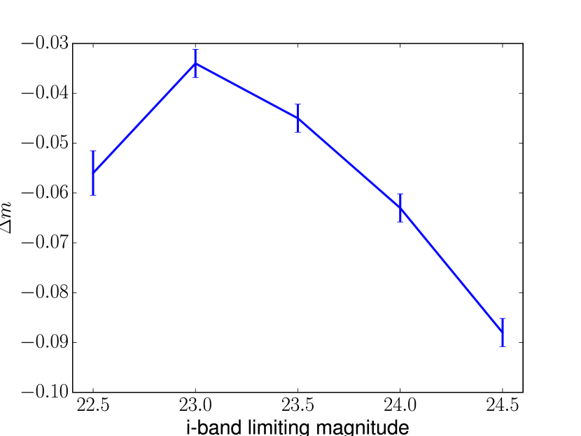
Finally, we note that another difference between samples 1 and 3 shown in Table 1 is the imposition of the ‘marginal’ selection criteria on the simulations made with sample 1. We have explicitly tested whether this can be responsible for some of the differences seen, by imposing the ‘marginal’ cut on the simulations with parent sample 3 after their creation, and found that the effect of this cut on the shear calibration in the simulations is negligible.

5.7.3 Impact of HSC vs. HST selection

To consider the impact of selecting the galaxies with the flag cuts described in Section 3.3.1 in HST, versus selecting them based on their detectability in HSC as described in Section 3.3.4, we consider the curves for $\Delta m$ and $\Delta a$ on Figure 16 labeled ‘Samples 3, 4’. As shown, the $\Delta m$ curves suggest that different choices of how to select the galaxies can induce $\sim 2$ per cent differences in shear calibration. However, as shown in Figure 17, the resulting differences in the selected object properties are quite small.

In this case, none of our diagnostics revealed obvious flaws with the sample 3 simulations. Nonetheless, as described in Section 3.3.1, diagnostics of the parent samples indicated that the ground-based selection flag applied to the COSMOS sample preferentially removes galaxies that are near other bright galaxies from the sample. Hence, as a matter of principle, we adopt sample 4 as the fiducial one.

6 Conclusions

The over-arching goal of this paper is to use simulations with a realistic galaxy population, and HSC imaging conditions, to constrain certain weak lensing shear systematics that are difficult to identify using the data itself, devise corrections for our best estimates of those systematics, and estimate systematic uncertainties in those corrections in order to build our systematic error budget for cosmological weak lensing analyses with the HSC weak lensing shear catalogue described in Mandelbaum et al. (2018). For this purpose, we have used large suites of simulations with galaxy images directly from the HST COSMOS imaging, selected based on deep coadded HSC imaging, with the HST PSF removed, lensing shear applied, and then applied further image manipulations to look like the HSC survey data. While the analysis used postage stamp images, no attempt was made to mask out nearby objects from the outset, and the selection and deblending parts of the HSC pipeline were run. Hence the impact of nearby objects and unrecognized blends (blends of two or more objects that are not recognized as such by the HSC pipeline) is implicitly included, albeit with the assumption that the two objects have the same shear.

More specifically, the tests in this paper were focused on understanding multiplicative and additive shear biases due to the following effects:

1. Model bias due to fully realistic galaxy morphology (no parametric models) and other fundamental failures of the assumptions of the re-Gaussianization shear estimation method;

2. noise bias;

3. the impact of light from nearby objects that are properly detected and deblended;

4. unrecognized blends that are at the same or similar redshifts;

5. selection bias due to the weight factors used for ensemble averages depending on the galaxy shape (‘weight bias’); and

6. selection bias due to the quantities used to place cuts on the sample depending on the galaxy shape.

This list is by no means an exhaustive coverage of the observational systematic error budget for a cosmological weak lensing analysis. There are three types of effects that were excluded. The first type of effects were excluded because it is not possible to quantify them with the type of single-band simulations made here: photometric redshift errors; the impact of unrecognized blends not at the same redshift (and not carrying the same shear) for both shear estimation and photometric redshifts; and selection biases in shear induced by photometric redshift cuts. The second type of effects were excluded because they are constrained elsewhere (Mandelbaum et al., 2018): PSF modeling errors, relative astrometric errors, and stellar contamination. There is a final class of effects that were not covered here because we anticipate they are too low-level to form a significant part of the HSC first-year weak lensing error budget: e.g., the impact of chromatic PSFs or non-weak shear.

In evaluating the quality of the simulations themselves, and the fidelity with which they represent the data, we identified an important issue with the input galaxy population. Based on our findings, the process of masking out nearby objects in the original HST images makes it impossible to simulate a realistic ground-based survey, because the non-negligible fraction of unrecognized blends that will not be accurately represented if nearby objects in HST images are masked. The simulated galaxy populations appear to be too small on average, and have the wrong magnitude distribution, if the masked images are used. This was found to be an important factor in shear estimation, which we have interpreted as a sensitivity of the re-Gaussianization algorithm to both light from nearby objects and unrecognized blends. Hence, the results that we use for science are the ones that include the impact of both recognized and unrecognized blends.

We have quantified and removed non-negligible systematic biases in the ensemble shear estimates due to the six sources of bias enumerated earlier in this section. In Sections 5.4 and 5.5, we have quoted requirements on the uncertainties in multiplicative and additive bias from Mandelbaum et al. (2018), and discussed how well we meet those requirements for the specific set of systematics addressed in this paper. We found that the additive biases were not strongly sensitive to divisions of the source sample based on seeing size or magnitude, and hence cuts on the source sample for a real analysis should not cause a failure to meet our requirements. The multiplicative bias corrections defined here were found to have a modest dependence on seeing size, such that if we use a special sample of lenses that only resides in a particular region of the survey that has anomalously good or bad seeing, it may be necessary to redefine the calibration factors using the simulations. However, our core cosmology analyses that use the entire first-year area set our most stringent requirements, and are not subject to this limitation. Similarly, cuts in magnitude (which was not one of the parameters used to define our calibration corrections) were found to cause marginally statistically significant ($2.5\sigma$) multiplicative biases, but these were still $3\times$ lower than the conservative requirements set in Mandelbaum et al. (2018), and hence we do not anticipate failures of our multiplicative bias corrections for magnitude- or color-selected samples.

Overall, our findings suggest that the quantifiable biases due to the causes investigated in this paper are significant in magnitude, but understood and therefore corrected at the level of precision required for first-year HSC weak lensing analysis (to within roughly 1 per cent). In terms of the future outlook, having an independently-developed shear estimation method with completely different assumptions will be an important sanity check on the results in this paper; forthcoming results from Armstrong et al. (in prep.) should provide this sanity check. In addition, one of the key results of this paper – the sensitivity of the results to the simulated galaxy population – suggests that for future shear catalogs in HSC covering larger areas and requiring better systematics control, we may wish to adopt shear calibration methods that do not require the ground-up generation of realistic image simulations, such as the metacalibration method (Huff & Mandelbaum, 2017; Sheldon & Huff, 2017). A further benefit of this change is that it would enable us to use galaxy samples fainter than $i=24.5$, which would otherwise require deeper HST training data.

Appendix A Shape measurement error formalism

This appendix outlines the formalism for using $90^{\circ}$ rotated pairs of galaxies in the simulations to estimate the shape measurement error as a function of galaxy properties. The formalism below assumes the shape definition in Equation (1).

For each such pair, after analyzing the simulations with the HSC pipeline, we have an estimate of the distortion for both galaxies, $\hat{e}$ and $\hat{e}_{\text{rot}}$ (consider these as two-component complex ellipticities). These are related to the true intrinsic shape $e_{\text{int}}$ (or $-e_{\text{int}}$ for the 90^∘ rotated version), the lensing reduced shear $g$, and the independent measurement errors for the two realizations $\delta e$ and $\delta e_{\text{rot}}$ as:

$$\hat{e} =\frac{e_{\text{int}}+2g+g^{2}e_{\text{int}}^{*}}{1+|g|^{2}+ge_{\text{int}}^{*}+g^{*}e_{\text{int}}}+\delta e$$ (20)

$$\hat{e}_{\text{rot}} =\frac{-e_{\text{int}}+2g-g^{2}e_{\text{int}}^{*}}{1+|g|^{2}-ge_{\text{int}}^{*}-g^{*}e_{\text{int}}}+\delta e_{\text{rot}}.$$ (21)

In the weak shear limit ($g^{2}\approx|g|^{2}\approx 0$), these equation simplify to

$$\hat{e} =\frac{e_{\text{int}}+2g}{1+ge_{\text{int}}^{*}+g^{*}e_{\text{int}}}+\delta e$$ (22)

$$\hat{e}_{\text{rot}} =\frac{-e_{\text{int}}+2g}{1-ge_{\text{int}}^{*}-g^{*}e_{\text{int}}}+\delta e_{\text{rot}}$$ (23)

or, even further, to

$$\hat{e} =(e_{\text{int}}+2g)(1-ge_{\text{int}}^{*}-g^{*}e_{\text{int}})+\delta e$$ (24)

$$\approx e_{\text{int}}+2g-g|e_{\text{int}}|^{2}-g^{*}e_{\text{int}}^{2}+\delta e$$ (25)

$$\hat{e}_{\text{rot}} \approx-e_{\text{int}}+2g-g|e_{\text{int}}|^{2}-g^{*}e_{\text{int}}^{2}+\delta e_{\text{rot}}.$$ (26)

Now we consider what we can learn from the estimated shapes for our $90^{\circ}$-rotated pairs by taking the sum of $\hat{e}$ and $\hat{e}_{\text{rot}}$:

$$\hat{e}+\hat{e}_{\text{rot}}=4g-2g|e_{\text{int}}|^{2}-2g^{*}e_{\text{int}}^{2}+\delta e+\delta e_{\text{rot}}$$ (27)

Note that we have not taken ensemble averages and hence no terms have been cancelled due to the intrinsic random orientations of galaxies.

However, if we consider the first term on the right compared to the second and third, we know that the typical intrinsic distortion means the first exceeds the second and third by nearly an order of magnitude. In addition, in the simulations we precisely know the input shear $g$, and hence we can move this to the left-hand side (folding it into our estimated quantities). Hence our final equation is

$$\hat{e}+\hat{e}_{\text{rot}}-4g\approx\delta e+\delta e_{\text{rot}}\equiv\hat{e}_{\text{sum}}$$ (28)

The new quantity that we have constructed, $\hat{e}_{\text{sum}}$, is distributed like the sum of two random draws from the shape measurement error distribution $p_{\text{err}}(e)$. The probability distribution for the sum $\delta e+\delta e_{\text{rot}}$ is the convolution of $p_{\text{err}}(e)$ with itself. Without assuming the form of $p_{\text{err}}(e)$ (e.g., we do not want to assume it is Gaussian), we can at least infer the variance of the distribution, by taking the variance of the $\hat{e}_{\text{sum}}$ values and halving it.

References

- Aihara et al. (2018a) Aihara H., et al., 2018a, PASJ, 70, S4
- Aihara et al. (2018b) Aihara H., et al., 2018b, PASJ, 70, S8
- Axelrod et al. (2010) Axelrod T., Kantor J., Lupton R. H., Pierfederici F., 2010, in Software and Cyberinfrastructure for Astronomy. p. 774015, doi:10.1117/12.857297
- Bernstein (2010) Bernstein G. M., 2010, MNRAS, 406, 2793
- Bernstein & Jarvis (2002) Bernstein G. M., Jarvis M., 2002, AJ, 123, 583
- Bernstein et al. (2016) Bernstein G. M., Armstrong R., Krawiec C., March M. C., 2016, MNRAS, 459, 4467
- Bertin & Arnouts (1996) Bertin E., Arnouts S., 1996, A&AS, 117, 393
- Bosch et al. (2018) Bosch J., et al., 2018, PASJ, 70, S5
- Bridle et al. (2010) Bridle S., et al., 2010, MNRAS, 405, 2044
- Coupon et al. (2018) Coupon J., Czakon N., Bosch J., Komiyama Y., Medezinski E., Miyazaki S., Oguri M., 2018, PASJ, 70, S7
- Fenech Conti et al. (2017) Fenech Conti I., Herbonnet R., Hoekstra H., Merten J., Miller L., Viola M., 2017, MNRAS, 467, 1627
- Gurvich & Mandelbaum (2016) Gurvich A., Mandelbaum R., 2016, MNRAS, 457, 3522
- Heymans et al. (2006) Heymans C., Van Waerbeke L., Bacon D., Berge J., Bernstein G., Bertin E., Bridle S., et al. 2006, MNRAS, 368, 1323
- Heymans et al. (2013) Heymans C., et al., 2013, MNRAS, 432, 2433
- Hildebrandt et al. (2017) Hildebrandt H., et al., 2017, MNRAS, 465, 1454
- Hirata & Seljak (2003) Hirata C., Seljak U., 2003, MNRAS, 343, 459
- Hirata et al. (2004) Hirata C. M., et al., 2004, MNRAS, 353, 529
- Hoekstra et al. (2015) Hoekstra H., Herbonnet R., Muzzin A., Babul A., Mahdavi A., Viola M., Cacciato M., 2015, MNRAS, 449, 685
- Huang et al. (2018) Huang S., et al., 2018, PASJ, 70, S6
- Huff & Mandelbaum (2017) Huff E., Mandelbaum R., 2017, preprint, (arXiv:1702.02600)
- Ilbert et al. (2009) Ilbert O., et al., 2009, ApJ, 690, 1236
- Jarvis et al. (2016) Jarvis M., et al., 2016, MNRAS, 460, 2245
- Jee et al. (2016) Jee M. J., Tyson J. A., Hilbert S., Schneider M. D., Schmidt S., Wittman D., 2016, ApJ, 824, 77
- Jurić et al. (2015) Jurić M., et al., 2015, preprint, (arXiv:1512.07914)
- Kacprzak et al. (2012) Kacprzak T., Zuntz J., Rowe B., Bridle S., Refregier A., Amara A., Voigt L., Hirsch M., 2012, MNRAS, 427, 2711
- Kaiser et al. (1995) Kaiser N., Squires G., Broadhurst T., 1995, ApJ, 449, 460
- Kilbinger (2015) Kilbinger M., 2015, Reports on Progress in Physics, 78, 086901
- Kitching et al. (2012) Kitching T. D., et al., 2012, MNRAS, 423, 3163
- Kitching et al. (2013) Kitching T. D., et al., 2013, ApJS, 205, 12
- Kobayashi et al. (2015) Kobayashi M. I. N., Leauthaud A., More S., Okabe N., Laigle C., Rhodes J., Takeuchi T. T., 2015, MNRAS, 449, 2128
- Koekemoer et al. (2002) Koekemoer A. M., Fruchter A. S., Hook R. N., Hack W., 2002, in S. Arribas, A. Koekemoer, & B. Whitmore ed., The 2002 HST Calibration Workshop : Hubble after the Installation of the ACS and the NICMOS Cooling System. pp 337–+
- Koekemoer et al. (2007) Koekemoer A. M., et al., 2007, ApJS, 172, 196
- Leauthaud et al. (2007) Leauthaud A., et al., 2007, ApJS, 172, 219
- Lupton et al. (2001) Lupton R., Gunn J. E., Ivezić Z., Knapp G. R., Kent S., 2001, in Harnden Jr. F. R., Primini F. A., Payne H. E., eds, Astronomical Society of the Pacific Conference Series Vol. 238, Astronomical Data Analysis Software and Systems X. p. 269 (arXiv:astro-ph/0101420)
- Mandelbaum et al. (2005) Mandelbaum R., et al., 2005, MNRAS, 361, 1287
- Mandelbaum et al. (2012) Mandelbaum R., Hirata C. M., Leauthaud A., Massey R. J., Rhodes J., 2012, MNRAS, 420, 1518
- Mandelbaum et al. (2013) Mandelbaum R., Slosar A., Baldauf T., Seljak U., Hirata C. M., Nakajima R., Reyes R., Smith R. E., 2013, MNRAS, 432, 1544
- Mandelbaum et al. (2014) Mandelbaum R., et al., 2014, ApJS, 212, 5
- Mandelbaum et al. (2015) Mandelbaum R., et al., 2015, MNRAS, 450, 2963
- Mandelbaum et al. (2018) Mandelbaum R., et al., 2018, PASJ, 70, S25
- Massey et al. (2007a) Massey R., et al., 2007a, MNRAS, 376, 13
- Massey et al. (2007b) Massey R., Rowe B., Refregier A., Bacon D. J., Bergé J., 2007b, MNRAS, 380, 229
- Massey et al. (2010) Massey R., Stoughton C., Leauthaud A., Rhodes J., Koekemoer A., Ellis R., Shaghoulian E., 2010, MNRAS, 401, 371
- Melchior & Viola (2012) Melchior P., Viola M., 2012, MNRAS, 424, 2757
- Melchior et al. (2010) Melchior P., Böhnert A., Lombardi M., Bartelmann M., 2010, A&A, 510, A75
- More et al. (2015) More S., Miyatake H., Mandelbaum R., Takada M., Spergel D. N., Brownstein J. R., Schneider D. P., 2015, ApJ, 806, 2
- Refregier et al. (2012) Refregier A., Kacprzak T., Amara A., Bridle S., Rowe B., 2012, MNRAS, 425, 1951
- Reyes et al. (2012) Reyes R., Mandelbaum R., Gunn J. E., Nakajima R., Seljak U., Hirata C. M., 2012, MNRAS, 425, 2610
- Rhodes et al. (2007) Rhodes J. D., et al., 2007, ApJS, 172, 203
- Rowe et al. (2015) Rowe B. T. P., et al., 2015, Astronomy and Computing, 10, 121
- Samuroff et al. (2018) Samuroff S., et al., 2018, MNRAS, 475, 4524
- Schaan et al. (2017) Schaan E., Krause E., Eifler T., Doré O., Miyatake H., Rhodes J., Spergel D. N., 2017, Phys. Rev. D, 95, 123512
- Scoville et al. (2007a) Scoville N., et al., 2007a, ApJS, 172, 1
- Scoville et al. (2007b) Scoville N., et al., 2007b, ApJS, 172, 38
- Sheldon & Huff (2017) Sheldon E. S., Huff E. M., 2017, ApJ, 841, 24
- Troxel et al. (2017) Troxel M. A., et al., 2017, preprint, (arXiv:1708.01538)
- Voigt & Bridle (2010) Voigt L. M., Bridle S. L., 2010, MNRAS, 404, 458
- Weinberg et al. (2013) Weinberg D. H., Mortonson M. J., Eisenstein D. J., Hirata C., Riess A. G., Rozo E., 2013, Phys. Rep., 530, 87
- Zhang & Komatsu (2011) Zhang J., Komatsu E., 2011, MNRAS, 414, 1047
- Zuntz et al. (2017) Zuntz J., et al., 2017, preprint, (arXiv:1708.01533)