Constraining Planck scale physics with CMB and Reionization Optical Depth

Abstract

We present proof of principle for a two way interplay between physics at very early Universe and late time observations. We find a relation between primordial mechanisms responsible for large scale power suppression in the primordial power spectrum and the value of reionization optical depth $\tau$. Such mechanisms can affect the estimation of $\tau$. We show that using future measurements of $\tau$, one can obtain constraints on the pre-inflationary dynamics, providing a new window on the physics of the very early Universe. Furthermore, the new, re-estimated $\tau$ can potentially resolve moderate discrepancy between high and low-$\ell$ measurements of $\tau$, hence providing empirical support for the power suppression anomaly and its primordial origin.

The $\Lambda$CDM model of cosmology explains up to great accuracy the temperature and polarization spectrum of the cosmic microwave background (CMB) measured over the past three decades. However, the recent precise measurements by the WMAP wmap1yrsup and Planck planck15xvi  missions have revealed lack of power at large angular scales corresponding to $\ell<30$ at $\sim 3\sigma$ significance level, also known as the large scale power suppression anomaly (PSA) Schwarz:2015cma . While its origin is still a matter of current investigation, it is envisaged that PSA could be a relic of pre-inflationary dynamics in the very early Universe planck15xvi .

In this Letter, we discuss that it is possible to use the planned observational missions to derive constraints on potential primordial mechanisms behind PSA. Any new physics in the early Universe comes with freedom in the choice initial conditions or physical parameters. We show that if PSA is indeed primordial in origin, since it affects EE polarization at low-$\ell$ Das:2013sca , it can affect the estimation of Thompson scattering optical depth $\tau$ of late time reionization. This leads to a degeneracy between the value of $\tau$ and the aforementioned freedom associated to primordial mechanism potentially responsible for PSA. Since the power suppression is a low-$\ell$ phenomenon, this degeneracy can be broken via independent measurements of the optical depth using high-$\ell$ data from future measurements. For instance, CMB S4 mission cmbs4 and $21~{}{\rm cm}$ cosmology 21cmtau corresponding to high-$\ell$ physics, are supposed to provide independent estimations of $\tau$. Furthermore, we find that considering the suppressed power due to primordial mechanism can alleviate a moderate discrepancy that exists in determining mean $\tau$ from low-$\ell$ EE polarization in planck16xlvi ; planck16xlvii and high-$\ell$ in lensed temperature data in planck15xiii .

One of the most prominent estimations of $\tau$ comes from CMB via the so called “reionization bump” in the E-mode polarization spectrum at $\ell<20$, which plays a crucial role in estimating $\tau$ wmap1yrtau ; wmap3yrtau . The first constraint on $\tau$ from CMB measurements was put by the WMAP 1-year data release to be $\tau=0.17\pm 0.04$ using TE-mode polarization spectrum wmap1yrtau which was significantly improved by the 9-year data release to $\tau=0.089\pm 0.014$ wmap9yrtau using the EE, TE and TT data at low-$\ell$. In Planck 2015 data release, $\tau$ was estimated using the lensed high-$\ell$ TT spectrum to be $\tau=0.066\pm 0.016$ planck15xiii . In recent Planck intermediate results, $\tau$ was re-estimated as $\tau=0.055\pm 0.009$ using the low-$\ell$ EE data coming from high frequency instruments planck16xlvi ; planck16xlvii . Thus, there is a moderate discrepancy of about $\sim 1.2\sigma$ between the mean value of $\tau$ from high-$\ell$ TT and low-$\ell$ EE data by Planck. We will show that this discrepancy can be alleviated by reestimating $\tau$ with the suppressed scalar power spectrum.

For explicit computations we will consider the large scale power suppression due to the quantum gravitational corrections of loop quantum cosmology (LQC) proposed in ag3 and show that using future measurements, we can obtain constraints on the associated new physics in the pre-inflationary era. For a given inflationary model with an inflaton field in presence of a suitable potential in a Friedmann, Lemaître, Robertson, Walker (FLRW) spacetime, LQC provides a consistent, non-singular extension of the inflationary scenario all the way up to the Planckian curvature scale as1 ; aan1 ; aan3 . Let us briefly discuss the salient features of LQC framework relevant for this paper.

Framework: In the standard inflationary scenario based on classical GR, the FLRW spacetime is described by a single spacetime metric $g_{ab}(a,\phi)$, with $a$ being the scale factor and $\phi$ the inflaton field. We will use the Starobinsky potential to drive inflationary dynamics (see e.g. bg2 for a detailed analysis). However, the final results of our analysis should hold for other choices of inflationary potential bg2 ; ag3 .

In LQC, the background spacetime is given by quantum Riemannian geometry described by a quantum wavefunction $\Psi_{o}(a,\phi)$ which has support on several $g_{ab}$’s. The quantum wavefunction is obtained by solving the quantum Hamiltonian constraint, a difference equation with the step size given by the minimum non-zero eigenvalue of the area operator $\Delta_{o}$ whose value is fixed to $\Delta_{o}=5.17$ via black hole entropy computations in loop quantum gravity. A direct consequence of the discrete quantum geometry is the resolution of the classical big bang singularity via a quantum bounce in the expectation value of the scale factor aps3 ; as1 . The quantum bounce defines a characteristic LQC energy scale directly related to $\Delta_{o}$:

$$\frac{k_{{}_{\rm(LQC)}}}{a(t_{\rm B})}:=\sqrt{\frac{144\pi^{2}}{\Delta_{o}^{3}}}~{}\ell_{\rm Pl}^{-1}\approx 3.21~{}\ell_{\rm Pl}^{-1}~{},$$ (1)

where $a(t_{\rm B})$ is the scale factor at the bounce and $k_{{}_{\rm(LQC)}}$ is the comoving wavenumber of the characteristic LQC scale today. While the physical wavenumber of the characteristic LQC scale (${k_{{}_{\rm(LQC)}}}/{a(t_{\rm B})}$)at the bounce is fixed to $3.21~{}\ell_{\rm Pl}$ in eq. (1), the value of $k_{{}_{\rm(LQC)}}$ depends on specific solution to the background equations of motion through $a(t_{\rm B})$. There is a one parameter freedom in the choice of initial conditions that determines $a(t_{\rm B})$ (in the convention: $a(t_{0})=1$). Note that this freedom corresponds to the freedom in the number of e-folds between the bounce and the onset of slow-roll usually fixed by choosing the value of inflaton at the bounce $\phi_{{}_{\rm B}}$. As discussed in ag3 , physical principles rooted in the simplest quantum geometry can be used to fixed this freedom as $a(t_{\rm B})\approx e^{-141}$. That, in turn, yields:

$$k_{{}_{\rm(LQC)}}=0.00024~{}{\rm Mpc^{-1}}~{}.$$ (2)

Note that eq. (2) represents the value expected from the simplest quantum geometry in the deep quantum gravity. If this assumptions is dropped, $k_{{}_{\rm(LQC)}}$ becomes a free parameter and would need to be refined using inputs from observations.

CMB Polarization spectrum: $k_{{}_{\rm(LQC)}}$ defines a scale at which the pre-inflationary effects to the power spectrum become important. Modes of cosmological perturbations with $k\gg k_{{}_{\rm(LQC)}}$ remain unaffected by LQC corrections. However, the infrared modes with $k\lesssim k_{{}_{\rm(LQC)}}$ carry an imprint of the quantum gravity era and arrive at the slow-roll phase in an excited state aan3 . As shown in ag3 , with the appropriate choice of initial conditions for perturbations, the power spectrum of these modes is significantly different from the standard one and is suppressed at scales corresponding to multipoles $\ell<30$. The resulting temperature-temperature spectrum then fits better with the Planck data than the one corresponding to the standard, nearly scale invariant primordial power spectrum (PPS).

Figure 1: E-mode polarization spectrum for $\ell=2-20$ for the standard (dashed blue) and suppressed LQC primordial power spectra (solid red). In the left panel both curves correspond to $\tau=0.055$, while in the right panel $\tau$ has been increased to $0.072$ for the suppressed LQC PPS.

For the analysis in this paper, we will restrict ourselves to the EE spectrum for $\ell=2-20$, similarly to the recent analysis of the reionization history by Planck  planck16xlvi ; planck16xlvii . As discussed in planck16xlvii , this is enough as the high-$\ell$ likelihoods in EE do not contain additional information about reionization. Fig. 1 shows the EE polarization spectrum for the standard PPS and the suppressed PPS of LQC, where the LQC characteristic scale is fixed as in eq. (2). The left panel compares the power spectra for $\tau=0.055$, the best fit value obtained in planck16xlvi , while all the other cosmological parameters are fixed to their best fit values reported in planck15xiii . The amplitude of the reionization bump for the LQC spectrum is suppressed. The right panel compares the polarization spectra for standard PPS with $\tau=0.055$ to the suppressed LQC PPS with $\tau=0.072$. This implies that, the suppressed power spectrum would predict a larger value of the optical depth. Thus, there is an apparent correlation between the values of $k_{{}_{\rm(LQC)}}$ and $\tau$.

Fisher information matrix and error bars:

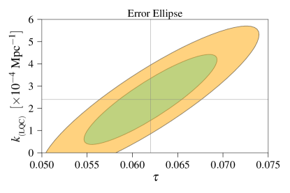
Figure 2: Error ellipse for $k_{{}_{\rm(LQC)}}$ and $\tau$. The inner and outer ellipses show 68 and 95% error contours respectively. The mean value is taken to be $k_{{}_{\rm(LQC)}}=0.00024~{}{\rm Mpc^{-1}}$ and the corresponding value of optical depth $\tau=0.062$ determined using the suppressed LQC PPS.

To quantify the aforementioned correlation $k_{{}_{\rm(LQC)}}$ and $\tau$, we compute the Fisher information matrix fisher . Since the Planck  data for low-$\ell$ polarization is not yet available, for this analysis we will assume that the error bars on $C_{\ell}^{\rm EE}$ at low-$\ell$’s is given by the cosmic variance limit. As discussed in tegmarkfisher , the Fisher matrix then takes the following form:

$$\mathbb{F}_{ij}=\sum_{\ell=2}^{\ell_{\rm max}}\frac{1}{\left(\Delta C_{\ell}^{\rm EE}\right)^{2}}~{}\frac{\partial C_{\ell}^{\rm EE}}{\partial\theta_{i}}\frac{\partial C_{\ell}^{\rm EE}}{\partial\theta_{j}},$$ (3)

where

$$\Delta C_{\ell}^{\rm EE}=\sqrt{\frac{2}{2\ell+1}}~{}C_{\ell}^{\rm EE},$$ (4)

and $\theta=\left(\tau,~{}k_{{}_{\rm(LQC)}}\right)$, while the other cosmological parameters are fixed at their best fit value given in planck15xiii . Recall that effects of $k_{{}_{\rm(LQC)}}$ are limited to very large angular scales and $\tau$ is determined from the E-mode reionization bump which also occurs at $\ell<20$. Therefore, we keep $\ell_{\rm max}$ in eq. (3) large enough (at least $50$) to include the affected multipoles in our analysis.

Elements of the covariance matrix between $k_{{}_{\rm(LQC)}}$ and $\tau$ are then obtained by inverting the Fisher matrix: $\mathbb{C}_{ij}=\left(\mathbb{F}^{-1}\right)_{\ij}$. Fig. 2 shows the error ellipse corresponding to $\mathbb{C}_{ij}$. The inner and outer contours correspond to the $68\%$ and $95\%$ confidence levels respectively. As expected from previous discussions, there is a strong degeneracy between $k_{{}_{\rm(LQC)}}$ and $\tau$. Note that $\mathbb{C}_{ij}$ only captures the information about the error bars and correlation between the two parameters. The mean values of $\tau$ and $k_{{}_{\rm(LQC)}}$ at which the errors ellipse is centered are given by the best fit values which we have obtained by proceeding as follows.

Implications for future observations and Constraints on LQC: As evident from Fig. 2, there is strong degeneracy between $k_{{}_{\rm(LQC)}}$ and $\tau$ measured from the low-$\ell$ polarization data. In order to break this degeneracy we would need an independent estimation of either $k_{{}_{\rm(LQC)}}$ or $\tau$. The LQC scale $k_{{}_{\rm(LQC)}}$ is a parameter of the underlying theory. On the other hand, $\tau$ can be measured using high-$\ell$ TT data as well as by upcoming experiments such as CMB S4 cmbs4 and 21 cm cosmology 21cmtau missions independent from Planck measurements. The measured value of $\tau$ from these experiments will break the degeneracy with $k_{{}_{\rm(LQC)}}$ and put observational constraints on $k_{{}_{\rm(LQC)}}$.

Recall that the value of $k_{{}_{\rm(LQC)}}$ determines $a(t_{\rm B})$, i.e. the initial conditions of the background geometry at the bounce. Thus, we can learn about the properties of quantum geometry using future observational data. Moreover, as discussed before, since the suppressed power determines a higher value of $\tau$, it can resolve the moderate discrepancy in the estimation of $\tau$ using the low-$\ell$ polarization and high-$\ell$ temperature data from Planck mission.

Re-estimating Optical Depth:

Figure 3: 1-dimensional posteriors of $\tau$ obtained with the “simulated” data for the standard PPS (dashed blue curve) and the suppressed LQC PPS (solid red curve) with $k_{{}_{\rm(LQC)}}=0.00024~{}{\rm Mpc^{-1}}$, which is chosen to represent the mean of the error ellipse in Fig. 2.

Note that, using the low-$\ell$ TT data in planck16xlvi , $\tau$ was determined to be $0.055$. Therefore, it is possible that if the suppressed power spectrum is used to determine $\tau$ with the low-$\ell$ EE data, the new value of $\tau$ might increase enough and come closer to $0.066$—the value obtained from high-$\ell$ TT data planck15xiii —hence resolving an apparent discrepancy between estimation of $\tau$ from low-$\ell$ EE and high-$\ell$ TT data. Let us find out if this expectation is borne out in our analysis.

To obtain the best fit values of $\tau$ for the suppressed PPS we perform the maximum likelihood analysis with low-$\ell$ $C_{\ell}^{\rm EE}$ by varying $\tau$, keeping $k_{{}_{\rm(LQC)}}=0.00024~{}{\rm Mpc^{-1}}$ (eq. (2)), obtained from consideration of simplest quantum geometry in the deep Planck regime ag3 , while fixing other cosmological parameters at their best fit values given in planck15xiii .

In order to perform this analysis, we need the EE spectrum measured from experiments at low-$\ell$ which, however, has not been made available publicly yet. Given the lack of real data, we will work with a “simulated” EE data at low-$\ell$ constructed in the following manner. We fix $\tau=0.055$ (i.e. the mean value of $\tau$ obtained in planck16xlvi ) and compute $C_{\ell}^{\rm EE}$ assuming the standard almost scale invariant power spectrum. We consider this to be the central values of $C_{\ell}^{\rm EE}$ with the errors bars given by the cosmic variance at low-$\ell$. In this sense, our “simulated” data represents the best ever possible CMB measurements at low multipoles.

Fig. 3 shows the corresponding one dimensional posterior distribution of $\tau$ for the standard PPS (dashed blue curve) and the suppressed LQC PPS (solid red curve). The estimated $\tau$ with $95\%$ error bars are:

$$\tau = 0.055\pm 0.008\qquad\qquad{\rm(Standard~{}PPS)}$$

$$\tau = 0.062\pm 0.008\qquad\qquad{\rm(Suppressed~{}PPS)}.$$ (5)

Note that the width of the posterior distribution is sharper as compared to that obtained in planck16xlvi , because here we have considered the “simulated” data with cosmic variance error bars which are significantly smaller. It is evident that the peak of the posterior has shifted to a higher value of $\tau$ when the suppressed power spectrum is used. Moreover, the re-estimated value is closer to the one obtained from high-$\ell$ TT data: $\tau=0.066$. This indicates that if the large scale power suppression is indeed a primordial effect rather than a statistical fluke, it can resolve the discrepancy between the estimation of $\tau$ purely from low-$\ell$ EE polarization spectrum (estimated to be $0.055$ with the standard PPS) and high-$\ell$ TT spectrum. This indicates further empirical support for the possibility that the PSA could have originated from physical processes in the very early Universe.

In this Letter we have shown that future observational data, in particualr giving independent measurement of $\tau$ can be used to determine the scale at which PSA is observed in the TT spectrum, which in turn can constrain the associated pre-inflationary physics. Here we have only presented a proof of principle that there is potentially a new window on pre-inflationary physics via a symbiotic interplay between observational data and fundamental. While we performed a case study by considering the pre-inflationary dynamics of loop quantum cosmology, the overall results of the analysis can be extended to other primordial mechanisms which introduces a characteristic scale for suppression of power at large angular scales. Due to the lack of availability of observational data for polarization at low-$\ell$ we used simulated data assuming the error bars on $C_{\ell}^{\rm EE}$ at low-$\ell$ to be given by the cosmic variance. The actual experimental data from Planck expected to be released in upcoming few months, will have higher error bars which is expected to only increase the width of the error ellipse while keeping the degeneracy intact. We will revisit this analysis when more data from Planck, CMB S4 and 21 cm cosmology is available, which hopefully will provide new observational insights on the physics of deep Planck regime in the very early Universe.

References

References

- (1) WMAP Collaboration, C. L. Bennett et al., “First year Wilkinson Microwave Anisotropy Probe (WMAP) observations: Preliminary maps and basic results”, Astrophys. J. Suppl. 148 (2003) 1–27, arXiv:astro-ph/0302207.
- (2) Planck Collaboration, P. A. R. Ade et al., “Planck 2015 results. XVI. Isotropy and statistics of the CMB”, Astron. Astrophys. 594 (2016) A16, arXiv:1506.07135.
- (3) D. J. Schwarz, C. J. Copi, D. Huterer, and G. D. Starkman, “CMB Anomalies after Planck”, Class. Quant. Grav. 33 (2016), no. 18, 184001, arXiv:1510.07929.
- (4) S. Das and T. Souradeep, “Suppressing CMB low multipoles with ISW effect”, JCAP 1402 (2014) 002, arXiv:1312.0025.
- (5) CMB-S4 Collaboration, K. N. Abazajian et al., “CMB-S4 Science Book, First Edition”, arXiv:1610.02743.
- (6) A. Liu, J. R. Pritchard, R. Allison, A. R. Parsons, U. Seljak, and B. D. Sherwin, “Eliminating the optical depth nuisance from the CMB with 21 cm cosmology”, Phys. Rev. D93 (2016), no. 4, 043013, arXiv:1509.08463.
- (7) Planck Collaboration, N. Aghanim et al., “Planck intermediate results. XLVI. Reduction of large-scale systematic effects in HFI polarization maps and estimation of the reionization optical depth”, Astron. Astrophys. 596 (2016) A107, arXiv:1605.02985.
- (8) Planck Collaboration, R. Adam et al., “Planck intermediate results. XLVII. Planck constraints on reionization history”, Astron. Astrophys. 596 (2016) A108, arXiv:1605.03507.
- (9) Planck Collaboration, P. A. R. Ade et al., “Planck 2015 results. XIII. Cosmological parameters”, Astron. Astrophys. 594 (2016) A13, arXiv:1502.01589.
- (10) WMAP Collaboration, A. Kogut et al., “Wilkinson Microwave Anisotropy Probe (WMAP) first year observations: TE polarization”, Astrophys. J. Suppl. 148 (2003) 161, arXiv:astro-ph/0302213.
- (11) WMAP Collaboration, J. Dunkley et al., “Five-Year Wilkinson Microwave Anisotropy Probe (WMAP) Observations: Likelihoods and Parameters from the WMAP data”, Astrophys. J. Suppl. 180 (2009) 306–329, arXiv:0803.0586.
- (12) WMAP Collaboration, G. Hinshaw et al., “Nine-Year Wilkinson Microwave Anisotropy Probe (WMAP) Observations: Cosmological Parameter Results”, Astrophys. J. Suppl. 208 (2013) 19, arXiv:1212.5226.
- (13) A. Ashtekar and B. Gupt, “Quantum Gravity in the Sky: Interplay between fundamental theory and observations”, Class. Quant. Grav. 34 (2017), no. 1, 014002, arXiv:1608.04228.
- (14) C. R. Contaldi, M. Peloso, L. Kofman, and A. D. Linde, “Suppressing the lower multipoles in the CMB anisotropies”, JCAP 0307 (2003) 002, arXiv:astro-ph/0303636.
- (15) J. M. Cline, P. Crotty, and J. Lesgourgues, “Does the small CMB quadrupole moment suggest new physics?”, JCAP 0309 (2003) 010, arXiv:astro-ph/0304558.
- (16) R. K. Jain, P. Chingangbam, J.-O. Gong, L. Sriramkumar, and T. Souradeep, “Punctuated inflation and the low CMB multipoles”, JCAP 0901 (2009) 009, arXiv:0809.3915.
- (17) L. Lello, D. Boyanovsky, and R. Holman, “Pre-slow roll initial conditions: large scale power suppression and infrared aspects during inflation”, Phys. Rev. D89 (2014), no. 6, 063533, arXiv:1307.4066.
- (18) F. G. Pedro and A. Westphal, “Low- CMB power loss in string inflation”, JHEP 04 (2014) 034, arXiv:1309.3413.
- (19) Y.-F. Cai, F. Chen, E. G. M. Ferreira, and J. Quintin, “New model of axion monodromy inflation and its cosmological implications”, JCAP 1606 (2016), no. 06, 027, arXiv:1412.4298.
- (20) A. Ashtekar and P. Singh, “Loop Quantum Cosmology: A Status Report”, Class. Quant. Grav. 28 (2011) 213001, arXiv:1108.0893.
- (21) I. Agullo, A. Ashtekar, and W. Nelson, “A Quantum Gravity Extension of the Inflationary Scenario”, Phys. Rev. Lett. 109 (2012) 251301, arXiv:1209.1609.
- (22) I. Agullo, A. Ashtekar, and W. Nelson, “The pre-inflationary dynamics of loop quantum cosmology: Confronting quantum gravity with observations”, Class. Quant. Grav. 30 (2013) 085014, arXiv:1302.0254.
- (23) B. Bonga and B. Gupt, “Phenomenological investigation of a quantum gravity extension of inflation with the Starobinsky potential”, Phys. Rev. D93 (2016), no. 6, 063513, arXiv:1510.04896.
- (24) A. Ashtekar, T. Pawlowski, and P. Singh, “Quantum nature of the big bang”, Phys. Rev. Lett. 96 (2006) 141301, arXiv:gr-qc/0602086.
- (25) R. A. Fisher, “The Fiducial Argument in Statistical Inference”, Annals Eugen. 6 (1935) 391–398.
- (26) M. Tegmark, A. Taylor, and A. Heavens, “Karhunen-Loeve eigenvalue problems in cosmology: How should we tackle large data sets?”, Astrophys. J. 480 (1997) 22, arXiv:astro-ph/9603021.
- (27) A. Ashtekar and B. Gupt, “Initial conditions for cosmological perturbations”, Class. Quant. Grav. 34 (2017), no. 3, 035004, arXiv:1610.09424.
- (28) M. Kamionkowski and A. Loeb, “Getting around cosmic variance”, Phys. Rev. D56 (1997) 4511–4513, arXiv:astro-ph/9703118.