Analysis of circulant embedding methods
for sampling stationary random fields

Abstract

A standard problem in uncertainty quantification and in computational statistics is the sampling of stationary Gaussian random fields with given covariance in a $d$-dimensional (physical) domain. In many applications it is sufficient to perform the sampling on a regular grid on a cube enclosing the physical domain, in which case the corresponding covariance matrix is nested block Toeplitz. After extension to a nested block circulant matrix, this can be diagonalised by FFT – the “circulant embedding method”. Provided the circulant matrix is positive definite, this provides a finite expansion of the field in terms of a deterministic basis, with coefficients given by i.i.d. standard normals. In this paper we prove, under mild conditions, that the positive definiteness of the circulant matrix is always guaranteed, provided the enclosing cube is sufficiently large. We examine in detail the case of the Matérn covariance, and prove (for fixed correlation length) that, as $h_{0}\rightarrow 0$, positive definiteness is guaranteed when the random field is sampled on a cube of size order $(1+\nu^{1/2}\log h_{0}^{-1})$ times larger than the size of the physical domain. (Here $h_{0}$ is the mesh spacing of the regular grid and $\nu$ the Matérn smoothness parameter.) We show that the sampling cube can become smaller as the correlation length decreases when $h_{0}$ and $\nu$ are fixed. Our results are confirmed by numerical experiments. We prove several results about the decay of the eigenvalues of the circulant matrix. These lead to the conjecture, verified by numerical experiment, that they decay with the same rate as the Karhunen–Loève eigenvalues of the covariance operator. The method analysed here complements the numerical experiments for uncertainty quantification in porous media problems in an earlier paper by the same authors in J. Comp. Physics. 230 (2011), pp. 3668–3694.

Keywords:

Gaussian Random Fields, Circulant Embedding, Statistical Homogeneity, Matérn Covariance, Fast Fourier Transform, Analysis

AMS:

60G10, 60G60, 65C05, 65C60

1 Introduction

In recent years there has been a huge growth in interest in uncertainty quantification (UQ) for physical models involving partial differential equations. In this context, the forward problem of UQ consists of describing the statistics of outputs (solutions) of a PDE model, given statistical assumptions on its inputs (e.g., its coefficients). This has led to the widespread study of model PDE problems where the coefficients are given as random fields. Various flavours of solution method (e.g., Stochastic Galerkin or various sampling methods) have been formulated under the assumption that the random coefficient field has a separable expansion in physical/probability space – for example a suitably truncated Karhunen–Loéve (KL) expansion, [10], [18].

In its standard form, the KL expansion is in principle infinite, and requires the computation of the (infinitely many) eigenpairs of the integral operator with kernel given by the covariance of the field. It has to be truncated to be computable, even when the field is only required at a finite set of physical spatial points. However if it is known from the outset that the coefficient field is only required at a finite set of physical points (as is the case in typical implementations of finite element methods for solving the PDE), then a different point of view emerges. The required field is now a random vector; in the Gaussian case it is characterised by its mean and covariance matrix. A real, for example Cholesky, factorization of the covariance matrix provides a finite separable expansion of the random vector, with no need for any truncation.

In the paper [11], the authors proposed a practical algorithm for solving a class of elliptic PDEs with coefficients given by statistically homogeneous lognormal random fields with low regularity. Lognormal random fields are commonly used in applications, for example in hydrology (see, e.g., [19, 20] and the references there).

The PDE was solved by piecewise linear finite elements on a uniform grid. The stiffness matrix was obtained by an appropriate quadrature rule, with the field values at the quadrature points being obtained via a factorization of the covariance matrix using the circulant embedding technique described below. The method was found to be effective even for problems with high stochastic dimension, but [11] did not contain a convergence analysis of the algorithm. The main purpose of the present paper is to provide an analysis for the circulant embedding part of the algorithm of [11]. The analysis of the corresponding uncertainty quantification algorithm for the PDE is done in [12].

We consider here the fast evaluation of a Gaussian random field $Z({\boldsymbol{x}},\omega)$ with prescribed mean $\overline{Z}({\boldsymbol{x}})$ and covariance

$$r_{\mathrm{cov}}({\boldsymbol{x}},{\boldsymbol{x}}^{\prime})\,:=\,\mathbb{E}[(Z({\boldsymbol{x}},\cdot)-\overline{Z}({\boldsymbol{x}}))(Z({\boldsymbol{x}}^{\prime},\cdot)-\overline{Z}({\boldsymbol{x}}^{\prime})],$$ (1.1)

where the expectation is with respect to the Gaussian measure. Throughout we will assume that $Z$ is stationary (see, e.g., [2, p. 24]), i.e., its covariance function satisfies

$$r_{\mathrm{cov}}({\boldsymbol{x}},{\boldsymbol{x}}^{\prime})\,=\,\rho({\boldsymbol{x}}-{\boldsymbol{x}}^{\prime}),$$ (1.2)

for some function $\rho:\mathbb{R}^{d}\to\mathbb{R}$. Note that we assume here that $\rho$ is defined on all of $\mathbb{R}^{d}$, as it is in many applications, although strictly speaking we only need $\rho$ to be defined on a sufficiently large ball. Note also that (1.1) and (1.2) imply that $\rho$ is symmetric, i.e.,

$$\rho({\boldsymbol{x}})=\rho(-{\boldsymbol{x}}),\quad\text{for all}\quad{\boldsymbol{x}}\in\mathbb{R}^{d}\ ,$$ (1.3)

and that $\rho$ is also positive semidefinite (see §2.2). Further assumptions on $\rho$ will be given below. A particular case, to be discussed extensively, is the Matérn covariance defined in Example 2.7 below.

We shall consider the problem of evaluating $Z({\boldsymbol{x}},\omega)$ at a uniform grid of

$$M\,=\,(m_{0}+1)^{d}$$

points on the $d$-dimensional unit cube $[0,1]^{d}$, with integer $m_{0}$ fixed, and with grid spacing $h_{0}:=1/m_{0}$. (The extension to general tensor product grids is straightforward and not discussed here.) Denoting the grid points by ${\boldsymbol{x}}_{1},{\boldsymbol{x}}_{2},\ldots,{\boldsymbol{x}}_{M}$, we wish to obtain samples of the random vector:

$${\boldsymbol{Z}}(\omega)\,:=\,(Z({\boldsymbol{x}}_{1},\omega),\ldots,Z({\boldsymbol{x}}_{M},\omega))^{\top}\ .$$

This is a Gaussian random vector with mean $\overline{{\boldsymbol{Z}}}:=(\overline{Z}({\boldsymbol{x}}_{1}),\ldots,\overline{Z}({\boldsymbol{x}}_{M}))^{\top}$ and a positive semidefinite covariance matrix

$$R\,=\,[\rho({\boldsymbol{x}}_{i}-{\boldsymbol{x}}_{j})]_{i,j=1}^{M}.$$ (1.4)

Because of its finite length, ${\boldsymbol{Z}}(\omega)$ can be expressed exactly (but not uniquely) as a linear combination of a finite number of i.i.d. standard normals, i.e., as

$${\boldsymbol{Z}}(\omega)\,=\,B\boldsymbol{Y}(\omega)\ +\ \overline{{\boldsymbol{Z}}}\ ,\quad\text{where}\quad\boldsymbol{Y}\sim\mathcal{N}(\boldsymbol{0},I_{s\times s}).$$ (1.5)

for some real $M\times s$ matrix $B$ with $s\geq M$ satisfying

$$R\,=\,BB^{\top}.$$ (1.6)

To verify this construction, simply note that (1.5) and (1.6) imply

$$\mathbb{E}[({\boldsymbol{Z}}-\overline{{\boldsymbol{Z}}})({\boldsymbol{Z}}-\overline{{\boldsymbol{Z}}})^{\top}]\,=\,\mathbb{E}[B\boldsymbol{Y}\boldsymbol{Y}^{\top}B^{\top}]\,=\,B\,\mathbb{E}[\boldsymbol{Y}\boldsymbol{Y}^{\top}]B^{\top}=BB^{\top}\,=\,R,$$

so ensuring that (1.1) is satisfied on the discrete grid.

In principle the factorization (1.6) could be computed via a Cholesky factorization (or even a spectral decomposition) of $R$ with $s=M$, but this is likely to be prohibitively expensive, since $R$ is large and dense. However, under appropriate ordering of the indices, $R$ is a nested block Toeplitz matrix and, as we will explain below, $R$ can be embedded in a bigger $s\times s$ nested block circulant matrix whose spectral decomposition can be rapidly computed using FFT with $\mathcal{O}(s\log s)$ complexity. A subtle but vital point is that while the covariance matrix $R$ is automatically positive semidefinite, the extension to a larger nested block circulant matrix may lose definiteness, yet the nested block circulant matrix must be at least positive semidefinite for the algorithm to work. Small deviations from positive semidefiniteness are acceptable if one is prepared to accept the incurred errors from omitted negative eigenvalues. That error can be controlled via an a posteriori bound in terms of the negative eigenvalues (see, e.g., [18, §6.5]). In the present paper, however, we insist on positive definiteness.

The principle of our extension of the covariance matrix $R$ is as follows. (Full details are in §2.1 below.) We first embed the unit cube $[0,1]^{d}$ in a larger cube $[0,{\ell}]^{d}$ with side length ${\ell}=mh_{0}\geq 1$ for some integer $m\geq m_{0}=1/h_{0}$. Note that $\rho$ is automatically defined on $[0,{\ell}]^{d}$, since it is defined on all of $\mathbb{R}^{d}$. Then we construct a $2{\ell}$-periodic even symmetric extension of $\rho$ on $[0,2{\ell}]^{d}$, called $\rho^{\mathrm{ext}}$, see (2.4) below, that coincides with $\rho$ on $[0,{\ell}]^{d}$. The extended $s\times s$ matrix with

$$s=(2m)^{d}$$ (1.7)

is then obtained by the analogue of formula (1.4), with $\rho$ replaced by $\rho^{\mathrm{ext}}$. In Theorem 2.3, we show, under quite general conditions, that if ${\ell}$ (equivalently $m$) is chosen large enough, this extension is necessarily positive definite. The algorithm used in practice (Algorithm 1 in §2 below) extends ${\ell}$ cautiously through a sequence of increments in $m$ until positive definiteness is achieved.

To know that the resulting algorithm is efficient, we need a lower bound on the value of ${\ell}$ needed to achieve positive definiteness. Our second set of theoretical results provides such bounds for the important Matérn class of covariance functions, defined in (2.21) below. In Theorem 2.9 we show that positive definiteness is always achieved with

$$\ell/\lambda\ \geq\ C_{1}\ +\ C_{2}\,\nu^{1/2}\,\log\left(\max\{{\lambda}/{h_{0}},\,\nu^{1/2}\}\right)\ ,$$ (1.8)

where $\lambda$ is a parameter with the unit of length (the “correlation length”), $\nu<\infty$ is the Matérn smoothness parameter and $C_{1},C_{2}$ are constants independent of $h_{0},{\ell},\lambda,\nu$ and variance $\sigma^{2}$. Thus the required ${\ell}$ grows very slowly in $1/h_{0}$ and can get smaller as the correlation length decreases. There is some growth as $\nu$ increases. However, the less smooth fields with $\nu$ small, and with small correlation length $\lambda$, are the ones often found in applications – see the references in [11]. In Theorem 2.11 we discuss the same question in the Gaussian case ($\nu=\infty$). This theorem shows, for example, that if $\lambda$ and $h_{0}$ both decrease but $\lambda/h_{0}$ is kept fixed (i.e., a fixed number of grid points per unit correlation length), then the minimum value of $\ell$ needed for positive definiteness can decrease linearly in $\lambda$.

An additional benefit of the spectral decomposition obtained by applying the FFT to the circulant matrix is that it allows us to determine empirically which variables are the most important in the system. This gives an ordering of the variables, which can be used to drive the design of the Quasi-Monte Carlo algorithms (see, e.g., [12]).

While circulant embedding techniques are well-known in the computational statistics literature (e.g., [5, 6, 7, 17, 18]), there is relatively little theoretical analysis of this technique, the best existing references being Chan and Wood [5] and Dietrich and Newsam [7]. First, [5] provides a theorem in general dimension $d$ identifying conditions on the covariance function which ensure that the circulant extension (which we shall describe below) is positive definite for some sufficiently large $\ell$. The condition is similar to that provided in our Theorem 2.3 below, except that an additional assumption on the discrete Fourier transform (the “spectral density”) of $\rho$ is required in [5]. In our work we require positivity of the continuous Fourier transform which is automatically satisfied via Bochner’s theorem, due to the fact that $\rho$ is a covariance kernel. On the other hand Dietrich and Newsam [7] provide more detailed information about the behaviour of the algorithm by restricting the theory to a 1-dimensional domain. They show that the discrete Fourier transform of $\rho$ will be positive when $r_{\rm cov}$ is convex, decreasing and non-negative. This automatically proves the success of the algorithm for certain covariance kernels. However, two covariance kernels that are not covered by this theory are the “Whittle” covariance and the Gaussian covariance. These belong to the Matérn class introduced in Example 2.7 below, with Matérn parameter $\nu=1$ and $\nu=\infty$ respectively. Our theory covers the whole Matérn family and also describes the behaviour of the embedding algorithm with respect to the parameters $\nu$ (Matérn parameter) and $\lambda$ (correlation length) as well as the mesh size $h_{0}$. Finally we note that [7] also describes embedding strategies which are more general than those which we describe and analyse here, but without theory.

We may compare the present approach with other methods for the generation of Gaussian random fields. The principal limitations of the present approach are that it requires the covariance function to be stationary, and generates the random field only on a uniform tensor product grid. The requirement of uniformity of the grid is not very restrictive for PDE applications, as we show in [12] where we take the interpolation error into account for the error analysis. In [9], the uniform grid requirement is removed but at the price of approximating the covariance matrix by an $H^{2}$-matrix, and then obtaining an approximate square root of that $H^{2}$-matrix. The use of $H$-matrices to promote the efficient computation of KL eigenfunctions has previously been explored in [8, 16, 14]. In [21], fast multipole methods were promoted to achieve the same objective. In all these approaches, there is an inevitable need to truncate the KL series, but on the other hand there is no essential restriction to stationary covariance functions. We mention also the recent paper [3] in which a related periodization procedure is applied (this time using a smooth cut-off function), facilitating wavelet expansions of $Z$.

An interesting paper closely related to the present paper is [14], where the authors propose and analyse an approximate, pivoted Cholesky factorisation followed by a small eigendecomposition, which provides in many cases a very efficient and accurate way to approximate the random field. This approach does not require stationarity or a uniform grid, but for efficiency reasons the factorisation needs to be truncated after $K\ll M$ steps, where in the simplest case $M$ is the number of grid points as in the present paper. For fixed $K$, the accuracy of the truncated expansion depends on the decay of the KL eigenvalues and the cost is $\mathcal{O}(K^{2}M)$. When the KL eigenvalues do not decay sufficiently fast, this limits the possible accuracy or leads to prohibitively high costs.

The structure of this paper is as follows. The circulant embedding algorithm is described in §2.1. The general theory of positive definiteness of the circulant extension of $R$ is given in §2.2. General isotropic covariances (of which the Matérn is an example) are studied in §2.3, with the estimate (1.8) proved in Theorem 2.9. A key ingredient in the theory of the related paper [12] is an estimate on the rate of decay of the eigenvalues of the the circulant extension of the original covariance matrix. We discuss this question in §3 where we prove several results about the eigenvalues of the circulant matrix, leading to the conjecture that they decay at the same rate as the Karhunen-Loève eigenvalues of the continuous field. Numerical experiments illustrating the theory are given in §4.

2 Circulant Embedding

There are potentially several ways of computing the factorization (1.6). Since $R$ is symmetric positive definite, its Cholesky factorization $R=LL^{\top}$ yields (1.6), with $s=M$. Alternatively, we can use the spectral decomposition $R=W\Lambda W^{\top}$, with $W$ being the orthogonal matrix of eigenvectors, and $\Lambda$ being the positive diagonal matrix of eigenvalues, again giving (1.6) with $s=M$, this time with $B=W\Lambda^{1/2}$. Given that the matrix $R$ is large and dense, in both of these cases the factorization will generally be expensive. In the present paper we use a spectral decomposition of a circulant extension of $R$ to obtain (1.6) with $s>M$ – see Theorem 2.2 below.

2.1 The extended matrix

Recall that we began with a uniform grid of points on the $d$-dimensional unit cube $[0,1]^{d}$. The $M=(m_{0}+1)^{d}$ points $\{{\boldsymbol{x}}_{i}:i=1,\ldots,M\}$ are assumed to have spacing $h_{0}:=1/m_{0}$ along each coordinate direction. We then consider an enlarged cube $[0,{\ell}]^{d}$ of edge length

$${\ell}:=mh_{0}\geq 1,$$ (2.1)

with integer $m\geq m_{0}$. We take the point of view that $m_{0}$ is fixed (and hence so too is $h_{0}$), while $m$ is variable (and hence so too is $\ell$).

We index the grid points on the unit cube by an integer vector ${\boldsymbol{k}}$, writing

$${\boldsymbol{x}}_{{\boldsymbol{k}}}\,:=\,h_{0}{\boldsymbol{k}}\qquad\text{for}\quad{\boldsymbol{k}}=(k_{1},\ldots,k_{d})\in\{0,\ldots,m_{0}\}^{d}.$$ (2.2)

Then it is easy to see that (with analogous vector indexing for the rows and columns) the $M\times M$ covariance matrix $R$ defined in (1.4) can be written as

$$R_{{\boldsymbol{k}},{\boldsymbol{k}}^{\prime}}\,=\,\rho\big{(}{h_{0}}({{\boldsymbol{k}}-{\boldsymbol{k}}^{\prime}})\big{)},\qquad{\boldsymbol{k}},{\boldsymbol{k}}^{\prime}\in\{0,\ldots,m_{0}\}^{d}.$$ (2.3)

If the vectors ${\boldsymbol{k}}$ are enumerated in lexicographical ordering, then $R$ is a nested block Toeplitz matrix where the number of nested levels is the physical dimension $d$. We remark that all indexing of matrices and vectors by vector notation in this paper is to be considered in this way.

In the following it will be convenient to extend the definition of the grid points (2.2) to an infinite grid,

$${\boldsymbol{x}}_{{\boldsymbol{k}}}\,:=\,h_{0}{\boldsymbol{k}}\qquad\text{for}\quad{\boldsymbol{k}}\in\mathbb{Z}^{d}.$$

Then, in order to define the extended matrix $R^{\mathrm{ext}}$, we define a $2{\ell}$-periodic map on $\mathbb{R}$ by specifying its action on $[0,2{\ell}]$:

$$\varphi(x)\,:=\,\begin{cases}x&\text{if}\quad 0\,\leq\,x\,\leq\,{\ell},\\ 2{\ell}-x&\text{if}\quad{\ell}\,\leq\,x\,<\,2{\ell}.\end{cases}$$

Now we apply this map componentwise and so define an extended version $\rho^{\mathrm{ext}}$ of $\rho$ as follows:

$$\rho^{\mathrm{ext}}({\boldsymbol{x}})\,:=\,\rho(\varphi(x_{1}),\ldots,\varphi(x_{d})),\qquad{\boldsymbol{x}}\in\mathbb{R}^{d}.$$ (2.4)

Note that $\rho^{\mathrm{ext}}$ is $2{\ell}$-periodic in each coordinate direction and

$$\rho^{\mathrm{ext}}({\boldsymbol{x}})\ =\ \rho({\boldsymbol{x}})\quad\text{when}\quad{\boldsymbol{x}}\in[0,{\ell}]^{d}.$$ (2.5)

Then $R^{\mathrm{ext}}$ is defined to be the $s\times s$ symmetric nested block circulant matrix with $s=(2m)^{d}$, defined, analogously to (2.3), by

$$R^{\mathrm{ext}}_{{\boldsymbol{k}},{\boldsymbol{k}}^{\prime}}\,=\,\rho^{\rm{ext}}\big{(}{h_{0}}({{\boldsymbol{k}}-{\boldsymbol{k}}^{\prime}})\big{)},\qquad{\boldsymbol{k}},{\boldsymbol{k}}^{\prime}\in\{0,\ldots,2m-1\}^{d}.$$ (2.6)

Moreover, $R$ is the submatrix of $R^{\mathrm{ext}}$ in which the indices are constrained to lie in the range ${\boldsymbol{k}},{\boldsymbol{k}}^{\prime}\in\{0,\ldots,m_{0}\}^{d}$.

In the following it will be convenient to introduce the notation, defined for any integer $m\geq 1$,

$$\mathbb{Z}_{2m}^{d}:=\{0,\ldots,2m-1\}^{d},\quad\quad\ {\overline{\mathbb{Z}}_{m}^{d}:=\{-m,\ldots,m-1\}^{d}}.$$

Then we have the following simple result.

Proposition 2.1

$R^{\mathrm{ext}}$ has real eigenvalues $\Lambda^{\mathrm{ext}}_{\boldsymbol{k}}$ and corresponding normalised eigenvectors ${\boldsymbol{V}}_{\boldsymbol{k}}$, given, for ${\boldsymbol{k}}\in{\mathbb{Z}}_{2m}^{d}$ by the formulae:

$$\Lambda^{\mathrm{ext}}_{\boldsymbol{k}}={\sum_{{\boldsymbol{k}}^{\prime}\in\overline{\mathbb{Z}}_{m}^{d}}}\rho({h_{0}{\boldsymbol{k}}^{\prime}})\exp\bigg{(}{-2\pi\mathrm{i}\frac{{\boldsymbol{k}}\cdot{\boldsymbol{k}}^{\prime}}{2m}}\bigg{)},\quad\text{and}\quad({\boldsymbol{V}}_{\boldsymbol{k}})_{{\boldsymbol{\kappa}}}=\frac{1}{\sqrt{s}}\exp\bigg{(}2\pi\mathrm{i}\frac{{\boldsymbol{k}}\cdot{\boldsymbol{\kappa}}}{2m}\bigg{)},\quad{\boldsymbol{\kappa}}\in{\mathbb{Z}}_{2m}^{d},$$ (2.7)

where $s$ is given in (1.7).

Proof.

By (2.4) and the fact that $\varphi$ is symmetric, we see that $\rho^{\mathrm{ext}}$ is also symmetric, so the eigenvalues of $R^{\mathrm{ext}}$ are real. To obtain the required formula for the eigenvalues, we use (2.6) and the formula for the eigenvectors in (2.7) to write, for ${\boldsymbol{k}},{\boldsymbol{\kappa}}\in\mathbb{Z}_{2m}^{d}$.

$$\left(R^{\mathrm{ext}}{\boldsymbol{V}}_{\boldsymbol{k}}\right)_{{\boldsymbol{\kappa}}}\ =\ \sum_{{\boldsymbol{k}}^{\prime}\in\mathbb{Z}_{2m}^{d}}\rho^{\mathrm{ext}}(h_{0}({\boldsymbol{\kappa}}-{\boldsymbol{k}}^{\prime}))\left({\boldsymbol{V}}_{\boldsymbol{k}}\right)_{{\boldsymbol{k}}^{\prime}}\ =\ \sum_{{\boldsymbol{k}}^{\prime\prime}\in{\boldsymbol{\kappa}}-\mathbb{Z}_{2m}^{d}}\rho^{\mathrm{ext}}(h_{0}\,{\boldsymbol{k}}^{\prime\prime})\left({\boldsymbol{V}}_{\boldsymbol{k}}\right)_{{\boldsymbol{\kappa}}-{\boldsymbol{k}}^{\prime\prime}}$$

$$=\ \Bigg{(}\sum_{{\boldsymbol{k}}^{\prime\prime}\in{\boldsymbol{\kappa}}-\mathbb{Z}_{2m}^{d}}\rho^{\mathrm{ext}}(h_{0}\,{\boldsymbol{k}}^{\prime\prime})\exp\left(-2\pi\mathrm{i}\frac{{\boldsymbol{k}}\cdot{\boldsymbol{k}}^{\prime\prime}}{2m}\right)\Bigg{)}\left({\boldsymbol{V}}_{\boldsymbol{k}}\right)_{{\boldsymbol{\kappa}}}.$$

Then (2.7) follows, on using the coordinatewise $2m$-periodicity of the summand in the last equation, and also the extension property (2.5). ∎

It follows from the simple form of the eigenfunctions that the matrix $R^{\mathrm{ext}}$ can be diagonalised by FFT. The following version of the spectral decomposition theorem, taken from [11], has the advantage that it allows the diagonalisation to be implemented using only real FFT.

Theorem 2.2

$R^{\mathrm{ext}}$ has the spectral decomposition:

$$\ R^{\mathrm{ext}}\ =\ Q^{\mathrm{ext}}\Lambda^{\mathrm{ext}}Q^{\mathrm{ext}},$$

where $\Lambda^{\mathrm{ext}}$ is the diagonal matrix containing the eigenvalues of $R^{\mathrm{ext}}$, and $Q^{\mathrm{ext}}=\mathfrak{Re}(\mathcal{F})+\mathfrak{Im}(\mathcal{F})$ is real symmetric, with

$$\mathcal{F}_{{\boldsymbol{k}},{\boldsymbol{k}}^{\prime}}=\frac{1}{\sqrt{s}}\exp\left({2\pi}\mathrm{i}\frac{{\boldsymbol{k}}^{\prime}\cdot{\boldsymbol{k}}}{{2m}}\right)$$

denoting the $d$-dimensional Fourier matrix. If the eigenvalues of $R^{\mathrm{ext}}$ are all non-negative then the required $B$ in (1.6) can be obtained by selecting $M$ appropriate rows of

$$B^{\mathrm{ext}}:=Q^{\mathrm{ext}}(\Lambda^{\mathrm{ext}})^{1/2}.$$ (2.8)

The use of FFT allows fast computation of the matrix-vector product $B^{\mathrm{ext}}{\boldsymbol{y}}$ for any vector ${\boldsymbol{y}}$, which then yields $B{\boldsymbol{y}}$ needed for sampling the random field in (1.5). Our algorithm for obtaining a minimal positive definite $R^{\mathrm{ext}}$ is given in Algorithm 1. Our algorithm for sampling an instance of the random field is given in Algorithm 2. Note that the normalisation used within the FFT routine differs among particular implementations. Here, we assume the Fourier transform to be unitary.

We can replace Step 1 of Algorithm 2 with a QMC point from $[0,1]^{s}$ and mapped to $\mathbb{R}^{s}$ elementwise by the inverse of the cumulative normal distribution function. The relative size of the eigenvalues in $\Lambda^{\mathrm{ext}}$ tells us the relative importance of the corresponding variables in the extended system, which helps to determine the ordering of the QMC variables.

Algorithm 1

Input: $d$, $m_{0}$, and covariance function $\rho$.

1. Set $m=m_{0}$.

2. Calculate ${\boldsymbol{r}}$, the first column of $R^{\mathrm{ext}}$ in (2.6).

3. Calculate ${\boldsymbol{v}}$, the vector of eigenvalues of $R^{\mathrm{ext}}$, by $d$-dimensional FFT on ${\boldsymbol{r}}$.

4. If smallest eigenvalue $<0$ then increment $m$ and go to Step 2.

Output: $m$, ${\boldsymbol{v}}$.

Algorithm 2

Input: $d$, $m_{0}$, mean field $\overline{Z}$, and $m$ and ${\boldsymbol{v}}$ obtained by Algorithm 1.

1. With $s=(2m)^{d}$, sample an $s$-dimensional normal random vector ${\boldsymbol{y}}$.

2. Update ${\boldsymbol{y}}$ by elementwise multiplication with $\sqrt{{\boldsymbol{v}}}$.

3. Set ${\boldsymbol{w}}$ to be the $d$-dimensional FFT of ${\boldsymbol{y}}$.

4. Update ${\boldsymbol{w}}$ by adding its real and imaginary parts.

5. Obtain ${\boldsymbol{z}}$ by extracting the appropriate $M=(m_{0}+1)^{d}$ entries of ${\boldsymbol{w}}$.

6. Update ${\boldsymbol{z}}$ by adding $\overline{Z}$.

Output: ${\boldsymbol{z}}$ (or $\exp({\boldsymbol{z}})$ in the case of lognormal field).

In the following subsection we shall show (under mild conditions) that Algorithm 1 will always terminate. Moreover we shall give (for the case of the Matérn covariance function) a detailed analysis of how ${\ell}$ depends on various parameters of the field. Then in §3, we give an analysis of the decay rates of the eigenvalues of $R^{\mathrm{ext}}$ compared with that of the the eigenvalues of the original Toeplitz matrix $R$ and the KL eigenvalues of the underlying continuous field $Z$.

2.2 Positive definiteness

We first note that by definition (1.1) and (1.2) it follows that for all $N\geq 1$, all point sets ${\boldsymbol{t}}_{1},\ldots,{\boldsymbol{t}}_{N}\in\mathbb{R}^{d}$, and all ${\boldsymbol{\gamma}}\in\mathbb{R}^{N}$

$$\sum_{i=1}^{N}\sum_{i^{\prime}=1}^{N}\gamma_{i}\,\gamma_{i^{\prime}}\,\rho({\boldsymbol{t}}_{i}-{\boldsymbol{t}}_{i^{\prime}})\ =\ \mathbb{E}[(W-\overline{W})^{2}]\ \geq\ 0,$$ (2.9)

where

$$W(\omega)=\sum_{i=1}^{N}\gamma_{i}Z({\boldsymbol{t}}_{i},\omega)$$

and $\overline{W}$ denotes its mean. This observation, together with (1.3), means that $\rho$ is a symmetric positive semidefinite function (see, e.g., [22, Chapter 6]). If in addition, (2.9) is always positive for nonzero ${\boldsymbol{\gamma}}$ then $\rho$ is called positive definite. In our later applications, $\rho$ will always be positive definite.

We use the following definition of the Fourier transform of an absolutely integrable function $\rho$:

$$\widehat{\rho}(\boldsymbol{\xi})\ =\ \int_{\mathbb{R}^{d}}\rho({\boldsymbol{x}})\,\exp(-2\pi\mathrm{i}\,\boldsymbol{\xi}\cdot{\boldsymbol{x}})\,\mathrm{d}{\boldsymbol{x}}\ ,\qquad\boldsymbol{\xi}\in\mathbb{R}^{d}\ .$$ (2.10)

If, in addition, $\rho$ is continuous and $\widehat{\rho}$ is absolutely integrable then the Fourier integral theorem gives

$$\rho({\boldsymbol{x}})\ =\ \int_{\mathbb{R}^{d}}\widehat{\rho}(\boldsymbol{\xi})\,\exp(2\pi\mathrm{i}\,\boldsymbol{\xi}\cdot{\boldsymbol{x}})\,\mathrm{d}\boldsymbol{\xi}\ ,\qquad{\boldsymbol{x}}\in\mathbb{R}^{d}\ .$$

In this case, $\widehat{\rho}$ is also continuous, and Bochner’s theorem (e.g., [18, Theorem 6.3]) states that $\rho$ is a positive definite function if and only if $\widehat{\rho}$ is positive.

The following theorem is the main result of this subsection.

Theorem 2.3

Suppose that $\rho\in L^{1}(\mathbb{R}^{d})$ is a real-valued, symmetric positive definite function with the additional reflectional symmetry

$$\rho({\boldsymbol{x}})=\rho(\pm x_{1},\ldots,\pm x_{d})=\rho(|x_{1}|,\ldots,|x_{d}|)\qquad\text{ for all }{\boldsymbol{x}}\in\mathbb{R}^{d},$$

and suppose $\widehat{\rho}\in L^{1}(\mathbb{R}^{d})$. Suppose also that for the given value of $h_{0}=1/m_{0}$ we have

$$\sum_{{\boldsymbol{k}}\in\mathbb{Z}^{d}}|\rho(h_{0}{\boldsymbol{k}})|\ <\ \infty.$$ (2.11)

Then Algorithm 1 will always terminate with a finite value of $m$, and the resulting matrix $R^{\rm{ext}}$ will be positive definite.

We prove Theorem 2.3 via a technical estimate – Lemma 2.4 – which provides an explicit lower bound for the eigenvalues of $R^{\mathrm{ext}}$. This estimate proves the theorem, and moreover, allows us to obtain explicit lower bounds for the eigenvalues in the lemmas which follow.

Lemma 2.4

Under the assumptions of Theorem 2.3, the eigenvalues $\Lambda^{\mathrm{ext}}_{\boldsymbol{k}}$ of $R^{\mathrm{ext}}$ all satisfy the estimate

$$\Lambda^{\mathrm{ext}}_{\boldsymbol{k}}\ \geq\ \frac{1}{h_{0}^{d}}\min_{{\boldsymbol{\zeta}}\in[-\frac{1}{2},\frac{1}{2}]^{d}}\sum_{{\boldsymbol{r}}\in\mathbb{Z}^{d}}\widehat{\rho}\Big{(}\frac{{\boldsymbol{\zeta}}+{\boldsymbol{r}}}{h_{0}}\Big{)}-\sum_{{\boldsymbol{k}}^{\prime}\in\mathbb{Z}^{d}\setminus\overline{\mathbb{Z}}_{m}^{d}}|\rho(h_{0}{\boldsymbol{k}}^{\prime})|\ .$$ (2.12)

Proof.

By Proposition  2.1, we have

$${\Lambda_{{\boldsymbol{k}}}^{\rm{ext}}} \,=\,\sum_{{\boldsymbol{k}}^{\prime}\in\mathbb{Z}^{d}}\rho\big{(}h_{0}{\boldsymbol{k}}^{\prime}\big{)}\exp\left(-{2\pi\mathrm{i}}\frac{{\boldsymbol{k}}^{\prime}\cdot{\boldsymbol{k}}}{2m}\right)-\sum_{{\boldsymbol{k}}^{\prime}\in\mathbb{Z}^{d}\setminus\overline{\mathbb{Z}}_{m}^{d}}\rho\big{(}h_{0}{\boldsymbol{k}}^{\prime}\big{)}\exp\left(-{2\pi\mathrm{i}}\frac{{\boldsymbol{k}}^{\prime}\cdot{\boldsymbol{k}}}{2m}\right).$$ (2.13)

We obtain the lower bound on the first sum on the right-hand side of (2.13) using (A.3) of Theorem A.1 in the Appendix with $h=h_{0}$ and $\boldsymbol{\xi}={\boldsymbol{k}}^{\prime}/(2m)$, and an upper bound on the second sum in the obvious way. ∎

• Because of the assumed positive definiteness of $\rho$, it follows from Bochner’s theorem that the Fourier transform $\widehat{\rho}$ is positive, so the strict positivity of the first term on the right-hand side of (2.12) follows from Theorem A.1. The lower bound is also independent of $m$. For fixed $h_{0}$, (2.11) ensures that the tail sum in the second term on the right-hand side of (2.12) converges to zero as $m\rightarrow\infty$. Hence the result follows. $\hfill\Box$

2.3 Isotropic covariance

More detailed lower bounds on $\Lambda^{\mathrm{ext}}_{{\boldsymbol{k}}}$ can be obtained under the additional assumption that the random field $Z$ in (1.1) is isotropic, i.e.,

$$\rho({\boldsymbol{x}})\,=\,\kappa(\|{\boldsymbol{x}}\|_{2}/\lambda)\ ,$$ (2.14)

where the parameter $\lambda$ is a correlation length which will play a key role in Example 2.7 and Theorem 2.9 below. In this case the Fourier transform (2.10) is given by

$$\widehat{\rho}(\boldsymbol{\xi})\,=\,\lambda^{d}\,\widehat{\kappa}_{d}({\lambda\|\boldsymbol{\xi}\|_{2}})\ ,$$ (2.15)

where

$$\widehat{\kappa}_{d}(r)\,:=\,\frac{2\pi}{r^{(d-2)/2}}\int_{0}^{\infty}\kappa(t)\,t^{d/2}\,J_{(d-2)/2}(2\pi\,rt)\,\mathrm{d}{t}\qquad\text{with }r\geq 0\ ,$$ (2.16)

and $J_{\alpha}$ denotes the Bessel function of order $\alpha$. The right-hand side of (2.16) is the Hankel transform of $\kappa$ (see, e.g., [18, Theorem 1.107]). The following lemma then estimates each of the terms on the right-hand side of (2.12) to obtain an explicit lower bound on the eigenvalues of $R^{\mathrm{ext}}$.

Lemma 2.5

Suppose $\rho$ and $\widehat{\rho}$ are given as in (2.14)–(2.16).

1. If $\,|\kappa|$ is a decreasing function on $\mathbb{R}_{+}$ and $\,r^{d-1}\,\kappa(r)\in L_{1}(\mathbb{R}_{+})$, then (with ${\ell}=mh_{0}$),

   $$\sum_{{\boldsymbol{k}}\in{\mathbb{Z}^{d}\setminus\overline{\mathbb{Z}}_{{}_{m}}^{d}}}|\rho(h_{0}{\boldsymbol{k}})|\,\leq\,\frac{(3^{d}-1)2^{d-1}}{(h_{0}/\lambda)^{d}}\int_{({\ell}-h_{0})/\lambda}^{\infty}r^{d-1}\,|\kappa(r)|\,\mathrm{d}r\,.$$

2. If $\widehat{\kappa}_{d}$ is positive and decreasing on $\mathbb{R}_{+}$ and $r^{d-1}\,\widehat{\kappa}_{d}(r)\in L_{1}(\mathbb{R}_{+})$, then

   $$\frac{1}{h_{0}^{d}}\min_{{\boldsymbol{\zeta}}\in[-\frac{1}{2},\frac{1}{2}]^{d}}\sum_{{\boldsymbol{r}}\in\mathbb{Z}^{d}}\widehat{\rho}\Big{(}\frac{{\boldsymbol{\zeta}}+{\boldsymbol{r}}}{h_{0}}\Big{)}\,\geq\,\frac{2^{d}}{d^{d/2-1}\,3^{d-1}}\int_{3d^{1/2}\lambda/(2h_{0})}^{\infty}r^{d-1}\,\widehat{\kappa}_{d}(r)\,\mathrm{d}r\,.$$

Proof.

We begin by deriving upper and lower bounds for some elementary sequences.

Suppose $g$ is any positive and decreasing function satisfying $r^{d-1}g(r)\in L_{1}(\mathbb{R}_{+})$. For any integer $m\geq 1$ we have

$$\sum_{j=m+1}^{\infty}j^{d-1}\,g(j)\leq\sum_{j=m+1}^{\infty}\int_{j-1}^{j}\left\lceil r\right\rceil^{d-1}\,g(r)\,\mathrm{d}{r}\leq\int_{m}^{\infty}(2r)^{d-1}\,g(r)\,\mathrm{d}{r},$$ (2.17)

where the first inequality uses $\left\lceil r\right\rceil=j$ for $r\in(j-1,j]$ and the second inequality follows from $\left\lceil r\right\rceil\leq 2r$ for $r\geq 1$. Similarly, we can obtain a lower bound for $m\geq 1$,

$$\sum_{j=m+1}^{\infty}j^{d-1}\,g(j)\geq\sum_{j=m+1}^{\infty}\int_{j}^{j+1}\left\lfloor r\right\rfloor^{d-1}\,g(r)\,\mathrm{d}{r}\geq\int_{m+1}^{\infty}(r/2)^{d-1}\,g(r)\,\mathrm{d}{r}.$$ (2.18)

Also let us consider the set $S_{d}(j):=\{{\boldsymbol{k}}\in\mathbb{Z}^{d}:\|{\boldsymbol{k}}\|_{\infty}=j\}$ for any integer $j\geq 1$. Then, with $\#\,S_{d}(j)$ denoting the cardinality of this set, we have the bounds

$$d\,2^{d}\,j^{d-1}\ \leq\ \#\,S_{d}(j)\ =\ (2j+1)^{d}-(2j-1)^{d}\ =\ 2\sum_{\begin{subarray}{c}i=1\\ i\text{ odd}\end{subarray}}^{d}\binom{d}{i}(2j)^{d-i}\ \leq\ (3^{d}-1)j^{d-1},$$ (2.19)

where the lower bound is the $i=1$ term in the binomial expansion and the upper bound comes from the estimate $j^{d-i}\leq j^{d-1}$ for $i\geq 1$. The bounds are exact for $d=1$ and $d=2$, with $\#\,S_{1}(j)=2$ and $\#\,S_{2}(j)=8j$, while for $d=3$ we have $\#S_{3}(j)=2+24j^{2}$, and the lower and upper bounds given by (2.19) are $24j^{2}$ and $26j^{2}$ respectively.

Now, to prove (i), using (2.19) and (2.17) and $\|{\boldsymbol{k}}\|_{2}\geq\|{\boldsymbol{k}}\|_{\infty}$, we can now write

$$\sum_{{\boldsymbol{k}}\in{\mathbb{Z}^{d}\setminus\overline{\mathbb{Z}}_{m}^{d}}} |\kappa(h_{0}\|{\boldsymbol{k}}\|_{2}/\lambda)|\,\leq\,\sum_{j=m}^{\infty}\sum_{\|{\boldsymbol{k}}\|_{\infty}=j}|\kappa(h_{0}\|{\boldsymbol{k}}\|_{2}/\lambda)|\,\leq\,(3^{d}-1)\sum_{j=m}^{\infty}\,j^{d-1}\,|\kappa(h_{0}j/\lambda)|$$

$$\,\leq\,(3^{d}-1)2^{d-1}\int_{m-1}^{\infty}r^{d-1}\,|\kappa(h_{0}r/\lambda)|\,\mathrm{d}r\,=\,\frac{(3^{d}-1)2^{d-1}}{(h_{0}/\lambda)^{d}}\int_{({\ell}-h_{0})/\lambda}^{\infty}r^{d-1}\,|\kappa(r)|\,\mathrm{d}r,$$

with ${\ell}=mh_{0}$, thus completing the proof of (i).

To prove (ii), note first that, for ${\boldsymbol{\zeta}}\in[-\frac{1}{2},\frac{1}{2}]^{d}$ and any ${\boldsymbol{r}}\in\mathbb{Z}^{d}$ with $\|{\boldsymbol{r}}\|_{\infty}=j$, we have $\|{\boldsymbol{\zeta}}+{\boldsymbol{r}}\|_{2}\leq d^{1/2}\|{\boldsymbol{\zeta}}+{\boldsymbol{r}}\|_{\infty}\leq d^{1/2}(1/2+j)$. Using (2.15), (2.19) and (2.18) and dropping the ${\boldsymbol{r}}={\boldsymbol{0}}$ term, we can write

$$\frac{1}{h_{0}^{d}}\sum_{{\boldsymbol{r}}\in\mathbb{Z}^{d}}\widehat{\rho}\Big{(}\frac{{\boldsymbol{\zeta}}+{\boldsymbol{r}}}{h_{0}}\Big{)}\ =\ \bigg{(}\frac{\lambda}{h_{0}}\bigg{)}^{d}\sum_{{\boldsymbol{r}}\in\mathbb{Z}^{d}}\widehat{\kappa}_{d}\Big{(}\frac{\lambda\|{\boldsymbol{\zeta}}+{\boldsymbol{r}}\|_{2}}{h_{0}}\Big{)}\ \geq\ \bigg{(}\frac{\lambda}{h_{0}}\bigg{)}^{d}\sum_{j=1}^{\infty}\sum_{\|{\boldsymbol{r}}\|_{\infty}=j}\widehat{\kappa}_{d}\Big{(}\frac{\lambda\|{\boldsymbol{\zeta}}+{\boldsymbol{r}}\|_{2}}{h_{0}}\Big{)}\\ \ \geq\ \frac{d\,2^{d}}{(h_{0}/\lambda)^{d}}\sum_{j=1}^{\infty}j^{d-1}\widehat{\kappa}_{d}\Big{(}\lambda\frac{d^{1/2}(1/2+j)}{h_{0}}\Big{)}\ \geq\ \frac{2d}{(h_{0}/\lambda)^{d}}\int_{1}^{\infty}r^{d-1}\widehat{\kappa}_{d}\Big{(}\frac{\lambda d^{1/2}(1/2+r)}{h_{0}}\Big{)}\,\mathrm{d}r\\ \ =\ \frac{2}{d^{d/2-1}}\int_{{3d^{1/2}\lambda/(2h_{0})}}^{\infty}\left(r-\frac{\lambda d^{1/2}}{2h_{0}}\right)^{d-1}\widehat{\kappa}_{d}(r)\,\mathrm{d}r\ \geq\ \frac{2}{d^{d/2-1}}\int_{{3d^{1/2}\lambda/(2h_{0})}}^{\infty}\left(\frac{2r}{3}\right)^{d-1}\widehat{\kappa}_{d}(r)\,\mathrm{d}r,$$

where the last inequality follows from $r-c\geq 2r/3\Leftrightarrow r\geq 3c$, with $c=d^{1/2}\lambda/(2h_{0})$. ∎

Corollary 2.6

Under the assumptions of Lemma 2.5, $R^{\mathrm{ext}}$ is positive definite if

$$\int_{3\lambda d^{1/2}/(2h_{0})}^{\infty}r^{d-1}\,\widehat{\kappa}_{d}(r)\,\mathrm{d}r\,>\,\frac{(3^{d}-1)\,3^{d-1}\,d^{d/2-1}}{2(h_{0}/\lambda)^{d}}\int_{({\ell}-h_{0})/\lambda}^{\infty}r^{d-1}\,|\kappa(r)|\,\mathrm{d}r.$$ (2.20)

Proof.

We make use of Lemma 2.4. The fact that $\rho\in L_{1}(\mathbb{R}^{d})$ and $\widehat{\rho}\in L_{1}(\mathbb{R}^{d})$ follow immediately from (2.14) and (2.16) respectively, and from the assumptions $r^{d-1}\kappa(r)\in L_{1}(\mathbb{R}^{+})$ and $r^{d-1}\widehat{\kappa}_{d}(r)\in L_{1}(\mathbb{R}^{+})$. It then follows from Part (i) of Lemma 2.5 that the assumption (2.11) of Theorem 2.3 is satisfied. Since the symmetry assumption in the theorem is automatically satisfied by an isotropic covariance, the result now follows immediately from Lemma 2.4. ∎

To interpret Corollary 2.6, recall that $\lambda$ is the correlation length, so $\lambda$ is bounded above (without loss of generality let us assume $\lambda\leq 1$), but $\lambda$ may approach $0$. If $h_{0}$ is chosen so that $h_{0}/\lambda$ is a fixed constant, then (2.20) and integrability of $r^{d-1}|\kappa(r)|$ ensures that positive definiteness is achieved for ${\ell}$ sufficiently large independently of $\lambda$ and $h_{0}$. The condition “$h_{0}/\lambda$ constant” is a natural analogue to the requirement in oscillatory problems that the meshwidth should be proportional to the wavelength. However if ${\ell}$ and $\lambda$ are fixed and $h_{0}\rightarrow 0$ (constituting “subwavelength mesh refinement” needed to get higher accuracy) we see that the sufficient condition that ensures positive definiteness will eventually fail. One interesting question is how fast ${\ell}$ needs to grow as $h_{0}$ decreases in order to be sure of positive definiteness. This can be answered fairly completely and satisfactorily in the case of the Matérn family.

Example 2.7

The Matérn family of covariances are defined by

$$\rho({\boldsymbol{x}})=\kappa(\|{\boldsymbol{x}}\|_{2}/\lambda)\ ,\quad\text{where}\quad\kappa(r)=\ \sigma^{2}\,\frac{2^{1-\nu}}{\Gamma(\nu)}(\sqrt{2\nu}\,r)^{\nu}K_{\nu}\left(\sqrt{2\nu}\,r\right).$$ (2.21)

Here $\Gamma$ is the gamma function and $K_{\nu}$ is the modified Bessel function of the second kind, $\sigma^{2}$ is the variance, $\lambda$ is the correlation length and $\nu>0$ is a smoothness parameter. The practically interesting range is $\nu\geq 1/2$, with the cases $\nu=1/2$ and $\nu=\infty$ corresponding to the exponential and Gaussian covariances respectively, see, e.g., [13]. For this reason, we have restricted the analysis to the case $\nu\geq 1/2$, see also Remark 2.10.

For this particular $\kappa$, the Hankel transform $\widehat{\kappa}_{d}$ (see (2.16)) is explicitly known, and so we have from (2.15)–(2.16) that

$$\widehat{\rho}(\boldsymbol{\xi})=\lambda^{d}\,\widehat{\kappa}_{d}(\lambda\|\boldsymbol{\xi}\|_{2})\ ,\quad\text{where}\quad\widehat{\kappa}_{d}(r)=\sigma^{2}2^{d}\pi^{d/2}(2\nu)^{\nu}\frac{\Gamma(\nu+d/2)}{\Gamma(\nu)}\,\frac{1}{(2\nu+(2\pi r)^{2})^{\nu+d/2}}\ .$$ (2.22)

(This can be obtained, for example, by some manipulation of the formula [18, p.264].) Note that for the Matérn case both $\rho$ and $\widehat{\rho}$ are positive, radial, decreasing functions.

The following theorem shows that when $\nu$ and $\lambda$ are fixed, ${\ell}$ needs to grow with order $\log h_{0}^{-1}$ in order to be sure of positive definiteness as $h_{0}\rightarrow 0$. On the other hand if $\lambda$ and $h_{0}$ are fixed, $\ell$ needs to grow like $\nu^{1/2}\log\nu$ as $\nu$ increases. For given $\ell$, $h_{0}$, the bound on $\ell$ gets smaller as $\lambda$ decreases. This provides conditions guaranteeing the termination of Algorithm 1.

Notation 2.8

When discussing the Matérn case, we shall use the notation $A\lesssim B$ (equivalently $B\gtrsim A$) to mean $A/B$ is bounded above independently of $\ell,h_{0},\lambda$ and $\nu$, and we write $A\sim B$ if $A\lesssim B$ and $B\lesssim A$.

Theorem 2.9

Consider the Matérn covariance family (2.21), with smoothness parameter $\nu$ satisfying $1/2\leq\nu<\infty$ and correlation length $\lambda\leq 1$. Suppose $h_{0}/\lambda\leq e^{-1}$. Then there exist positive constants $C_{1}$ and $C_{2}\geq 2\sqrt{2}$ which may depend on dimension $d$ but are independent of the other parameters $\ell,h_{0},\lambda,\nu,\sigma^{2}$, such that $R^{\mathrm{ext}}$ is positive definite if

$$\ell/\lambda\ \geq\ C_{1}\ +\ C_{2}\,\nu^{1/2}\,\log\left(\max\{{\lambda}/{h_{0}},\,\nu^{1/2}\}\right)\ .$$ (2.23)

Proof.

For convenience we introduce the notation

$$\Psi=\max\{{\lambda}/{h_{0}},\,\nu^{1/2}\}\ .$$

Aiming to verify (2.20), we note first that, since both $\kappa$ and $\hat{\kappa}_{d}$ depend linearly on $\sigma^{2}$, we can without loss of generality set $\sigma^{2}=1$. We shall obtain the following lower bound on the left-hand side of (2.20):

$$\int_{3\lambda d^{1/2}/(2{h_{0}})}^{\infty}r^{d-1}\,\widehat{\kappa}_{d}(r)\,\mathrm{d}r \ \gtrsim\ \ \nu^{\nu+d/2-1}(4\pi^{2})^{-\nu}\Psi^{-2\nu}\ ,$$ (2.24)

and (subject to assumption (2.23)), the following upper bound on the integral on the right-hand side of (2.20):

$$\int_{(\ell-h_{0})/\lambda}^{\infty}r^{d-1}|\kappa(r)|\mathrm{d}r\ \lesssim\ 5^{\nu}\nu^{d/2-1}\exp\left(-\sqrt{\frac{\nu}{2}}\frac{\ell-h_{0}}{\lambda}\right)\ .$$ (2.25)

Since these estimates are rather technical, we defer their justification until the end of this proof. Thus, assuming (2.24) and (2.25) we see that there exists $D>0$, with $D$ independent of $\ell,h_{0},\lambda,\nu$, such that (2.20) holds if

$$\exp\left(-\sqrt{\frac{\nu}{2}}\frac{\ell-h_{0}}{\lambda}\right)\ \leq D\ \left(\frac{\nu}{20\pi^{2}}\right)^{\nu}\Psi^{-2\nu}\ .$$

Taking logs and rearranging, this is equivalent to

$$({\ell}-h_{0})/\lambda\ \geq\sqrt{2/\nu}\log{(1/D)}\ +\sqrt{2}\nu^{1/2}\log(20\pi^{2}/\nu)+2\sqrt{2}\nu^{1/2}\log\Psi\ .$$

The first term on the right-hand side is positive only when $D<1$, in which case it is sufficient to replace $\sqrt{2/\nu}$ by its maximum value $2$ (given that $\nu\geq 1/2$). Similarly, the second term is positive only when $\nu\leq 20\pi^{2}$, and in this case we have

$$\nu^{1/2}\log(20\pi^{2}/\nu)\ \leq\ \sqrt{20\pi^{2}}\,\log(40\pi^{2}).$$

Taking into account that $h_{0}/\lambda\leq e^{-1}$, we have thus demonstrated the sufficiency of a condition of the form (2.23). We now complete the proof by proving the technical estimates (2.24) and (2.25).

Proof of estimate (2.24):   Recalling that $\widehat{\kappa}_{d}$ is given by (2.22), we may use the following elementary result to bound the ratio of gamma functions if $d$ is even:

$$\frac{\Gamma(\nu+d/2)}{\Gamma(\nu)}\ =(\nu+d/2-1)\ldots(\nu+1)\nu\ \geq\ \nu^{d/2}.$$ (2.26)

If $d$ is odd then we may use

$$\frac{\Gamma(\nu+d/2)}{\Gamma(\nu)}\ =(\nu+d/2-1)\ldots(\nu+3/2)(\nu+1/2)\frac{\Gamma(\nu+1/2)}{\Gamma(\nu)}$$ (2.27)

$$\geq\ \nu^{(d-1)/2}\frac{\Gamma(\nu+1/2)}{\Gamma(\nu)}\geq\ \nu^{(d-1)/2}(\nu-1/2+1/4)^{1/2}\ \geq\ \nu^{(d-1)/2}\nu^{1/2}/\sqrt{2}\$$

for all $\nu\geq 1/2$, where in the penultimate step we use Kershaw’s inequality (see [15], equation (1.3))

$$\frac{\Gamma(x+1)}{\Gamma(x+r)}>\left(x+\frac{r}{2}\right)^{1-r}\quad\mbox{for }\ x>0,\quad 0<r<1,$$

with $r=1/2$ and $x=\nu-1/2$. (If $\nu=1/2$ the result is obtained by taking the limit $\nu\to 1/2+$ and using continuity.)

On using this lower bound in (2.22), we obtain

$$\widehat{\kappa}_{d}(r)\ \gtrsim\ (2\nu)^{\nu}\nu^{d/2}(2\nu)^{-(\nu+d/2)}(1+2\pi^{2}r^{2}/\nu)^{-(\nu+d/2)}\ \sim\ (1+2\pi^{2}r^{2}/\nu)^{-(\nu+d/2)}.$$

Now (for convenience), we introduce the notation

$$a=3\sqrt{d}/2,\quad\widetilde{\Psi}=\max\{\lambda a/h_{0},\sqrt{\nu/2\pi^{2}}\}.$$

Then the left-hand side of (2.20) can be estimated from below by:

$$\int_{\lambda a/h_{0}}^{\infty}r^{d-1}\,\widehat{\kappa}_{d}(r)\,\mathrm{d}r\ \gtrsim\ \int_{\lambda a/h_{0}}^{\infty}r^{d-1}\left(1+2\pi^{2}{r^{2}}/\nu\right)^{-(\nu+d/2)}\mathrm{d}r$$

$$\geq\ \int_{\widetilde{\Psi}}^{\infty}r^{d-1}\left(1+2\pi^{2}r^{2}/\nu\right)^{-(\nu+d/2)}\mathrm{d}r\ .$$

Now, noting that when $r\geq\widetilde{\Psi}$ we have $2\pi^{2}r^{2}/\nu\geq 1$, and so

$$\int_{\lambda a/h_{0}}^{\infty}r^{d-1}\,\widehat{\kappa}_{d}(r)\,\mathrm{d}r \geq\ \int_{\widetilde{\Psi}}^{\infty}r^{d-1}(4\pi^{2}r^{2}/\nu)^{-(\nu+d/2)}\mathrm{d}r$$

$$=\left(\frac{\nu}{4\pi^{2}}\right)^{\nu+d/2}\int_{\widetilde{\Psi}}^{\infty}r^{-2\nu-1}\mathrm{d}r\ \sim\ \nu^{\nu+d/2-1}(4\pi^{2})^{-(\nu+d/2)}\widetilde{\Psi}^{-2\nu}\ .$$

which yields (2.24), since $\widetilde{\Psi}\sim\Psi$.

Proof of estimate (2.25):   It is sufficient to prove this estimate wth $\ell-h_{0}$ on each side replaced by $\ell$. By definition (2.21) and the change of variable $r\mapsto(\sqrt{2/\nu})r$, we have

$$\int_{\ell/\lambda}^{\infty}r^{d-1}|\kappa(r)|\mathrm{d}r\ \sim\ \frac{1}{{\Gamma(\nu)}}\left(\frac{\nu}{2}\right)^{\nu+d/2}\int_{\sqrt{2/\nu}(\ell/\lambda)}^{\infty}r^{d+\nu-1}|K_{\nu}(\nu r)|\mathrm{d}r\ .$$ (2.28)

To obtain an estimate for the Bessel function on the right-hand side of (2.28), note first that by the hypotheses of this theorem, we have $h_{0}/\lambda\leq e^{-1}$ and $\nu\geq 1/2$. Now assume that (2.23) holds, with $C_{1}>0$ and $C_{2}>2\sqrt{2}$, both not yet fixed. Then

$$\ell/\lambda\ \geq\ C_{1}+C_{2}\nu^{1/2}\ \geq\ C_{1}+2\sqrt{2}\nu^{1/2}\ >\ 2\sqrt{2}\nu^{1/2}=\,4\sqrt{\nu/2},$$ (2.29)

and hence the range of integration in (2.28) is contained in $[4,\infty)$.

The uniform asymptotic estimate for $K_{\nu}(\nu r)$ given in [1, 9.7.8] implies that there exists a $\nu^{*}<\infty$ and a constant $C$ such that, for all $\nu\geq\nu^{*}$,

$$|K_{\nu}(\nu r)|\ \leq\ C\nu^{-1/2}\exp(-\nu r)\quad r\in[4,\infty).$$ (2.30)

We shall show that in fact such an inequality holds for all $\nu\geq 1/2$ and all $r\geq 4$. To this end, for $\nu\geq 1/2$, we introduce the quantity

$$c(\nu):=\|\exp(z)z^{1/2}K_{\nu}(z)\|_{L_{\infty}(2,\infty)},$$

The continuity of $K_{\nu}$ on $[2,\infty)$ and the order-dependent asymptotics of $K_{\nu}$ [1, 9.7.2] ensure that $c(\nu)<\infty$ for all $\nu<\infty$. It can also be shown, by appealing to the integral representation of the modified Bessel function, that $c(\nu)$ is continuous with respect to $\nu$ when $\nu\geq 1/2$, from which we deduce that $c^{*}:=\max_{[1/2,\nu^{*}]}c(\nu)<\infty\ .$ Now, for $1/2\leq\nu\leq\nu^{*}$ and $r\geq 4$ we have $\nu r\geq 2$ and

$$\exp(\nu r)\nu^{1/2}|K_{\nu}(\nu r)|\ =\ r^{-1/2}\left[\exp(\nu r)(\nu r)^{1/2}|K_{\nu}(\nu r)|\right]\ \leq\ \frac{1}{2}c(\nu)\ \leq\ \frac{1}{2}c^{*}\ .$$

This shows that the estimate (2.30) holds uniformly for all $r\geq 4$ and $\nu\geq 1/2$. Using this in (2.28) we then have

$$\int_{\ell/\lambda}^{\infty}r^{d-1}|\kappa(r)|\mathrm{d}r\ \lesssim\ \frac{1}{{\Gamma(\nu)}}\left(\frac{\nu}{2}\right)^{\nu+d/2}\nu^{-1/2}\int_{\sqrt{2/\nu}(\ell/\lambda)}^{\infty}r^{d-1+\nu}e^{-\nu r}\mathrm{d}r\ .$$ (2.31)

Now note that (2.29) implies that $\ell/\lambda\geq C_{2}\nu^{1/2}$, and hence $\sqrt{2/\nu}(\ell/\lambda)\geq\sqrt{2}C_{2}$, so we can choose $C_{2}$ a large enough constant independent of $\ell,h_{0},\lambda,\nu,\sigma^{2}$ so that $\sqrt{2/\nu}(\ell/\lambda)\geq 10$. Then, using the elementary inequality $xe\leq e^{x}$ which holds when $x\geq 1$, it follows that $(r/10)e\leq\exp(r/10)$ when $r\geq 10$. Hence for $r\geq\sqrt{2/\nu}(\ell/\lambda)\geq 10$, we have

$$r^{d-1+\nu}\ \leq\ \left(\frac{10}{e}\right)^{d-1+\nu}\exp\left(\frac{d-1+\nu}{10}r\right)\ \leq\left(\frac{10}{e}\right)^{d-1+\nu}e^{{\nu r}/{2}}\ ,$$

where in the last step we used $d-1\leq 2\leq 4\nu$. Inserting this into the right-hand side of (2.31), we get, after integration and some manipulation,

$$\int_{\ell/\lambda}^{\infty}r^{d-1}|\kappa(r)|\mathrm{d}r\ \lesssim\ \frac{1}{{\Gamma(\nu)}}\left(\frac{5\nu}{e}\right)^{\nu}\nu^{d/2-3/2}\exp\left(-\sqrt{\frac{\nu}{2}}\frac{\ell}{\lambda}\right)\ .$$

Stirling’s formula implies that $\Gamma(\nu)\nu^{1/2}e^{\nu}\ \sim\ \nu^{\nu}$ and the estimate (2.25) follows. ∎

Remark 2.10

The cases $\nu\geq 1/2$ in the Matérn family of covariances are of main interest in applications. In order to avoid further technicalities, we have restricted our attention to those cases in the proof and used the lower bound on $\nu$ several times in a non-trivial way. First of all it is used in the demonstration that estimates (2.23), (2.24) and (2.25) are sufficient to ensure the positive definiteness of $R^{\mathrm{ext}}$. Then it is used in the proofs of each of the estimates (2.24) and (2.25). The extension of Theorem 2.9 to $\nu\in(0,1/2)$ remains an open question.

To complete the theory of this section, we discuss the case $\nu=\infty$. In this case,

$$\rho({\boldsymbol{x}})=\kappa(\|{\boldsymbol{x}}\|_{2}/\lambda),\quad\text{with}\quad\kappa(r)=\sigma^{2}\exp(-r^{2}/2),$$

and an elementary calculation gives

$$\widehat{\rho}(\boldsymbol{\xi})=\sigma^{2}(2\pi)^{d/2}\lambda^{d}\exp(-2\pi^{2}\lambda^{2}\|\boldsymbol{\xi}\|_{2}^{2}).$$

For this (Gaussian) covariance it is well-known that the Karhunen-Loéve expansion converges exponentially (see, e.g., [21]), in which case it may be preferable to compute realisations of the field $Z$ via the KL expansion, rather than the method proposed here. Nevertheless the existing analysis can be applied to this case as we now show.

Theorem 2.11

For the Gaussian covariance (i.e., the Matérn kernel with $\nu=\infty$), there exists a constant $B$ (depending only on spatial dimension $d$) such that positive definiteness of $R^{\mathrm{ext}}$ is guaranteed when

$${\ell}\ \geq\ {1}\ +\ \lambda\max\left\{\sqrt{2}\frac{\lambda}{h_{0}},B\right\}\ .$$

Hence, if $\lambda/h_{0}$ is fixed (i.e., a fixed number of grid points per unit correlation length is used), then the $\ell$ required for positive definiteness decreases linearly with decreasing correlation length $\lambda$, until the minimal value $\ell=1$ is reached.

Proof.

As before, without loss of generality we set $\sigma^{2}=1$ and we make use of Corollary 2.6. The left-hand side of (2.20) is then

$$(2\pi)^{d/2}\int_{3\lambda d^{1/2}/(2h_{0})}^{\infty}\ r^{d-1}\exp(-2\pi^{2}r^{2})\,\mathrm{d}r\ =\ (2\pi)^{-d/2}\int_{c_{1}(\lambda/h_{0})}^{\infty}r^{d-1}\exp(-r^{2}/2)\,\mathrm{d}r,$$

with $c_{1}=3\pi\sqrt{d}>1$ . To make this quantity greater than the right-hand side of (2.20), we require

$$\int_{(\ell-h_{0})/\lambda}^{\infty}r^{d-1}\exp(-r^{2}/2)\,\mathrm{d}r\ <\ c_{2}\left(\frac{h_{0}}{\lambda}\right)^{d}\int_{c_{1}\lambda/h_{0}}^{\infty}r^{d-1}\exp(-r^{2}/2)\,\mathrm{d}r,$$

with $c_{2}={2d(2\pi d)^{-d/2}}{{(3^{d}-1)^{-1}\,3^{1-d}}}$. We shall show that there exists $B$ (depending only on $d$) such that

$$\int_{\ell/\lambda}^{\infty}r^{d-1}\exp(-r^{2}/2)\,\mathrm{d}r\ <\ c_{2}\left(\frac{h_{0}}{\lambda}\right)^{d}\int_{c_{1}\lambda/h_{0}}^{\infty}r^{d-1}\exp(-r^{2}/2)\,\mathrm{d}r,$$ (2.32)

when

$${\ell}\ \geq\ \lambda\max\left\{\sqrt{2}c_{1}\frac{\lambda}{h_{0}},B\right\}\ ,$$ (2.33)

and the statement of the theorem then follows, since $h_{0}\leq 1$.

To prove (2.32), we estimate its left-hand side by

$$\int_{\ell/\lambda}^{\infty}r^{d-1}\exp(-r^{2}/2)\,\mathrm{d}r\ \ \leq\ \exp(-\ell^{2}/4\lambda^{2})\int_{\ell/\lambda}^{\infty}r^{d-1}\,\exp(-r^{2}/4)\,\mathrm{d}r$$

$$\ =\ 2^{d/2}\exp(-\ell^{2}/4\lambda^{2})\int_{\ell/(\sqrt{2}\lambda)}^{\infty}r^{d-1}\,\exp(-r^{2}/2)\,\mathrm{d}r\ .$$ (2.34)

We now choose $B$ (depending only on $d$) to have the property that

$$\exp(-x^{2}/4)\,x^{d}\ \leq\ c_{2},\ \quad\text{when}\quad x\geq B.$$ (2.35)

Then if $\ell$ satisfies (2.33), we have

$$\ell/\lambda\ \geq\ B\quad\text{ and}\quad\ell/\lambda\ \geq\ \sqrt{2}c_{1}\lambda/h_{0}>\sqrt{2}\lambda/h_{0}.$$ (2.36)

Thus, using (2.35) and (2.36), we have

$$2^{d/2}\,\exp(-\ell^{2}/4\lambda^{2})\ \leq\ c_{2}\left(\sqrt{2}\lambda/\ell\right)^{d}\ <\ c_{2}\left(h_{0}/\lambda\right)^{d}\ .$$

Combining this with (2.34) and using the fact that $\ell/(\sqrt{2}\lambda)\geq c_{1}\lambda/h_{0}$ we obtain (2.32). ∎

3 Eigenvalue decay

In this section we return to the formula (1.5) for sampling the random field ${\boldsymbol{Z}}$. For the circulant embedding method, using the notation introduced above, we have

$${\boldsymbol{Z}}(\omega)\ =\ \sum_{{\boldsymbol{k}}\in\overline{\mathbb{Z}}_{m}^{d}}\mathbf{B}_{\boldsymbol{k}}Y_{\boldsymbol{k}}(\omega)+\overline{{\boldsymbol{Z}}},$$

where $Y_{\boldsymbol{k}}$ are i.i.d. standard normals, $\mathbf{B}_{\boldsymbol{k}}$ are the columns of the matrix $B$, and in this case $B$ is taken to be the appropriate $M$ rows of the matrix $B^{\mathrm{ext}}$, as described in Theorem 2.2. Recalling (2.8) and noting that every entry in $\mathfrak{Re}(\mathcal{F})+\mathfrak{Im}(\mathcal{F})$ is bounded by $\sqrt{2/s}$, it follows that

$$\|\mathbf{B}_{\boldsymbol{k}}\|_{\infty}\,\leq\,\sqrt{\frac{2\,\Lambda^{\rm ext}_{{\boldsymbol{k}}}}{s}},\quad{\boldsymbol{k}}\in\overline{\mathbb{Z}}_{m}^{d},$$

where $\Lambda^{\rm ext}_{{\boldsymbol{k}}}$ are the eigenvalues of the matrix $R^{\mathrm{ext}}$.

In Quasi-Monte Carlo (QMC) convergence theory (see for example [13], [12]) it is important to have good estimates for $\|\mathbf{B}_{\boldsymbol{k}}\|_{\infty}$. More precisely, arranging the $\Lambda^{\mathrm{ext}}_{\boldsymbol{k}}$ in non-increasing order, it is important to study the rate of decay of the resulting sequence. In order to obtain some insight into this question we first recall that the $\Lambda^{\mathrm{ext}}_{\boldsymbol{k}}$ depend on both the regular mesh diameter $h_{0}$ and the extension length $\ell$ or equivalently, on $h_{0}$ and $m$ (see (2.1)). Since $m={\ell}h_{0}^{-1}$, the dimension $s$ given by (1.7) then grows if either $h_{0}$ decreases or $\ell$ increases (or both). To indicate the dependence on these two parameters, in this section we write variously

$$\Lambda^{\mathrm{ext}}_{\boldsymbol{k}}\ =\Lambda^{\mathrm{ext}}_{\boldsymbol{k}}(h_{0},\ell)\ =\Lambda^{\mathrm{ext}}_{s,{\boldsymbol{k}}}.$$

In order to get insight into the asymptotic behaviour of $\Lambda^{\mathrm{ext}}_{\boldsymbol{k}}(h_{0},\ell)$, we study first the spectrum of the continuous periodic covariance integral operator defined by

$${\mathcal{R}}^{\rm ext}\,v({\boldsymbol{x}})\,:=\,\ \int_{[0,2{\ell}]^{d}}\rho^{\rm ext}({\boldsymbol{x}}-{\boldsymbol{x}}^{\prime})\,v({\boldsymbol{x}}^{\prime})\,\mathrm{d}{\boldsymbol{x}}^{\prime},\quad{\boldsymbol{x}}\in[0,2{\ell}]^{d}\ ,$$

where $\rho^{\mathrm{ext}}$ is defined in (2.4). This operator is a continuous analogue of the matrix $R^{\mathrm{ext}}$ defined in (2.6) and the eigenvalues of each are closely related as we shall discuss below.

The operator $\mathcal{R}^{\mathrm{ext}}$ is a compact operator on the space of $2{\ell}$-periodic continuous functions on $\mathbb{R}^{d}$, and so it has a discrete spectrum with the only accumulation point at the origin. Since $\mathcal{R}^{\mathrm{ext}}$ is a periodic convolution operator, it is easily verified that its eigenvalues and (normalised) eigenfunctions (which depend on $\ell$) are

$$\lambda^{\mathrm{ext}}_{{\boldsymbol{k}}}(\ell)\ =\ \int_{[0,2\ell]^{d}}\rho^{\mathrm{ext}}({\boldsymbol{x}})\exp\left(-{2\pi\mathrm{i}\,\boldsymbol{\xi}_{\boldsymbol{k}}\cdot{\boldsymbol{x}}}\right)\mathrm{d}{\boldsymbol{x}}\ =\ \int_{[-\ell,\ell]^{d}}\rho({\boldsymbol{x}})\exp\left(-{2\pi\mathrm{i}\,\boldsymbol{\xi}_{\boldsymbol{k}}\cdot{\boldsymbol{x}}}\right)\mathrm{d}{\boldsymbol{x}}$$ (3.1)

$$\text{and}\quad v_{\boldsymbol{k}}({\boldsymbol{x}})=(2\ell)^{-d/2}\exp(2\pi\mathrm{i}\,\boldsymbol{\xi}_{\boldsymbol{k}}\cdot{\boldsymbol{x}}),\quad\text{and where}\quad\boldsymbol{\xi}_{\boldsymbol{k}}={\boldsymbol{k}}/(2\ell)\quad\text{and}\quad{\boldsymbol{k}}\in\mathbb{Z}^{d}.$$

Here we used the fact that $\rho^{\rm{ext}}$ is $2\ell$-periodic and that $\rho^{\rm{ext}}$ and $\rho$ coincide on $[-\ell,\ell]^{d}$. The eigenvalues $\lambda^{\mathrm{ext}}_{\boldsymbol{k}}(\ell)$ are real but not necessarily positive, since $\rho^{\mathrm{ext}}$, unlike $\rho$, may not be positive definite (for the definition see §2.2).

The close relationship between the eigenvalues of the continuous operator and the matrix eigenvalues is shown by the following theorem.

Theorem 3.1

For fixed $\ell\geq 1$ and fixed ${\boldsymbol{k}}\in\overline{\mathbb{Z}}_{m}^{d}$, where $m=\ell/h_{0}$, the matrix eigenvalues $\Lambda^{\mathrm{ext}}_{{\boldsymbol{k}}}(h_{0},\ell)$, weighted by $h_{0}^{d}$, converge to $\lambda^{\mathrm{ext}}_{{\boldsymbol{k}}}(\ell)$ as $h_{0}\to 0$:

$$h_{0}^{d}\,\Lambda^{\mathrm{ext}}_{{\boldsymbol{k}}}(h_{0},\ell)\rightarrow\lambda^{\mathrm{ext}}_{\boldsymbol{k}}(\ell),\quad\text{as}\quad h_{0}\rightarrow 0.$$

Proof.

The formula for $\Lambda^{\mathrm{ext}}_{\boldsymbol{k}}(h_{0},\ell)$ given by (2.7), when weighted by $h_{0}^{d}$, can be seen as a rectangle rule approximation of the second integral defining $\lambda^{\mathrm{ext}}_{\boldsymbol{k}}(\ell)$ in (3.1), with grid spacing of $h_{0}$. Since the integrand in that integral is continuous, the convergence claim holds. ∎

From now on we restrict attention to the Matérn case (Example 2.7). Our first result shows that $\lambda^{\mathrm{ext}}_{\boldsymbol{k}}(\ell)$ is exponentially close to the full range Fourier transform $\widehat{\rho}(\boldsymbol{\xi}_{\boldsymbol{k}})$ (given in (2.10)), and this holds true uniformly in $\ell$ and ${\boldsymbol{k}}$.

Lemma 3.2

For the case of the Matérn kernel, we have

$$\left|\lambda^{\mathrm{ext}}_{\boldsymbol{k}}(\ell)-\widehat{\rho}(\boldsymbol{\xi}_{\boldsymbol{k}})\right|\ \lesssim\ \lambda^{d}5^{\nu}\nu^{d/2-1}\exp\left(-\sqrt{\frac{\nu}{2}}\frac{\ell}{\lambda}\right)\,,\quad\text{for all}\quad\ell\geq 1\quad\text{and}\quad{\boldsymbol{k}}\in\overline{\mathbb{Z}}_{m}^{d}.$$ (3.2)

Thus there exist positive constants $C_{3},C_{4}$ (independent of $h_{0},{\ell},\lambda$ and $\nu$), such that, for all $\varepsilon>0$ and all ${\boldsymbol{k}}\in\overline{\mathbb{Z}}_{m}^{d}$,

$$\left|\lambda^{\mathrm{ext}}_{\boldsymbol{k}}(\ell)-\widehat{\rho}(\boldsymbol{\xi}_{\boldsymbol{k}})\right|\ \leq\ \varepsilon,\quad\text{when}\quad\ell/\lambda\ \geq\ C_{3}\,\nu^{1/2}+C_{4}\,\nu^{-1/2}\log(1/\varepsilon).$$ (3.3)

Proof.

From (3.1), (2.10) and (2.21), it is easy to see that

$$\left|\lambda^{\mathrm{ext}}_{\boldsymbol{k}}(\ell)-\widehat{\rho}(\boldsymbol{\xi}_{\boldsymbol{k}})\right|\ \leq\ \int_{\|{\boldsymbol{x}}\|_{2}\geq{\ell}}|\rho({\boldsymbol{x}})|\,\mathrm{d}{\boldsymbol{x}}\sim\int_{\ell}^{\infty}r^{d-1}|\kappa(r/\lambda)|\,\mathrm{d}r\ =\ \lambda^{d}\int_{{\ell}/\lambda}^{\infty}r^{d-1}\kappa(r)\,\mathrm{d}r,$$

with $\kappa$ as in (2.21), and again we use Notation 2.8. Then, using (2.25), we obtain (3.2).

Forcing the right-hand side of (3.2) to be bounded above by $\varepsilon$, rearranging and taking logs, we obtain a sufficient condition of the form

$$\sqrt{\frac{\nu}{2}}\,\frac{{\ell}}{\lambda}\ \geq\ C_{*}+\log(1/\varepsilon)+d\log\lambda+\nu\log 5+(d/2-1)\log\nu,$$

for some parameter-independent constant $C_{*}$. Recalling that we assume $\lambda\leq 1$, and using $\nu\geq 1/2$ and $\log(\nu)/\nu\lesssim 1$, the sufficiency condition in (3.3) follows. ∎

With Lemma 3.2 in mind, we now discuss the asymptotic behaviour of $\widehat{\rho}(\boldsymbol{\xi}_{{\boldsymbol{k}}})$, by making use of the analytic formula (2.22). In order to define an appropriate ordering we make the following definition.

Definition 3.3 (Ordering of the integer lattice)

Since $\mathbb{Z}^{d}$ is countable we can write its elements as a sequence $\{{\boldsymbol{k}}(j):j=1,2,\ldots\}$, such that ${\boldsymbol{k}}(1)=\mathbf{0}\in\mathbb{Z}^{d}$ and such that the sequence $\{\|{\boldsymbol{k}}(j)\|_{2}:j=1,2,\ldots\}$ is non-decreasing. This ordering is not unique.

Theorem 3.4

For the case of the Matérn kernel, we have

$$0\ <\ \widehat{\rho}(\boldsymbol{\xi}_{{\boldsymbol{k}}(j)})\ \lesssim\ \lambda^{-2\nu}\ (\nu{\ell}^{2})^{\nu+d/2}\,j^{-(1+2\nu/d)},\quad j=1,2,\ldots\ .$$ (3.4)

Proof.

By (2.22) and the definition $\boldsymbol{\xi}_{\boldsymbol{k}}={\boldsymbol{k}}/(2\ell)$, we have

$$0\ <\ \widehat{\rho}(\boldsymbol{\xi}_{\boldsymbol{k}}) \ \sim\ \lambda^{d}\nu^{\nu}\,\frac{\Gamma(\nu+d/2)}{\Gamma(\nu)}\,\left(\nu+\pi^{2}\lambda^{2}\|{\boldsymbol{k}}\|_{2}^{2}/(2{\ell}^{2})\right)^{-(\nu+d/2)}.$$

Now by (2.26) we have (for even $d$), ${\Gamma(\nu+d/2)}\ \lesssim\ \nu^{d/2}\,{\Gamma(\nu)}$. Moreover the same estimate also holds for $d$ odd, as can be seen by employing the first equation in (2.27), and then the estimate $\Gamma(\nu+1/2)\ \lesssim\ \nu^{1/2}\Gamma(\nu)$ (from [15, eq. (1.3)]). Hence we have the upper bound

$$\widehat{\rho}(\boldsymbol{\xi}_{\boldsymbol{k}}) \ \lesssim\ \lambda^{d}\nu^{\nu+d/2}\,\left(\nu+\pi^{2}\lambda^{2}\|{\boldsymbol{k}}\|_{2}^{2}/(2{\ell}^{2})\right)^{-(\nu+d/2)}\ \lesssim\ \lambda^{d}\left(\nu\ell^{2}\right)^{\nu+d/2}(\lambda\|{\boldsymbol{k}}\|_{2})^{-(2\nu+d)}$$

$$\ =\ \lambda^{-2\nu}(\nu\ell^{2})^{\nu+d/2}\|{\boldsymbol{k}}\|_{2}^{-(2\nu+d)}.$$

Now, to complete the proof of (3.4), we shall show that

$$\|{\boldsymbol{k}}(j)\|_{2}\ \sim\ j^{1/d}\ .$$ (3.5)

To obtain (3.5), for each $j$, define the set $T(j):=\{{\boldsymbol{k}}\in\mathbb{Z}^{d}:\|{\boldsymbol{k}}\|_{2}\,\leq\,\|{\boldsymbol{k}}(j)\|_{2}\}$. Then $T(j)$ is a superset and a subset of two cubes:

$$[-d^{-1/2}\|{\boldsymbol{k}}(j)\|_{2},d^{-1/2}\|{\boldsymbol{k}}(j)\|_{2}]^{d}\ \subseteq\ T(j)\ \subseteq\ [-\|{\boldsymbol{k}}(j)\|_{2},\|{\boldsymbol{k}}(j)\|_{2}]^{d}\ .$$

(The right inclusion follows from the definition of $T(j)$. On the other hand if ${\boldsymbol{k}}$ lies in the left-most cube, then $\|{\boldsymbol{k}}\|_{\infty}\leq d^{-1/2}\|{\boldsymbol{k}}(j)\|_{2}$ which implies $\|{\boldsymbol{k}}\|_{2}\leq\|{\boldsymbol{k}}(j)\|_{2}$, i.e., ${\boldsymbol{k}}\in T(j)$.) Then it follows that $\#T(j)\,\sim\,\|{\boldsymbol{k}}(j)\|_{2}^{d}$. But also by definition $T(j)$ contains $j-1$ elements of $\mathbb{Z}^{d}$. Hence (3.5) follows. ∎

Combining Lemma 3.2 and Theorem 3.4 with Theorem 2.9, we obtain the following criterion which simultaneously guarantees the positivity of all the eigenvalues of $R^{\mathrm{ext}}$ and provides an upper bound for $\lambda_{{\boldsymbol{k}}(j)}(\ell)$, explicit in the parameters $h_{0},\ell,\lambda$ and $\nu$.

Corollary 3.5

For the Matérn kernel, suppose

$$\ell/\lambda\ \geq\ \max\{C_{1},C_{3}\nu^{1/2}\}\,+\max\{C_{2}\nu^{1/2},C_{4}\nu^{-1/2}\}\log\left(\max\{\lambda/h_{0},\nu^{1/2}\}\right).$$

Then $\Lambda^{\mathrm{ext}}_{{\boldsymbol{k}}}(h_{0},\ell)\geq 0$ for all ${\boldsymbol{k}}\in\overline{\mathbb{Z}}_{m}^{d}$ and also

$$\lambda^{\mathrm{ext}}_{{\boldsymbol{k}}(j)}(\ell)\ \leq\ \min\{h_{0}/\lambda,\nu^{-1/2}\}\ +\ \lambda^{-2\nu}\ (\nu{\ell}^{2})^{\nu+d/2}\,j^{-(1+2\nu/d)},\quad j=1,2,\ldots\$$ (3.6)

Discussion 3.6

In the paper [12] the authors of this paper analyse the convergence of Quasi-Monte Carlo methods for uncertainty quantification of certain PDEs with random coefficients, realisations of which are computed using the circulant embedding technique described here. A dimension-independent convergence estimate for the QMC method is proved there under the assumption that given $d$ and covariance function $\rho$, there exist $p<1$ and $C>0$ such that for all integers $m_{0}$, with $m$ chosen as in Algorithm 1 and $s=(2m)^{d}$, we have

$$\sum_{{\boldsymbol{k}}\in{\overline{\mathbb{Z}}_{m}^{d}}}\bigg{(}\frac{\Lambda^{\rm ext}_{s,{\boldsymbol{k}}}}{s}\bigg{)}^{p/2}\ \leq\ C\ .$$ (3.7)

If $\Lambda^{\mathrm{ext}}_{s,j}$ for $j=1,\ldots,s$ denotes the eigenvalues $\Lambda^{\mathrm{ext}}_{s,{\boldsymbol{k}}}$ reordered so as to be nonincreasing, then a sufficient condition for this to hold is that for some $\beta>1$ and $C>0$, independent of $j$ and $s$, there holds

$$\sqrt{\frac{\Lambda^{\rm ext}_{s,j}}{s}}\leq Cj^{-\beta}\quad\text{for}\quad j=1,\ldots,s,$$ (3.8)

in which case (3.7) holds for $p$ any number in the open interval $(1/\beta,1)$. Based on the known rate of decay of the analogous Karhunen-Loève eigenvalues (e.g., [18], [13]) and the fact that the second term in (3.6) decays with the same rate (and bearing in mind the result of Theorem 3.1), we conjecture that

$$\mbox{{Conjecture}:\quad For the Mat\'{e}rn\ kernel, \ \eqref{eq:decay_beta} holds with}\quad\beta=\frac{1+2\nu/d}{2}\ .$$ (3.9)

Numerical experiments in the next section support this conjecture. Thus we need to assume that $\nu>d/2$ in order to ensure that $\beta>1$ and $p<1$. (If $\nu\leq d/2$ then there is no predicted convergence rate for the QMC algorithm. A similar theoretical barrier was detected in [13]).

The conjecture that $\sqrt{\Lambda^{\rm ext}_{s,j}/s}\leq Cj^{-(1+2\nu/d)/2}$ remains a conjecture in spite of the results in Lemma 3.2 and Theorem 3.4. That is because these results concern the continuous eigenvalues $\lambda^{\mathrm{ext}}_{{\boldsymbol{k}}}(\ell)$ and the result which connects these with the eigenvalues $\Lambda^{\mathrm{ext}}_{{\boldsymbol{k}}}(h_{0},\ell)$ (namely Theorem 3.1) does not provide enough information about the small eigenvalues. Indeed it is well known, and demonstrated in the numerical experiments in the next section, that the small matrix eigenvalues depart significantly from the corresponding eigenvalues $\lambda^{\rm{ext}}_{{\boldsymbol{k}}}(\ell)$ of the integral operator.

A sufficient condition for (3.8), and hence for (3.7), is that (3.8) holds not for all eigenvalues but for some fixed fraction of the eigenvalues, say $\alpha$, starting from the largest. Suppose, for example, that for some fixed $\alpha\in(0,1)$ we have

$${\sqrt{\frac{\Lambda^{\rm ext}_{s,j}}{s}}}\leq Cj^{-\beta}\quad\text{for}\quad j=1,\ldots,\lceil\alpha s\rceil.$$

Then because the eigenvalues are ordered, we also have, for $j=\lceil\alpha s\rceil+1,\ldots,s$,

$${\sqrt{\frac{\Lambda^{\rm ext}_{s,j}}{s}}}\leq C\lceil\alpha s\rceil^{-\beta}\ =Cj^{-\beta}\left(\frac{j}{\lceil\alpha s\rceil}\right)^{\beta}\leq\frac{C}{\alpha^{\beta}}j^{-\beta},$$

so that the sufficiency condition (3.8) is satisfied for all $j=1,\dots,s$ with an appropriately larger value of the constant.

4 Numerical Experiments

In this section we perform numerical experiments illustrating the theoretical results given above, for the Matérn covariance in 2D and 3D. In all experiments we set the variance $\sigma^{2}=1$. In §4.1, we illustrate the positive definiteness results of Theorem 2.9. Then, in §4.2, we illustrate the actual decay of the eigenvalues $\Lambda^{\mathrm{ext}}_{s,j}$ and compare it to (3.9).

4.1 Positive definiteness

We investigate experimentally the minimal value of $\ell$ needed to ensure that the extended circulant matrix $R^{\mathrm{ext}}$ is positive definite. Recall that Theorem 2.3 guarantees the existence of such an $\ell$ and Theorems 2.9 and 2.11 quantify its behaviour in the Matérn case.

The plots in Figure 1 show the behaviour of $\ell$ as a function of $\log h_{0}^{-1}=\log m_{0}$ for various choices of $d$, $\nu<\infty$ and $\lambda$. They clearly show that $\ell$ depends linearly on $\log m_{0}$, for $m_{0}$ large enough. They also indicate that $\ell$ gets smaller if either $\lambda$ or $\nu$ gets smaller, all in accordance with Theorem 2.9. For fixed $d$, $h_{0}$ and $\lambda$, Theorem 2.9 gives a lower bound on $\ell$ which grows like $\nu^{1/2}$. We observe this behaviour clearly for $d=2$, but the growth with respect to $\nu$ is a bit slower for $d=3$. (See Figure 2, which plots $\log\ell$ against $\log\nu$.) The small triangle embedded in each graph indicates $\mathcal{O}(\nu^{1/2})$ growth.

$\lambda$	$m_{0}$	$\ell$ ($d=2$)	$\ell$ ($d=3$)
$1$	$8$	$8$	$9$
$0.5$	$16$	$4$	$4.5$
$0.25$	$32$	$2$	$2.25$
$0.125$	$64$	$1$	$1.125$

Table 1: Illustration of Theorem 2.11: Values of $\ell$ required to ensure positive definiteness of $R^{\mathrm{ext}}$ in the case $\nu=\infty$, with $\lambda$ decreasing and $m_{0}\lambda=8$ fixed.

Table 1 illustrates the result of Theorem 2.11 which covers the case $\nu=\infty$. Here we tabulate the value of $\ell$ needed to ensure positive definiteness of $R^{\mathrm{ext}}$, when decreasing $\lambda$ and keeping $m_{0}\lambda$ fixed at $8$. Theorem 2.11 gives a bound which decreases linearly in $\lambda$, until the minimum $\ell=1$ is reached. This behaviour is exactly as observed in Table 1. In this case $R^{\mathrm{ext}}$ has many very small eigenvalues and we deem it to be positive definite when all eigenvalues are positive, ignoring those eigenvalues which are less than $10^{-13}$ in modulus.

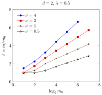
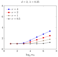
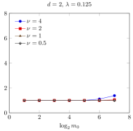
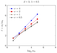
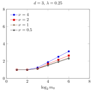
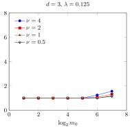
Figure 1: Illustration of Theorem 2.9: Graphs of the minimum needed value of $\ell$ to obtain positive definiteness against $\log_{2}h_{0}^{-1}=\log_{2}m_{0}$ for different choices of $d$, $\lambda$ and $\nu$. The graphs show a linear relationship with lower values of $\ell$ for smaller $\lambda$ and for smaller $\nu$.

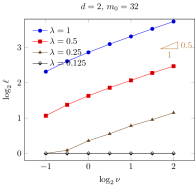
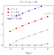
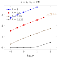
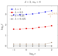
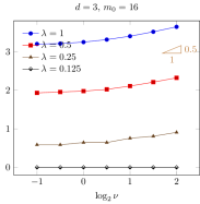
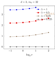
Figure 2: Illustration of Theorem 2.9: Log-log graphs of the minimum needed value of $\ell$ to obtain positive definiteness against $\nu$ for various choices of $d$, $m_{0}$ and $\lambda$. The small triangle depicts a gradient of $0.5$.

4.2 Eigenvalue decay

Here we perform experiments to verify the decay conjecture (3.9). In Figures 3 and 4 we present log-log plots of $\sqrt{\Lambda^{\mathrm{ext}}_{s,j}/s}$ against the index $j$ for various choices of $d$, $\nu$ and $\lambda$. For decreasing $h_{0}$ (i.e., increasing $m_{0}$) we determine the minimum $\ell$ to achieve positive definiteness and make the plot for each case. If the conjecture (3.9) holds, then we expect to see a polynomial decay of rate $-(1+2\nu/d)/2$, as shown in the slope triangle in each case. (The convergence may tail off eventually; note that Theorem 3.1 does not provide an explicit convergence rate.) We see that the computations closely follow the prediction of (3.9). Moreover, to have the constant $C$ in (3.7) for the minimal embedding to be absolutely bounded independent of $h_{0}$ (and thus also independent of $s$, $m$ and $\ell$) we observe the lines to get closer together for increasing $m_{0}$.

Thus, while the numerical evidence supports conjecture (3.9), it remains an interesting open problem to prove it.

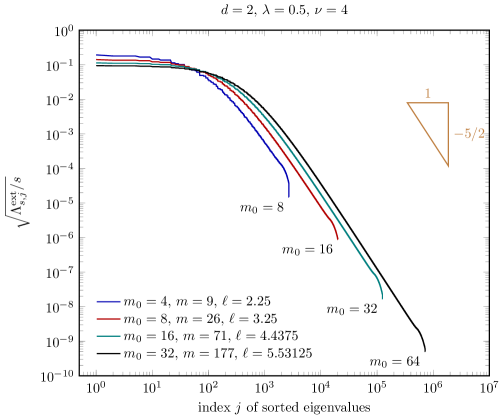
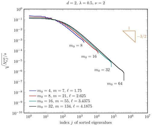
Figure 3: Loglog plot of the decay of the eigenvalues in case of the minimal embedding for $d=2$, $\lambda=0.5$, and $\nu=4$ (top) and $\nu=2$ (bottom). The expected decay rates (3.9) are marked by the slope triangles.

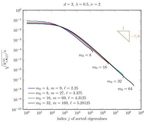
Figure 4: Loglog plot of the decay of the eigenvalues in case of the minimal embedding for $d=3$, $\lambda=0.5$ and $\nu=2$. The expected decay rate (3.9) is marked by the slope triangle.

Appendix A Sampling theorem

The following result is a $d$-dimensional version of what is commonly called a sampling theorem. (See [4] for a $1$-dimensional version.)

Theorem A.1

Let $\rho\in L^{1}(\mathbb{R}^{d})$ be real-valued and symmetric, with $\widehat{\rho}\in L^{1}(\mathbb{R}^{d})$. Suppose also that for some ${h}>0$,

$$\sum_{{\boldsymbol{k}}\in\mathbb{Z}^{d}}|\rho(h{\boldsymbol{k}})|<\infty.$$ (A.1)

Then

$$\sum_{{\boldsymbol{k}}\in\mathbb{Z}^{d}}\rho({h}{\boldsymbol{k}})\,\exp(-2\pi\mathrm{i}{h}{\boldsymbol{k}}\cdot\boldsymbol{\xi}) \,=\,\frac{1}{{h}^{d}}\sum_{{\boldsymbol{r}}\in\mathbb{Z}^{d}}\widehat{\rho}\left(\boldsymbol{\xi}+\frac{{\boldsymbol{r}}}{{h}}\right)\qquad\text{for {almost} all }\boldsymbol{\xi}\in\mathbb{R}^{d}.$$ (A.2)

If $\widehat{\rho}$ is everywhere positive, then for all $\boldsymbol{\xi}\in\mathbb{R}^{d}$

$$\sum_{{\boldsymbol{k}}\in\mathbb{Z}^{d}}\rho(h{\boldsymbol{k}})\,\exp(-2\pi\mathrm{i}h{\boldsymbol{k}}\cdot\boldsymbol{\xi})\, \geq\,\mathrm{essinf}_{{\boldsymbol{\zeta}}\in[-\frac{1}{2h},\frac{1}{2h}]^{d}}\frac{1}{h^{d}}\sum_{{\boldsymbol{r}}\in\mathbb{Z}^{d}}\widehat{\rho}\left({\boldsymbol{\zeta}}+\frac{{\boldsymbol{r}}}{h}\right)$$

$$\geq\,{\max_{{\boldsymbol{r}}\in\mathbb{Z}^{d}}}\min_{{\boldsymbol{\zeta}}\in[-\frac{1}{2},\frac{1}{2}]^{d}}\frac{1}{h^{d}}\widehat{\rho}\left(\frac{{\boldsymbol{\zeta}}+{\boldsymbol{r}}}{h}\right)>0.$$ (A.3)

Proof.

Note first that $\rho$ and $\widehat{\rho}$ are both continuous because of the assumed integrability of $\widehat{\rho}$ and $\rho$ respectively. Moreover $\widehat{\rho}$ is real because of the assumed symmetry of $\rho$. The infinite sum on the left-hand side of (A.2) is a well-defined continuous function of $\boldsymbol{\xi}\in\mathbb{R}^{d}$, because the convergence is absolute and uniform by virtue of (A.1).

Now consider the right-hand side of (A.2), writing it for convenience as

$$g_{h}(\boldsymbol{\xi})\,:=\,\frac{1}{h^{d}}\sum_{{\boldsymbol{r}}\in\mathbb{Z}^{d}}\widehat{\rho}\left(\boldsymbol{\xi}+\frac{{\boldsymbol{r}}}{h}\right),\quad\boldsymbol{\xi}\in\mathbb{R}^{d}.$$

We will show that the function so defined is locally integrable. It is also manifestly $1/h$ periodic in each coordinate direction, since $g_{h}(\boldsymbol{\xi}+{\boldsymbol{q}}/h)=g_{h}(\boldsymbol{\xi})$ for all ${\boldsymbol{q}}\in\mathbb{Z}^{d}$.

To show the local integrability of $g_{h}$ we will show that the sum defining $g_{h}$ converges absolutely to an integrable function on $[0,1/h]^{d}$. Letting $\Xi$ denote any finite subset of $\mathbb{Z}^{d}$, we have

$$\int_{[0,1/h]^{d}}\Bigg{|}\sum_{{\boldsymbol{r}}\in\Xi}\widehat{\rho}\left(\boldsymbol{\xi}+\frac{{\boldsymbol{r}}}{h}\right)\Bigg{|}\,\mathrm{d}\boldsymbol{\xi}\, \leq\,\int_{[0,1/h]^{d}}\sum_{{\boldsymbol{r}}\in\Xi}\Bigg{|}\widehat{\rho}\left(\boldsymbol{\xi}+\frac{{\boldsymbol{r}}}{h}\right)\Bigg{|}\,\mathrm{d}\boldsymbol{\xi}\,=\,\sum_{{\boldsymbol{r}}\in\Xi}\int_{[0,1/h]^{d}}\left|\widehat{\rho}\left(\boldsymbol{\xi}+\frac{{\boldsymbol{r}}}{h}\right)\right|\,\mathrm{d}\boldsymbol{\xi}$$

$$\,=\,\sum_{{\boldsymbol{r}}\in\Xi}\int_{r_{1}/h}^{(1+r_{1})/h}\cdots\int_{r_{d}/h}^{(1+r_{d})/h}|\widehat{\rho}(\boldsymbol{\xi})|\,\mathrm{d}\boldsymbol{\xi}\,\,\leq\,\int_{\mathbb{R}^{d}}|\widehat{\rho}(\boldsymbol{\xi})|\,\mathrm{d}\boldsymbol{\xi}\,<\,\infty,$$

where the last step follows from the assumed integrability of $\widehat{\rho}$. It then follows from the dominated convergence theorem that $g_{h}$ is integrable on $[0,1/h]^{d}$.

We now show that the left-hand side of (A.2) is just the Fourier series of the integrable $(1/h)$-periodic function $g_{h}$. The Fourier coefficients of $g_{h}$ are given by

$$\widehat{g_{h}}({\boldsymbol{k}})=h^{d}\int_{-1/(2h)}^{1/(2h)}\cdots\int_{-1/(2h)}^{1/(2h)}\left(\frac{1}{h^{d}}\sum_{{\boldsymbol{r}}\in\mathbb{Z}^{d}}\widehat{\rho}\left(\boldsymbol{\xi}+\frac{{\boldsymbol{r}}}{h}\right)\right)\exp(2\pi\mathrm{i}h{\boldsymbol{k}}\cdot\boldsymbol{\xi})\,\mathrm{d}\boldsymbol{\xi},$$

where the unconventional sign in the exponent is valid because $g_{h}$ is real and symmetric. The order of integration and summation can be interchanged by a second application of the dominated convergence argument, to give

$$\widehat{g_{h}}({\boldsymbol{k}})\, =\,\sum_{{\boldsymbol{r}}\in\mathbb{Z}^{d}}\int_{-1/(2h)}^{1/(2h)}\cdots\int_{-1/(2h)}^{1/(2h)}\widehat{\rho}\left(\boldsymbol{\xi}+\frac{{\boldsymbol{r}}}{h}\right)\exp(2\pi\mathrm{i}h{\boldsymbol{k}}\cdot\boldsymbol{\xi})\,\mathrm{d}\boldsymbol{\xi}$$

$$=\,\sum_{{\boldsymbol{r}}\in\mathbb{Z}^{d}}\int_{(-1/2+r_{1})/h}^{(1/2+r_{1})/h}{\cdots\int_{(-1/2+r_{d})/h}^{(1/2+r_{d})/h}}\widehat{\rho}(\boldsymbol{\xi})\exp(2\pi\mathrm{i}h{\boldsymbol{k}}\cdot\boldsymbol{\xi})\,\mathrm{d}\boldsymbol{\xi}$$

$$=\,\int_{\mathbb{R}^{d}}\widehat{\rho}(\boldsymbol{\xi})\exp(2\pi\mathrm{i}h{\boldsymbol{k}}\cdot\boldsymbol{\xi})\,\mathrm{d}\boldsymbol{\xi}\,=\,\rho(h{\boldsymbol{k}}),$$

where in the last step we used the fact that the inverse Fourier transform of $\widehat{\rho}$ recovers $\rho$ because of the integrability of $\rho$. Thus the left-hand side of (A.2) is just the Fourier series of $g_{h}$, as asserted. From this it follows that the integrable function $g_{h}$ is equal almost everywhere to to the continuous function on the left-hand side, so completing the proof of (A.2).

If $\widehat{\rho}$ is a positive function it follows that the left-hand side of (A.2) is bounded below by the essential infimum of $g_{h}(\boldsymbol{\xi})$ over $\boldsymbol{\xi}$, which in turn can be bounded below by retaining only the largest term in the sum, which is positive. ∎

References

- [1] M. Abramowitz and I.A. Stegun. Handbook of Mathematical Functions, Dover, New York, 1965.
- [2] R.J. Adler, The Geometry of Random Fields, Wiley, London, 1981.
- [3] M. Bachmayr, A. Cohen and G. Migliorati, Representations of Gaussian random fields and approximation of elliptic PDEs with lognormal coefficients, J. Fourier Anal. Appl., published online 29 March 2017.
- [4] D.C. Champeney, A Handbook of Fourier Transforms, Cambridge University Press, Cambridge, 1987.
- [5] G. Chan and A.T.A. Wood, Simulation of stationary Gaussian processes in , J. Comput. Graph. Stat., 3, 409-432, 1994.
- [6] G. Chan and A.T.A. Wood, Algorithm AS 312: An Algorithm for simulating stationary Gaussian random fields, Appl. Stat. – J. Roy. St. C, 46, 171–181, 1997.
- [7] C.R. Dietrich and G.H. Newsam, Fast and exact simulation of stationary Gaussian processes through circulant embedding of the covariance matrix, SIAM J. Sci. Comput., 18, 1088–1107, 1997.
- [8] M. Eiermann, O.G. Ernst and E. Ullmann, Computational aspects of the stochastic finite element method, Comput. Visual. Sci., 10(1), 3–15, 2007.
- [9] M. Feischl, F.Y. Kuo and I.H. Sloan, Fast random field generation with -matrices, to appear in Numer. Math., 2018.
- [10] R.G. Ghanem and P.D. Spanos, Stochastic Finite Elements, Dover, 1991.
- [11] I.G. Graham, F.Y. Kuo, D. Nuyens, R. Scheichl and I.H. Sloan, Quasi-Monte carlo methods for elliptic PDEs with random coefficients and applications, J. Comput. Phys., 230, 3668-3694, 2011.
-
[12]
I.G. Graham, F.Y. Kuo, D. Nuyens, R. Scheichl and I.H.
Sloan, Circulant embedding with QMC – analysis for elliptic PDEs with
lognormal coefficients, Preprint
arXiv:1710.09254, 25 October 2017, available at
https://arxiv.org/abs/1710.09254 - [13] I.G. Graham, F.Y. Kuo, J.A. Nicholls, R. Scheichl, C. Schwab and I.H. Sloan, Quasi-Monte Carlo finite element methods for elliptic PDEs with log-normal random coefficients, Numer. Math., 131, 329–368, 2015.
- [14] H. Harbrecht, M. Peters and M. Siebenmorgen, Efficient approximation of random fields for numerical application, Numer. Linear Algebr., 22, 596–617, 2015.
- [15] D. Kershaw, Some extensions of W. Gautschi’s inequatities for the gamma function, Math. Comput., 41, 607–611, 1983.
- [16] B. N. Khoromskij, A. Litvinenko and H. G. Matthies, Application of hierarchical matrices for computing the Karhunen-Loève expansion, Computing, 84(1-2), 49–67, 2009.
- [17] D.P. Kroese and Z.I. Botev, Spatial Process Generation. In: V. Schmidt (Ed.). Lectures on Stochastic Geometry, Spatial Statistics and Random Fields, Volume II: Analysis, Modeling and Simulation of Complex Structures, Springer-Verlag, Berlin, 2014.
- [18] G. Lord, C. Powell, T. Shardlow, An Introduction to Computational Stochastic PDEs, Cambridge University Press, Cambridge, 2014.
- [19] R.L. Naff, D.F. Haley, and E.A. Sudicky, High-resolution Monte Carlo simulation of flow and conservative transport in heterogeneous porous media 1. Methodology and flow results, Water Resour. Res., 34, 663–677, 1998.
- [20] R.L. Naff, D.F. Haley, and E.A. Sudicky, High-resolution Monte Carlo simulation of flow and conservative transport in heterogeneous porous media 2. Transport Results, Water Resour. Res., 34, 679–697, 1998.
- [21] C. Schwab and R.A. Todor, Karhunen-Loève approximation of random fields by generalized fast multipole methods, J. Comput. Phys., 217 100–122, (2006)
- [22] H. Wendland, Scattered Data Approximation, Cambridge Unversity Press, Cambridge, 2005.