Evolution of Cyclic Mixmaster Universes with Non-comoving Radiation

Abstract

We study a model of a cyclic, spatially homogeneous, anisotropic, ‘mixmaster’ universe of Bianchi type IX, containing a radiation field with non-comoving (‘tilted’ with respect to the tetrad frame of reference) velocities and vorticity. We employ a combination of numerical and approximate analytic methods to investigate the consequences of the second law of thermodynamics on the evolution. We model a smooth cycle-to-cycle evolution of the mixmaster universe, bouncing at a finite minimum, by the device of adding a comoving ‘ghost’ field with negative energy density. In the absence of a cosmological constant, an increase in entropy, injected at the start of each cycle, causes an increase in the volume maxima, increasing approach to flatness, falling velocities and vorticities, and growing anisotropy at the expansion maxima of successive cycles. We find that the velocities oscillate rapidly as they evolve and change logarithmically in time relative to the expansion volume. When the conservation of momentum and angular momentum constraints are imposed, the spatial components of these velocities fall to smaller values when the entropy density increases, and vice versa. Isotropisation is found to occur when a positive cosmological constant is added because the sequence of oscillations ends and the dynamics expand forever, evolving towards a quasi de Sitter asymptote with constant velocity amplitudes. The case of a single cycle of evolution with a negative cosmological constant added is also studied.

I Introduction

Cyclic models are popular alternatives to inflationary paradigms as candidates for a viable theory of the early universe that avoids or mitigates the singularities in the simple Friedmann universes. For this to be a suitable theory, it must reproduce some of the successes of inflation. One of these is to produce a high degree of isotropy at late times. In order to discuss the process of isotropisation, we will consider the most general spatially homogeneous closed universe with a non-comoving velocity field. This generalises our earlier work without non-comoving velocities and will allow us to study the behaviour of velocities and dynamics of a general closed cyclic universe over many cycles.

The simplest cyclic universes were constructed in dust-filled or radiation-filled closed Friedmann universes tol . Using these simple models, Tolman was able to show that oscillating Friedmann universes with zero cosmological constant displayed successive cycles of increasing maximum size and duration, see also ref. znov for a more general result. Later, this study was generalised to show that, when a positive cosmological constant is included, Tolman’s cycles approach flatness but always come to an end: the dynamics ends in a state of expansion evolving towards a de Sitter universe bdab . If the entropy increase from cycle to cycle is modest then his final state displays close proximity to flatness with a slight domination by dark energy (the cosmological constant stress) over cold dark matter (or radiation).

These isotropic models are highly idealised, especially near the initial and final singularities, or expansion minima, of cyclic universes. We need to generalise them by studying the shape evolution of the most general, closed, cyclic, anisotropic universes. A start was made on this problem by considering anisotropic Kantowski-Sachs closed universes and Bianchi type I universes with a negative cosmological constant in ref. bdab . This was generalised to the closed spatially homogeneous universe with comoving fluid velocities, of Bianchi type IX, by the authors in ref. me . This ‘mixmaster’ cosmological model contains the closed Friedmann model as a special case but introduces several new factors, including anisotropic expansion rates (shear) and anisotropic 3-curvature, which can change sign in the course of the evolution of the universe. This feature is intrinsically general relativistic and these models have no Newtonian counterparts. They allow us to study the evolution of anisotropy over a sequence of cosmological cycles. In ref. me we showed that this evolution displays chaotic sensitivity to past conditions and successive maxima of a closed universe with increasing entropy will get larger and increasingly approach flatness, as in the isotropic case, but they will become increasingly anisotropic at these growing maxima with respect to their expansion anisotropy (shear) and 3-curvature anisotropy.

In ref. me , we studied the behaviour of a Bianchi IX universe with comoving matter velocities. Here, we extend this by introducing the last remaining physical generalisation available to this metric – the inclusion of matter (or radiation) which moves with a $4$-velocity that is not comoving with the tetrad frame. In the context of the orthonormal frame formalism, the system contains shear, anisotropic spatial curvature, and vorticity, matzner . The non-comoving fluid velocities are tilted with respect to normals to the hypersurfaces of constant density kingellis .

There have been studies of non-comoving matter in other Bianchi types, such as Bianchi type VII₀, such as in LukashVII ; Lukashrev ; lukashnovikov ; lukashstarob , but with a focus on the fate of primordial turbulence and the effects of collisionless particles on vortices. There has also been a study of the problem in a radiation-filled universe in ref. lukash . Here we extend these analyses, and those of cyclic universes, to include a Bianchi IX (‘mixmaster’) universe with non-comoving radiation. We also include a comoving null energy condition (NEC) violating, or ‘ghost’, field with $p>\rho$ and $\rho<0$ tsag ; kbm . Its inclusion is simply a device to produce a bounce at a finite minimum of each cycle. It avoids the evolution falling into an open interval around $t=0$ which will produce chaotic mixmaster oscillations mis and thus avoids the inclusion of infinite mixmaster oscillations on approach to the expansion minima. These oscillations are not likely to be physically relevant in classical cosmological evolution: if the universe bounces at the Planck time ($t_{pl}\sim 10^{-43}s$) then only a few mixmaster oscillations are permitted up to the present ($t_{0}$ $\sim 10^{60}t_{pl}$) because they occur in log-log of the comoving proper time. This makes our problem more tractable from a numerical perspective. Our aim is study the effect of non-comoving radiation in the case of a cyclic mixmaster universe with thermal entropy growth, in the presence of both zero, positive and negative cosmological constant.

In section 2, we set up the Einstein equations for the problem, with a brief background to the tetrad formalism in Bianchi IX models, and give the energy-momentum tensor of the non-comoving radiation field that we are introducing. We derive the equations of motion and the evolution equation for the velocities that are normalised with the appropriate power of the energy density of radiation. In section 3, we discuss the qualitative effects of entropy increase on the cycle to cycle evolution of closed isotropic and anisotropic universes and identify a new effect of entropy increase introduced by the presence of non-comoving velocities. In section 4, we provide some analytic analysis of the type IX equations with velocities before presenting our computational solutions of the Einstein equations with and without a cosmological constant of either sign in section 5, and give our conclusions in section 6.

II The setup

II.1 The Einstein equations

For the purposes of studying the effect of non-comoving velocities in anisotropic closed cyclic universes, we choose the Bianchi IX universe. In general, when studying an $n$-dimensional spatially homogeneous, anisotropic cosmology, we consider a group of $n$ linearly independent differential forms which remain invariant under a group of simply transitive motions following ref. HeckShuk ; chern ,

$$e_{\mu}^{a}(x^{\prime\nu})dx^{\prime\mu}=e_{\mu}^{a}(x^{\nu})dx^{\mu},$$ (1)

where $x^{\prime\mu}$ and $x^{\nu}$ are the coordinates in the transformed and the starting coordinate systems, respectively. We can then write down an invariant metric,

$$ds^{2}=\gamma_{ab}e_{\mu}^{a}(x^{\prime})e_{\nu}^{b}(x^{\prime})dx^{\prime\mu}dx^{\prime\nu}=g_{\mu\nu}(x^{\prime})dx^{\prime\mu}dx^{\prime\nu}.$$ (2)

As the line element itself remains invariant under these transformations, we can also write

$$ds^{2}=\gamma_{ab}e_{\mu}^{a}(x)e_{\nu}^{b}(x)dx^{\mu}dx^{\nu}=g_{\mu\nu}(x)dx^{\mu}dx^{\nu}.$$ (3)

Considering the transformation between $x^{\prime\mu}$ and $x^{\mu}$,

$$\frac{\partial x^{\prime\lambda}}{\partial x^{\mu}}=e_{a}^{\lambda}(x_{\nu}^{\prime})e_{\mu}^{a}(x^{\rho}),$$ (4)

and using the fact that double differentiation must commute under interchange of the indices $\mu$ and $\nu$,

$$\frac{\partial^{2}x^{\prime\lambda}}{\partial x^{\mu}\partial x^{\nu}}-\frac{\partial^{2}x^{\prime\lambda}}{\partial x^{\nu}\partial x^{\mu}}=0,$$ (5)

we can define the following commutation relation,

$$e_{d,\alpha}^{\mu}e_{c}^{\alpha}-e_{c,\alpha}^{\mu}e_{d}^{\alpha}=C_{cd}^{f}e_{f}^{\mu}.$$ (6)

The $C_{cd}^{f}$ are the structure constants of the Lie algebra, and obey the Jacobi identities:

$$C_{cd}^{f}C_{fe}^{g}+C_{de}^{f}C_{fc}^{g}+C_{ec}^{f}C_{fd}^{g}=0.$$ (7)

We can choose to work in a system of coordinates that is more suited to our purpose. We are dealing with spatially homogeneous cosmologies and we are able to define coordinates on the spatial hypersurface where $t=const$ and the comoving proper time coordinate, $t$, will just measure the distance between parallel hypersurfaces. Thus we write the metric now as,

$$ds^{2}=dt^{2}-g_{ik}dx^{i}dx^{k}.$$ (8)

The simply transitive group of motions that leaves the differential forms invariant now acts on the three-spaces where $t=const$. We can then write out the Ricci tensor components in terms of the metric:

$$R_{00} =(\mathrm{ln}\sqrt{-g})\ddot{\phantom{h}}+\frac{1}{4}g^{lm}\dot{g}_{mk}g^{kj}\dot{g}_{jl},$$ (9)

$$R_{0k} =\frac{1}{2}g^{lm}(\dot{g}_{lm;k}-\dot{g}_{lk;m}),$$ (10)

$$R_{ij} =R_{ij}^{\star}+\frac{1}{2}\ddot{g}_{ij}-\frac{1}{2}\dot{g}_{im}g^{mk}\dot{g}_{kj}+\frac{1}{2}\dot{g}_{ij}(\mathrm{ln}\sqrt{-g}).$$ (11)

In our case we introduce the metric of the diagonal Bianchi IX universe,

$$ds^{2}=dt^{2}-\gamma_{ab}e_{\mu}^{a}e_{\nu}^{b}dx^{\mu}dx^{\nu},$$ (12)

where

$$\gamma_{ab}=\mathrm{diag}[a(t)^{2},b(t)^{2},c(t)^{2}].$$ (13)

Turning our attention now to the matter sector, we introduce the energy-momentum tensor for a perfect field:

$$T_{ab}=(\rho+p)u_{a}u_{b}-p\gamma_{ab}.$$ (14)

The $4$-velocity of the perfect fluid with respect to our chosen tetrad frame is

$$u_{a}=(u_{0},u_{1},u_{2},u_{3}).$$ (15)

The relations of the components of the velocities with respect to the universe frame are given by,

$$u_{a}=e_{a}^{\mu}\bar{u}_{\mu},$$ (16)

where the $\bar{u}_{\mu}$ are the components of the $4$-velocity of the fluid with respect to the universe frame. We shall be working with the $4$-velocity in the tetrad frame for consistency with the Ricci tensor, which is also written in the tetrad frame for the purposes of this computation. The components of this $4$-velocity obey the normalisation,

$$u_{0}^{2}-u_{1}^{2}-u_{2}^{2}-u_{3}^{2}=1.$$ (17)

Referring to matzner , we find the following conditions on the energy-momentum tensor. The fluid vorticity $\omega_{ab}$ is zero if and only if the spatial velocity components $u_{i}$ are zero. Thus, for the general case of non-comoving fields, we do indeed have vorticity in our system. Thus, with reference to the orthonormal frame formalism, we have non-zero shear $\sigma_{ab}$, the curvature variables $n_{ab}$ as well as vorticity $\omega_{ab}$.
For the purposes of our computation, we consider non-interacting perfect fluids, with ideal equation of state,

$$p=(\gamma-1)\rho,$$ (18)

and we can add their energy-momentum tensors together in the usual way. In our system, we include radiation with $\gamma\equiv\gamma_{r}=4/3$ and an ultra-stiff comoving ‘ghost’ field with equation of state $\gamma\equiv\gamma_{g}=5,$a value chosen simply for convenience in effecting a bounce. The densities and the pressures of the radiation and the ‘ghost’ field are given by $\rho_{r}$, $p_{r}$ and $\rho_{g}$ and $p_{g}$. The radiation field has velocities which are not comoving in the tetrad frame of reference. We normalise the $4$-velocity of the radiation field so that the normalised velocity components are related to the velocity vector by $v_{a}=(\rho_{r}+p_{r})^{1/\gamma-1/2}u_{a}$, and denote the normalised velocity vector by

$$\mathbf{v}=\left(v_{0},v_{1},v_{2},v_{3}\right)$$ (19)

In our case, for black body radiation, $\gamma_{r}=4/3$ and the normalised velocity components are therefore given by $v_{a}=(\rho_{r}+p_{r})^{1/4}u_{a}$. Considering energy-momentum conservation in the tetrad frame, we get the conservation of particle current,

$$\frac{1}{\sqrt{-g}}\frac{\partial}{\partial x^{i}}(\sqrt{-g}su^{i})=0,$$ (20)

where $s$ is the entropy density. For radiation, $s\propto\rho^{3/4}$, this yields the conservation law,

$$v_{0}^{2}a^{2}b^{2}c^{2}(\rho_{r}+p_{r})=const\equiv L^{3},$$ (21)

where we have labelled the constant $L^{3}$ for consistency with reference lukash .

The second constraint equation for the components of velocity of the radiation field is

$$v_{1}^{2}+v_{2}^{2}+v_{3}^{2}=L\delta$$ (22)

The constant $L$ has the dimensions of length and the constant $\delta$ is dimensionless. Close to isotropy, when the spatial components of the velocity $4$-vector are negligible, we have $\delta\ll 1$. For the case of small velocities in a near- Friedmann radiation-dominated universe, we see that their spatial components are constant. For the dust-dominated universe, the spatial components of the velocities fall as $1/a$ where $a(t)$ is the scale factor of the Friedmann universe and $t$ is the comoving proper time.

We have a further hydrodynamic equation of motion ($\nabla^{a}T_{ab}=0$), and 4-velocity normalisation landau to employ in what follows:

$$(p+\rho)u^{k}\left(\frac{\partial u_{i}}{\partial x^{k}}-\frac{1}{2}u^{l}\frac{\partial g_{kl}}{\partial x^{i}}\right) = -\frac{\partial p}{\partial x^{i}}-u_{i}u^{k}\frac{\partial p}{\partial x^{k}}$$ (23)

$$u_{i}u^{i} = 1$$ (24)

II.2 Non-comoving velocities in a Bianchi type IX universe

We now ask what happens in an anisotropic, spatially homogeneous universes, with scale factors $a,b,c$, when there are non-comoving velocities and vorticities. Suppose we first take the background expansion of the scale factors to have the same form as in the type IX universe without non-comoving velocities, that we studied in ref. me . In our earlier study without velocities we found a long period of evolution during the radiation era (before the curvature creates a slow-down of the expansion near the volume maximum) where,far from the expansion maximum, the scale factors evolve to a good approximation in a quasi-axisymmetric manner, as

$$a(t)=a_{0}t^{1/2}[\ln(t)]^{-1/2},b(t)=b_{0}t^{1/2}[\ln(t)]^{-1/2},c(t)=c_{0}t^{1/2}\ln(t).$$ (25)

Note that the volume, $abc\propto t^{3/2}$, evolves like the Friedmann model lukash . The logarithmic corrections are familiar in the study of anisotropic universes with anisotropic 3-curvatures, trace-free radiation stresses in the presence of isotropic radiation, or long-wavelength gravitational waves skew . They reflect the presence of a zero eigenvalue when we perturb around the shear variables around the isotropic model whereas the volume has a negative real eigenvalue.
More generally, the effects of the velocities in the type IX radiation universe can be treated as test motions on an expanding radiation background governed by equations (20) and (21):

$$a(t)=a_{0}t^{1/2}\ln^{\lambda}(t),b(t)=b_{0}t^{1/2}\ln^{\mu}(t),c(t)=c_{0}t^{1/2}\ln^{\nu}(t),$$ (26a)

$$\lambda+\mu+\nu=0,\text{and }\lambda,\mu,\nu\text{ constants,}$$ (26b)

$$abc\propto t^{3/2},$$ (26c)

where (26a) reduces to the particular case (25) when $\lambda=\mu=-1/2$ and $\nu=1$.

Ignoring spatial gradients with respect to time variations, and taking the diagonal scale factors to be $a(t),b(t),$and $c(t)$, for a radiation-dominated universe ($p=\rho/3$), these equations specialise to landau

$$abcu_{0}\rho^{3/4} = t^{3/2}u_{0}\rho^{3/4}=\mathrm{constant,}$$ (27)

$$u_{\alpha}\rho^{1/4} = \mathrm{constant,}\alpha=1,2,3.$$ (28)

If we solve them as $t\rightarrow\infty$ with $\lambda<\mu<\nu,$ then the dominant component of $u^{\alpha}$ is $u^{1}=u_{1}/a^{2},$which gives $u_{0}^{2}\simeq u_{1}u^{1}=(u_{1})^{2}t^{-1}\ln^{-2\lambda}(t)$, and we get the dominant late-time behaviours from (27)-(28):

$$\rho \propto \frac{\ln^{2\lambda}(t)}{t^{2}},u_{1}u^{1}\propto\frac{1}{\ln^{3\lambda}(t)},$$ (29)

$$T_{1}^{1} \simeq \rho u_{1}u^{1}\propto\frac{1}{t^{2}\ln^{\lambda}(t)}\propto T_{0}^{0}$$ (30)

$$T_{2}^{2} \simeq \rho u_{2}u^{2}\propto\frac{\ln^{\lambda-2\mu}(t)}{t^{2}}$$ (31)

$$T_{3}^{3} \simeq \rho u_{3}u^{3}\propto\frac{\ln^{\lambda-2\nu}(t)}{t^{2}}$$ (32)

The corrections to the case with comoving velocities and zero vorticity are therefore only logarithmic in time during the radiation era. The scalar 3-velocity, has dominant asymptotic form

$$V\equiv\sqrt{u_{\alpha}u^{\alpha}}\simeq\ln^{-3\lambda}(t).$$ (33)

For the quasi-axisymmetric radiation-dominated phase of the type IX evolution, we take $\lambda=\mu=-1/2$ and $\nu=1$ and we see that the stresses induced by the velocities grow logarithmically in time compared to the other terms in the field equations (of order $O(1/t^{2}$)) present when the velocities are comoving. We see that the diagonal stress-tensor components $T_{0}^{0}\propto T_{1}^{1}\propto T_{2}^{2}\propto t^{-2}\ln^{1/2}(t)$ fall off slower than $t^{-2}$ as $t\rightarrow\infty,$ while $T_{3}^{3}\propto t^{-2}\ln^{-3/2}(t)$ falls off faster than $t^{-2}$. We can see explicitly that the 3-velocity, $V$, is expected to grow as $\ln^{3/2}(t)$ in our approximation, which holds so long as the velocities are small enough for the perturbations not to disrupt the assumed (velocity-free) metric evolution (26a) and we are far from the expansion maximum. If there is an expansion maximum, then these asymptotic forms will be cut off when the approximate solution (25) breaks down and we need a numerical analysis to determine the detailed evolution in this regime, and from cycle to cycle. However, we expect the presence of non-comoving velocities to introduce changes to the analysis that was made for type IX cyclic universes in our work. me .

If we repeat this analysis in an isotropic de Sitter background with late-time scale factor evolution approaching $a=b=c=e^{H_{o}t}$ before the volume maximum, then the asymptotic behaviour of radiation is $u_{\alpha}u^{\alpha}=$ const., $u_{0}=$ const., $\rho_{r}\propto e^{-4H_{0}t}$, and the new terms induced in the field equations by the non-comoving velocities do not grow at late times. However, we note that the velocities produce a constant tilt relative to the normals to the surfaces of homogeneity and the asymptotic form at late times approaches de Sitter with a constant velocity field tilt (as also is seen in ref. star ). In general, when the cosmological constant, $\Lambda\equiv 3H_{0}^{2}$, is positive it will end the sequence of increasing oscillations in a cyclic closed universe, no matter how small its value, because the size of the universe will eventually become large enough for $\Lambda$ to dominate before a maximum is reached in some future cycle bdab .

II.3 Equations of motion

In the type IX universe, the evolution equations for the velocities are as follows (where overdot is $d/dt$):

$$\dot{v}_{1}+\frac{v_{3}v_{2}}{v_{0}}\left(\frac{1}{c^{2}}-\frac{1}{b^{2}}\right)\left(1+2L^{3}w^{-1/2}\frac{a^{4}-b^{2}c^{2}}{(a^{2}-b^{2})(c^{2}-a^{2})}\right)=0,$$ (34)

$$\dot{v}_{2}+\frac{v_{1}v_{3}}{v_{0}}\left(\frac{1}{a^{2}}-\frac{1}{c^{2}}\right)\left(1+2L^{3}w^{-1/2}\frac{b^{4}-c^{2}a^{2}}{(b^{2}-c^{2})(a^{2}-b^{2})}\right)=0,$$ (35)

$$\dot{v}_{3}+\frac{v_{2}v_{1}}{v_{0}}\left(\frac{1}{b^{2}}-\frac{1}{a^{2}}\right)\left(1+2L^{3}w^{-1/2}\frac{c^{4}-a^{2}b^{2}}{(c^{2}-a^{2})(b^{2}-c^{2})}\right)=0,$$ (36)

where $w\equiv(\rho_{r}+p_{r})$. The evolution equations for the scale factors in cosmological time then become,

$$(\mathrm{ln}a)\ddot{\phantom{h}}+3H(\mathrm{ln}a)\dot{\phantom{h}}+\frac{1}{2}\left(\frac{a^{2}}{b^{2}c^{2}}-\frac{b^{2}}{c^{2}a^{2}}-\frac{c^{2}}{a^{2}b^{2}}\right)+\frac{1}{a^{2}}+2L^{3}\left(\frac{a^{2}+c^{2}}{b^{2}(c^{2}-a^{2})^{3}}v_{2}^{2}-\frac{a^{2}+b^{2}}{c^{2}(a^{2}-b^{2})^{3}}v_{3}^{2}\right)$$ (37)

$$=2\left(w^{1/2}\frac{v_{1}^{2}}{a^{2}}+\frac{\rho_{r}-p_{r}}{2}-\frac{\rho_{g}+p_{g}}{2}\right)$$

$$(\mathrm{ln}b)\ddot{\phantom{h}}+3H(\mathrm{ln}b)\dot{\phantom{h}}+\frac{1}{2}\left(\frac{b^{2}}{c^{2}a^{2}}-\frac{a^{2}}{b^{2}c^{2}}-\frac{c^{2}}{a^{2}b^{2}}\right)+\frac{1}{b^{2}}+2L^{3}\left(\frac{b^{2}+a^{2}}{c^{2}(b^{2}-a^{2})^{3}}v_{3}^{2}-\frac{b^{2}+c^{2}}{a^{2}(b^{2}-c^{2})^{3}}v_{1}^{2}\right)$$ (38)

$$=2\left(w^{1/2}\frac{v_{2}^{2}}{b^{2}}+\frac{\rho_{r}-p_{r}}{2}-\frac{\rho_{g}+p_{g}}{2}\right)$$

$$(\mathrm{ln}c)\ddot{\phantom{h}}+3H(\mathrm{ln}c)\dot{\phantom{h}}+\frac{1}{2}\left(\frac{c^{2}}{a^{2}b^{2}}-\frac{a^{2}}{b^{2}c^{2}}-\frac{b^{2}}{a^{2}c^{2}}\right)+\frac{1}{c^{2}}+2L^{3}\left(\frac{c^{2}+b^{2}}{a^{2}(b^{2}-c^{2})^{3}}v_{1}^{2}-\frac{c^{2}+a^{2}}{b^{2}(c^{2}-a^{2})^{3}}v_{2}^{2}\right)$$ (39)

$$=2\left(w^{1/2}\frac{v_{3}^{2}}{c^{2}}+\frac{\rho_{r}-p_{r}}{2}-\frac{\rho_{g}+p_{g}}{2}\right)$$

These equations include a comoving ghost field ($\rho_{g}$) and the non-comoving radiation field ($\rho_{r}$). We give an approximate analysis of the solutions to these equations during the radiation era, far from expansion minima and maxima in the Appendix. We show there that the velocity components are constant up to logarithmic oscillatory factors during the era when the expansion dynamics are well approximated by 26a.

III Introducing entropy increase

We want to investigate the effect of the non-comoving velocities on a closed cyclic type IX universe when its radiation entropy increases from cycle to cycle, mirroring Tolman’s classic analysis tol . The radiation entropy density is $s\propto\rho^{3/4}$. As in the earlier analysis made in ref. me , we first consider a closed Bianchi IX universe containing radiation, dust, and a ghost field but no cosmological constant. The ghost field has negative density and is dominant when the singularity is approached but dynamically irrelevant far from the initial and final singularities in each large cycle. It is included only to create a bounce at finite volume. This avoids evolution into the open interval of time around a curvature singularity at $t=0$ during which the dynamics will be chaotic bkl ; mis ; JBIX ; chern . For realistic choices of $T_{1}\approx 10^{-43}s$ as the start of classical cosmology, there will be less than about $12$ Mixmaster oscillations even if they continued all the way from $T_{1}$ up to the present day znov ; DLN2 . This is because the overall expansion scale changes rapidly with the number of scale factor oscillations, which occur in log-log time.

Figure 1: Evolution of (a) the volume scale factors, and (b) the individual scale factors (left to right) with the increase in entropy with time $t$ in a Bianchi IX universe where the radiation is not comoving with the tetrad frame, as well as a comoving dust field, and a comoving ghost field to facilitate the bounce. The blue starred, red dotted, and green lines correspond to the principal values of the $3$-metric in the tetrad frame, scale factors $a(t)$, $b(t)$ and $c(t)$ respectively.

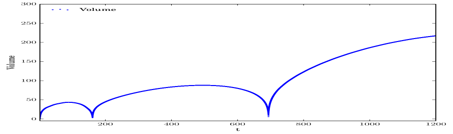
(a)

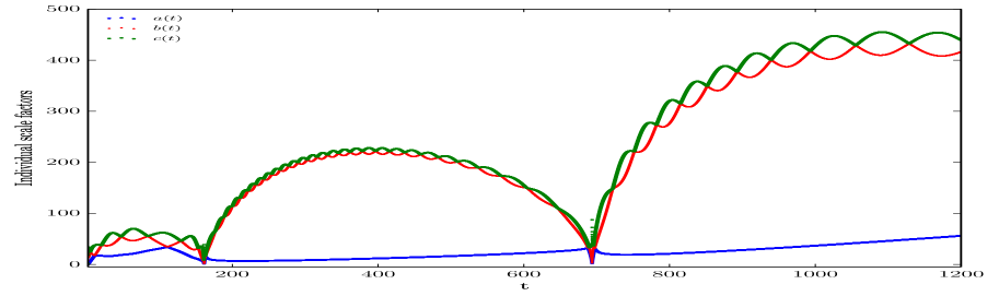
(b)

III.1 Effects of entropy increase

The effects of an increase in entropy from cycle to cycle of an isotropic oscillating closed universe were first considered by Tolman tol . He showed that there would be an increase in expansion volume maxima and cycle length from cycle to cycle as a consequence of the second law of thermodynamics. The total energy of the universe is zero in each cycle and successive oscillations drive the universe closer and closer to flatness.

If the dynamics are allowed to be anisotropic then we showed that, with $\Lambda=0$, increasing entropy leads to the increase of volume maxima and cycle length in successive cycles but the anisotropy grows from cycle to cycle in a manner that displays sensitive dependence on ‘initial’ conditions. We investigated this development in the context of the Bianchi type IX universe with comoving fluid velocities– the most general closed spatially homogeneous universe containing an isotropic FLRW universe as a particular case me . The addition of $\Lambda>0$ eventually terminates these oscillations, as in the isotropically expanding case.

In this paper we add an extra generalisation – the addition of non-comoving velocities to the most general anisotropic closed universe evolution with entropy increase. According to (20), the entropy increase from cycle to cycle should lead to a new effect: the reduction of the velocity from cycle to cycle. However, it is important to keep in mind that the constant on the right hand side of the conservation equation resulting from (20), that is equation (22), does not remain constant from cycle to cycle. Close to isotropy, the energy density $\rho\sim L^{3}(abc)^{-4/3}$, and the entropy density $s\propto\rho^{3/4}$ for radiation. Increasing the entropy density from cycle to cycle, means that $L$ remains constant only per cycle but jumps to a higher value in the next cycle. Thus, the constraint equation (22) is valid in each cycle with the right hand side being equal to a new, larger constant in subsequent cycles if there is entropy increase. A way of modelling this problem is to ensure that the constraint is imposed simultaneously with the injection of entropy at each minima. Thus, if we increase the entropy, or in our case the energy density (as $s\propto\rho^{3/4}$) by a factor $\Delta$, then the normalised velocities $v_{i}=\rho^{1/4}u_{i}$ must be multiplied by a factor $\Delta^{-1/4}$ to keep the constraint equation (22) unchanged. Thus we see that when the entropy increases, the velocities decrease as the evolution proceeds from cycle to cycle in accord with the second law of thermodynamics.

Figure 2: Evolution of the squares of velocities of non-comoving radiation with the increase in entropy with time $t$ in a Bianchi IX universe containing non-comoving radiation, as well as comoving dust and the ghost fields, the latter to facilitate the bounce. The velocity constraint (22) has been imposed. An increase in entropy(energy density) causes a decrease in the velocities and vice versa. Where necessary in the last two figures, the figure has been magnified to capture the rapidly oscillating features of the plot. From left, clockwise, the entropy density ($s\propto\rho^{3/4}$),the square of the spatial components of the velocities, $u_{1}^{2},u_{3}^{2}$ and $u_{2}^{2}$ are shown.

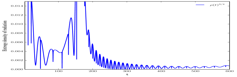
(a)

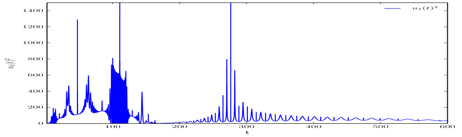
(b)

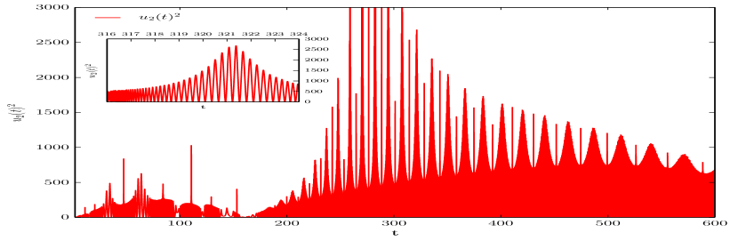
(c)

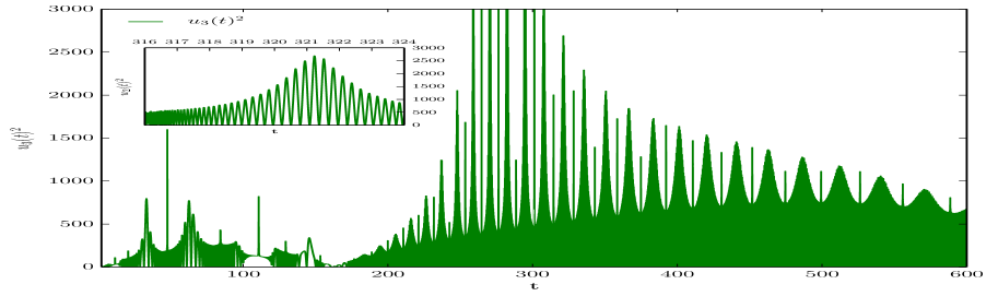
(d)

The sum of the square of the normalised velocities, $(\rho+p)^{1/4}u_{\alpha}$, oscillates initially but eventually settles down to a nearly constant value with small oscillations around this value even as oscillations proceed to higher and higher expansion maxima. In Figure 3, we show the constancy of this sum over one cycle. We have modelled the effects of radiation entropy, $s$, increase during a cycle of a closed universe by creating a sudden entropy increase at the start of each cycle. This produces the increase in the expansion maximum of successive cycles, first discovered by Tolman tol

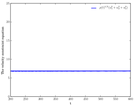
Figure 3: The evolution of (22), the velocity constraint equation, over one cycle

We identify a new feature of isotropic, oscillating radiation universes: any non-comoving velocities and vorticities will diminish from cycle to cycle as the expansion maxima increase and flatness is approached in accord with the second law of thermodynamics. For the anisotropic case, the overall trend in velocity evolution is oscillatory and is made more complicated. This is because we have shown that flatness is approached with an increase in expansion maxima and the inclusion of non-comoving velocities changes the dependence of the energy density and hence of the entropy on the scale factors from the isotropic case (and the anisotropic case in the absence of these non-comoving velocities) me . Thus we can only observe a increase/decrease in the velocities with a corresponding decrease/increase in the entropy. Aside from this effect, the evolutionary impact of the non-comoving velocities on the evolution in a cyclic radiation universe found in case with comoving velocities is only asymptotically logarithmic in time me .

Figure 4: Evolution of (a) the $3$-curvature and (b) the shear with the increase of entropy with time $t$ in a Bianchi IX universe where the radiation is not comoving with the tetrad frame, also containing a comoving dust field and a comoving ghost field to facilitate the bounce.

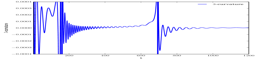
(a)

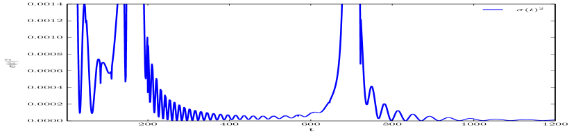
(b)

III.2 Evolution with non-comoving velocities

To study the behaviour of this model under the influence of non-comoving matter we assume that only the radiation field possesses non-comoving velocities (i.e. the ghost field is comoving). In the case of Bianchi IX, we find that the scale factors do undergo a bouncing behaviour, see Figure 1, as in the case without the non-comoving velocities. The volume scale factor, $abc$, mimics the behaviour of cube of the scale factor in the isotropic Friedmann case and shows an increase in height of its expansion maxima as the entropy of the constituents is increased from cycle to cycle. The individual scale factors oscillate out of phase with each other and with different expansion maxima, similar to their behaviour without the non-comoving velocities, see Figure 1. However, the period of the volume oscillations is greater than in the comoving velocities case. Thus, the model takes longer to recollapse on average than in the comoving case, making each cycle last longer in comoving proper $t$ time.  

Figure 5: (a), (b), and (c): Evolution of the squares of the 3-velocity components of non-comoving radiation with the increase in entropy in time $t$ in a Bianchi IX universe consisting of non-comoving radiation, as well as comoving dust and the ghost fields, the latter to facilitate the bounce. Unlike in Figures 2,2 and 2, the velocity constraint equation (22) has not been explicitly imposed. The evolution of $u_{2}(t)^{2}$ and $u_{3}(t)^{2}$ are highly oscillatory especially in the second cycle with very small time periods of oscillation, and to show this behaviour clearly, the plots are magnified and partly inset.

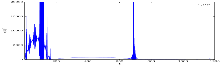
(a)

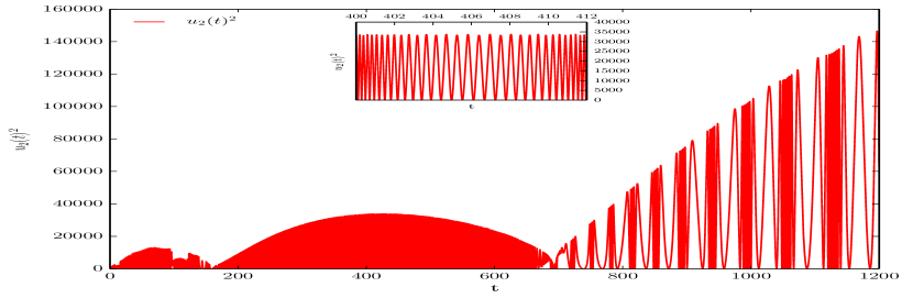
(b)

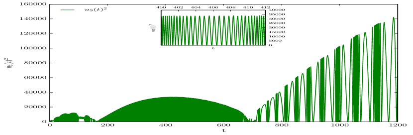
(c)

The shear and the $3$-curvature undergo oscillations which increase in amplitude and frequency near the minima and do not appear to fall to smaller and smaller values, see Figures 4 and 4.

The velocity components themselves show oscillatory behaviour, see Figures 5, 5 and 5. However, the amplitude of their oscillations undergoes cyclic behaviour. The amplitudes of oscillations fall to their smallest values at the expansion minima of the scale factors. After the first oscillation, one of the velocity components starts undergoing very small oscillations around a nearly constant value. We give an approximate analytic analysis of this evolution in the Appendix.

IV The effects of a cosmological constant

Figure 6: Evolution of (a) the shear, and (b) the $3$-curvature (left to right) and the individual scale factors with the increase in entropy with time $t$ in a Bianchi IX universe where the radiation is not comoving with the tetrad frame, containing a comoving dust field and a comoving ghost field to facilitate the bounce, together with a positive cosmological constant.

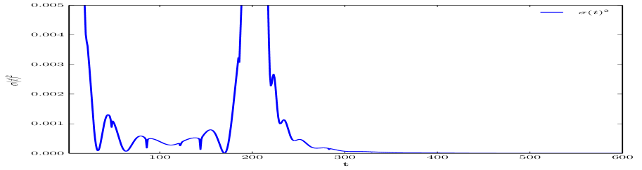
(a)

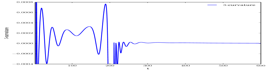
(b)

IV.1 Positive cosmological constant ($\Lambda>0$)

Now we add a cosmological constant to the model. The effect of cosmological constant domination in the case of comoving velocities was to cause the model to change from a cyclical behaviour to asymptotically de Sitter like expansion me (note that the cosmic no hair theorems nohair1 ; nohair2 do not cover the type IX case because the 3-curvature scalar can be positive).

Figure 7: Evolution of (a) the volume scale factor, and (b) the individual directional Hubble rates (left to right) with the increase in entropy, and a positive cosmological constant, with time $t$ in a Bianchi IX universe where the radiation is not comoving with the tetrad frame, also containing a comoving dust field and a comoving ghost field to facilitate the bounce. The blue starred, red dotted, and solid green lines correspond to derviatives of the principal values of the $3$-metric in the tetrad frame, Hubble rates $\dot{a}/a$, $\dot{b}/b$ and $\dot{c}/c$ respectively. The model undergoes approach to de Sitter expansion when the cosmological constant eventually dominates the dynamics after cycles become large enough to ensure this.

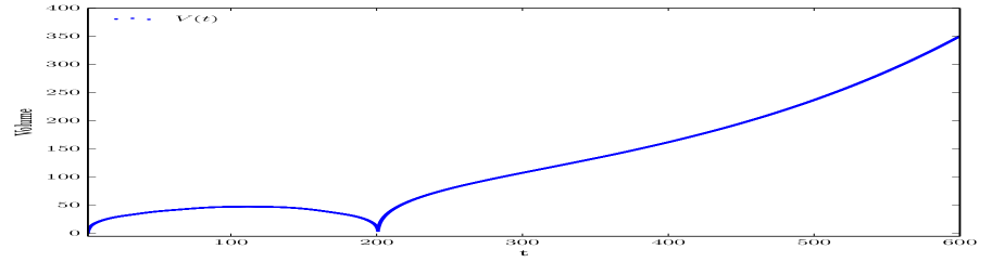
(a)

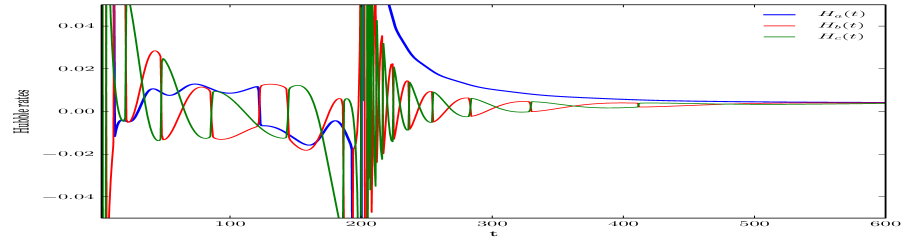
(b)

As in case with comoving velocities, the model is able to undergo cyclical behaviour until the maxima grow large enough for the cosmological constant to dominate at late times and then the dynamics approach a phase of quasi de Sitter expansion, see Figure 7. The individual expansion rates oscillate while the model is still undergoing cyclical behaviour but approach a constant value $H_{0}=\sqrt{\Lambda/3}$ signalling the onset of isotropic de Sitter behaviour, see Figure 7.

In the de Sitter phase the shear and the curvature are diluted by expansion, as expected, and fall exponentially rapidly to very small values, see Figures 6 and 6. The 3-curvature can be seen to change sign from negative values (when the dynamics are far from isotropy) to positive values (when the dynamics are close to isotropy). Positive 3-curvature is necessary for a volume maximum to occur.

Figure 8: Evolution of the squares of velocity components of non-comoving radiation with the increase in entropy with time $t$ in a Bianchi IX universe consisting of non-comoving radiation, as well as a comoving dust field and a comoving ghost field to facilitate the bounce, and a positive cosmological constant. The graphs (a), (b) and (c) plot the squares of the spatial components of the $4$-velocity in the tetrad frame, $u_{1}(t)^{2}$,$u_{2}(t)^{2}$, and $u_{3}(t)^{2}$, respectively.

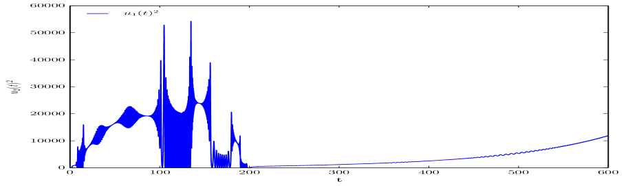
(a)

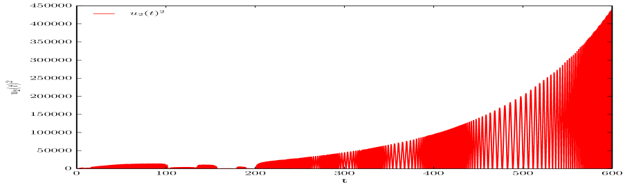
(b)

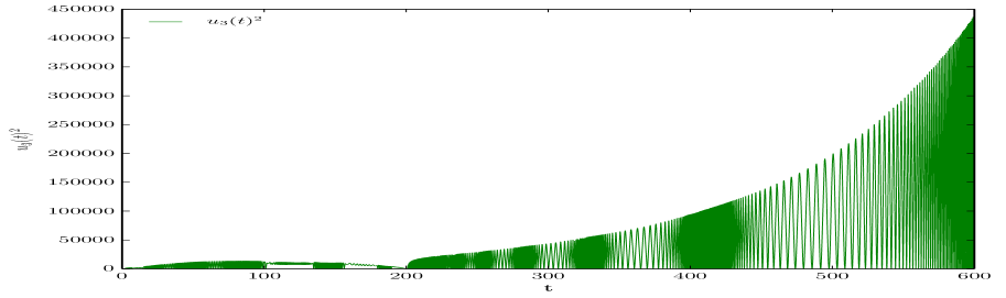
(c)

The velocities themselves oscillate rapidly in each cycle, while the amplitudes of the oscillations rise or fall according to the growth or regression of the scale factors, see Figures 8, 8 and 8. The amplitudes of the oscillations of the velocities in two of the directions grow with the exponential expansion of the scale factors. As the scale factors expand further, the time period of the oscillations of the velocities also increases.

IV.2 Negative cosmological constant ($\Lambda<0$)

Figure 9: Evolution of (a) the shear, and (b) the $3$-curvature with the increase of entropy with time $t$ in a Bianchi IX universe where the radiation is not comoving with the tetrad frame, as well as comoving dust and ghost field, the latter to facilitate the bounce, in the presence of a negative cosmological constant.

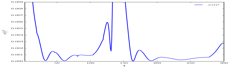
(a)

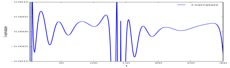
(b)

Adding a negative cosmological constant results in the universe always recollapsing tip , as this is just another null energy condition violating field. For the behaviour of the volume and individual scale factors, see Figures 10 and 10.

Figure 10: Evolution of (a) the volume scale factor and (b) the individual scale factors with $t$ in the presence of a negative cosmological constant in a Bianchi IX universe where the radiation is not comoving with the tetrad frame, and containing a comoving dust field and a comoving ghost field to facilitate the bounce. The blue starred, red dotted and green solid lines correspond to the principal values of the $3$-metric in the tetrad frame, scale factors $a(t)$, $b(t)$ and $c(t)$, respectively.

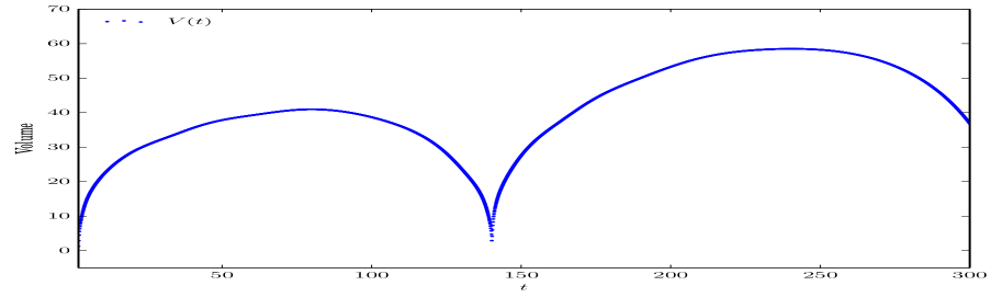
(a)

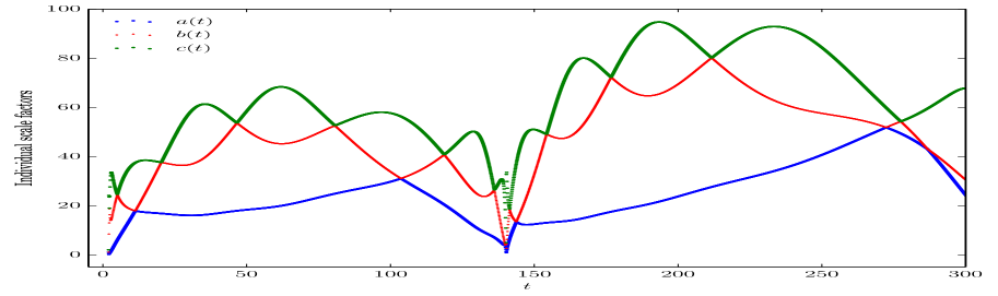
(b)

Figure 11: Evolution of the squares of the velocities of non-comoving radiation with time $t$ in a Bianchi IX universe consisting of non-comoving radiation, as well as comoving dust and ghost fields, the latter to facilitate the bounce, and a negative cosmological constant. Plots (a), (b) and (c) show the squares of the spatial components of the $4$-velocity in the tetrad frame, $u_{1}(t)^{2}$,$u_{2}(t)^{2}$, and $u_{3}(t)^{2}$, respectively. The highly oscillatory behaviour of the velocity components with very short time period is captured by the magnified insets in each of the plots.

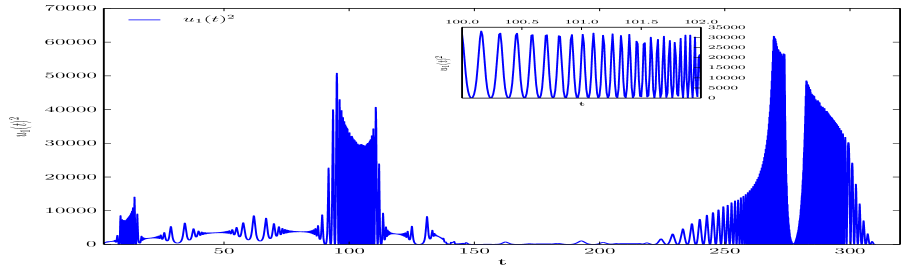
(a)

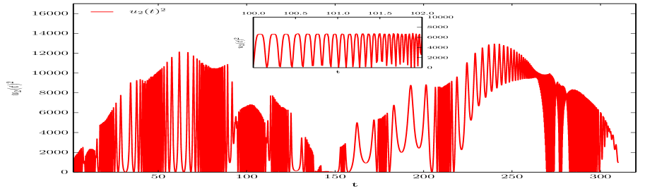
(b)

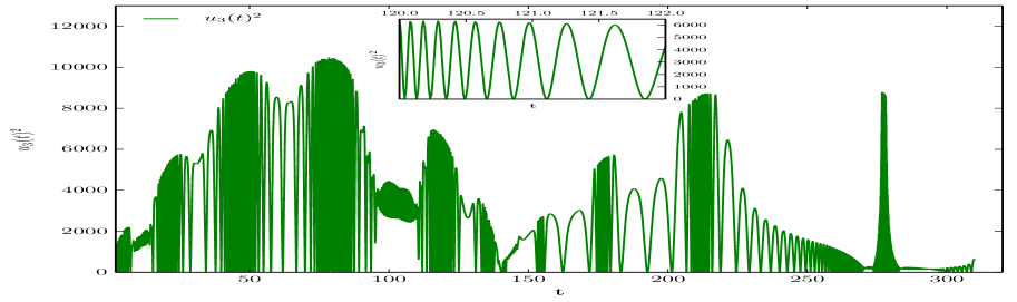
(c)

The ghost field allows the model to undergo more cycles of oscillation. As we are not introducing an increase in entropy and all the cycles are of equal size, we shall focus on one cycle. The velocities all oscillate and increase with the volume of the universe. One of the velocities ($u_{1}(t)^{2}$) also oscillates but with smaller amplitude around a constant value. Only at the end of each cycle does this velocity component show an increase in the amplitude of oscillations, see Figures 11, 11 and 11.

The shear and the $3$-curvature undergo oscillations, falling to their smallest values at the moments when the volume of the universe is at its highest, see Figures 9 and 9. Again, we see the 3-curvature taking on negative values when the dynamics are significantly anisotropic and positive values when close to isotropy.

V Conclusions

To complete the analysis of the shape of cyclic closed anisotropic universes, it is important to include the effects of non-comoving matter. In the current analysis, we have extended the results of me by including a radiation field that is not comoving with the reference tetrad frame. This tilted velocity field introduces vorticity, in addition to the shear and $3$-curvature anisotropies, into the universe.

We found that, as in the comoving case, the expansion maxima increases with increasing entropy of the constituents from cycle to cycle, while the individual scale factors oscillate out of phase with each other. The overall dynamics approach flatness over many cycles but they become increasingly anisotropic. We find a new effect in oscillating universes with non-comoving velocities and vorticity. Over successive cycles of entropy increase the conservation of momentum and angular momentum ensures that there is a decrease in the magnitude of the velocities and vorticities in response to the increase of entropy. We modelled entropy increase per cycle by adding entropy at the start of each cycle of a closed universe. We also included a comoving ghost field with negative energy density in order to create a bounce at finite expansion minima and avoid the chaotic mixmaster regime as $t\rightarrow 0$ – it is not relevant in practice to post-Planck time evolution.

Our numerical study shows that the velocities oscillate many times and around an almost constant value per cycle, and the amplitude of the oscillations increases with the increase in expansion volume. The velocity in one of the directions tends to a constant value after initially undergoing several oscillations. On explicitly imposing the constraint equation arising out of particle number conservation, see equation (22), we find that an increase in entropy density(and hence energy density as for radiation $s\propto\rho^{3/4}$) produces a corresponding decrease in the components of the non-comoving velocity, and vice versa.

When we add a positive cosmological constant to a model containing radiation and a ghost field we confirm that the oscillations are sustained until the cosmological constant dominates the dynamics, after which the scale factors enter a period of quasi de Sitter expansion. The velocities oscillate with amplitude increasing with increasing scale factor as before, but after cosmological constant domination, the time period of oscillations starts increasing, and they oscillate less rapidly, around a constant value. The asymptotic state is de Sitter with a constant velocity field.

When we add a negative cosmological constant we find there is always collapse, as expected. Studying one cycle we see that the scale factors oscillate out of phase with each other. The velocities in two directions oscillate with increasing amplitude as the volume increases but decrease again with decreasing volume. The velocity in the third direction, however, oscillates with very small amplitude around a constant value, only increasing in oscillation amplitude at the end of each cycle when the volume is its smallest.

We conclude that the inclusion of non-comoving velocities has the effect of increasing the time period of the oscillations of the model. The velocities oscillate rapidly per cycle but with increasing amplitude as the volume of the universe increases, in at least two directions. In the third direction, the velocity oscillates around a constant value with very small amplitude, and hence remains nearly constant per cycle. It only increases in amplitude when the model collapses, before relapsing again to a nearly constant value during the next cycle. Our analysis has identified the principal ingredients of a general cyclic closed universe in the case of spatial homogeneity. In a future work we will explore the effects of inhomogeneities on these conclusions.

Appendix A Approximate analysis of the radiation era

We seek an approximate solution of the velocity evolution equations in the type IX model during the radiation era. In our earlier study me without velocities we found a long period of evolution during the radiation era (before the curvature creates slow-down of the expansion near the volume maximum) with the scale factors evolving to a good approximation in a quasi-axisymmetric manner during the radiation era, as

$$a(t)=a_{0}t^{1/2}[\ln(t)]^{-1/2},b(t)=b_{0}t^{1/2}[\ln(t)]^{-1/2},c(t)=c_{0}t^{1/2}\ln(t).$$ (40)

When the effects of the velocities in the Bianchi type IX radiation universe are small they can be treated as test motions on an expanding radiation background governed by equations (20) and (21). We examine a typical case where we choose

$$v_{3}=\mathrm{constant.}$$

This is consistent with the velocity evolution equation for $v_{3}$ with $1/a^{2}=1/b^{2}.$In the approximation $a\gg b\gg c$ and $b^{4}>a^{2}c^{2}$ for large $t$ from ((34) and (35)), the evolution equations for $v_{1}$ and $v_{2}$ reduce to:

$$\dot{v}_{1}+\frac{v_{2}v_{3}}{v_{0}c^{2}}\left(1-\frac{2L^{3}}{w^{1/2}}\right)=0,$$

$$\dot{v}_{2}-\frac{v_{1}v_{3}}{v_{0}c^{2}}\left(1+\frac{2L^{3}b^{2}}{a^{2}w^{1/2}}\right)=0.$$

We assume non-relativistic velocities, so take $v_{0}=1$, and note that $w=\rho_{r}+p_{r}=4\rho_{r}/3$. Since $\rho_{r}\propto(abc)^{-4/3}\propto t^{-2}$, we write

$$w^{1/2}=\frac{M}{t},$$

where $M$ is a positive constant. Therefore the radiation entropy, $s$, depends on $M$ via

$$s\propto\rho_{r}^{3/4}\propto w^{3/4}\propto M^{3/2}.$$

Hence, we have approximately

$$\dot{v}_{1}+\frac{v_{2}v_{3}}{c_{0}^{2}t\ln^{2}(t)}\left(1-\frac{2L^{3}t}{M}\right)=0,$$ (41)

$$\dot{v}_{2}-\frac{v_{1}v_{3}}{c_{0}^{2}t\ln^{2}(t)}\left(1-\frac{2L^{3}b_{0}^{2}t\ }{Ma_{0}^{2}\ }\right)=0,$$ (42)

where $v_{3}$ is constant. At large times these equations are (and scaling $a_{0}=b_{0})$

$$\dot{v}_{1} = \frac{2L^{3}v_{3}v_{2}}{Mc_{0}^{2}\ln^{2}(t)}\equiv\frac{Dv_{2}}{\ln^{2}(t)},$$ (43)

$$\dot{v}_{2} = -\frac{2L^{3}v_{3}b_{0}^{2}v_{1}}{Mc_{0}^{2}a_{0}^{2}\ \ln^{2}(t)}\equiv-\frac{Dv_{2}}{\ln^{2}(t)},$$ (44)

where

$$D=\frac{2L^{3}v_{3}}{Mc_{0}^{2}}$$

is a constant. Hence,we see immediately that

$$v_{1}^{2}+v_{2}^{2}=E\mathrm{\ \ :}\text{ }E=\mathrm{\ constant.}$$ (45)

Since $v_{1}=\sqrt{E-v_{2}^{2},}$we have in (43)

$$\dot{v}_{1}=-v_{2}\dot{v}_{2}(E-v_{2}^{2})^{-1/2}=\frac{Dv_{2}}{\ln^{2}(t)},$$

hence

$$\int\frac{dv_{2}}{\sqrt{E-v_{2}^{2}}}=-D\int\frac{dt}{\ln^{2}(t)}$$

Therefore,

$$v_{2}=\sqrt{E}\sin\left(-D\int\frac{dt}{\ln^{2}(t)}\right),$$

and so, by (45), we have

$$v_{1}=\sqrt{E}\cos\left(-D\int\frac{dt}{\ln^{2}(t)}\right).$$

The components $v_{1}$ and $v_{2}$ therefore undergo bounded oscillations while $v_{3}$ remains constant.

We can get a better approx by keeping all the terms in (41) and (42). If we write them as

$$\dot{v}_{1}+\frac{Av_{2}\ }{t\ln^{2}(t)}\left(1-Bt\right)=0,$$ (46)

$$\dot{v}_{2}-\frac{Av_{1}\ }{t\ln^{2}(t)}\left(1-Bt\right)=0,$$ (47)

then $v_{1}^{2}+v_{2}^{2}=$ $E$, and hence we find a second order correction which confirms the oscillatory behaviour of he velocities with growing periods of oscillation:

$$v_{1} = E^{1/2}\cos\left(-\frac{1}{\ln(t)}-B\int\frac{dt}{\ln^{2}(t)}\right)$$

$$v_{2} = E^{1/2}\sin\left(-\frac{1}{\ln(t)}-B\int\frac{dt}{\ln^{2}(t)}\right)$$

- [1] Richard C Tolman. On the theoretical requirements for a periodic behaviour of the universe. Physical Review, 38(9):1758, 1931.
- [2] Iakov Borisovich Zeldovich and Igorʹ Dmitrievich Novikov. Relativistic astrophysics, 2: The structure and evolution of the Universe, volume 2. University of Chicago Press, 1971.
- [3] John D Barrow and Mariusz P Dabrowski. Oscillating universes. Monthly Notices of the Royal Astronomical Society, 275(3):850–862, 1995.
- [4] John D Barrow and Chandrima Ganguly. Cyclic mixmaster universes. Physical Review D, 95(8):083515, 2017.
- [5] Richard A Matzner, LC Shepley, and James B Warren. Dynamics of so (3, r)-homogeneous cosmologies. Annals of Physics, 57(2):401–460, 1970.
- [6] Andrew R King and George FR Ellis. Tilted homogeneous cosmological models. Communications in Mathematical Physics, 31(3):209–242, 1973.
- [7] VN Lukash. Homogeneous cosmological models with gravitational waves and rotation. JETP Letters, 19:265–267, 1974.
- [8] VN Lukash. Physical interpretation of homogeneous cosmological models. Il Nuovo Cimento B (1971-1996), 35(2):268–292, 1976.
- [9] VN Lukash, ID Novikov, and AA Starobinskii. Particle creation in the vortex cosmological model. Zhurnal Eksperimentalnoi i Teoreticheskoi Fiziki, 69:1484–1500, 1976.
- [10] VN Lukash, ID Novikov, AA Starobinsky, and Ya B Zeldovich. Quantum effects and evolution of cosmological models. Il Nuovo Cimento B (1971-1996), 35(2):293–307, 1976.
- [11] LP Grishchuk, AG Doroshkevich, and VN Lukash. The model of “mixmaster universe” with arbitrarily moving matter. Soviet Journal of Experimental and Theoretical Physics, 34:1, 1972.
- [12] John D Barrow and Christos G Tsagas. On the stability of static ghost cosmologies. Classical and Quantum Gravity, 26(19):195003, 2009.
- [13] John D Barrow, Dagny Kimberly, and Joao Magueijo. Bouncing universes with varying constants. Classical and Quantum Gravity, 21(18):4289, 2004.
- [14] Charles W Misner. Mixmaster universe. Physical Review Letters, 22(20):1071, 1969.
- [15] O Heckmann and E Schucking. Relativistic cosmology. Gravitation, an Introduction to Current Research, page 438, 1962.
- [16] David F. Chernoff and John D. Barrow. Chaos in the mixmaster universe. Phys. Rev. Lett., 50:134–137, Jan 1983.
- [17] Lev Davidovich Landau and Evgenii Mikhailovich Lifshitz. The classical theory of fields. 1971.
- [18] John D. Barrow and Mariusz P. Da¸browski. Kantowski-sachs string cosmologies. Phys. Rev. D, 55:630–638, Jan 1997.
- [19] AA Starobinskii. Isotropization of arbitrary cosmological expansion given an effective cosmological constant. JETP lett, 37(1), 1983.
- [20] Vladimir A Belinskii, Isaak M Khalatnikov, and Evgeny M Lifshitz. A general solution of the einstein equations with a time singularity. Advances in Physics, 31(6):639–667, 1982.
- [21] John D. Barrow. Chaos in the einstein equations. Phys. Rev. Lett., 46:963–966, Apr 1981.
- [22] AG Doroshkevich, VN Lukash, and ID Novikov. The isotropization of homogeneous cosmological models. Sov. Phys.–JETP, 37:739–46, 1973.
- [23] John D Barrow. On the origin of cosmic turbulence. Monthly Notices of the Royal Astronomical Society, 179(1):47P–49P, 1977.
- [24] Robert M. Wald. Asymptotic behavior of homogeneous cosmological models in the presence of a positive cosmological constant. Phys. Rev. D, 28:2118–2120, Oct 1983.
- [25] John D Barrow. The very early universe. In Proceedings of the Nuffield Workshop), ed. GW Gibbons, SW Hawking and STC Siklos, volume 267, 1983.
- [26] F.J. Tipler. Singularities in universes with negative cosmological constant. Astrophys. J. , 209:12–15, October 1976.