Evaluating the accuracy of the dynamic mode decomposition

Abstract

Dynamic mode decomposition (DMD) gives a practical means of extracting dynamic information from data, in the form of spatial modes and their associated frequencies and growth/decay rates. DMD can be considered as a numerical approximation to the Koopman operator, an infinite-dimensional linear operator defined for (nonlinear) dynamical systems. This work proposes a new criterion to estimate the accuracy of DMD on a mode-by-mode basis, by estimating how closely each individual DMD eigenfunction approximates the corresponding Koopman eigenfunction. This approach does not require any prior knowledge of the system dynamics or the true Koopman spectral decomposition. The method may be applied to extensions of DMD (i.e., extended/kernel DMD), which are applicable to a wider range of problems. The accuracy criterion is first validated against the true error with a synthetic system for which the true Koopman spectral decomposition is known. We next demonstrate how this proposed accuracy criterion can be used to assess the performance of various choices of kernel when using the kernel method for extended DMD. Finally, we show that our proposed method successfully identifies modes of high accuracy when applying DMD to data from experiments in fluids, in particular particle image velocimetry of a cylinder wake and a canonical separated boundary layer.

1 Introduction

The decomposition of spatiotemporal data into spatial modes and temporal functions describing their evolution gives a means to isolate coherent features and assemble low-order representations of complex dynamics. Over the past decade, the dynamic mode decomposition (DMD) [22] has become a routinely-used method for such purposes [21, 25, 6, 30]. See, for example, [17] and [20] for reviews of many ensuing uses and applications of DMD. While successfully used on a range of datasets, general questions still exist in terms of how to select a reduced set of modes, and how to ensure results are quantitatively accurate. On the first point, numerous methods have been proposed to select a reduced number of modes that best represent the dynamics of the system [3, 29, 15, 16]. On the second point, the sensitivity of the outputs of DMD to noisy data has also been investigated [7, 1], and a number of modified algorithms proposed that give improved accuracy for noisy data [13, 5].

The present work differs from these past studies by giving a means of estimating the accuracy of DMD on a mode-by-mode basis, without any a-priori knowledge of the system dynamics, noise characteristics, or truncation of low-energy modes. It has been shown previously [21, 26] that DMD approximates the Koopman operator, an infinite-dimensional linear operator defined for (nonlinear) dynamical systems. In this work, we will exploit this connection by estimating the accuracy to which we approximate eigenfunctions of the Koopman operator. This approach allows our analysis to naturally extend to extensions of DMD [27] that are designed to improve the approximation to the Koopman operator for nonlinear systems. Extended DMD uses nonlinear observables to expand the space in which the Koopman operator is approximated. However, EDMD suffers from the curse of dimensionality: that is, the computational cost increases rapidly with the dimension of the state. To circumvent this issue, kernel DMD (KDMD) [28] was proposed as a computationally inexpensive alternative, which makes use of a kernel function to implicitly include a rich (and nonlinear) set of observables, while maintaining the same computational cost as DMD. The optimal choice of kernel function for KDMD is still an open question, and here we demonstrate that the accuracy criterion may be used to evaluate and compare the performance of various kernels.

The structure of this work is as follows. We first review DMD, the Koopman operator, and kernel DMD in section 2, before presenting and validating our proposed accuracy criterion in section 3. Section 4 uses the accuracy criterion to measure the performance of various kernels in KDMD for a simple nonlinear system, while section 5 demonstrates that this criterion is effective in selecting accurate DMD modes from experimental data.

2 Background

We first give a review of previous results, including the DMD algorithm and its connections to the Koopman operator (section 2.1), as well as extensions of DMD that can better approximate the Koopman operator for nonlinear systems (section 2.2).

2.1 Dynamic mode decomposition

Dynamic mode decomposition was introduced in [22], and our presentation here follows that in [26, 20]. Consider a discrete-time dynamical system whose state space is denoted by $X\subset\mathbb{R}^{n}$, and suppose the dynamics are given by

$$\bm{x}({k+1})=\bm{F}(\bm{x}({k})),\quad\bm{x}(k)\in X.$$ (2.1)

Let $\psi_{1},\ldots,\psi_{q}$ be real-valued functions on $X$, which we call observables, and let $\bm{\psi}\mathrel{\mathop{\ordinarycolon}}X\to\mathbb{R}^{q}$ denote the vector-valued function whose components are $(\psi_{1},\ldots,\psi_{q})$. We may not be able to measure the state $\bm{x}$ directly, but instead, we can measure the vector

$$\bm{y}=\bm{\psi}(\bm{x}).$$

As a special case, $\bm{y}$ could be the state itself, i.e., $\bm{y}=\bm{\psi}(\bm{x})=\bm{x}$. For complex systems, it can be advantageous to define observables that are nonlinear functions of the state, which will be discussed in more detail in section 2.2. For the purposes of describing standard DMD, we assume $\bm{y}=\bm{x}$.

We consider pairs of snapshots $(\bm{x}_{k},\bm{x}^{\#}_{k})$, with $\bm{x}_{k}\in X,k=1,2,\cdots,m$, and where $\bm{x}^{\#}_{k}=F(\bm{x}_{k})$ is the image of $\bm{x}_{k}$ upon application of the dynamics (2.1). For sequential data, $\bm{x}(1),\ldots,\bm{x}(m+1)$ satisfying (2.1), one takes $\bm{x}_{k}=\bm{x}(k)$, $\bm{x}^{\#}_{k}=\bm{x}({k+1})$, though non-sequential data may also be used, such as from multiple runs of experiments or simulations [26]. In DMD, we seek a matrix $\bm{A}\in\mathbb{R}^{q\times q}$ such that

$$\bm{y}^{\#}_{k}=\bm{A}\bm{y}_{k},\ \ k=1,2,\cdots,m$$

holds, at least approximately. We form two matrices

$$\bm{Y}=\begin{bmatrix}\bm{y}_{1}&\bm{y}_{2}&\cdots&\bm{y}_{m}\end{bmatrix},\quad\bm{Y}^{\#}=\begin{bmatrix}\bm{y}^{\#}_{1}&\bm{y}^{\#}_{2}&\cdots&\bm{y}^{\#}_{m}\end{bmatrix},$$

and define the DMD matrix $\bm{A}$ by

$$\bm{A}=\bm{Y}^{\#}\bm{Y}^{+}.$$ (2.2)

DMD modes and eigenvalues are the eigenvectors and eigenvalues of $\bm{A}$. A typical algorithm to compute these modes and eigenvalues is as follows[26]:

Algorithm (DMD)

1. Compute the reduced SVD $\bm{Y}=\bm{U}\bm{\Sigma}\bm{V}^{T}$.

2. (Optional) Truncate the SVD by only retaining the first $r$ colunms of $\bm{U},\bm{V}$, and the first $r$ rows and columns of $\bm{\Sigma}$, to obtain $\bm{U}_{r},\bm{\Sigma}_{r},\bm{V}_{r}$.

3. Let $\tilde{\bm{A}}=\bm{U}_{r}^{T}\bm{A}\bm{U}_{r}=\bm{U}_{r}^{T}\bm{Y}^{\#}\bm{V}_{r}\bm{\Sigma}_{r}^{-1}$, $\tilde{\bm{A}}\in\mathbb{R}^{r\times r}$.

4. Find the eigenvalues $\mu_{i}$ and eigenvectors $\tilde{\bm{v}}_{i}$ of $\tilde{\bm{A}}$, such that $\tilde{\bm{A}}\tilde{\bm{v}}_{i}=\mu_{i}\tilde{\bm{v}}_{i}$.

5. The (projected) DMD modes are given by $\bm{v}_{i}=\bm{U}_{r}^{T}\tilde{\bm{v}}_{i}$, with corresponding (discrete-time) DMD eigenvalues $\mu_{i}$.

The eigenvectors of the matrix $\bm{A}\in\mathbb{R}^{q\times q}$ can be found from the eigenvectors of the smaller matrix $\tilde{\bm{A}}\in\mathbb{R}^{r\times r}$. We denote the eigenvalues and eigenvectors of $\bm{A}$ by $\{\mu_{i},\bm{v}_{i}\}$. In the case of sequential data (for which $\bm{y}^{\#}_{k}=\bm{y}_{k+1}$), suppose that we can express the initial state as

$$\bm{y}_{1}=\sum_{i=1}^{q}c_{i}\bm{v}_{i}.$$

The time evolution of the system (starting at $\bm{y}_{1}$) is then predicted by DMD to be

$$\bm{y}_{k+1}=\bm{A}^{k}\bm{y}_{1}=\sum_{i=1}^{q}c_{i}\mu_{i}^{k}\bm{v}_{i}.$$ (2.3)

Therefore, each DMD mode $\bm{v}_{i}$ is associated with a single frequency and growth/decay rate (DMD eigenvalue $\mu_{i}$). In reality, (2.3) may not hold exactly, depending on the quantity and quality of data used, whether the system dynamics are nonlinear, whether the SVD is truncated in step 2 of the DMD algorithm above. For cases where equation (2.3) does not give an exact description of the dynamics, DMD gives a least-squares fit to the data (as pairs of snapshots).

There are connections between DMD and an infinite-dimensional linear operator called the Koopman operator [26, 21], with the high-level idea being that DMD gives a finite-dimensional numerical approximation of the Koopman operator. Our proposed criterion for evaluating the accuracy of DMD exploits this connection. For a given state-space $X$, the Koopman operator acts on scalar-valued functions of $X$, which we referred earlier as observables. Here, we consider observables in $L^{2}(X)$, the space of square integrable functions on $X$. Given the dynamics in (2.1), one then defines the Koopman operator $\mathcal{K}\mathrel{\mathop{\ordinarycolon}}L^{2}(X)\to L^{2}(X)$ by

$$(\mathcal{K}\phi)(\bm{x})=(\phi\circ\bm{F})(\bm{x})=\phi(\bm{F}(\bm{x})).$$ (2.4)

That is, $\mathcal{K}$ maps a function $\phi$ to another function $\phi\circ\bm{F}$, and $(\mathcal{K}\phi)(\bm{x})$ gives the value of $\phi(\bm{x})$ at the next time step. Here we emphasize two points: first that the Koopman operator acts on functions of the state instead of the state itself; and second that the Koopman operator is linear, even though the dynamics might be nonlinear. On the second point, note that

$$\mathcal{K}(c_{1}\phi_{1}+c_{2}\phi_{2})=c_{1}\mathcal{K}\phi_{1}+c_{2}\mathcal{K}\phi_{2}$$

holds for any functions $\phi_{1},\phi_{2}$ and any scalars $c_{1},c_{2}$. Since the Koopman operator is linear, it may have eigenvalues and eigenfunctions, which satisfy

$$\mathcal{K}\varphi=\mu\varphi,$$ (2.5)

where $\varphi$ is the eigenfunction with eigenvalue $\mu$.

Now, suppose we have a given set of observables $\{\psi_{1},\psi_{2},\cdots,\psi_{q}\}$, and suppose $\varphi$ is a Koopman eigenfuntion (with eigenvalue $\mu$) that lies in the span of $\{\psi_{j}\}$: i.e.,

$$\varphi(\bm{x})=\bar{w}_{1}\psi_{1}(\bm{x})+\cdots+\bar{w}_{q}\psi_{q}(\bm{x})=\bm{w}^{*}\bm{\psi}(\bm{x}),$$ (2.6)

for some $\bm{w}^{*}\in\mathbb{C}^{n}$. Then one can show (see [26, §4.1]) that under certain conditions on the data, $\bm{w}^{*}$ is a left eigenvector of the DMD matrix $\bm{A}$ with eigenvalue $\mu$ (i.e., $\bm{w}^{*}\bm{A}=\mu\bm{w}^{*}$). This connection implies that we can approximate Koopman eigenfunctions (and eigenvalues) for a given unknown dynamical system directly from data using DMD. In particular, given left eigenvectors of the DMD matrix ($\bm{w}_{i}^{*}\bm{A}=\mu_{i}\bm{w}_{i}^{*}$), we consider $\varphi_{i}(\bm{x})=\bm{w}_{i}^{*}\bm{\psi}(\bm{x})$ as a DMD-approximated Koopman eigenfunction, with eigenvalue $\mu_{i}$.

2.2 Extended DMD and kernel DMD

In order to apply the connection between DMD and Koopman mentioned above, the Koopman eigenfunctions must lie within the space spanned by the observables $\{\psi_{j}\}$. If one takes $\bm{\psi}(\bm{x})=\bm{x}$, as with standard DMD, then the subspace spanned by $\{\psi_{j}\}$ consists only of linear functions of $\bm{x}$, and this subspace is often not large enough to include eigenfunctions of $\mathcal{K}$ (a notable exception being the case in which $\bm{F}$ is linear). Extended DMD (EDMD) was proposed in [27] in order to enlarge the subspace of observables, and therefore better approximate Koopman eigenfunctions. In particular, Extended DMD approximates the Koopman operator by a weighted residual method, with trial functions given by $\{\psi_{j}\}$ and a particular choice of test functions specified by the data. Examples of observables $\psi_{j}(\bm{x})$ could include polynomials, Fourier modes, indicator functions, or spectral elements, as suggested in [27]. For instance, if we take $\bm{x}\in\mathbb{R}^{2}$ and take observables to be monomials in components of $\bm{x}$ up to degree $d=2$ (including the constant 1), then the vector of observables is

$$\bm{\psi}(\bm{x})=\begin{bmatrix}1&x_{1}&x_{2}&x_{1}^{2}&x_{1}x_{2}&x_{2}^{2}\end{bmatrix}^{T}.$$

We can potentially approximate many more accurate Koopman eigenfunctions with EDMD than we could with DMD. However, EDMD suffers from the curse of dimensionality [2]. If the state dimension is $n$ and we consider (multivariate) polynomials up to degree $d$, then the number of observables is $q=\binom{n+d}{d}$, which is approximately $n^{d}$ for large $n$. For large problems (as arise in fluids), data might typically have $n\approx 10^{6}$, so even if one considers only quadratic polynomials, the number of observables is $q\approx 10^{12}$, too large for practical computation. It is thus very computationally expensive to consider large subspaces of observables.

Kernel DMD (KDMD) has been proposed to deal with this curse of dimensionality [28]. In KDMD, EDMD is reformulated such that only inner products of observables need to be computed. The inner product can be evaluated by making use of a kernel function, a common technique in the community of machine learning. A kernel function $k\mathrel{\mathop{\ordinarycolon}}\mathbb{R}^{n}\times\mathbb{R}^{n}\rightarrow\mathbb{R}$ is defined as

$$k(\bm{x},\hat{\bm{x}})=\langle\bm{\psi}(\bm{x}),\bm{\psi}(\hat{\bm{x}})\rangle.$$ (2.7)

To appreciate how kernel functions work, consider for example a polynomial kernel $k(\bm{x},\hat{\bm{x}})=(1+\bm{x}^{T}\hat{\bm{x}})^{d}$ as an example. This kernel corresponds to a set of observables $\bm{\psi}(\bm{x})$ consisting of all monomials in components of $\bm{x}$ up to degree $d$ [2]. Taking $n=2$ and $d=2$, this kernel function can be expanded as

$$(1+\bm{x}^{T}\hat{\bm{x}})^{2} =1+2x_{1}\hat{x}_{1}+2x_{2}\hat{x}_{2}+2x_{1}^{2}\hat{x}_{1}^{2}+2x_{1}x_{2}\hat{x}_{1}\hat{x}_{2}+\hat{x}_{1}^{2}\hat{x}_{2}^{2}$$ (2.8)

$$=\langle\bm{\psi}(\bm{x}),\bm{\psi}(\hat{\bm{x}})\rangle,$$

where $\bm{\psi}(\bm{x})=(1,\sqrt{2}x_{1},\sqrt{2}x_{2},x_{1}^{2},\sqrt{2}x_{1}x_{2},x_{2}^{2})$. In the terminology of machine learning, $\bm{\psi}$ is called the feature map, and $\bm{\psi}(\bm{x})\in\mathbb{R}^{q}$ is called the feature space (which might be infinite dimensional). In the example above, the dimension of the (implicitly defined) feature space is $q=6$, but in order to compute $k(\bm{x},\hat{\bm{x}})$, we require inner products only in state space, which has dimension $n=2$. Kernel functions hence can be used to evaluate the inner product in a high dimensional (or even infinite dimensional) feature space in an efficient way. More examples of kernel functions are given in section 4.1.

3 Accuracy criterion for DMD

The connection between DMD and the Koopman operator as discussed in section 2.1 implies that we can use variants of DMD (e.g., DMD, EDMD, or KDMD) to approximate Koopman eigenfunctions and eigenvalues, given access to data. By applying DMD variants to a given dataset, we can potentially identify many Koopman eigenfunctions and eigenvalues (which we refer to as eigenpairs). However, the reliability of these eigenpairs remains unknown. Before using DMD results for any analysis or reduced order modeling, it is desirable and necessary to assess the quality (i.e., accuracy) of the results. In this section, we will develop a criterion for evaluating the accuracy of DMD-approximated Koopman eigenpairs. We describe this accuracy criterion in section 3.1, and then validate it in section 3.2 using a simple nonlinear system where the analytical Koopman eigenpairs are known.

The most common way to select which of the computed DMD modes are most relevant is to use the “mode amplitude”: for sequential data, one projects the initial condition onto DMD modes and one views the magnitude of the projection coefficients as the mode amplitudes. It is common practice [26, 12, 21] to retain the modes of largest amplitude. This approach sounds plausible; however, it was observed in [15] (which used sparsity-promoting techniques to select modes) that mode amplitude is not always a useful criterion for mode selection. Indeed, mode amplitudes can be misleading, as we illustrate below with a simple example.

Suppose we have three DMD modes,

$$\bm{v}_{1}=(1,0,0),\qquad\bm{v}_{2}=(0,1,0),\qquad\bm{v}_{3}=(0,1,\epsilon),$$ (3.1)

where $\epsilon$ is small and thus $\bm{v}_{2}$ and $\bm{v}_{3}$ are almost parallel. If we consider an initial condition $\bm{x}_{0}=(1,0,\zeta)$, and project it onto these DMD modes, we obtain

$$\bm{x}_{0}=\bm{v}_{1}-\frac{\zeta}{\epsilon}\bm{v}_{2}+\frac{\zeta}{\epsilon}\bm{v}_{3}.$$ (3.2)

For instance, if $\zeta=10^{-3}$ and $\epsilon=10^{-6}$, then $\zeta/\epsilon=10^{3}$, so the mode amplitude (defined as the magnitude of the projection coefficients) indicates that $\bm{v}_{2}$ and $\bm{v}_{3}$ are much more important than $\bm{v}_{1}$. The mode amplitudes indicate that we might be able to neglect $\bm{v}_{1}$ without significant adverse effects. However, it is clear that $\bm{v}_{1}$ is much more relevant for reconstructing $\bm{x}_{0}$: if we use only $\bm{v}_{2}$ and $\bm{v}_{3}$, we obtain

$$-\frac{\zeta}{\epsilon}\bm{v}_{2}+\frac{\zeta}{\epsilon}\bm{v}_{3}=(0,0,\zeta),$$ (3.3)

which does not accurately approximate $\bm{x}_{0}=(1,0,\zeta)$. A better approximation to $\bm{x}_{0}$ is simply $\bm{v}_{1}=(1,0,0)$. This example illustrates that mode amplitude is not always a reliable criterion for selecting which modes are important, especially when modes are almost parallel. Note that this problem would also arise if using other methods to measure mode amplitude (e.g., [16]).

The accuracy criterion we describe below does not provide a way of selecting which modes are dominant, and in the example above, accuracy of the modes did not play a role. However, the accuracy criterion can provide a way of eliminating candidate modes that we know to be inaccurate, so in this way it can help with the problem of mode selection.

3.1 Proposed accuracy criterion

Given data from an experiment or simulation, we can split the dataset into training data and testing data. Training data is used to approximate DMD modes (and associated Koopman eigenpairs), while testing data is used to evaluate the quality of these identified modes. Data-driven algorithms may suffer from the problem of over-fitting [11], so any evaluation criteria should use testing data that differs from the training data.

The idea of our approach is to evaluate the accuracy of a DMD mode (and eigenvalue) by looking at the accuracy of its corresponding Koopman eigenfunction. Suppose we are given an approximate Koopman eigenpair $(\mu,\varphi)$, and we wish to evaluate its accuracy. If $(\mu,\varphi)$ were a true Koopman eigenpair, then by definition it would satisfy

$$\varphi\circ\bm{F}=\mu\varphi,$$

where $\bm{F}$ defines the dynamics in (2.1). Ideally, we would like to compute

$$\frac{\|\varphi\circ\bm{F}-\mu\varphi\|}{\|\varphi\|},$$ (3.4)

where $\|\cdot\|$ is the norm of a function. (We divide by $\|\varphi\|$ so that the above quantity is independent of the scaling of the eigenfunction $\|\varphi\|$.) However, in order to compute (3.4), we require explicit knowledge of the dynamics $\bm{F}$, which is unknown in most cases of interest. Instead, we can estimate the above quantity using finite number of data points (i.e., the testing data). The estimation should give some sense of the quantity in (3.4), using only the testing data, which consists of pairs of samples $(\bm{x}_{k},\bm{x}_{k}^{\#})$ with $\bm{x}_{k}\in X$ and $\bm{x}_{k}^{\#}=\bm{F}(\bm{x}_{k})$. This observation motivates the following definition of an accuracy criterion:

$$\alpha=\frac{\sum_{k}|\varphi(\bm{x}_{k}^{\#})-\mu\varphi(\bm{x}_{k})|}{\sum_{k}|\varphi(\bm{x}_{k})|},$$ (3.5)

where $|\cdot|$ denotes the absolute value, and the summation is over the entire testing dataset. A diagram summarizing how this accuracy criterion may be applied is shown in Figure 1. More specifically, given a DMD-approximated eigenfunction $\varphi(\bm{x})=\bm{w}^{*}\bm{\psi}(\bm{x})$ with eigenvalue $\mu$ (i.e., $\bm{w}^{*}\bm{A}=\mu\bm{w}^{*}$, with $\bm{A}$ as defined in (2.2)), the accuracy criterion, or estimated mode error, can be written as

$$\alpha=\frac{\sum_{k}|\bm{w}^{*}\bm{\psi}(\bm{x}_{k}^{\#})-\mu\bm{w}^{*}\bm{\psi}(\bm{x}_{k})|}{\sum_{k}|\bm{w}^{*}\bm{\psi}(\bm{x}_{k})|}.$$ (3.6)

Figure 1: A diagram summarizing the implementation of the accuracy criterion. Training data is used to approximate Koopman eigenpairs with variants of DMD, while testing data is used to evaluate the quality of Koopman eigenpairs.

The numerator measures to what extent the eigenfunction equation holds, and the denominator gives a measure of the magnitude of the eigenfunction. Here $\alpha$ can be interpreted as the error of a Koopman eigenpair. The error is defined on a mode-by-mode basis, which enables independent evaluation for each individual DMD mode. Therefore it makes sense to call $\alpha$ the mode error. Observe that $\alpha$ is always non-negative, and it is usually less than 1. When we feed in the true Koopman eigenfunction and eigenvalue into $\alpha$ in equation (3.5), then $\alpha=0$ (assuming that the testing data is noise-free). If $\alpha$ is close to 1, the Koopman eigenpair is extremely unreliable, because the discrepancy in the eigenfunction equation is of the same order as the magnitude of the eigenfunction. Therefore, usually we only care about the DMD eigenpairs for which $0\leq\alpha\ll 1$. In our definition in (3.5), we have used the absolute value to indicate the discrepancy in the eigenfunction equation. However, it is also possible to use other norms, such as the $\ell^{2}$ norm (or its square), which yield similar results in terms of indicating relative accuracy of modes.

A meaningful evaluation criterion should be (fairly) independent the scaling of the eigenfunctions, the scaling of the testing data, and the size of the testing set. The proposed accuracy criterion approximately satisfies all of these. To show this, we consider the simple case where the full system state is used in DMD, i.e., $\bm{\psi}(\bm{x})=\bm{x}$ and the DMD-computed eigenfunction is linear, i.e., $\varphi(\bm{x})=\bm{w}^{*}\bm{\psi}(\bm{x})=\bm{w}^{*}\bm{x}$. The fact that we normalize by the magnitude of the observables means that $\alpha$ is relatively independent of eigenfunction scaling, data scaling, and data quantity, as is desired. In the case where the observable is not the full state (i.e., when using EDMD or KDMD), the scaling of the eigenfunctions and size of testing again do not influence $\alpha$, for the same reason. However, due to the nonlinear transformation $\bm{\psi}(\bm{x})$, the scaling of testing data $\bm{x}$ may play some role in the size of $\alpha$. Fortunately, it is reasonable to expect that the relative magnitude of $\alpha$ should still indicate the relative accuracy of different DMD-computed Koopman eigenpairs.

We point out that if the testing data is clean, mode error is determined only by the quality of DMD-approximated Koopman eigenpairs. If the testing data is noisy, mode error is also affected by the noise in testing data. For experimental data, we have access only to the noisy measurements. In these cases, the relative magnitude of $\alpha$ is still expected to indicate relative accuracy of Koopman eigenpairs. We reiterate again that this definition of error does not assume access to analytical Koopman spectral decomposition, which is unknown in most cases.

3.2 Validating the accuracy criterion

We have proposed an accuracy criterion that exploits the connection between DMD and the Koopman operator. Before applying this criterion to real data, we first seek to validate it as a reliable measure of accuracy. We will first consider a simple 2D nonlinear system for which the analytical Koopman spectral decomposition is known. Given analytical Koopman eigenpairs, we can define the true error to be the distance between the DMD eigenvalue and the true eigenvalue (eigenvalue error), or the difference between the DMD eigenfunction and the true eigenfunction (eigenfunction error). We will validate the accuracy criterion against the true error, and show that accuracy criterion reliably indicates accuracy.

Here we consider a 2D nonlinear map (also considered in [26]) with dynamics defined by

$$\begin{bmatrix}x_{1}\\ x_{2}\end{bmatrix}\mapsto\begin{bmatrix}\gamma x_{1}\\ \delta x_{2}+(\gamma^{2}-\delta)x_{1}^{2}\end{bmatrix},\quad\gamma=0.9,\delta=0.8.$$ (3.7)

It is straightforward to verify that $\gamma,\delta$ are Koopman eigenvalues with respective eigenfunctions

$$\varphi_{\gamma}(\bm{x})=x_{1},\qquad\varphi_{\delta}(\bm{x})=x_{2}-x_{1}^{2}.$$

Additional Koopman eigenvalues and eigenfunctions are given by

$${\mu}_{k,\ell}=\gamma^{k}\delta^{\ell},\qquad{\varphi}_{k,\ell}=\varphi^{k}_{\gamma}\varphi^{\ell}_{\delta},$$ (3.8)

where $k,\ell=0,1,2,\cdots$ are non-negative integers. Notice that the analytical eigenfunctions are multivariate polynomials in the state variables.

To collect training data, $m=100$ random initial points are sampled from a uniform distribution on $[-1,1]\times[-1,1]$, and their images are found by applying the map defined in equation (3.7). Similarly we also generate $m_{\text{test}}=100$ snapshot pairs as the testing data. The generated training and testing dataset are used for subsequent analysis in both this and the next section.

Here we apply EDMD with monomials as observables. In particular, the observables are taken to be

$$\psi_{k,\ell}(\bm{x})=x_{1}^{k}x_{2}^{\ell},\quad k,\ell=0,1,2,3,4,5,$$

where the feature space dimension is $q=6\times 6=36$. The results of applying EDMD are shown in Figure 2(a). We note that mode error indicates that leading eigenvalues are approximated very accurately ($\alpha\sim 10^{-15}$), and this is consistent with the comparison to analytical eigenvalues. As mentioned in section 2.1, if the Koopman eigenfunctions lie in the span of the observables, the eigenfunction can be found exactly by EDMD. In this case, monomials up to degree 5 span the leading Koopman eigenfunctions, and hence these eigenvalues can be identified.

(a) EDMD/analytical eigenvalues

(b) Accuracy criterion and true error

Figure 2: (a) EDMD eigenvalues (circles) and analytical eigenvalues (crosses). EDMD eigenvalues are superimposed by the corresponding accuracy criterion (mode error) $\alpha$ as shown in the colorbar. (b) Comparison between the accuracy criterion $\alpha$, eigenvalue error $\tau$, and eigenfunction error $\theta$. The eigenvalues are indexed by their absolute value, in descending order.

To validate that the proposed accuracy criterion does indeed indicate accuracy, now we compare $\alpha$ with the true error. We can compute the discrepancy between DMD eigenvalues, indicated by $\hat{\mu}_{i}$, and true eigenvalues ${\mu}_{k,\ell}=\gamma^{k}\delta^{\ell}$ given in equation (3.8), by defining the eigenvalue error

$$\tau_{i}=\frac{|\hat{\mu}_{i}-{\mu}_{k,\ell}|}{|{\mu}_{k,\ell}|},$$ (3.9)

where the indices $(k,\ell)$ are chosen such that ${\mu}_{k,\ell}$ is the closest eigenvalue to $\hat{\mu}_{i}$. We then interpret $\hat{\mu}_{i}$ as a DMD approximation to the analytical eigenvalue ${\mu}_{k,\ell}$. We can also compute the discrepancy between DMD eigenfunctions $\hat{\varphi}_{i}$ and true eigenfunctions ${\varphi}_{k,\ell}$ given in equation (3.8). We normalize the eigenfunctions $\hat{\varphi}_{i}$ and ${\varphi}_{k,\ell}$ so that $|\varphi|_{\text{max}}=1$ in the domain $\Omega=[-1,1]\times[-1,1]$, and define the eigenfunction error as

$$\theta_{i}=\frac{\|\hat{\varphi}_{i}-{\varphi}_{k,\ell}\|}{\|{\varphi}_{k,\ell}\|},$$ (3.10)

where $\|\cdot\|$ denotes the $L^{2}$ norm given by

$$\|f\|^{2}=\int_{\Omega}|f(\bm{x})|^{2}d\bm{x}.$$ (3.11)

In order to validate the accuracy criterion, we compare $\alpha_{i}$ with the eigenvalue error $\tau_{i}$ and eigenfunction error $\theta_{i}$ in Figure 2(b). We observe that $\alpha$ highly correlates with both $\tau$ and $\theta$, even though the proposed accuracy criterion does not assume access to analytical Koopman eigenpairs. The proposed accuracy criterion hence indicates accuracy very well, by comparison with the true error defined using true Koopman eigenpairs. Starting from the 13th eigenvalue $\hat{\mu}_{13}\approx\mu_{6,0}=\gamma^{6}\delta^{0}=(0.9)^{6}(0.8)^{0}=0.531441$, the error dramatically increases, which implies that the remaining eigenfunctions cannot be accurately identified using EDMD with this choice of observables. This is expected, as monomials up to degree 5 can not represent the eigenfunction ${\varphi}_{6,0}(\bm{x})=x_{1}^{6}$. This comparison gives us confidence in the reliability of the accuracy criterion.

We now consider the 6th eigenvalue $\hat{\mu}_{6}\approx\mu_{1,1}=0.72$, and the 13th eigenvalue $\hat{\mu}_{13}\approx\mu_{6,0}=0.531441$. The errors $\tau_{6}\approx 10^{-15}$ and $\theta_{6}\approx 10^{-13}$ indicate that the 6th eigenpair is approximated very accurately, while $\tau_{13}\approx 10^{-2},\theta_{13}\approx 10^{0}$ indicate that the 13th eigenpair is approximated with lower accuracy. The EDMD eigenfunctions are compared with the analytical eigenfunctions in Figure 3. It is observed that the 6th eigenfunction is indeed approximated very accurately, as $\alpha_{6}\approx 10^{-15}$ suggests. The 13th eigenfunction are approximated less accurately, as is expected given that $\alpha_{13}\approx 10^{-3}$. This comparison shows that the accuracy criterion does indicate the accuracy of DMD approximated Koopman eigenpairs, without assuming access to the true Koopman eigenpairs.

Figure 3: Eigenfunctions for the system defined in (3.7), restricted to a domain of $[-1,1]\times[-1,1]$, and normalized such that $|\varphi(\bm{x})|_{max}=1$. The analytical eigenfunction ${\varphi}_{1,1}$ shown in (a) is closely approximated by the eigenfunction $\hat{\varphi}_{6}$ computed by EDMD, shown in (b). However, the analytical eigenfunction ${\varphi}_{6,0}$ (with eigenvalue $\mu_{6,0}=0.531441$) shown in (c) is not closely approximated by its corresponding eigenfunction $\hat{\varphi}_{13}$ computed by EDMD (with eigenvalue $\hat{\mu}_{13}=0.5250+0.0030j$), whose real part is shown in (d).

4 Evaluating the performance of kernels with the accuracy criterion

This section focusses on using the accuracy criterion defined in section 3.1 to evaluate the performance of KDMD using various kernel functions. We first introduce a few commonly used kernel functions in section 4.1, then we compare the performance of various kernels in section 4.2, using the same test problem considered in section 3.2. Following this, section 4.3 studies the robustness of various kernels for the case where the data are noisy.

4.1 Kernel functions

In section 2.2 we briefly described KDMD, which makes use of a kernel function to circumvent the curse of dimensionality associated with EDMD. Application of KDMD requires a suitable choice of kernel function. In order to appreciate how a kernel function may implicitly define a observable function, note that Mercer’s theorem [18] states that a (quite broad) class of “Mercer kernels” $k(\bm{x},\hat{\bm{x}})$ may be written as

$$k(\bm{x},\hat{\bm{x}})=\sum_{i=1}^{\infty}c_{i}\psi_{i}(\bm{x})\psi_{i}(\hat{\bm{x}}),\quad c_{i}\geq c_{i+1}\geq 0.$$ (4.1)

Hence there exists an infinite dimensional implicit observable function (also called feature map in the machine learning community)

$$\bm{\psi}(\bm{x})=\begin{bmatrix}\sqrt{c_{1}}\psi_{1}(\bm{x})&\sqrt{c_{2}}\psi_{2}(\bm{x})&\cdots&\sqrt{c_{i}}\psi_{i}(\bm{x})&\cdots\end{bmatrix}^{T}$$ (4.2)

such that $k(\bm{x},\hat{\bm{x}})=\langle\bm{\psi}(\bm{x}),\bm{\psi}(\hat{\bm{x}})\rangle$. We now introduce a few commonly used kernel functions, and in section 4.2 we compare their performance on the example from the previous section.

Polynomial kernel

$$k(\bm{x},\hat{\bm{x}})=(1+\bm{x}^{T}\hat{\bm{x}})^{d}$$ (4.3)

The (implicit) observables associated with the polynomial kernel are all monomials in components of $\bm{x}\in\mathbb{R}^{n}$ up to degree $d$. The dimension of the observable vector is $q=\binom{n+d}{d}$. The feature map for arbitrary $n\geq 1,d\geq 0$ is described in details in [4]. The observables when $n=2,d=2$ are given by equation (2.8).

Exponential kernel

$$k(\bm{x},\hat{\bm{x}})=\exp\big{(}\bm{x}^{T}\hat{\bm{x}}\big{)}$$ (4.4)

The (implicit) observables associated with the exponential kernel are all monomials in components of $\bm{x}$, up to infinite degree. An explicit feature map can be also found from a Taylor expansion of the exponential kernel [4]. Taking $\bm{x}\in\mathbb{R}^{2}$ for example, the kernel can be expanded as

$$\begin{split}\exp\{\bm{x}^{T}\hat{\bm{x}}\}&=\sum_{\ell=0}^{\infty}\frac{(\bm{x}^{T}\hat{\bm{x}})^{\ell}}{\ell!}=\sum_{\ell=0}^{\infty}\frac{(x_{1}\hat{x}_{1}+x_{2}\hat{x}_{2})^{\ell}}{\ell!}\\ &=\sum_{\ell=0}^{\infty}\frac{\sum_{k=0}^{\ell}\binom{l}{k}(x_{1}\hat{x}_{1})^{k}(x_{2}\hat{x}_{2})^{\ell-k}}{\ell!}=\langle\bm{\psi}(\bm{x}),\bm{\psi}(\hat{\bm{x}})\rangle,\end{split}$$

where the observable is $\psi_{\ell,k}(\bm{x})=\left(\binom{\ell}{k}\big{/}\ell!\right)^{1/2}x_{1}^{k}x_{2}^{\ell-k},$ where $\ell=0,1,2,\cdots$, and $k=0,1,2,\cdots,\ell$. Notice that the number of observables is infinite, $q=\infty$.

Gaussian kernel

$$k(\bm{x},\hat{\bm{x}})=\exp\bigg{(}-\frac{\|\bm{x}-\hat{\bm{x}}\|_{2}^{2}}{\sigma^{2}}\bigg{)},$$ (4.5)

where $\|\cdot\|_{2}$ is the $\ell^{2}$ norm, and $\sigma$ scales the kernel width [8]. The Gaussian kernel is a Mercer kernel for all dimensions $n\geq 1$ [23]. Take $x\in\mathbb{R}$ as an example, the (implicit) observables as in equation (4.1) are given by [9]

$$\psi_{k}(x)\propto\exp(-(d-a)x^{2})H_{k}(x\sqrt{2d}),$$

where

$$c_{k}\propto b^{k},\quad b<1,$$

$a,b,d$ are functions of $\sigma$, and $H_{k}$ is the k-th order Hermite polynomial. The number of observables is infinite, $q=\infty$. For arbitrary $n$, an explicit feature map can in principle be also found from Taylor expansion of the Gaussian kernel [4].

Laplacian kernel

$$k(\bm{x},\hat{\bm{x}})=\exp\{-\frac{\|\bm{x}-\hat{\bm{x}}\|_{2}}{\sigma}\}$$ (4.6)

Note the similarity between the Laplacian and Gaussian kernels, with the difference being that that the Laplacian kernel uses the $\ell^{2}$ norm in the exponent without squaring [24]. For arbitrary $n$, the Laplacian kernel is a valid Mercer kernel [23].

4.2 Performance of kernels

We now compare the above kernel functions using the example considered in section 3.2. Figure 4 shows the performance of polynomial, exponential, Gaussian, and Laplacian kernels in identifying the Koopman eigenvalues of the system, using the same training and testing data as in section 3.2.

Figure 4: KDMD eigenvalues (circles) colored by their estimated mode error $\alpha$. Analytical eigenvalues (crosses) are shown for comparison. (a) Polynomial kernel of degree $d=5$, $q=\binom{2+5}{5}=21$. (b) Exponential kernel, $q=\infty$. (c) Gaussian kernel with $\sigma=1$, $q=\infty$. (d) Laplacian kernel with $\sigma=1$, $q=\infty$.

We find that a polynomial kernel of degree $d=5$ accurately identifies the leading eigenvalues (${\mu}_{k,\ell}\in[0.6,1]$) with very high accuracy ($\alpha\approx 10^{-14}$), as was the case with EDMD. This is not surprising, as the polynomial kernel implicitly defines monomials of states as observables, which span the same space as the explicitly defined monomials used in EDMD. With increasing order of the polynomial kernel, more eigenvalues can be accurately identified. It is found that the exponential kernel can identify more eigenvalues (${\mu}_{k,\ell}\in[0.5,1]$) than the polynomial kernel with satisfactory accuracy ($\alpha\approx 10^{-4}$), since the implicit observables associated with exponential kernel are monomials up to infinite degree. The Gaussian kernel is able to find the leading eigenvalues (${\mu}_{k,\ell}\in[0.65,1]$) with mode error (accuracy criterion) $\alpha\approx 10^{-4}$ to $10^{-3}$, even though the implicit observables of the Gaussian kernel are not monomials. This demonstrates the potential power of kernel functions: they are able to span a useful function space, primarily because the dimension of the space of (implicit) observables can be large, and even infinite. The Laplacian kernel can approximate only a few leading eigenvalues ($\mu=1.0.9,0.8$), and with a lower accuracy of $\alpha\approx 10^{-2}$.

We emphasize that, while the exact Koopman eigenvalues are known in this case, it is possible to use the accuracy criterion to compare the performance of different kernels even when the true dynamics are unknown. Indeed, using only the results of the accuracy criterion, we would reason that the polynomial kernel is the best choice for identifying the leading Koopman eigenvalues accurately.

4.3 Sensitivity of kernels to noise

In practice, data is typically corrupted with noise. Here we present a study of the sensitivity of different kernels with respect to the presence of noise. We add zero-mean Gaussian noise with standard deviation $\sigma_{\text{noise}}=10^{-3}$ to the 100 random uniformly distributed data pairs taken from $[-1,1]\times[-1,1]$. The training data is noisy, but the testing data is “clean”. Therefore, the accuracy criterion only accounts for the accuracy of DMD approximated Koopman eigenpairs.

Figure 5: KDMD eigenvalues (circles) colored by their estimated mode error $\alpha$, identified from noisy data. Analytical eigenvalues (crosses) are shown for comparison. (a) Polynomial kernel of degree $d=5$, $q=\binom{2+5}{5}=21$. (b) Exponential kernel, $q=\infty$. (c) Gaussian kernel with $\sigma=1$, $q=\infty$. (d) Laplacian kernel with $\sigma=1$, $q=\infty$.

The results are shown in Figure 5. We observe that the polynomial kernel is slightly more robust than the other kernels ($\alpha\approx 10^{-3}$) in the presence of noise, and is able to accurately identify the first few leading eigenvalues ($\mu=1,0.9$). The reason for this is that the dimension of the implicit observables associated with the polynomial kernel is finite and small ($q=21$) in comparison to the number of snapshots ($m=100$), so we avoid problems of overfitting. In KDMD, the Koopman eigenpairs are found from the eigendecomposition of the matrix $\bm{A}_{\text{KDMD}}=\bm{Y}^{+}\bm{Y}^{\#}$, where the columns of $\bm{Y}$ and $\bm{Y}^{\#}$ are $\bm{y}=\bm{\psi}(\bm{x})\in\mathbb{R}^{q}$ and $\bm{y}^{\#}=\bm{\psi}(\bm{x}^{\#})\in\mathbb{R}^{q}$ respectively, and $\bm{Y},\bm{Y}^{\#}\in\mathbb{R}^{q\times m}$. The matrix $\bm{A}_{\text{KDMD}}$ has the same non-zero eigenvalues as the DMD matrix $\bm{A}=\bm{Y}^{\#}\bm{Y}^{+}$. $\bm{A}$ is the optimal (least-square or minimum-norm) solution to $\min_{\bm{A}}\|\bm{A}\bm{Y}-\bm{Y}^{\#}\|_{F}$, where $\bm{Y},\bm{Y}^{\#}\in\mathbb{R}^{q\times m}$. For the polynomial kernel, $\bm{A}$ is the solution to an over-constrained problem ($q<m$), and is hence more robust to noise. In contrast, the exponential kernel, Gaussian kernel, and Laplacian kernel span an infinite dimensional space of observables ($q=\infty$). The finite dimensional approximation to the Koopman operator is found by solving an under-constrained problem ($q\gg m$), which makes it more sensitive to noise, as these three kernels tend to over-fit the noise in the trainning dataset. Given noisy data, they are only able to accurately identify the eigenvalue $\mu=1$, whose eigenfunction is a constant.

5 Identifying accurate DMD modes using experimental data

Having demonstrated the use of the accuracy criterion with synthetic data, now we turn our attention to data from fluids experiments. In these cases, the analytical Koopman spectral decomposition is unknown. An important advantage of the proposed accuracy criterion is that it does not rely on known Koopman eigenpairs, and can be applied so long as there is data available. We will use the proposed accuracy criterion to identify accurate DMD modes for vorticity data from flow past a circular cylinder in section 5.1, and from a separation experiment in section 5.2.

5.1 Flow past a circular cylinder

(a) DMD, accuracy criterion

(b) DMD, mode amplitude

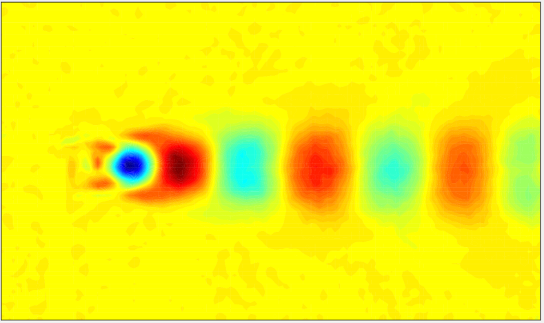
(c) Mode 1, $f_{1}=0.90$ Hz

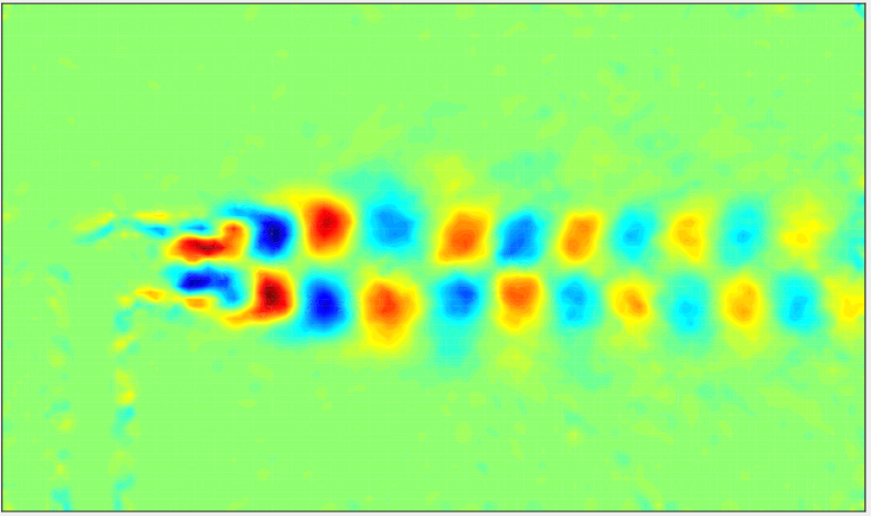
(d) Mode 2, $f_{2}=1.77$ Hz

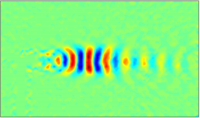
(e) Mode 3, $f_{3}=2.69$ Hz

Figure 6: (a)-(b), Continuous-time DMD eigenvalues (circles) colored by (a) the accuracy criterion $\alpha$ and (b) mode amplitude $\beta$. Mode amplitudes are normalized by the maximum amplitude. Dominant frequencies (blue cross sign $\times$) are shown for comparison. The first 11 eigenvalues that have small $\alpha$ and large $\beta$ are shown (red plus sign $+$). (c)-(e) Three dominant DMD modes (only show real part) picked out by accuracy criterion and mode amplitude.

In this example, we use the experimental particle image velocimetry (PIV) data for flow past a circular cylinder at a Reynolds number of 413. The PIV velocity data was sampled at frequency of 20 Hz with a resolution of $135\times 80$ pixels. See [25] for more details about this experiment. This dataset has been used in other studies [14, 28] for testing various proposed DMD algorithms. We will use vorticity data for DMD, which can be computed from velocity data by finite difference methods. The state dimension is $n=135\times 80=10800$, and the number of snapshots in training data is taken to be $m=1000$. We use an additional $m_{\text{test}}=1000$ snapshot pairs as testing data.

When we apply DMD to sequential data that has time step $\triangle t$, the continuous-time DMD eigenvalues $\lambda_{\text{DMD}}$ are related to the discrete-time DMD eigenvalues $\mu_{\text{DMD}}$ by

$$\mu_{\text{DMD}}=e^{\lambda_{\text{DMD}}\triangle t}.$$ (5.1)

The discrete-time DMD eigenvalues are computed with DMD and converted to continuous-time DMD eigenvalues by equation (5.1), and in this example the time spacing is $\triangle t=(1/20)s$. The DMD frequency $f_{\text{DMD}}$ is related to the continuous-time DMD eigenvalues $\lambda_{\text{DMD}}$ by

$$f_{\text{DMD}}=\frac{\text{Im}(\lambda_{\text{DMD}})}{2\pi},$$ (5.2)

where $\text{Im}(\lambda_{\text{DMD}})$ is the imaginary part of $\lambda_{\text{DMD}}$.

We first apply the standard DMD method described in section 2.1. We use a truncation level $r=100$, which corresponds to preserving $78.16\%$ of the total energy of the snapshots. The continuous-time DMD eigenvalues are shown shaded by the corresponding accuracy criterion values $\alpha$ in Figure 6(a), and time-averaged mode amplitudes $\beta$ in Figure 6(b) (defined as in [16]).

Inspecting Figure 6 (a), we observe that eigenvalues near the imaginary axis are more accurate, and this observation is consistent with physical intuition: this flow exhibits a von Kármán vortex street, whose dominant dynamics evolve on a limit cycle. For this experiment, the wake shedding frequency is $f_{\text{wake}}=0.889$ Hz [25], In previous work [25], the physically relevant dominant frequencies are reported as $f_{0}=0$ Hz, $f_{1}=0.89$ Hz, $f_{2}=1.77$ Hz, $f_{3}=2.73$ Hz. The DMD mode associated with $\lambda_{0}$ is the mean of the flow, and $\lambda_{1},\ \lambda_{2}$ and $\lambda_{3}$ are the first, second, and third harmonic of the fundamental wake frequency $\lambda_{\text{wake}}$. These four frequencies represent the dominant dynamics in this flow. This observation indicates that the proposed accuracy criterion can be used to identify physically relevant DMD modes/eigenvalues, and distinguish relevant modes from irrelevant ones. By comparing Figure 6(a) and (b), we verify that the accuracy criterion indicates the same dominant frequencies as the mode amplitude. The DMD modes that have higher accuracy as indicated by the accuracy criterion are shown in Figure 6(c)-(e). We verify that they look similar to those identified in previous work [25].

KDMD

(a) KDMD, accuracy criterion

(b) KDMD, mode amplitude

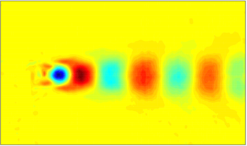
(c) Mode 1, $f_{1}=0.90$ Hz

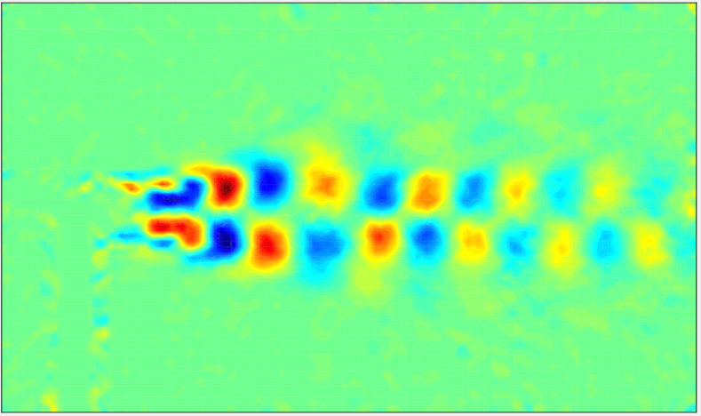
(d) Mode 2, $f_{2}=1.79$ Hz

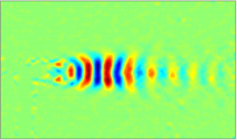
(e) Mode 3, $f_{3}=2.69$ Hz

Figure 7: (a)–(b), Continuous-time KDMD eigenvalues (circles) colored by (a) the accuracy criterion $\alpha$ and (b) mode amplitude $\beta$. Mode amplitudes are normalized by the maximum amplitude. Dominant frequencies (blue cross sign $\times$) are shown for comparison. The first 11 eigenvalues that have small $\alpha$ and large $\beta$ are shown (red plus sign $+$). (c)–(e) Three dominant DMD modes (real part) picked out by accuracy criterion and mode amplitude.

Next, we investigate the performance of KDMD on this dataset. Figure 7 shows results for a polynomial kernel of degree $d=5$, again using a truncation level of $r=100$. The DMD eigenvalues are shown in Figure 7(a)–(b), colored by both accuracy criterion and mode amplitude. The relevant DMD modes picked out by accuracy criterion and mode amplitude are shown in Figure 7(c)–(e). We verify that accuracy criterion is able to isolate dominant modes when using KDMD.

5.2 Canonical separated flow

In this example, we use PIV data from a canonical flow separation experiment sketched in Figure 8. Separation is induced on the surface of a flat plate by a suction/blowing boundary condition imposed on the wall of the wind tunnel, near the trailing edge of the plate. The free-stream velocity is $U_{\infty}=3.9\,\text{m/s}$, the chord length is $c=402$ mm, the span is $s=305$ mm, and the height is $h=0.095c$. The Reynolds number based on chord length is $Re_{c}=10^{5}$, small enough that the boundary layer is likely laminar upstream of the separation point. The average separation bubble length is $L_{\text{sep}}=0.2c$. More information regarding the separation system and the flat plate model can be found in [6].

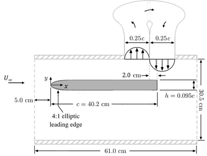
(a) Experiment setup

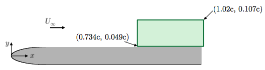
(b) The PIV measurement region

Figure 8: Sketch of the canonical separated flow experiment setup (adapted from [10]) and the PIV measurement region.

PIV velocity data is sampled at $f_{s}=1600$ Hz, with a resolution of $319\times 62$ pixels. The PIV vorticity dataset for the separated flow studied here consists of $m=3000$ snapshot pairs (the training data), with a state dimension $n=319\times 62=19778$. We also take another $m_{\text{test}}=3000$ snapshot pairs as testing data.

(a) TDMD, accuracy criterion

(b) TDMD, mode amplitude

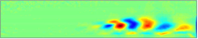
(c) TDMD mode, $f=106$ Hz

Figure 9: TDMD frequency ($f_{\text{TDMD}}$) and corresponding mode error/amplitude. Mode amplitudes are normalized by the maximum mode amplitude. The truncation level is $r=25$. The shear layer frequency $f_{\text{SL}}=106$ Hz is denoted with a red square, and corresponds to the most accurate (smallest $\alpha$) and largest amplitude (largest $\beta$) mode.

This particular experimental dataset has been used and studied in previous work [12], in which the shear layer frequency was found to be $f_{\text{SL}}=106$ Hz. The shear layer frequency is a periodic roll-up of the shear layer due to the Kelvin-Helmholtz instability. The shear layer frequency $f_{\text{SL}}$ can be identified by applying total-least-squares DMD (TDMD), a variant of DMD which makes use of total-least-square regression to improve the accuracy of DMD for noisy data [5, 13]. As in [12], we use a truncation level of $r=25$, which corresponds to preserving $74\%$ of the energy of the data. In this example the time spacing is $\triangle t=1/f_{s}=(1/1600)s$.

For comparison, we also compute the time-averaged mode amplitude $\beta$, as in the example in section 5.1 (e.g., Figure 6(b)). The DMD frequencies are plotted against their accuracy criterion values and mode amplitudes in Figure 9 (a)–(b). It is observed that $f_{\text{SL}}=106$ Hz is accurately identified by TDMD. In addition, it stands out by having a small mode error. The DMD mode associated with shear layer frequency is plotted in Figure 9(c), and it agrees with the mode identified in previous work [12].

KDMD

(a) KDMD, accuracy criterion

(b) KDMD, mode amplitude

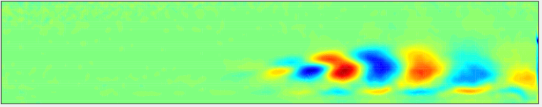
(c) KDMD mode, $f=105$ Hz

Figure 10: KDMD frequency ($f_{\text{KDMD}}$) and corresponding mode error/amplitude. The truncation level is $r=25$. The shear layer frequency $f_{\text{SL}}=106$ Hz is denoted with a red square.

We apply KDMD to this dataset, using polynomial kernels of degree $d=5$, again with a truncation level of $r=25$. Eigenvalue frequencies, and corresponding accuracy criterion values and mode amplitudes are plotted in Figure 10(a)–(b). We observe that the shear layer frequency has small error and large mode amplitude, and once again verify that the DMD mode associated with shear layer frequency (Figure 10(c)) agrees closely with that found in previous work [12].

6 Conclusion and outlook

Exploiting the connection between DMD and the Koopman operator, we have presented an accuracy criterion to evaluate the quality (accuracy) of Koopman eigenpairs approximated with DMD variants. The criterion does not assume access to the analytical Koopman spectral decomposition, which is generally unknown in practice. Furthermore, the proposed accuracy criterion naturally applies to other variants of DMD, because it is based on the general notion of Koopman eigenfunctions. The proposed accuracy criterion is validated with an synthetic system where the analytical Koopman eigenpairs are known. Using this the accuracy criterion, we present a study of the performance of various kernels, and assess their sensitivity to noisy data. In our examples, the polynomial kernel (with finite-dimensional observables) performs well both in the sense of accuracy and robustness to noise. Exponential, Gaussian, and Laplacian kernel are able to span an infinite-dimensional function space, but the tradeoff is that they are significantly more sensitive to noise in the dataset. We demonstrate that the accuracy criterion can assist in identifying accurate and physically relevant DMD modes/eigenvalues from noisy experimental data. The accuracy criterion is conceptually simple and easy to use. As a data-driven algorithm, depending on the nature of the problem, sometimes DMD produces relevant results, and sometimes outputs numerical artifacts. For reduced order modeling based on DMD/Koopman modes, it is hence important to assess the quality of DMD results.

Note that our proposed accuracy criterion requires that some portion of data snapshots be kept out of the DMD analysis for purposes of assessing mode accuracy. However, it would be possible to incorporate this additional data into the DMD analysis after the DMD modes and eigenvalues of interest have been identified.

The demand for accurate reduced order models (ROM) has increased rapidly in recent years, but it is still unclear how to select a subset of Koopman eigenpairs such that the original (nonlinear) system is accurately approximated. In order to build any meaningful ROM we need to at least assess the accuracy and importance of DMD-approximated Koopman eigenpairs. The present work has shed some light on the accuracy side. However, how to select the most dynamically important Koopman eigenpairs remains an open question. Unlike techniques such as Proper Orthogonal Decomposition, in which the modes are orthogonal by construction, Koopman eigenfunctions are in general not orthogonal (though orthogonal DMD-like modes may be obtained [19]). Mode amplitudes obtained by a projection of data onto DMD modes are not necessarily always a meaningful criterion for evaluating importance, as demonstrated in the example in section 3. It would be desirable to develop an importance criterion that can guide the selection of modes for the purpose of representing the dynamics accurately.

References

- [1] S. Bagheri. Effects of weak noise on oscillating flows: Linking quality factor, Floquet modes, and Koopman spectrum. Physics of Fluids, 26:094104, 2014.
- [2] C. M. Bishop. Pattern Recognition and Machine Learning. Springer, 2007.
- [3] K. K. Chen, J. H. Tu, and C. W. Rowley. Variants of dynamic mode decomposition: boundary condition, Koopman, and Fourier analyses. Journal of Nonlinear Science, 22(6):887–915, 2012.
- [4] A. Cotter, J. Keshet, and N. Srebro. Explicit approximations of the Gaussian kernel. arXiv:1109.4603, 2011.
- [5] S. T. M. Dawson, M. S. Hemati, M. O. Williams, and C. W. Rowley. Characterizing and correcting for the effect of sensor noise in the dynamic mode decomposition. Experiments in Fluids, 3(57):1–19, 2016.
- [6] E. Deem, L. Cattafesta, H. Zhang, C. Rowley, M. Hemati, F. Cadieux, and R. Mittal. Identifying dynamic modes of separated flow subject to ZNMF-based control from surface pressure measurements. AIAA Paper 2017-3309, 47th AIAA Fluid Dynamics Conference, 2017.
- [7] D. Duke, J. Soria, and D. Honnery. An error analysis of the dynamic mode decomposition. Experiments in Fluids, 52(2):529–542, 2012.
- [8] G. E. Fasshauer. Positive definite kernels: past, present and future. Dolomite Research Notes on Approximation, 4:21–63, 2011.
- [9] A. Gretton. Introduction to RKHS, and some simple kernel algorithms. Advanced Topics in Machine Learning. Lecture conducted from University College London, 2013.
- [10] J. Griffin, M. Oyarzun, L. N. Cattafesta, J. H. Tu, C. W. Rowley, and R. Mittal. Control of a canonical separated flow. AIAA Paper 2013-2968, 43rd AIAA Fluid Dynamics Conference, 2013.
- [11] D. M. Hawkins. The problem of overfitting. Journal of Chemical Information and Computer Sciences, 44(1):1–12, 2004.
- [12] M. S. Hemati, E. A. Deem, M. O. Williams, C. W. Rowley, and L. N. Cattafesta. Improving separation control with noise-robust variants of dynamic mode decomposition. AIAA Paper 2016-1103, 54th AIAA Aerospace Sciences Meeting, Jan. 2016.
- [13] M. S. Hemati, C. W. Rowley, E. A. Deem, and L. N. Cattafesta. De-biasing the dynamic mode decomposition for applied koopman spectral analysis of noisy datasets. Theoretical and Computational Fluid Dynamics, pages 1–20, 2017.
- [14] M. S. Hemati, M. O. Williams, and C. W. Rowley. Dynamic mode decomposition for large and streaming datasets. Physics of Fluids, 26(11):111701, 2014.
- [15] M. R. Jovanović, P. J. Schmid, and J. W. Nichols. Sparsity-promoting dynamic mode decomposition. Physics of Fluids, 26(2):024103, 2014.
- [16] J. Kou and W. Zhang. An improved criterion to select dominant modes from dynamic mode decomposition. European Journal of Mechanics-B/Fluids, 62:109–129, 2017.
- [17] J. N. Kutz, S. L. Brunton, B. W. Brunton, and J. L. Proctor. Dynamic Mode Decomposition: Data-Driven Modeling of Complex Systems, volume 149. SIAM, 2016.
- [18] J. Mercer. Functions of positive and negative type, and their connection with the theory of integral equations. Philosophical Transactions of the Royal Society of London, Series A, 209:415–446, 1909.
- [19] B. R. Noack, W. Stankiewicz, M. Morzyński, and P. J. Schmid. Recursive dynamic mode decomposition of transient and post-transient wake flows. Journal of Fluid Mechanics, 809:843–872, 2016.
- [20] C. W. Rowley and S. T. Dawson. Model reduction for flow analysis and control. Annual Review of Fluid Mechanics, 49(1), 2017.
- [21] C. W. Rowley, I. Mezić, S. Bagheri, P. Schlatter, and D. S. Henningson. Spectral analysis of nonlinear flows. Journal of Fluid Mechanics, 641:115–127, 2009.
- [22] P. J. Schmid. Dynamic mode decomposition of numerical and experimental data. Journal of Fluid Mechanics, 656:5–28, 2010.
- [23] C. Scovel, D. Hush, I. Steinwart, and J. Theiler. Radial kernels and their reproducing kernel Hilbert spaces. Journal of Complexity, 26(6):641–660, 2010.
- [24] C. R. Souza. Kernel functions for machine learning applications. Creative Commons Attribution-Noncommercial-Share Alike, 3, 2010.
- [25] J. H. Tu, C. W. Rowley, J. N. Kutz, and J. K. Shang. Spectral analysis of fluid flows using sub-Nyquist-rate PIV data. Experiments in Fluids, 55(9):1–13, 2014.
- [26] J. H. Tu, C. W. Rowley, D. M. Luchtenburg, S. L. Brunton, and J. N. Kutz. On dynamic mode decomposition: Theory and applications. Journal of Computational Dynamics, 1(2):391–421, 2014.
- [27] M. O. Williams, I. G. Kevrekidis, and C. W. Rowley. A data–driven approximation of the Koopman operator: Extending dynamic mode decomposition. Journal of Nonlinear Science, 25(6):1307–1346, 2015.
- [28] M. O. Williams, C. W. Rowley, and I. G. Kevrekidis. A kernel-based method for data-driven Koopman spectral analysis. Journal of Computational Dynamics, 2(2):247–265, 2015.
- [29] A. Wynn, D. Pearson, B. Ganapathisubramani, and P. Goulart. Optimal mode decomposition for unsteady flows. Journal of Fluid Mechanics, 733:473, 2013.
- [30] H. Zhang, C. W. Rowley, E. A. Deem, and L. N. Cattafesta. Online dynamic mode decomposition for time-varying systems. arXiv:1707.02876, 2017.