Small scale exact coherent structures at large Reynolds numbers in plane Couette flow

Abstract

The transition to turbulence in plane Couette flow and several other shear flows is connected with saddle node bifurcations in which fully 3-d, nonlinear solutions, so-called exact coherent states (ECS), to the Navier-Stokes equation appear. As the Reynolds number increases, the states undergo secondary bifurcations and their time-evolution becomes increasingly more complex. Their spatial complexity, in contrast, remains limited so that these states cannot contribute to the spatial complexity and cascade to smaller scales expected for higher Reynolds numbers. We here present families of scaling ECS that exist on ever smaller scales as the Reynolds number is increased. We focus in particular on two such families for plane Couette flow, one centered near the midplane and the other close to a wall. We discuss their scaling and localization properties and the bifurcation diagrams. All solutions are localized in the wall-normal direction. In the spanwise and downstream direction, they are either periodic or localized as well. The family of scaling ECS localized near a wall is reminiscent of attached eddies, and indicates how self-similar ECS can contribute to the formation of boundary layer profiles.

1 Introduction

Pipe flow and various other parallel and non-parallel shear flows show a transition to turbulence that is not connected to a linear instability of the laminar profile [Grossmann:2000]. The transition can be triggered by finite amplitude bifurcations and the new states that emerge are spatially and temporally fluctuating. The origin of the transition and the subsequent dynamics cannot be understood within linear approximations but require that the nonlinearity of the Navier-Stokes equation is taken into account. Underlying the complex spatio-temporal patterns are exact coherent states (ECS) [Waleffe:1998wk, Waleffe:2001wu], i.e. velocity fields that are solutions to the Navier-Stokes equation with a relatively simple temporal dynamics: they can be fixed points of the equations of motion, travelling waves or more complex relative periodic orbits [Eckhardt:2007ix, Kerswell:2005ir, Eckhardt:2007ka]. ECS provide nuclei for the formation of turbulence. They typically appear in saddle-node bifurcations [Mellibovsky:2011gq] and then undergo sequences of secondary bifurcations that give temporally complex dynamics [Kreilos:2012bd, Avila:2013jq, Zammert:2015jg]. Crisis bifurcations can change the dynamics from persistent to transient, and collisions between different coherent structures can set up a network that sustains long-lived turbulent dynamics [Hof:2006ab, Hof:2008cb, Avila:2010ep, Schneider:2010gv, Kreilos:2014ew].

The bifurcations just described follow the patterns familiar from the various routes to chaos and can explain the temporally complex dynamics [Eckmann:1981kw, Ott:2002wz]. In order to realize the distribution of energy to ever smaller scales that are the hallmark of fully developed turbulence [Frisch:1995wl] mechanisms that create structures on smaller scales are required. Steps towards developed turbulence are described in the studies of [Kawahara:2001ft] where it is shown that ECS can capture some of the turbulent dynamics, and [vanVeen:2009fm], where coherent structures for models of homogeneous turbulence are described. In all cases the Reynolds numbers are moderate and the structures remain large-scale in the sense that they extend all the way across the available volume. The examples presented below belong to families of states that can be scaled to ever finer spatial scales as the Reynolds number increases.

All ECS are fully three-dimensional: all velocity components are active and they vary in all three directions. Simpler structures, e.g. with translational invariance in the downstream direction, decay [Moffatt:1990fb]. Many of them share relatively stable relations between their height, width, and downstream periodicity: if $H$ denotes the height, then the width of the structures is about $\pi H$ and the downstream wavelength is about $2\pi H$. For plane Couette flow, the exact optimal relations are documented in [Clever:1997tq, Waleffe:2003hh], and the estimates for pipe flow are given in [Faisst:2003hd, Eckhardt:2008jv, Pringle:2009fe]. Similar results are available for plane Poiseuille flow, though the optimal wavelength described in [Zammert:2016fk] shows that there is some variability in the optimal ratios. All ECS just described span across the entire height of the shear flow.

An approach to finding smaller structures is suggested by the behaviour of states in pipe flow [Faisst:2003hd, Eckhardt:2008jv, Pringle:2009fe]: as number of vortices along the circumference increases, they move closer to the walls and also their downstream wavelength decreases. Apparently, the vortices try to maintain the geometric relations as they become narrower. This observation suggests that smaller structures can be obtained by scaling structures in all three directions, and specifically by prescribing the spanwise wavelength, so that the extension of the states in the normal and downstream direction has to adjust to the prescribed widths. [Hall:2010cn] noted such a scaling for states in their asymptotic expansion for high Reynolds numbers and [Deguchi:2015gu] showed that this is one of the scalings inherent in this expansion. Here, we employ this scaling to find approximate rescaled states that are then refined using a Newton step to arrive at a state that is an ECS of the full Navier-Stokes equation at a prescribed Reynolds number. We apply this to several states from plane Couette flow, trace them to high Reynolds numbers, and show their bifurcation and scaling properties. Of particular interest are a set of structures that are localized near the walls and which can be viewed as ECS that may support the popular image of boundary layers being carried by a hierarchy of eddies attached to the walls [Townsend:1980uj, Perry:1991ab, Perry:1994ab].

In the next section, we present the scaling ansatz for plane Couette flow. In section 3, we discuss the properties of states. We first focus on states that are periodic in the spanwise and downstream direction, and that are localized in the center (section 3.1) and near a wall (section 3.2). We then describe their bifurcation and scaling structure (section 3.3), their localization in the normal direction (section 3.4) and their stability properties (section 3.5). States that are also localized in the downstream or spanwise direction are described in section 4. Conclusions are given in section 5.

2 Scaling in plane Couette flow

The flow we consider here is plane Couette flow, the flow between two parallel plates moving relative to each other. With $x$ the downstream direction, $y$ the normal direction, and $z$ the spanwise direction, the laminar profile is $\mathbf{u}_{0}(x,y,z)=Sy$ with the shear $S=U_{0}/d$ for plates at $y=\pm d$ that move with velocity $\pm U_{0}$. Deviations $\mathbf{u}$ from the laminar profile then satisfy the equation

$$\partial_{t}\mathbf{u}+(Sy\mathbf{e}_{x}\cdot\nabla)\mathbf{u}+(\mathbf{u}\cdot\nabla)Sy\mathbf{e}_{x}+(\mathbf{u}\cdot\nabla)\mathbf{u}+\nabla p=\nu\Delta\mathbf{u}\,.$$ (1)

with $\nu$ the kinematic viscosity. For stationary states, $\partial_{t}\mathbf{u}=0$ and only the spatial degrees of freedom remain. For states moving with a constant phase velocity $c$ in the downstream direction, transition to a comoving frame $\tilde{x}=x-ct$ gives $\partial_{t}\mathbf{u}=-c\partial_{x}\mathbf{u}$ and a time-independent equation in $\tilde{x}$.

Let $\mathbf{u}_{0}(\mathbf{x})$ be a solution to the stationary equation for a viscosity $\nu_{0}$. Then the scaled velocity field

$$\mathbf{u}_{\lambda}(\mathbf{x})=\mathbf{u}_{0}(\lambda\mathbf{x})/\lambda$$ (2)

satisfies

$$-c^{*}\partial_{x}\mathbf{u}_{0}+(Sy^{*}\mathbf{e}_{x}\cdot\nabla)\mathbf{u}_{0}+(\mathbf{u}_{0}\cdot\mathbf{e}_{y})S\mathbf{e}_{x}+(\mathbf{u}_{0}\cdot\nabla)\mathbf{u}_{0}+\nabla p^{*}=\nu^{*}\Delta\mathbf{u}_{0}$$ (3)

in the scaled coordinates $\mathbf{x}^{*}=\lambda\mathbf{x}$ with $c^{*}=c\lambda$ and $\nu^{*}=\nu/\lambda^{2}$. That is to say, $\mathbf{u}_{\lambda}$ is a solution at the modified viscosity $\nu^{*}$. With this transformation, we also have to adjust the walls, and they move outwards at the same rate, $d^{*}=d\lambda$. However, if the state is localized in the normal direction, the velocity fields will decay towards the walls and the specific location of the walls will only have a small influence on the state. By the above heuristics, the state will be localized in the normal direction if the spanwise and/or downstream periodicity are small compared to the initial distance between the walls.

To see the scaling in Reynolds number, we define $\mbox{Re}=(Sd)d/\nu$, so that the rescaled state $\mathbf{u}_{\lambda}$ are equilibrium states for

$$\mbox{Re}^{*}=\lambda^{2}\mbox{Re}_{0}.$$ (4)

or, alternatively, that a solution at Reynolds number $\mbox{Re}^{*}$ can be obtained with the rescaling

$$\lambda=\sqrt{\frac{\mbox{Re}^{*}}{\mbox{Re}_{0}}}.$$ (5)

from a solution at Reynolds number Re. The scaling would be exact if the walls were infinitely far away. In the presence of the walls, the scaled states can be taken as initial conditions in a Newton refinement and ECS on the new scales can be obtained.

For the numerical simulations we use Gibson’s Channelflow-code [Gibson2009b] and the optimized Newton methods for the determination of ECS. As a starting point, we use two equilibrium solution that are similar to Eq1 and Eq7 of [Gibson:2009kp], which differ in their vortical content. They will collectively be referred to as EQ when they are turned into equilibrium solutions in the center and as TW when they are scaled as travelling waves near walls.

3 Families of scaling solutions in plane Couette flow

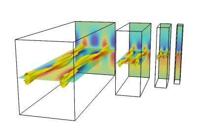
Figure 1: Visualization of the exact solutions localized in the center of the channel for Reynolds number $100,000$. The four solutions are scaled in width and length by factors of $2$, $4$, and $8$. The yellow surfaces show iso-contours of the Q-vortex criterion. The streamwise velocity component is color coded from low values (blue) to high values (red) in the mid plane cutting through the structure and in the plane at the back of the domain.

3.1 Stationary states in the center

We begin with solutions that are localized in the center of the domain and stationary so that $c=0$. The initial computational domain has spanwise and streamwise periodicity of $0.5\pi$ and $1.5\pi$, respectively, and a height of $2$. Consistent with previous analysis, we can determine the state accurately with a resolution $N_{x}\times N_{y}\times N_{z}=32\times 97\times 48$ near $Re^{*}=650$. For higher Reynolds numbers, the resolution has to be increased, e.g. at $Re_{0}=10^{5}$ we use a resolution $N_{x}\times N_{y}\times N_{z}=24\times 185\times 56$. At each Re we carefully checked convergence and that the used resolution is sufficient.

Although the rescaling works for any value of $\lambda$, we will here study powers of two only. Thus, using scaling factors $\lambda$ of $2$, $4$ and $8$, we can identify equilibrium solutions that are reduced in size by factors $2$, $4$, and $8$ in all three directions. The corresponding Reynolds numbers increase by factors of 4, 16, and 64. The stationary state is initially identified at Reynolds number near $3000$, and then scaled up in Reynolds number to higher values up to $192,000$. In order to be able to compare the states at a prescribed Reynolds number, the states are then traced to a Reynolds number $\mbox{Re}=100,000$. Visualizations for the states in the center are shown in Figure 1.

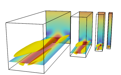
Figure 2: Visualization of the lower branch states of exact solutions near the lower wall, at Reynolds number $\mbox{Re}=100,000$. The representation is the same as in Fig. 1.

3.2 Stationary states near a wall

For the structures localized in the center, the midplane where $c=0$ is a good point of reference, and scaling by $\lambda$ moves the boundary planes further away. For states close to a wall, the point of reference has to be the wall. Eventually, the state will move closer to the wall and the phase speed will approach $\pm U_{0}$, the speed of the wall. Accordingly, we shift the domain upwards by $d$ and change to a co-moving frame of reference where $U(y=0)=0$ and $U(y=2d)=2U_{0}$. The equation for the stationary state remains similar to (3).

The spanwise and streamwise wavelengths of the initial domain are $0.4\pi$ and $0.877\pi$, respectively. The scaled states are shown in Figure 2. This family of ECS is reminiscent of the structures used in attached eddy models for the logarithmic layer in wall turbulence, where the flow field is modeled by a hierarchy of eddies which are attached to the wall and whose dimensions increase with the distance to the wall [Woodcock:2015ut].

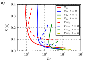
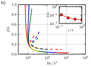
Figure 3: Bifurcation diagrams for the scaled ECS in the center (derived from $EQ$, full lines) and near the wall (derived from $TW$, dashed lines). (a) shows the unscaled bifurcation diagrams and (b) the rescaled ones where a collapse of the data is observed. The inset in (b) shows the rescaled dissipation of the wall states at $Re=10^{5}$ versus the scaling parameter $\lambda$.

3.3 Bifurcation diagrams

A bifurcation diagram using the volume averaged dissipation,

$$D(\mathbf{u})=\frac{1}{2L_{x}L_{z}}\int_{0}^{L_{z}}\int_{-1}^{1}\int_{0}^{L_{x}}\|\nabla\times\mathbf{u}\|^{2}dxdydz,$$ (6)

along the ordinate is given in figure 3a. If one uses the rescaled dissipation on the abscissa and the rescaled Reynolds number $\mbox{Re}^{*}=\lambda^{2}Re_{0}$ on the ordinate the bifurcation curves should collapse. Indeed, in the rescaled bifurcation diagram shown in figure 3b) the collapse of the bifurcation curves for different $\lambda$ is very good.

At a fixed Reynolds number the volume averaged dissipation (eqn. 6) decreases with $\lambda$. But the states also become smaller with increasing $\lambda$, filling only a fraction $1/\lambda$ of the domain in the wall-normal direction, so that the rescaled dissipation $\lambda D$ is a better measure for the dissipation and its scaling. At fixed value of Re the rescaled dissipation increases with $\lambda$, as shown for $TW$ and $Re=10^{5}$ and $1.2\cdot 10^{5}$ in the inset in Figure 3b).

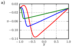
Figure 4: Profiles for $TW_{w}$ in the original coordinates (left column) and in wall units (right column). The linear laminar profile has been subtracted. (a) Profile of the streamwise velocity. (b) Rescaled velocity profile. c) Profiles in the cross flow energy density $e_{CF}$ as measure for the location of vortices. d) Rescaled profile of $e_{CF}$ in wall units.

3.4 Localization properties in the normal direction

Scaling of the solutions requires that in the normal direction they are not or only weakly influenced by the walls. In wall bounded flows, distances and velocities are usually measured in wall units, based on the viscosity and the friction velocity $u_{\tau}$. The wall friction is given by

$$\tau=\nu\left\langle\frac{\partial u_{x}}{\partial_{y}}\right\rangle_{w}$$ (7)

where the index $w$ indicates an average at the wall. Then the units for velocity are $u_{\tau}=\sqrt{\tau}$ and $\ell_{\tau}=\nu/u_{\tau}$. With the scaling of the ECS given by (2) and the scaling of the viscosity, one finds that the scales at two Reynolds numbers $\mbox{Re}^{*}$ and $\mbox{Re}_{0}$ (as in (5)) are related by

$$\tau^{*}=\frac{1}{\lambda^{2}}\tau_{0}\qquad u_{\tau}^{*}=\frac{1}{\lambda}u_{\tau}^{(0)}\qquad\ell_{\tau}^{*}=\frac{1}{\lambda}\ell_{\tau}^{(0)}$$ (8)

Therefore, the rescaling of velocities and lengths by $\lambda$ is equivalent to a rescaling to wall units if the solutions scale exactly. Since we have to adjust the solutions a little bit in order to obtained converged states at the respective Reynolds numbers, there are small deviations in the friction factors, and hence in the wall units. Specifically, for the cases shown here, $l_{\tau}$ varies between $3.02\cdot 10^{-3}$ for the largest state with $\lambda=1$ and $3.13\cdot 10^{-3}$ for the smallest state with $\lambda=8$, all evaluated at Reynolds number $\mbox{Re}=100,000$.

The mean downstream velocity the profiles for the wall states are shown in the top row of Figure 4. With increasing $\lambda$ the states become ever more localized near the wall and the maximal amplitude becomes smaller. However, from the maximum to the upper wall, the decay is very slow and essentially linear, as shown in the rescaled solution in the right column.

Other measures provide a much clearer signal for the localization. For instance, the cross flow energy density,

$$e_{CF}(y)=\frac{1}{L_{x}L_{z}}\int_{0}^{L_{x}}\int_{0}^{L_{x}}\left(v^{2}+w^{2}\right)dxdz,$$ (9)

which is shown in Figure 4c, decays much faster outside the region where the vortices are located. The rescaled curves for the cross flow energy density (Figure 4d) collapse perfectly and reveal the similarity of the solutions. In the normal direction, the ECS modify the mean velocity within the structure, but do not provide any forces further away. In the absence of forces, the laminar shear profile is linear, which shows that the linear profile in the outer region is a consequence of the viscous mediation between the downstream velocity at the outer edge of the ECS and the velocity at the upper wall.

In the other directions, one can adapt the model for streamwise localization in plane Couette flow [Brand:2014he, Barnett:2016ty] to show that ECS are exponentially localized in the streamwise direction. In the spanwise direction, the decay seems to be somewhat stronger, as also noticed for large scale ECS [Schneider:2010id].

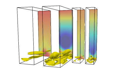
Figure 5: Comparison of the lower (a,c) and upper (b,d) branch states for the solutions localized near the lower wall. For the left pair of figures (a,b) the Reynolds number is $18,200$ and for the right pair (c,d) it is $52,000$. The yellow surfaces are iso-contours of the Q-vortex criterion. The used value of Q is $0.002$ for (a,b) and $Q=0.005$ for (c,d). In the back-plane the streamwise velocity component is color-coded. The minimal (blue) and maximal (red) values of $u$ are $-0.3$ and $0.05$ in (a,b) and $-0.16$ and $0.05$ in (c,d), respectively.

The upper branch states for both solutions have a much larger wall-normal extension than the lower branches states (see Figure 5). Thus, they are more strongly influenced by the wall which causes an imperfect scaling, especially for low values of $\lambda$. For larger $\lambda$ the range of the upper branch states in the wall normal direction decreases, resulting in better scaling.

For both the states in the center and near the wall, the lower branch shows less variation in streamwise direction with increasing distance to the bifurcation point, which is a common feature of lower branch states [Wang2007, Gibson2014].

3.5 Stability properties

In order to analyze the stability properties of the scales states the eigenvalues of the ECS are calculated in computational domains with spatial periodicities equal to those of the states. The leading eigenvalues are shown in Figure 6. All states are unstable, but the number of unstable eigenvalues is rather low. The result show that the leading eigenvalues of states whose Reynolds numbers differ by the scaling factor $\lambda$, the leading eigenvalues are almost identical. This is a consequence of the scaling in (3), which leave the time-dependence invariant. Thus, the dynamics close to the ECS is similar in the adjusted domains.

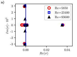
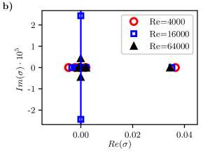
Figure 6: Stability properties of the rescaled ECS. (a) Real and imaginary parts of the leading eigenvalues for $EQ$ at $Re=5850$ and the scaled solutions for $\lambda=2$ and $4$ at $Re=23400$ and $Re=93600$. b) Leading eigenvalues for $TW$ at $Re=4000$ and the scaled solutions for $\lambda=2$ and $4$ at $Re=16,000$ and $Re=64,000$.

4 Spanwise and streamwise localization

In addition to the ECS in domains that are periodic in the downstream and spanwise direction, we also tracked states that are localized in these directions [Schneider:2010id, Schneider:2010jz]. As in other cases, good initial guesses can be be obtained by applying suitable window functions to extract nuclei for localized states from spatially extended states [Gibson2014]. We demonstrate this for one streamwise and two spanwise localized equilibrium solutions which are related to $EQ$ and $TW$.

Figure 7 shows visualizations of a streamwise localized equilibrium state related to $EQ$, and of the corresponding scaled solutions. As for the streamwise extended solutions, the visualizations for the different values of $\lambda$ look very similar because the scaling works quite well. The bifurcation diagram of the streamwise localized states is more complicated than for the spatially extended states. In particular, it has not been possible to trace the family of scaled states to a common fixed value of Re. They are therefore visualized at different Reynolds numbers that differ approximately by a factor $\lambda^{2}=4$.

The figure shows that the vortex tubes are oriented in a V-shape which is also a feature of the recently identified doubly localized equilibrium states of PCF [Brand2014]. The states show an exponential decay of the velocity components in their tails. Models for the streamwise decay length $\ell$ in an exponential representation $u\propto\exp(-|x|/\ell)$ of the downstream variation show that $\ell$ increases with Reynolds number but decreases with spanwise wavelength [Brand2014, Zammert2016c]. For the rescaled ECS studied here this means that the stretching of $\ell$ due to the increase in Reynolds number is compensated by the reduction of the lateral scales so that the overall all directions can be rescaled by $\lambda$.

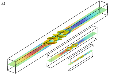
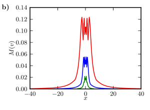
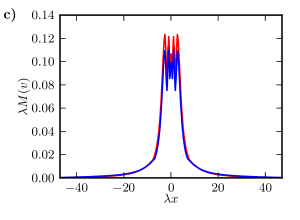
Figure 7: Streamwise localized equilibrium solutions. (a) Visualizations of the flow fields at Reynolds numbers $900$, $3750$, and $15600$. The streamwise and spanwise lenghts of the largest domain are $7.5\pi$ and $0.5\pi$, respectively. (b) Maximum of the wall-normal velocity component $M(v)$ versus the streamwise position $x$ for the three localized equilibrium solutions. (c) $M(v)$ rescaled by $\lambda$. Note that the green line is covered by the blue one, showing the almost perfect scaling for high Reynolds number.

5 Conclusions

The tracking of ECS from large scales to ever smaller scales at increasing Reynolds numbers show that a multitude of small-scale ECS populate the state space of flows at high Reynolds numbers. Their localization in the wall-normal direction show that similar states can also appear in shear flows with curvature in the mean profile, such as Poiseuille flow, since eventually the states will only probe the local shear gradient [Deguchi:2015gu].

The two cases studied here are located at the midplane of the domain, where the mean velocity is $0$, and near the walls, where the mean advection speed approaches the speed of the wall. For states at some distance to the wall, one can keep that distance fixed and scale the states so that they become localized at that height. Initially, for low Reynolds numbers, there will be some influence of the walls, but then for higher Reynolds numbers and more localized states, the influence from the walls will become smaller, and one can anticipate that the states become similar to the ones in the center.

The localization in the normal direction, and also in the other directions, implies that sets of states can be combined to form ECS of more complex spatial structures: for superpositions of localized states the nonlinear terms are weak if they are very far apart, and even if the interactions between the two states are stronger, the superposition provides a good starting point for a Newton method. In the few cases where we attempted such superpositions, the Newton method was able to adjust the flow fields so that converged ECS that are have two (or more) centers of localization could be obtained.

For the staggered attached eddies used to represent boundary layers [Perry:1991ab, Perry:1994ab] a simple superposition will not work because the states overlap not only in their fringes but in their core. The interactions will then be more complicated than the simple perturbative adjustment that worked for spatially separated structures, and remains a challenge for computations. Without that interaction, the wall states can be used to form approximate hierarchical superpositions of structures of the type discussed in [Woodcock:2015ut]. Therefore, the wall states described here are a promising starting point for modelling hierarchical structures near walls.

The similarity of the stability properties of the rescaled ECS in the rescaled domain suggests that the frequency with which ECS are visited, which is directly related to their instability, is preserved under scaling. Therefore, the small scale ECS should be visited and be visible in the flows on that scale as frequently as on the large scale. Indeed, DNS simulations in narrow domains [Yang:2017up] show structures that are similar to the ones described here. In an extensive data analysis of homogeneous shear flows, [Dong:2017cd] deduced structures consisting of vortex and streaks which they termed roller states. They are similar to one half of the ECS shown in Figure 1. Two such states can be combined to form a stationary states, which is consistent with the observation that the ECS are stationary states, whereas the roller states of Dong et al are transient. Nevertheless, the similarity between ECS and observations in DNS is encouraging and shows that it is possible to detect ECS not only in low-Re transitional flows [Hof:2004ab, Schneider:2007ib, Kerswell:2007ds] but also in high-Reynolds number situations. It should therefore also be possible to extend the use of ECS for the characterization of transitional flows to fully developed turbulent flows and to provide, for instance, a dynamical basis for the attached eddy hypothesis.

Finally, we note that the structures described here should also be observed in the presence of curved walls: when the Reynolds number increases the curvature becomes small on the scale of the structures and hence negligible. So very close to the wall in pipe flow, or in Görtler flow, similar structures should appear.

References

References

- [1] \harvarditemAvila et al.2013Avila:2013jq Avila M, Mellibovsky F, Roland N \harvardand Hof B 2013 Phys. Rev. Lett. 110(22), 224502.
- [2] \harvarditemAvila et al.2010Avila:2010ep Avila M, Willis A P \harvardand Hof B 2010 J. Fluid Mech. 646, 127.
- [3] \harvarditemBarnett et al.2016Barnett:2016ty Barnett J, Gurevich D R \harvardand Grigoriev R O 2017 Phys. Rev. E 95, 033124.
- [4] \harvarditemBrand \harvardand Gibson2014aBrand:2014he Brand E \harvardand Gibson J F 2014a J. Fluid Mech. 750, R3.
- [5] \harvarditemBrand \harvardand Gibson2014bBrand2014 Brand E \harvardand Gibson J F 2014b J. Fluid Mech. 750, R1.
- [6] \harvarditemClever \harvardand Busse1997Clever:1997tq Clever R M \harvardand Busse F H 1997 J. Fluid Mech. 344, 137–153.
- [7] \harvarditemDeguchi2015Deguchi:2015gu Deguchi K 2015 J. Fluid Mech. 781, R6.
- [8] \harvarditemDong et al.2017Dong:2017cd Dong S, Lozano-Durán A, Sekimoto A \harvardand Jiménez J 2017 J. Fluid Mech. 816, 167–208.
- [9] \harvarditemEckhardt2007Eckhardt:2007ix Eckhardt B 2007 Nonlinearity 21(1), T1–T11.
- [10] \harvarditemEckhardt et al.2008Eckhardt:2008jv Eckhardt B, Faisst H, Schmiegel A \harvardand Schneider T M 2008 Phil. Trans. R. Soc. A 366(1868), 1297–1315.
- [11] \harvarditemEckhardt et al.2007Eckhardt:2007ka Eckhardt B, Schneider T M, Hof B \harvardand Westerweel J 2007 Annu. Rev. Fluid. Mech. 39(1), 447–468.
- [12] \harvarditemEckmann1981Eckmann:1981kw Eckmann J P 1981 Rev. Mod. Phys. 53(4), 643–654.
- [13] \harvarditemFaisst \harvardand Eckhardt2003Faisst:2003hd Faisst H \harvardand Eckhardt B 2003 Phys. Rev. Lett. 91(22), 224502.
- [14] \harvarditemFrisch1995Frisch:1995wl Frisch U 1995 Turbulence The Legacy of A. N. Kolmogorov Cambridge University Press.
-
[15]
\harvarditemGibson2012Gibson2009b
Gibson J F 2012 Channelflow: a spectral Navier-Stokes simulator in C++
Technical report U. New Hampshire.
\harvardurlchannelflow.org - [16] \harvarditemGibson \harvardand Brand2014Gibson2014 Gibson J F \harvardand Brand E 2014 J. Fluid Mech. 745, 25–61.
- [17] \harvarditemGibson et al.2009Gibson:2009kp Gibson J F, Halcrow J \harvardand Cvitanović P 2009 J. Fluid Mech. 638, 243.
- [18] \harvarditemGrossmann2000Grossmann:2000 Grossmann S 2000 Rev. Mod. Phys. 72(2), 603–618.
- [19] \harvarditemHall \harvardand Sherwin2010Hall:2010cn Hall P \harvardand Sherwin S 2010 J. Fluid Mech. 661, 178–205.
- [20] \harvarditemHof et al.2008Hof:2008cb Hof B, de Lozar A, Kuik D \harvardand Westerweel J 2008 Phys. Rev. Lett. 101(21), 214501.
- [21] \harvarditemHof et al.2004Hof:2004ab Hof B, van Doorne C W H, Westerweel J, Nieuwstadt F T M, Faisst H, Eckhardt B, Wedin H, Kerswell R R \harvardand Waleffe F 2004 Science 305(5), 1594–1598.
- [22] \harvarditemHof et al.2006Hof:2006ab Hof B, Westerweel J, Schneider T M \harvardand Eckhardt B 2006 Nature 443(7107), 59–62.
- [23] \harvarditemKawahara \harvardand Kida2001Kawahara:2001ft Kawahara G \harvardand Kida S 2001 J. Fluid Mech. 449, 291.
- [24] \harvarditemKerswell2005Kerswell:2005ir Kerswell R R 2005 Nonlinearity 18(6), R17–R44.
- [25] \harvarditemKerswell \harvardand Tutty2007Kerswell:2007ds Kerswell R R \harvardand Tutty O R 2007 J. Fluid Mech. 584, 69.
- [26] \harvarditemKreilos \harvardand Eckhardt2012Kreilos:2012bd Kreilos T \harvardand Eckhardt B 2012 Chaos 22(4), 047505.
- [27] \harvarditemKreilos et al.2014Kreilos:2014ew Kreilos T, Eckhardt B \harvardand Schneider T M 2014 Phys. Rev. Lett. 112(4), 044503.
- [28] \harvarditemMellibovsky \harvardand Eckhardt2011Mellibovsky:2011gq Mellibovsky F \harvardand Eckhardt B 2011 J. Fluid Mech. 670, 96–129.
- [29] \harvarditemMoffatt1990Moffatt:1990fb Moffatt H K 1990 in ‘Whither Turbulence? Turbulence at the Crossroads: Proceedings of a Workshop Held at Cornell University’ Department of Applied Mathematics and Theoretical Physics pp. 250–257.
- [30] \harvarditemOtt2002Ott:2002wz Ott E 2002 Chaos in Dynamical Systems Cambridge University Press.
- [31] \harvarditemPerry et al.1991Perry:1991ab Perry A E, Li J D \harvardand Marusic I 1991 Philosophical Transactions: Physical Sciences and Engineering 336(1), 67–79.
- [32] \harvarditemPerry et al.1994Perry:1994ab Perry A E, Marusic I \harvardand Li J D 1994 Phys. Fluids A 6(2), 1024–1035.
- [33] \harvarditemPringle et al.2009Pringle:2009fe Pringle C C T, Duguet Y \harvardand Kerswell R R 2009 Phil. Trans. R. Soc. A 367(1888), 457–472.
- [34] \harvarditemSchneider et al.2010Schneider:2010gv Schneider T M, De Lillo F, Buehrle J, Eckhardt B, Dörnemann T, Dörnemann K \harvardand Freisleben B 2010 Phys. Rev. E 81(1), 015301.
- [35] \harvarditemSchneider et al.2007Schneider:2007ib Schneider T M, Eckhardt B \harvardand Vollmer J 2007 Phys. Rev. E 75(6), 066313.
- [36] \harvarditemSchneider, Gibson \harvardand Burke2010Schneider:2010jz Schneider T M, Gibson J F \harvardand Burke J 2010 Phys. Rev. Lett. 104(10), 104501.
- [37] \harvarditemSchneider, Marinc \harvardand Eckhardt2010Schneider:2010id Schneider T M, Marinc D \harvardand Eckhardt B 2010 J. Fluid Mech. 646, 441.
- [38] \harvarditemTownsend1980Townsend:1980uj Townsend A A 1980 The Structure of Turbulent Shear Flow Cambridge University Press.
- [39] \harvarditemvan Veen et al.2009vanVeen:2009fm van Veen L, Kida S \harvardand Kawahara G 2009 Fluid Dyn. Res. 38(1), 19–46.
- [40] \harvarditemWaleffe1998Waleffe:1998wk Waleffe F 1998 Phys. Rev. Lett. 81(19), 4140.
- [41] \harvarditemWaleffe2001Waleffe:2001wu Waleffe F 2001 J. Fluid Mech. 435, 93–102.
- [42] \harvarditemWaleffe2003Waleffe:2003hh Waleffe F 2003 Phys. Fluids A 15(6), 1517.
- [43] \harvarditemWang et al.2007Wang2007 Wang J, Gibson J F \harvardand Waleffe F 2007 Phys. Rev. Lett. 98, 204501.
- [44] \harvarditemWoodcock \harvardand Marusic2015Woodcock:2015ut Woodcock J D \harvardand Marusic I 2015 Phys Fluids A 27, 015104.
- [45] \harvarditemYang et al.2017Yang:2017up Yang Q, Willis A P \harvardand Hwang Y 2017 J. Fluid Mech. pp. 1–24.
- [46] \harvarditemZammert \harvardand Eckhardt2015Zammert:2015jg Zammert S \harvardand Eckhardt B 2015 Phys. Rev. E 91(4), 041003.
- [47] \harvarditemZammert \harvardand Eckhardt2016aZammert:2016fk Zammert S \harvardand Eckhardt B 2016a J. Turbul. 18(2), 103–114.
- [48] \harvarditemZammert \harvardand Eckhardt2016bZammert2016c Zammert S \harvardand Eckhardt B 2016b Phys. Rev. E 94, 041101(R).
- [49]