Excited cosmic strings with superconducting currents

Abstract

We present a detailed analysis of excited cosmic string solutions which possess superconducting currents. These currents can be excited inside the string core, and – if the condensate is large enough – can lead to the excitations of the Higgs field. Next to the case with global unbroken symmetry, we discuss also the effects of the gauging of this symmetry and show that excited condensates persist when coupled to an electromagnetic field. The space-time of such strings is also constructed by solving the Einstein equations numerically and we show how the local scalar curvature is modified by the excitation. We consider the relevance of our results on the cosmic string network evolution as well as observations of primordial gravitational waves and cosmic rays.

I Introduction

Although cosmic strings Nielsen and Olesen (1973); Kibble (1976); Vilenkin (1985); Hindmarsh and Kibble (1995); Vilenkin and Shellard (2000); Vachaspati et al. (2015), i.e. linear topological defects expected to have formed at phase transitions during the early stages of the Universe, are no longer accepted as candidates for cosmic microwave background (CMB) primordial fluctuations Ade et al. (2016) (See Ref. Ade et al. (2014) for an update on the cosmic string search in the CMB and the more recent work Ciuca et al. (2017) in which new methods are being developed), they are still expected to be produced in the grand unified theory (GUT) framework (see, e.g., Ref. Allys (2016a) and references therein), in which case they are very likely to have bosonic condensates Allys (2016b) or be current-carrying Davis and Peter (1995). The structure of such objects has been studied in detail for many models, from the original Witten Witten (1985) fermionic Ringeval (2001a, b) or bosonic kind Babul et al. (1988a); Peter (1992a, b, 1993), leading to effective equations of state Carter and Peter (1995); Hartmann and Carter (2008) potentially useful for large scale network simulations Ringeval and Bouchet (2012); Rybak et al. (2017). Until the reason why strings have yet not been observed in the CMB is clarified, it is therefore of utmost importance to understand in as many details as possible their internal structure and the associated plausible cosmological consequences.

In a previous work Hartmann et al. (2017), by investigating the neutral current-carrying Witten model Peter (1992a), we identified a new set of excited solutions in which the condensate oscillates and thus yields a many-valued equation of state, i.e. we found several (possibly many, depending on the parameters) different branches in the energy per unit length and tension as functions of the state parameter. We also argued that those new modes should be unstable and deduced some plausible cosmological consequences. The purpose of this work is to deepen our understanding of these modes and to make the argument for their instability more rigorous. We also discuss inclusion of electromagnetic-like effects Peter (1992b, 1993) if the current is coupled to a massless gauge field. Finally, we couple our model to gravity in order to derive the local Babul et al. (1988b); Amsterdamski and Laguna-Castillo (1988); Peter and Puy (1993) and asymptotic Moss and Poletti (1987); Linet (1989); Peter (1994); Christensen et al. (1999); Brihaye and Lubo (2000); Hartmann and Michel (2012) geometrical structure.

An interesting new outcome of this detailed investigation is that the string-forming Higgs field itself may oscillate in a restricted regime of parameter space, which leads to oscillations in the gravitational field around the vortex, thus potentially enhancing the gravitational waves produced by a network of such strings and leading to the emission of high energy particles.

Besides their possible relevance for cosmology, these solutions may have close analogues in atomic Bose-Einstein condensates. Indeed, it is now well known (see for instance Fetter and Svidzinsky (2001) and references therein) that one-dimensional vortex lines can arise in rotating condensates. Considering a dilute gas of two types of atoms with different transition frequencies, it should be possible to tune the potential to mimic the Higgs field-condensate interactions in superconducting strings. One would then expect solutions with a similar structure and basic properties, although the stability analysis would be somewhat different since non-relativistic condensates obey a first-order equation in time, so that, in particular, the analogues of the unstable modes with imaginary frequencies found in Section III.4 would be negative-energy modes in the non-relativistic case. Such analogies between cosmological phenomena and condensed-matter systems have been fruitful in the context of black-hole physics Unruh (1981); Barcelo et al. (2005); Weinfurtner et al. (2011); Euvé et al. (2016); Steinhauer (2016), in particular clarifying the effects of Lorentz violations on Hawking radiation Jacobson (1991) and leading to the discovery of new phenomena in condensed-matter systems. It is conceivable that a detailed study of such excited vortex lines in condensed matter would also reveal new interesting physics.

The purpose of this paper is to detail and complement the results of the analysis of Ref. Hartmann et al. (2017), in which the electromagnetic-like U(1) symmetry of the model was in fact not gauged, thus corresponding to neutral currents flowing along the string Peter (1992a). This is done in Sec. III. In particular, we present new results related to the back-reaction of the excited condensate on the Higgs field.

The effects due to a nonvanishing value of the electromagnetic-like coupling are discussed briefly in Sec. IV.1 and the gravitational effects are presented in Sec. IV.2. In Sec. V we discuss our results and conclude.

II The model

The underlying toy model describing a current-carrying vortex (superconducting cosmic string) has been proposed by Witten in 1985 Witten (1985). It consists in two complex scalar fields $\phi$ and $\sigma$, each subject to independent phase shift invariance, both of which being possibly gauged. The general situation is therefore the so-called U(1)$\times$U(1) scalar Witten model, which reads

$$\mathcal{L}= \frac{1}{2}(D_{\mu}\phi)(D^{\mu}\phi)^{*}+\frac{1}{2}(D_{\mu}\sigma)(D^{\mu}\sigma)^{*}-V(\phi,\sigma)$$

$$-\frac{1}{4}G_{\mu\nu}G^{\mu\nu}-\frac{1}{4}F_{\mu\nu}F^{\mu\nu}.$$ (1)

Here $G_{\mu\nu}$ and $F_{\mu\nu}$ denote the field strength tensors of the two $\mathrm{U}(1)$ gauge fields $B_{\mu}$ and $A_{\mu}$ respectively, namely

$$G_{\mu\nu}=\partial_{\mu}B_{\nu}-\partial_{\nu}B_{\mu}\ \ \hbox{and}\ \ F_{\mu\nu}=\partial_{\mu}A_{\nu}-\partial_{\nu}A_{\mu},$$ (2)

and the covariant derivatives read

$$D_{\mu}\phi=\partial_{\mu}\phi-\mathrm{i}\nobreak\hskip 0.80002pte_{1}\phi B_{\mu}\ \ \hbox{and}\ \ D_{\mu}\sigma=\partial_{\mu}\sigma-\mathrm{i}\nobreak\hskip 0.80002pte_{2}\sigma A_{\mu},$$ (3)

where $e_{1}$ and $e_{2}$ are the coupling constants of the respective scalar fields $\phi$ and $\sigma$ to the corresponding gauge fields. Finally, we set the potential to

$$V=\frac{\lambda_{1}}{4}\left(|\phi|^{2}-\eta_{1}^{2}\right)^{2}+\frac{\lambda_{2}}{4}|\sigma|^{2}\left(|\sigma|^{2}-2\eta_{2}^{2}\right)+\frac{\lambda_{3}}{2}|\phi|^{2}|\sigma|^{2},$$ (4)

which is the most general renormalizable one given the field content.

In what follows, we choose the parameters of the potential (4) above in such a way that the $\mathrm{U}(1)$ symmetry associated to the fields $\phi$ and $B_{\mu}$ gets spontaneously broken, thereby forming an Abelian-Higgs string, while the $\mathrm{U}(1)$ symmetry associated to the fields $\sigma$ and $A_{\mu}$ remains unbroken. Associated to this unbroken symmetry the cosmic string will carry a locally conserved Noether current and a globally conserved Noether charge, which in the gauged case can be interpreted as electromagnetic current and charge, respectively.

II.1 Field equations

The ansatz for the vector fields in cylindrical coordinates $(r,\theta,z)$ reads

$$B_{\mu}\mathrm{d}x^{\mu}= \frac{1}{e_{1}}\left[n-P(r)\right]\mathrm{d}\theta,$$

$$A_{\mu}\mathrm{d}x^{\mu}= \frac{1-b(r)}{e_{2}}\left(\omega\mathrm{d}t-k\mathrm{d}z\right),$$ (5)

while the scalar fields take the form

$$\phi(r,\theta,z)=\eta_{1}h(r)\mathrm{e}^{\mathrm{i}n\theta}\ \ ,\ \ \sigma(r,\theta,z)=\eta_{1}f(r)\mathrm{e}^{\mathrm{i}(\omega t-kz)}$$ (6)

We introduce the following dimensionless coordinate and energy ratio

$$x\equiv\sqrt{\lambda_{1}}\eta_{1}r,\ \ \ \ \ q=\frac{\eta_{2}}{\eta_{1}},$$ (7)

and the rescaled coupling constants

$$\alpha_{i}^{2}=\frac{e_{i}^{2}}{\lambda_{1}},\ \ \ \ \hbox{and}\ \ \ \ \ \gamma_{i}=\frac{\lambda_{i}}{\lambda_{1}}\ \ \ \ (i=2,3).$$ (8)

We also rescale the Lagrangian into the dimensionless quantity $\mathcal{L}\rightarrow\tilde{\mathcal{L}}:=\mathcal{L}/(\lambda_{1}\eta_{1}^{2})$.

With these notations, the equations of motion read

$$\left(\frac{P^{\prime}}{x}\right)^{\prime} =\alpha_{1}^{2}\frac{Ph^{2}}{x},$$ (9)

$$\frac{1}{x}(xb^{\prime})^{\prime} =\alpha_{2}^{2}bf^{2},$$ (10)

$$\frac{1}{x}\left(xh^{\prime}\right)^{\prime} =\frac{P^{2}h}{x^{2}}+h(h^{2}-1)+\gamma_{3}f^{2}h,$$ (11)

$$\frac{1}{x}\left(xf^{\prime}\right)^{\prime} =\tilde{w}fb^{2}+\gamma_{2}f(f^{2}-q^{2})+\gamma_{3}fh^{2},$$ (12)

where a prime denotes a derivative with respect to $x$ and we have defined the state parameter $w$ as $w:=k^{2}-\omega^{2}=\lambda_{1}\eta_{1}^{2}\tilde{w}$, thereby defining its rescaled counterpart $\tilde{w}$. The sign of the state parameter $w$ is defined positive for a spacelike current ($w>0$) and negative for a timelike current ($w<0$), while $w=0$ corresponds to a chiral (lightlike) current.

The necessary boundary conditions corresponding to a current-carrying vortex then read

$$P(0)=n,\ b(0)=1,\ h(0)=f^{\prime}(0)=b^{\prime}(0)=0,$$ (13)

at the origin and

$$\lim_{x\to\infty}P(x)=\lim_{x\to\infty}\sqrt{x}f(x)=0,\ \ \hbox{and}\ \ \lim_{x\to\infty}h(x)=1,$$ (14)

at infinity. Although we have produced solutions with $n>1$ which we briefly comment upon in Sec. III.2.4, for the most part of the following, we work with $n=1$ for definiteness.

II.2 Integrated quantities

Cosmological consequences of the existence of topological defects can be studied under the approximation that they are infinitely thin in their transverse dimension compared with their longitudinal extension. This amounts to integrating over the transverse dimensions. In our case, the relevant quantities are the energy per unit length $U$ and tension $T$. Those are calculated as the eigenvalues of the integrated stress-energy tensor

$$\bar{T}_{\mu\nu}:=\int\left(-2\frac{\delta\mathcal{L}}{\delta g^{\mu\nu}}+g_{\mu\nu}\mathcal{L}\right)\mathrm{d}^{2}x^{\perp},$$ (15)

where in the present symmetric situation the relevant integration measure element across the string is given by $\int_{\theta=0}^{2\pi}\mathrm{d}^{2}x^{\perp}=\int_{\theta=0}^{2\pi}r\mathrm{d}r\mathrm{d}\theta=2\pi\nobreak\hskip 0.80002ptr\nobreak\hskip 0.80002pt\mathrm{d}r$. To figure them, we restrict attention to the worldsheet space coordinates $\xi^{a}\in\{t,z\}$, i.e., we explicit the matrix $\bar{T}^{ab}$ and find the eigenvalues by solving the characteristic equation $\det\left(\bar{T}^{ab}-\lambda\eta^{ab}\right)=0$, with the 2-dimensional Minkowski metric $\eta^{ab}:=\mathrm{diag}\,\{1,-1\}$. This leads to

$$\left(\begin{matrix}U\cr T\end{matrix}\right)=\eta_{1}^{2}\left(\begin{matrix}\tilde{U}\cr\tilde{T}\end{matrix}\right)=\pi\eta_{1}^{2}\int\left(\sum_{i=1}^{3}\varepsilon_{i}\pm c+u\right)\,x\,\mathrm{d}x,$$ (16)

where

$$\varepsilon_{1} := h^{\prime 2}+f^{\prime 2},$$ (17)

$$\varepsilon_{2} := \frac{h^{2}P^{2}}{x^{2}},$$ (18)

$$\varepsilon_{3} := \frac{P^{\prime 2}}{\alpha_{1}^{2}x^{2}},$$ (19)

$$c := |\tilde{w}|\left(\frac{b^{\prime 2}}{\alpha_{2}^{2}}+f^{2}b^{2}\right),$$ (20)

$$u := \frac{1}{2}(h^{2}-1)^{2}+\frac{\gamma_{2}}{2}f^{2}(f^{2}-2q^{2})+\gamma_{3}h^{2}f^{2}.$$ (21)

This form clearly makes all the relevant quantities Lorentz invariant; in Eq. (16), the meaning of the column vector is that $U$ corresponds to the $+$ sign in front of the quantity $c$, while $T$ is calculated with the $-$ sign (this ensures that $U\geq T$). These definitions of $U$ and $T$ are valid even in the electromagnetically coupled case $e_{2}\not=0$, even though we mostly concentrate in what follows on the neutral case $e_{2}=0$.

The velocities of longitudinal and transversal perturbations which are given by $c_{\mathrm{{}_{L}}}=\sqrt{-\mathrm{d}T/\mathrm{d}U}$ and $c_{\mathrm{{}_{T}}}=\sqrt{T/U}$, respectively, should both be real in order for the string to be stable Carter (1989). This requires $T/U>0$ and $\mathrm{d}T/\mathrm{d}U<0$, conditions which we refer to below as Carter stability conditions.

Another quantity of interest is the current flowing along the worldsheet. Starting from the U(1) invariance of $\sigma$, one forms the microscopic current

$$J^{\mu}:=\frac{1}{e_{2}}\frac{\delta\mathcal{L}}{\delta A_{\mu}}=-\eta_{1}^{2}f^{2}\left[\partial^{\mu}\left(\omega t-kz\right)-e_{2}A^{\mu}\right],$$ (22)

where the normalizing factor $1/e_{2}$ ensures it remains finite in the neutral limit $e_{2}\to 0$. Integrating radially again yields the current $C$

$$C:=\int\mathrm{d}^{2}x^{\perp}\sqrt{\left|\eta_{ab}J^{a}J^{b}\right|}.$$ (23)

This gives explicitly, in terms of the field functions

$$C=2\pi|v|\eta_{1}^{2}\int f^{2}b\,r\,\mathrm{d}r=2\pi\frac{\eta_{1}}{\sqrt{\lambda_{1}}}\tilde{C},$$ (24)

where the reduced state parameter is $v=\mathrm{sign}(w)\sqrt{|w|}=\sqrt{\lambda_{1}}\eta_{1}\tilde{v}$; the meaning of this parameter is clear: for a spacelike current, there exists a frame in which $\omega\to 0$ and $w\to k^{2}$, in which case $v\to k$, while for a timelike current, there exists a frame where $k\to 0$, so that $v\to-\omega$ (the sign is included in order to clearly distinguish between spacelike and timelike configurations and for convenience when it comes to plotting).

III Solutions in the neutral model

In the following, we will concentrate on the case $\alpha_{2}=0$, i.e. the case in which the current along the string is ungauged, which implies $b(x)\equiv 1$.

III.1 Linear condensate

To motivate the existence of excited solutions, we work in a regime where the condensate is sufficiently small to neglect its backreaction on the string-forming Higgs scalar $h$. To reduce the number of parameters, we define the shifted squared frequency $\Omega\equiv\tilde{w}-\gamma_{2}q^{2}$. Then, Eq. (12) becomes

$$f^{\prime\prime}+\frac{1}{x}f^{\prime}=\left(\Omega+\gamma_{3}h^{2}\right)f+\gamma_{2}f^{3}.$$ (25)

We look for “bound state” solutions which are regular at $x=0$, not equal to zero everywhere (i.e., we discard the trivial solution $f=0$), and decay strictly faster than $x^{-1/2}$ at infinity. One can obtain two bounds on $\Omega$, namely

$$-\gamma_{3}\leq\Omega<0\ \ \ \Longrightarrow-m_{\sigma}^{2}\leq w<M_{\sigma}^{2},$$ (26)

where $m_{\sigma}^{2}:=\left(\lambda_{3}\eta_{1}^{2}-\lambda_{2}\eta_{2}^{2}\right)$ is the rest mass of the current carrier $\sigma$ field outside the string where $|\phi|\to\eta_{1}$, and $M_{\sigma}^{2}:=\lambda_{2}\eta_{2}^{2}$ its mass inside the string where $\phi\to 0$. The first bound, first obtained in Ref. Peter (1992a), shows there exists a phase frequency threshold; it merely reflects the fact that it is energetically favored for a trapped particle with energy larger than its asymptotic mass to flow away from the string core. They are obtained through the following arguments:

• If $\Omega\geq 0$, since $\gamma_{3}>0$, $f^{\prime\prime}+\frac{1}{x}f^{\prime}$ has everywhere the same sign as $f$. Assume first $f(0)>0$. Since $\left[xf^{\prime}(x)\right]^{\prime}>0$ for sufficiently small $x>0$ and (obviously) $xf^{\prime}(x)=0$ at $x=0$, this implies that $\left[xf^{\prime}(x)\right]>0$, and therefore that $f^{\prime}(x)>0$, for sufficiently small positive values of $x$: the function $f$ thus grows. Therefore, in order for $f$ to vanish asymptotically, it must stop growing at some stage, and hence it must go though a maximum: $\exists x_{\mathrm{max}};f^{\prime}(x_{\mathrm{max}})=0\ \&\ f^{\prime\prime}(x_{\mathrm{max}})\leq 0$. But we also have, by construction, that $f(x_{\mathrm{max}})>0$, implying $f^{\prime\prime}(x_{\mathrm{max}})+\frac{1}{x}f^{\prime}(x_{\mathrm{max}})=f^{\prime\prime}(x_{\mathrm{max}})>0$, in contradiction with the hypothesis. The function $f(x)$ thus grows indefinitely. For $f(0)<0$, the same argument applies in the opposite direction, showing that $f(x)$ decreases for all values of $x$, while the case $f(0)=0$ would lead to the trivial solution $f(x)=0$ for all $x$. As a result, we deduce that $\forall x>0,\left\lvert f(x)\right\rvert\geq\left\lvert f(0)\right\rvert$. This is clearly in contradiction with the assumption that $f$ goes to zero at infinity, so we must set $\Omega<0$.

• Let us now show that $\Omega\geq-\gamma_{3}$. To this end, it is convenient to define the function $s(x):=\sqrt{x}f(x)$. Eq. (25) may be rewritten as

  $$s^{\prime\prime}+\frac{s}{4x^{2}}=\left(\Omega+\gamma_{3}h^{2}\right)s+\frac{\gamma_{2}}{x}s^{3}.$$ (27)

  To simplify the notations, let us also define the two quantities $K:=-\left(\Omega+\gamma_{3}\right)$ and

  $$\Theta(x):=-\frac{1}{4x^{2}}+\gamma_{3}\left[h(x)^{2}-1\right]+\frac{\gamma_{2}}{x}s(x)^{2},$$ (28)

  in terms of which Eq. (27) becomes

  $$s^{\prime\prime}(x)=-K\nobreak\hskip 0.80002pts(x)+\Theta(x)\nobreak\hskip 0.80002pts(x),$$ (29)

  which gives, upon multiplication by $2\nobreak\hskip 0.80002pts^{\prime}(x)$ on both sides,

  $$\frac{\mathrm{d}}{\mathrm{d}x}\left(s^{\prime 2}+K\nobreak\hskip 0.80002pts^{2}\right)=2\nobreak\hskip 0.80002pt\Theta\nobreak\hskip 0.80002pts^{\prime}\nobreak\hskip 0.80002pts.$$ (30)

  Eq. (30) is our main tool to prove the desired result. Indeed, as we now show, if $K>0$, i.e., $\Omega<-\gamma_{3}$, then the “energy” $s^{\prime 2}+K\nobreak\hskip 0.80002pts^{2}$ does not go to zero at infinity, in contradiction with the definition of a localized state.

  For clarity, let us list explicitly the properties of the functions $s$ and $h$ we will use. First, we assume that $s$ is not identically zero, i.e., that a condensate is present inside the string. Second, we use that $h$ and $f$, and thus $s$, converge to zero exponentially at infinity, as shown in Peter (1992a). This implies that

  1. $h^{2}-1$ is integrable on the interval $x\in[0,+\infty[$;

  2. $s^{2}/x$ is integrable on the interval $x\in[1,+\infty[$;

  3. $s^{\prime}(x)$ goes to zero as $x\to\infty$.

  The function $\Theta$ is thus absolutely integrable at infinity. If $K\neq 0$, there thus exists $x_{1}>0$ such that

  $$\int_{x_{1}}^{\infty}\left\lvert\Theta(x)\right\rvert\mathrm{d}x<\frac{\sqrt{\left\lvert K\right\rvert}}{2}.$$ (31)

  This is the crucial point, which allows us to bound the variation of the “energy” $s^{\prime 2}+K\nobreak\hskip 0.80002pts^{2}$.

  We now have all the elements to prove the desired result. As in the first point, we proceed by contradiction. Let us assume that $K>0$ and define $M_{\mathrm{s}}\equiv{\rm sup}_{x>x_{1}}\left\lvert s^{\prime}\,s\right\rvert$. Since $s$ is not a constant function, $s\nobreak\hskip 0.80002pts^{\prime}$ takes nonvanishing values, so $M_{\mathrm{s}}>0$. Moreover, since we demand that $s(x)$ and $s^{\prime}(x)$ must vanish asymptotically, $\left\lvert s(x)\nobreak\hskip 0.80002pts^{\prime}(x)\right\rvert$ goes to zero in this limit, so $M_{\mathrm{s}}$ is reached at some point $x_{2}\geq x_{1}$. Using that $\left[s^{\prime}(x_{2})\pm\sqrt{K}\nobreak\hskip 0.80002pts(x_{2})\right]^{2}\geq 0$, one obtains

  $$s^{\prime}(x_{2})^{2}+K\nobreak\hskip 0.80002pts(x_{2})^{2} \geq 2\sqrt{K}\nobreak\hskip 0.80002pt\left\lvert s^{\prime}(x_{2})\nobreak\hskip 0.80002pts(x_{2})\right\rvert$$

  $$\geq 2\sqrt{K}\nobreak\hskip 0.80002ptM_{\mathrm{s}}.$$ (32)

  On the other hand, from Eq. (30),

  $$\hskip 28.45274pt\left\lvert\int_{x_{2}}^{\infty}\frac{\mathrm{d}}{\mathrm{d}x}\left(s^{\prime 2}+Ks^{2}\right)\mathrm{d}x\right\rvert =\left\lvert\int_{x_{2}}^{\infty}2\Theta s^{\prime}s\,\mathrm{d}x\right\rvert$$

  $$\hskip-28.45274pt\leq 2M_{\mathrm{s}}\int_{x_{2}}^{\infty}\left\lvert\Theta\right\rvert\mathrm{d}x<\sqrt{K}\nobreak\hskip 0.80002ptM_{\mathrm{s}},$$ (33)

  where Eq. (31) was used in the last step. We thus have:

  $$\left[(s^{\prime})^{2}+K\nobreak\hskip 0.80002pts^{2}\right]_{x_{2}}^{\infty}<\sqrt{K}\nobreak\hskip 0.80002ptM_{\mathrm{s}}.$$ (34)

  Combining Eqs. (• ‣ III.1) and (34), we deduce that

  $$\lim_{x\to\infty}\left[s^{\prime}(x)^{2}+K\nobreak\hskip 0.80002pts^{2}(x)\right]>\sqrt{K}M_{\mathrm{s}},$$

  in contradiction with the assumption that $s$ and $s^{\prime}$ both go to zero in this limit. We conclude that solutions can exist only if $K\leq 0$, i.e., if $\Omega\geq-\gamma_{3}$.

In order to motivate the existence of our excited modes, we further assume that the nonlinear term in (12) is negligible, and we work with the following simple continuous but non differentiable ansatz for the function $h$:

$$h(x)=\left\{\begin{array}[]{ll}\kappa\,x&\ \ \hbox{for}\ \ 0\leq x<1/\kappa,\\ 1&\ \ \hbox{for}\ \ x>1/\kappa.\end{array}\right.$$ (37)

This simple form provides a strong motivation for the existence of excited solutions and allows to determine some of their expected properties.

For $x\geq 1/\kappa$, $f$ satisfies a modified Bessel equation Olver et al. (2010). The only solutions going to zero sufficiently fast at infinity are

$$f(x)=C_{1}K_{0}\left(\sqrt{\Omega+\gamma_{3}}x\right),\,C_{1}\in\mathbb{R}.$$ (38)

To solve the equation in the interior region $x<1/\kappa$, it is useful to define the variable $Y\equiv\sqrt{\gamma_{3}}\kappa x^{2}$ and the function $F$ by $f(x)=\exp[-Y(x)/2]F[Y(x)]$. Doing this, we obtain

$$YF^{\prime\prime}+(1-Y)F^{\prime}+\mathcal{A}\,F=0,\;\mathcal{A}\equiv-\left(\frac{\Omega}{4\sqrt{\gamma_{3}}\kappa}+\frac{1}{2}\right).$$ (39)

This is the confluent hypergeometric equation Olver et al. (2010). The only regular solutions are $F(Y)\propto L_{\mathcal{A}}(Y)$, where $L_{\mathcal{A}}$ denotes the Laguerre function with parameter $\mathcal{A}$. So, for $x>1/\kappa$,

$$f(x)=C_{2}\mathrm{e}^{-\sqrt{\gamma_{3}}\kappa x^{2}/2}L_{\mathcal{A}}(\sqrt{\gamma_{3}}\kappa x^{2}),\,C_{2}\in\mathbb{R}.$$ (40)

Since (25) has no singularity at $x=1/\kappa$, $f$ and $f^{\prime}$ must be continuous at that point, and this provides two matching conditions. A straightforward calculation shows they can be simultaneously satisfied if and only if

$$2\frac{L_{\mathcal{A}}^{\prime}}{L_{\mathcal{A}}}=1+\frac{K^{\prime}_{0}\left(\sqrt{\mu+1}\xi\right)\sqrt{\mu+1}}{K_{0}\left(\sqrt{\mu+1}\xi\right)},$$ (41)

where $\mu\equiv\Omega/\gamma_{3}$ and $\xi\equiv\sqrt{\gamma_{3}}/\kappa$. Then, $C_{1}$ and $C_{2}$ are related through

$$\frac{C_{1}}{C_{2}}=\frac{L_{\mathcal{A}}\left(\sqrt{\gamma_{3}}/\kappa\right)}{K_{0}\left(\sqrt{\Omega+\gamma_{3}}/\kappa\right)}\mathrm{e}^{-\sqrt{\gamma_{3}}\kappa/2}.$$ (42)

To our knowledge, (41) can not be solved analytically in general. However, it greatly simplifies in the limit $\xi\gg 1$, i.e., for very small $\kappa$. Then $f$ is negligible for $x>1/\kappa$ and is approximately given by a globally regular solution of the Laguerre equation going to zero at infinity. The latter are the Laguerre polynomials Olver et al. (2010), which exist if and only if $\mathcal{A}\in\mathbb{N}$. Moreover, the $n^{\rm th}$ Laguerre polynomial has $n-1$ strictly positive roots. The corresponding solution in $f$ thus has $m=n-1$ nodes. The four first ones are shown in Fig. 1.

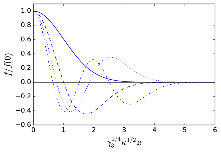
Figure 1: Fundamental (continuous) and first three excited (dashed for $m=1$, dotted for $m=2$, and dot-dashed for $m=3$) solutions in the limit $\xi\gg 1$.

This approximation is valid provided all nodes are well inside the interior region, i.e., $m\ll\xi/4$. We thus expect that solutions with $m$ nodes exist up to a maximum value $m_{\mathrm{max}}$ close to $\xi/4$. One can also estimate the positions of the roots using the explicit form of the Laguerre polynomials. For instance, for the first excited solution, we find that the unique root is at

$$x_{0}\approx\left(\gamma_{3}\kappa^{2}\right)^{-1/4},$$ (43)

while for the second excited solution, the two roots are at $x_{0}\approx\left[(2\pm\sqrt{2})/\sqrt{\gamma_{3}\kappa^{2}}\right]^{-1/2}$.

We solved Eq. (41) numerically for various values of $\xi$ and found few deviations from the above picture. In particular, solutions with $m$ nodes exist for $m$ between $0$ and a maximum value $m_{\mathrm{max}}$, approximately equal to $\xi/4$ when $\xi\gg 1$. We also solved Eq. (25) numerically using a shooting method to see the effects of the nonlinear term as well as that of a more realistic profile for $h$. Concerning the former, we found its main effect is to decrease the value of $\mu$ of each solution, by a term quadratic in $f(0)$. For each value of $m$, there is a critical value of $\left\lvert f(0)\right\rvert$ above which the solution disappears as the corresponding value of $\mu$ drops below $-1$, as shown in Fig. 2 for the fundamental solution with $\xi=4$. The nonlinear term also has the tendency to widen the condensate, although this becomes significant only close to the critical value.

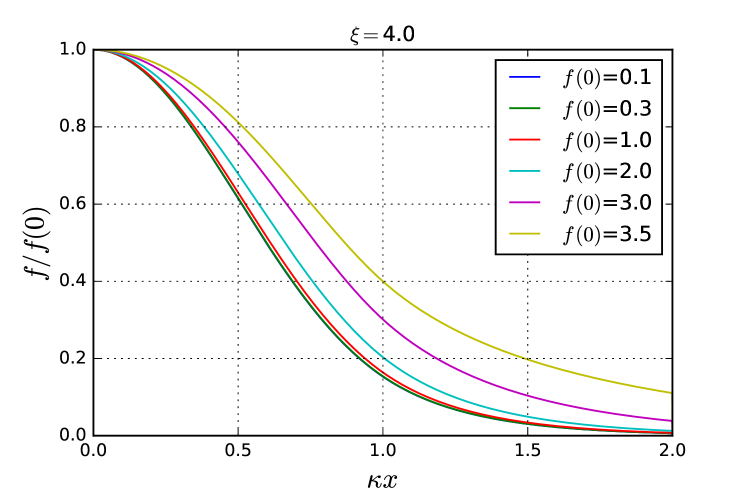
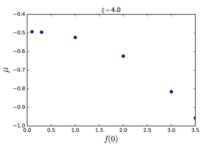
Figure 2: Top panel: Fundamental solutions for $\xi=4$ and different values of $f(0)$, expressed in units of $\kappa/\sqrt{\gamma_{2}}$. Bottom panel: Values of the parameter $\mu$ for these solutions.

Similarly, we found that replacing the above profile of $h$ with a hyperbolic tangent does not change the qualitative behavior of the solutions. Its main effect is to increase $m_{\mathrm{max}}$, which seems to come from the slower convergence of $h$ towards $1$.

III.2 Numerical construction

We have solved numerically the coupled set of differential equations (9), (11) and (12), subject to the appropriate boundary conditions (13) and (14).

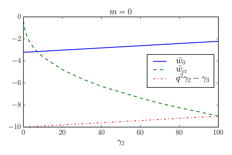
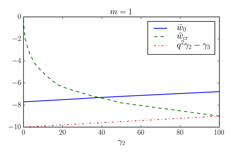
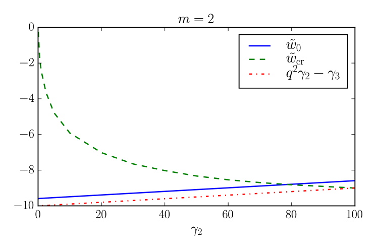
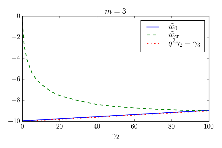
Figure 3: The value of $\tilde{w}_{\mathrm{cr}}$ and $\tilde{w}_{0}$ in dependence on $\gamma_{2}$ for $q=0.1$, $\gamma_{3}=10$, $\alpha_{1}=0.01$ and $m=0,1,2,3$ (top to bottom), respectively. We also give the negative value of the effective mass of the condensate function, $-m_{\sigma}^{2}=q^{2}\gamma_{2}-\gamma_{3}$.

III.2.1 A case study

In what follows, we concentrate on the solutions for $q=0.1$, $\alpha_{1}=0.01$ and $\gamma_{3}=10$ and study the effects of the variation of $\gamma_{2}$. This case is complementary to the study done in Hartmann et al. (2017), where the couplings $\gamma_{2}$ and $\gamma_{3}$ had been chosen one to two orders of magnitude larger. First let us recall that restrictions on the couplings exist in this model, in particular we have $\gamma_{2}\leq\gamma_{3}^{2}$, such that in the following we will study solutions for $\gamma_{2}\in]0:100[$. Note that the second requirement $q^{4}\gamma_{2}^{2}\leq\gamma_{2}$ is automatically fulfilled within this interval of the parameter $\gamma_{2}$.

We have constructed solutions with up to 3 nodes in the condensate field function. We observe that for all values of $m$ solutions exist in a limited interval of the central value of the condensate field, $f(0)\in[0:f(0)_{\mathrm{max}}]$ such that for $f(0)\rightarrow 0$ the field function $f(x)\equiv 0$. This corresponds to a value of the state parameter $\tilde{w}$ which we will denote $\tilde{w}_{0,m}$ in the following. Our results for $m=0,1,2,3$ are shown in Fig. 3. In all plots, we show the (negative) value of the effective mass of the condensate field, which is given by $m_{\sigma}^{2}=\gamma_{3}-q^{2}\gamma_{2}$. We observe that $\tilde{w}_{0,m}$ is a linear function of $\gamma_{2}$ and is parallel to $-\tilde{m}_{\sigma}^{2}$ for all values of $m$. The difference $\Delta_{m}:=\tilde{w}_{0,m}-(-\tilde{m}_{\sigma}^{2})$ decreases with increasing node number $m$. The values are given in Table 1. For the given parameter values, we hence find that the formula

$$\tilde{w}_{0,m}=\Delta_{m}-\gamma_{3}+q^{2}\gamma_{2}$$

holds.

Our numerical results indicate that $f(0)$ can be increased up to a maximal value $f(0)_{\mathrm{max}}$ which depends on the values of the couplings in the model. We will denote the corresponding value of the state parameter $\tilde{w}_{\mathrm{cr},m}$ in the following. The value of $\tilde{w}_{\mathrm{cr},m}$ is a decreasing function of $\gamma_{2}$. The qualitative behaviour is similar for all values of $m$ : $\tilde{w}_{\mathrm{cr},m}=0$ for $\gamma_{2}\rightarrow 0$ and decreases to $\tilde{w}_{\mathrm{cr},m}=-9$ for $\gamma_{2}\rightarrow 100$, where it meets with the curve for $-m_{\sigma}^{2}$.

Let us denote the value of $\gamma_{2}$ at which $\tilde{w}_{\mathrm{cr},m}=\tilde{w}_{0,m}$ by $\gamma^{(\mathrm{eq},m)}_{2}$, the numerical values of which are given in Table 1 for $m=0,1,2,3$.

$m$	$\Delta_{m}$	$\gamma_{2}^{(\mathrm{eq},m)}$
$0$	$6.70$	$7$
$1$	$2.20$	$34$
$2$	$0.41$	$80$
$3$	$0.05$	$94$

Table 1: Some characteristic values of the $\tilde{w}_{0,m}$ and $\tilde{w}_{\mathrm{cr},m}$ curves shown in Fig. 3.

For $\gamma_{2}=\gamma_{2}^{(\mathrm{eq},m)}$, the qualitative dependence of $\tilde{w}$ on the central condensate value $f(0)$ changes. For $\gamma_{2}>\gamma_{2}^{(\mathrm{eq},m)}$ the state parameter $\tilde{w}$ decreases for increasing $f(0)$ such that for $\tilde{w}\rightarrow\tilde{w}_{\mathrm{cr},m}$ the value of the condensate $f(0)$ becomes very large and, in fact, as our numerical results indicate, tends to infinity, $f(0)_{\mathrm{max}}\rightarrow\infty$. This case has been studied in detail in Hartmann et al. (2017). Here we present our results for the energy per unit length $\tilde{U}$, the tension $\tilde{T}$ and the current $\tilde{C}$ as functions of the state parameter $\tilde{v}$ for $\alpha=0.01$, $q=0.1$, $\gamma_{2}=99$ and $\gamma_{3}=10$ in Fig.4.

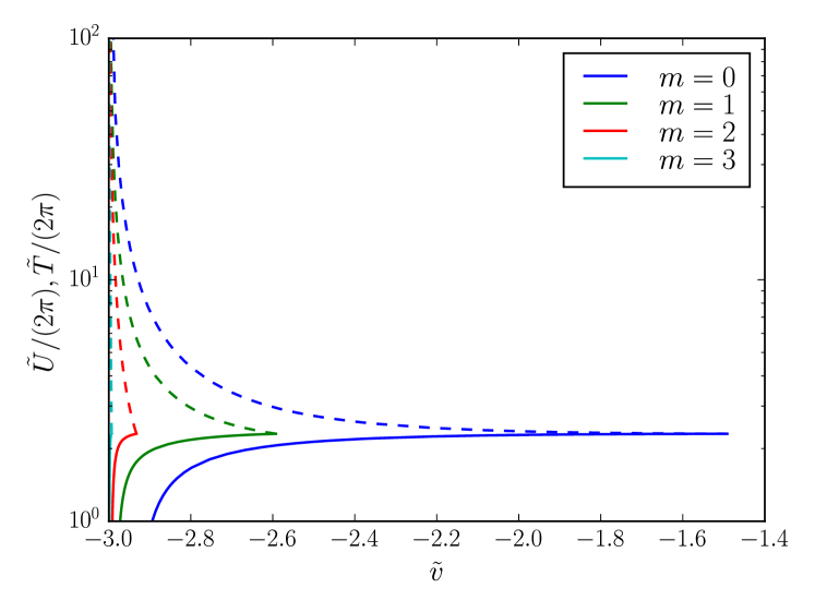
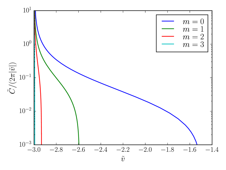
Figure 4: Top : The energy per unit length $\tilde{U}$ (dashed) and the tension $\tilde{T}$ (solid) as function of the state parameter $\tilde{v}$ for $\alpha_{1}=0.01$, $q=0.1$, $\gamma_{2}=99$, $\gamma_{3}=10$ and $m=0,1,2,3$. Bottom : Same as top for the current $\tilde{C}$. The phase frequency threshold of Eq. (26) is clearly visible as the divergence point at $\tilde{w}_{\mathrm{th}}=-\gamma_{3}+q^{2}\gamma_{2}\simeq-3$.

For increasing $m$ the range in $\tilde{v}$, for which superconducting string solutions exist decreases. At $\tilde{v}_{\rm 0}$ the energy per unit length and tension are equal and the current $\tilde{C}$ becomes zero. At $\tilde{v}_{\rm cr}$ the current diverges. We find that independent of the value of $m$, $\tilde{v}_{\rm cr}=-3$ and that the maximal value of $f(0)_{\rm max}$ corresponding to this critical value is (nearly) independent of the node number. Given the interpretation put forward in Carter (1994), namely considering the current $\tilde{C}$ and $\tilde{v}$ as a conjugate pair, in which $|\tilde{v}|$ is the particle number density and $\tilde{C}$ the chemical potential or effective mass per particle, we find that solutions exist only above a certain particle number density, which increases with increasing node number $m$. Furthermore, for a given particle number density $|\tilde{v}|$, the effective mass per particle is largest for the $m=0$ solution and decreases with increasing node number. At the maximal possible particle number $|\tilde{v}_{\rm cr}|$ the current diverges.

For $\gamma_{2}<\gamma_{2}^{(\mathrm{eq},m)}$, on the other hand, we find that $f(0)$ can be increased up to a maximal value $f(0)_{\mathrm{max}}$, which is finite, and that $\tilde{w}$ is an increasing function of $f(0)$. From this maximal value of $f(0)$ a second branch of solutions exists for decreasing $f(0)$, while the state parameter $\tilde{w}$ further increases. We will discuss the origin of the existence of this branch and the physical phenomena associated to it in subsection III.2.3.

III.2.2 Higgs field oscillations

During the study of smaller values of the couplings $\gamma_{2}$ and $\gamma_{3}$, we observed a new phenomenon that is not present for the cases presented in Hartmann et al. (2017). The reason for this is that the central value of the condensate function, $f(0)$ can have larger values for smaller values of $\gamma_{2}$ and $\gamma_{3}$, respectively. For sufficiently large values of $f(0)$ we find that the oscillations of the condensate function can trigger an oscillatory behavior in the Higgs field function. This is shown for $\gamma_{2}=\gamma_{3}=10$, $q=0.1$, $\alpha_{1}=0.01$ and $m=2$ in Fig. 6, in which we also show the condensate field function $f(x)$ together with the Higgs field function $h(x)$ for increasing values of $f(0)$ up to the maximal possible value of $f(0)\approx 0.742$. As can be clearly seen here, the Higgs field function increases monotonically from zero at the origin to unity at infinity for small values of $f(0)$, here $f(0)=0.01$ and $f(0)=0.1$. But as soon as $f(0)$ is large enough, we see that the Higgs field starts to show an oscillating behaviour, see the profiles for $f(0)=0.5$ and $f(0)=0.742$.

For values of $\gamma_{2}$ and $\gamma_{3}$ even smaller – and consequently $f(0)$ much larger – we observe oscillations of the Higgs field with large relative amplitudes on a finite interval of the radial coordinate $x$, on which the Higgs field function possesses nodes. As a first approximation this can be understood by considering (11) and assuming that the terms in $P$ and $h^{3}$ can be neglected with respect to the $f^{2}$ term. Assuming further that the oscillations appear away from the origin $x=0$, we can also neglect (to first approximation) the $h^{\prime}$ term such that the equation reads $h^{\prime\prime}\approx h\left[\gamma_{3}f^{2}(x)-1\right]$, which has oscillating solutions for $\gamma_{3}f^{2}(x)-1<0$. Our numerics confirms this and we find that the Higgs field oscillations occur in an interval of $x$ which is bounded by those two values of $x$ for which $\gamma_{3}f^{2}(x)-1=0$. This is shown in Fig. 5 for $m=2$, $\alpha_{1}=0.01$ $\gamma_{2}=10^{-6}$, $\gamma_{3}=0.01$, $q=0.1$ and $\tilde{w}=-0.007$, i.e. a solution very close to the chiral limit. This solution has central condensate value $f(0)\approx 28.5$ and clearly possesses oscillations of the Higgs field in the two intervals of $x$, where $\gamma_{3}f^{2}(x)-1<0$.

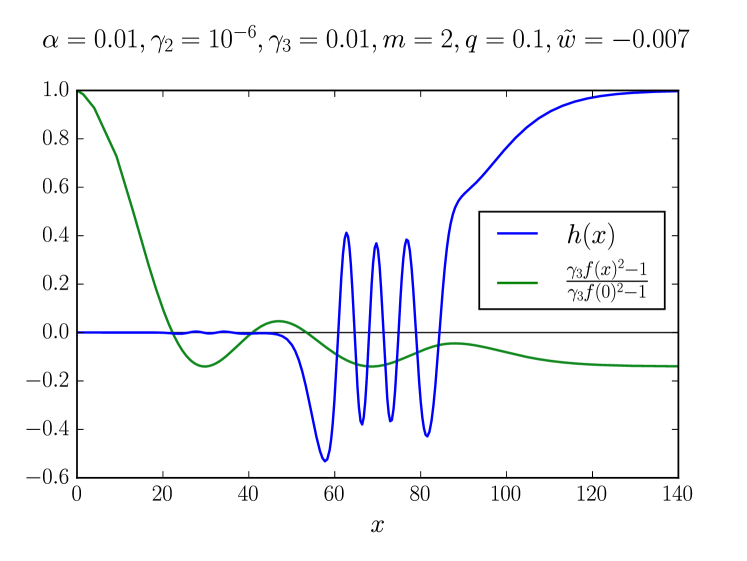
Figure 5: The Higgs field function $h(x)$ together with $\left[\gamma_{3}f^{2}(x)-1\right]/\left[\gamma_{3}f^{2}(0)-1\right]$ for $m=2$, $\alpha_{1}=0.01$, $\gamma_{2}=10^{-6}$, $\gamma_{3}=0.01$, $q=0.1$ and $\tilde{w}=-0.007$.

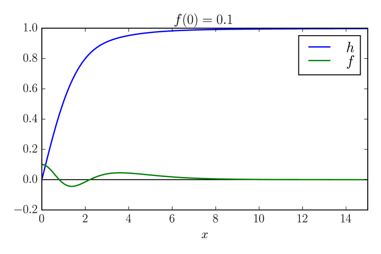
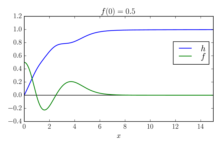
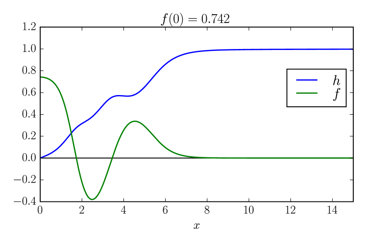
Figure 6: The string-forming Higgs field profile $h(x)$ and the condensate $f(x)$ as functions of the rescaled core radius $x$ for $\alpha_{1}=0.01$, $q=0.1$, $\gamma_{2}=\gamma_{3}=10$, $m=2$ and various values of $f(0)\in\{0.1,0.5,0.742\}$ (from top to bottom).

We have also investigated cases with different values of $m>0$ and $\gamma_{3}$ and confirm that for the parameter range studied here, the back-reaction of the condensate function induces oscillations in the Higgs field function when $f(0)$ becomes large, i.e. when non-linear back-reaction effects can no longer be neglected.

Note that we do not observe oscillations in the limit $f(0)\rightarrow 0$ and/or for $m=0$, hence this phenomenon is restricted to a regime of the parameter space which allows for large values of $f(0)$. We believe this phenomeon to be very rich and to have important implications. A detailed numerical analysis, which is outside the scope of this paper, is hence left as future work.

III.2.3 The second branch

When increasing the central value $f(0)$ of the condensate function we observe that the structure associated to the oscillation of the condensate function remains close to the string axis. This changes on the second branch of solutions mentioned above. Decreasing $f(0)$ from its maximal value, the value of $\tilde{w}$ increases further on the second branch. We observe that, although the value of $f(0)$ decreases, it does so slowly. However, with increasing $\tilde{w}$ the structure associated to the condensate field oscillations moves to larger values of $x$, i.e. we obtain solutions with $h(x)\approx 0$ and $f(x)\approx\mathrm{constant}\lesssim f(0)_{\mathrm{max}}$ on an interval $x\in[0:\delta]$, where $\delta$ increases with increasing $\tilde{w}$. This is shown for $m=2$, $\alpha_{1}=1.0$, $\gamma_{2}=1.0$, $\gamma_{3}=10$, $q=0.1$ and increasing value of $\tilde{w}$ in Fig. 7. For $w=-9.8$ the value of $f(0)=0.1$. Increasing $\tilde{w}$ up to $\tilde{w}_{\mathrm{c}r}=-2.47$ the value of $f(0)$ and with that the condensate and current increase close to the string axis. The maximal possible value of $f(0)$ in this case is $f(0)=f(0)_{\mathrm{m}ax}\approx 1.45$. Increasing $\tilde{w}$ further leads now to the decrease of $f(0)$ and the increase of $\delta$. For $\tilde{w}=-1.2$ and $\tilde{w}=-1.1$, respectively, we find $f(0)=1.1$ and $f(0)=1.05$.

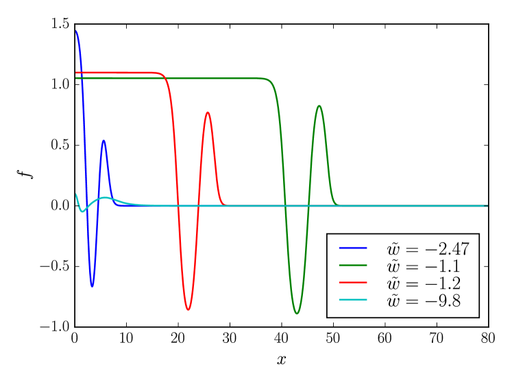
Figure 7: The condensate field function $f(x)$ for $m=2$, $\alpha_{1}=1.0$, $\gamma_{2}=1.0$, $\gamma_{3}=10.0$, $q=0.1$ for increasing values of $\tilde{w}$. Note that $\tilde{w}=-2.47$ corresponds to $\tilde{w}_{\mathrm{cr}}$.

The fact that the structure moves out to infinity can also be clearly seen when investigating the location of the zeros of the condensate function. This is shown for a solution with $m=2$ nodes, $\alpha_{1}=1.0$, $\gamma_{2}=1.0$, $\gamma_{3}=10.0$, $q=0.1$ in Fig. 8, where we give the positions $x_{1}$ and $x_{2}$, respectively, of the two nodes in dependence of $\tilde{w}$.

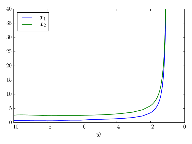
Figure 8: The values $x_{1}$ and $x_{2}$ of the first and second node of the condensate function $f(x)$ in dependence on $\tilde{w}$ for $m=2$, $\alpha_{1}=1.0$, $\gamma_{2}=1.0$, $\gamma_{3}=10.0$ and $q=0.1$.

Decreasing $\tilde{w}$ on the second branch of solutions turns out to be numerically very difficult, but we believe it to be very reasonable that this second branch can be extended backwards all the way to $f(0)=0$, in the limit of which the structures moves to infinity and the energy per unit length $U$ and the tension $T$ tend to infinity. We can understand this dependence by considering the condensate field equation (12) on the interval $x\in]0:\delta]$, where $h(x)\equiv 0$ and $f(x)=\mathrm{constant.}=f(0)$ Excluding the possibility $f(x)\equiv 0$, this implies that $\tilde{w}+\gamma_{2}\left[f(0)^{2}-q^{2}\right]=0$. We demonstrate that our numerical data joins this curve for three different sets of parameters, see Fig. 9. Hence, though the numerics becomes very hard at the end points of the respective numerical data curves, the analytically given curves are (very likely) the proper continuation. We do not see any indications in the numerics that the curves should stop.

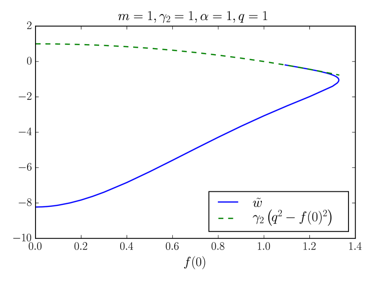
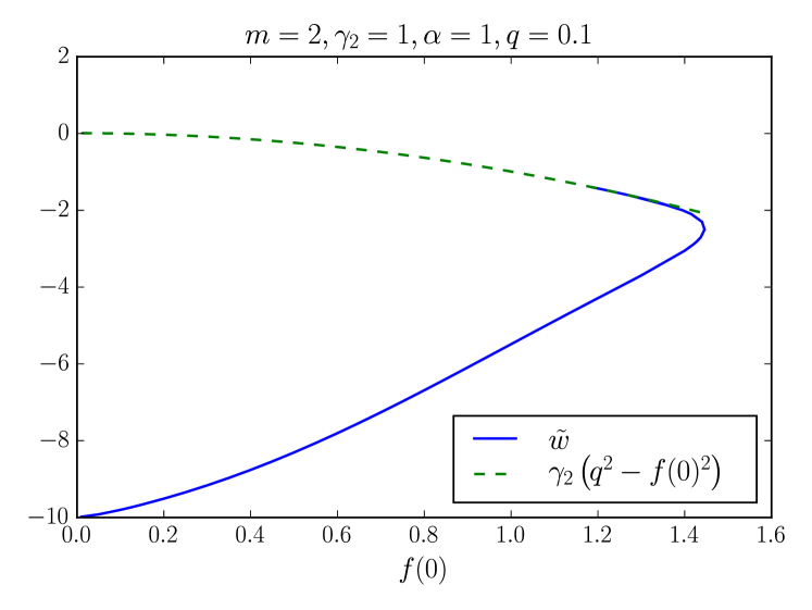
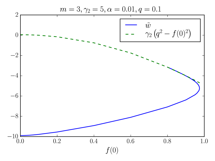
Figure 9: The value of $\tilde{w}$ as function of $f(0)$ for three different sets of parameter choices with $\gamma_{3}=10$. We give the numerical data (solid blue) as well as the analytic curve $\gamma_{2}(q^{2}-f(0)^{2})$ (dashed green).

Finally, let us explain qualitatively why two branches of solutions in $f(0)$ exist in our model. This is easily understood when remembering that we have rescaled the radial coordinate $r\rightarrow x=r/\Lambda$ as well as the state parameter $w\rightarrow\tilde{w}=\Lambda^{2}w$, where $\Lambda=(\sqrt{\lambda_{1}}\eta_{1})^{-1}$ is the length scale associated to the Higgs field. When increasing $\tilde{w}$ on the first branch of solutions, we increase the condensate close to the string axis until we reach the maximal possible value of the condensate related to a value of $\tilde{w}$, which stays fixed on the second branch of solutions and is negative in the case studied above. Now to increase the value of $\tilde{w}$ further, i.e. make it tend to zero from below, we need to decrease $\Lambda$. But this in turn implies that the rescaled radial coordinate $x$ increases. This is exactly what we observe in our numerics – the non-trivial structure in the fields moves out to larger values of $x$.

III.2.4 Strings with $n>1$

We have also constructed superconducting string solutions with $n>1$, motivated by a recent study done in a very similar model Forgacs and Lukács (2016); Forgács and Lukács (2016). As our stability analysis below shows, the qualitative behaviour of our results is independent of $n$. To demonstrate this, we have constructed numerically solutions with $n=2$ and $n=3$ and compared these to the $n=1$ case.

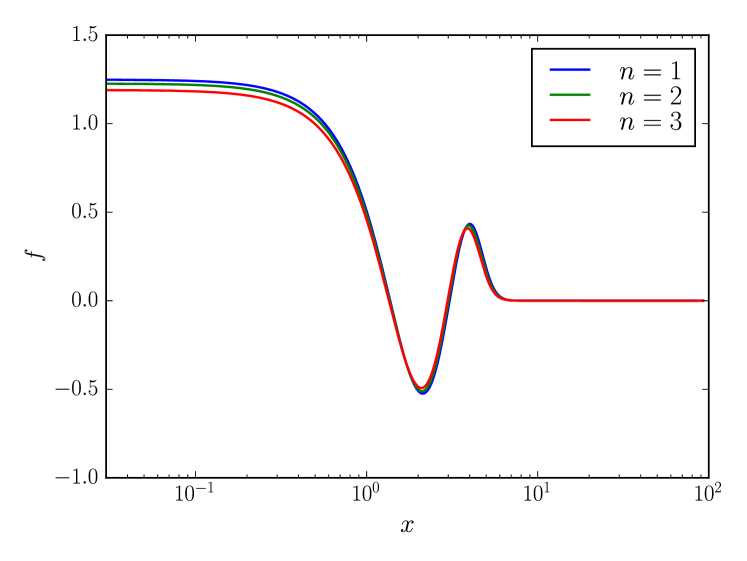
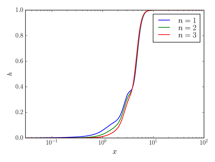
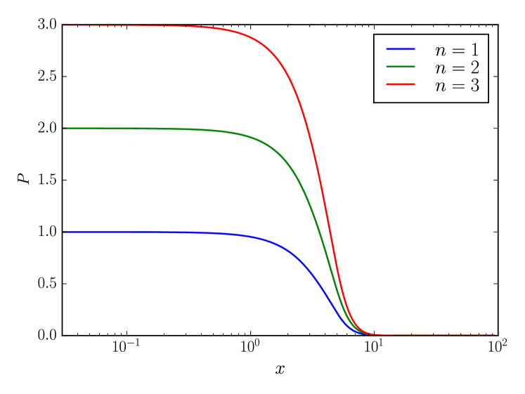
Figure 10: The profiles of the condensate, Higgs and gauge field functions (from top to bottom) for $m=2$, $\alpha_{1}=1$, $\gamma_{2}=1$, $\gamma_{3}=10$, $q=0.1$, $\tilde{w}=-4$ and winding $n=1,2,3$.

Our results for a solution with $m=2$, $\alpha_{1}=1$, $\gamma_{2}=1$, $\gamma_{3}=10$, $q=0.1$, $\tilde{w}=-4$ are shown in Fig. 10. The condensate function $f(x)$ is practically unchanged, although we observe a small decrease in the central value $f(0)$ with increasing $n$ (see Table II for the numerical values). Moreover, the oscillations in the Higgs field function $h(x)$ that we observed for $n=1$ persist for $n=2,3$, although slightly modified. As far as the integrated quantities are concerned, we observe that the energy per unit length $\tilde{U}$ per winding $n$, i.e. $\tilde{U}/n$ slightly decreases indicating that for our choice of couplings a superconducting string with higher $n$ can be interpreted as a bound state of $n$ superconducting strings with winding $n=1$. The numerical values of $\tilde{U}/n$ as well as $\tilde{T}/n$ are given in Table II. This relates to the observations made in Forgacs and Lukács (2016); Forgács and Lukács (2016). Finally, let us mention that we also find that the value of the current $\tilde{C}$ decreases with increasing $n$. A more detailed analysis of this fact is out of the scope of this paper and is left as future work.

$n$	$f(0)$	$\displaystyle\frac{\tilde{T}}{2\pi n}$	$\displaystyle\frac{\tilde{U}}{2\pi n}$	$\displaystyle\frac{\tilde{C}}{2\pi|\tilde{v}|}$
$1$	$1.245$	$0.314$	$7.679$	$1.841$
$2$	$1.227$	$0.234$	$3.672$	$1.719$
$3$	$1.190$	$0.234$	$2.311$	$1.558$

Table 2: Comparison of some characteristic values of solutions with different windings (see also Fig. 10).

III.3 Carter stability

The macroscopic stability criterion of superconducting strings Carter (1989) relates the velocities of longitudinal and transversal perturbations to the energy per unit length $U$ and the tension $T$. In the neutral limit $e_{2}\to 0$, the definitions above imply that all the integrated quantities $U$, $T$ and $C$ are positive definite. One also finds, from the definitions, the useful relationship

$$U-T=|v|C\ \ \ \Longleftrightarrow\ \ \ \ \tilde{U}-\tilde{T}=|\tilde{v}|\tilde{C},$$ (44)

from which one can prove Peter (1992a) that there exists a finite neighborhood around $v=0$ for which the string is macroscopically stable, i.e. both the transverse ($c_{\mathrm{{}_{T}}}$) and the longitudinal ($c_{\mathrm{{}_{L}}}$) velocities, defined above, are real. Indeed, let us first consider the spacelike case for which $v\geq 0$. In that case, the energy per unit length happens to equal the Lagrangian from which one deduces the field equations (9) to (12), so that differentiating $U$ with respect to $v$ reduces merely to differentiating the explicit appearance of $v$. Looking at Eq. (16), one sees that this amounts to

$$v\geq 0:\ \ \ \ \ \frac{\mathrm{d}U}{\mathrm{d}v}=C\ \ \ \ \underset{\eqref{UTC}}{\Longrightarrow}\ \ \ \ \frac{\mathrm{d}T}{\mathrm{d}v}=-v\frac{\mathrm{d}C}{\mathrm{d}v}.$$ (45)

Similarly, for $v\leq 0$, the Lagrangian yielding the field equations now being $T$, one obtains,

$$v\leq 0:\ \ \ \ \ \frac{\mathrm{d}T}{\mathrm{d}v}=C\ \ \ \ \underset{\eqref{UTC}}{\Longrightarrow}\ \ \ \ \frac{\mathrm{d}U}{\mathrm{d}v}=-v\frac{\mathrm{d}C}{\mathrm{d}v}.$$ (46)

We noted earlier that $C\geq 0$, and given its definition (24), it is clear that $\lim_{v\to 0}C=0$: this implies that for $v\geq 0$, there exists a finite neighborhood around $v=0$ such that $\mathrm{d}C/\mathrm{d}v\geq 0$. In this region, the first equality in Eq. (45) ensures that $\mathrm{d}T/\mathrm{d}v\leq 0$, which, combined with the second one stating that $\mathrm{d}U/\mathrm{d}v\geq 0$, implies that $c_{\mathrm{{}_{L}}}^{2}\geq 0$. Reverting a few signs and using (46) for $v\leq 0$ shows the same conclusion holds in a finite neighborhood for negative $v$. These arguments depending only on the definition of the integrated quantities and on the equations of motion that are satisfied by the fields together with the boundary conditions, show that there must exist a finite region of state parameter in which the ground state and the excited configurations are Carter stable for both electric (timelike) and magnetic (spacelike) currents.

In the region of parameter space studied in Sec. III.2 however, the condensate exists only for strictly negative values of the state parameter, and therefore the argument cannot apply, although it does apply in many other regimes, such as that discussed in Ref. Hartmann et al. (2017). Here, one must resort to the numerical solution, such as that shown in Fig. 4. We see that Carter criterion for stability is indeed fulfilled, so it would appear our modes are macroscopically stable. We must therefore now move on to a local analysis to show the microscopic instability leading to the cosmological consequences drawn in Ref. Hartmann et al. (2017) and further elaborated in our concluding section V.

III.4 Linear stability analysis and decay rate

To determine the possible physical effects of the excited solutions, a crucial piece of information is whether they are stable – and, if not, what is the typical time scale of their decay. While a full stability analysis is beyond the scope of the present paper, useful information can be obtained from the study of linear perturbations, on which we now concentrate. As we wish to determine the evolution in time of the solutions after small perturbations, we need the field equations for $t$- and $z$-dependent fields. For simplicity, we consider only those solutions where $\sigma$ and $B_{\mu}$ are independent on $\theta$. The field equations are

$$\partial_{t}^{2}\sigma-\partial_{z}^{2}\sigma-\partial_{r}^{2}\sigma-\frac{1}{r}\nobreak\hskip 0.80002pt\partial_{r}\sigma+2\nobreak\hskip 0.80002pt\partial_{\sigma^{*}}V=0,$$ (47)

$$\left(\partial_{t}-\mathrm{i}\nobreak\hskip 0.80002pte\nobreak\hskip 0.80002ptB_{t}\right)^{2}\phi-\left(\partial_{z}-\mathrm{i}\nobreak\hskip 0.80002pte\nobreak\hskip 0.80002ptB_{z}\right)^{2}\phi-\left(\partial_{r}-\mathrm{i}\nobreak\hskip 0.80002pte\nobreak\hskip 0.80002ptB_{r}\right)^{2}\phi-\frac{1}{r^{2}}\nobreak\hskip 0.80002pt\left(\partial_{\theta}-\mathrm{i}\nobreak\hskip 0.80002pte\nobreak\hskip 0.80002ptB_{\theta}\right)^{2}\phi-\frac{1}{r}\nobreak\hskip 0.80002pt\left(\partial_{r}-\mathrm{i}\nobreak\hskip 0.80002pte\nobreak\hskip 0.80002ptB_{r}\right)\phi+2\partial_{\phi^{*}}V=0,$$ (48)

$$\partial_{\nu}\partial^{\nu}B_{t}-\frac{1}{r}\nobreak\hskip 0.80002pt\partial_{r}B_{t}-\partial_{t}\left(\partial_{\nu}B^{\nu}-\frac{1}{r}\nobreak\hskip 0.80002ptB_{r}\right)+\mathrm{i}\nobreak\hskip 0.80002pt\frac{e}{2}\nobreak\hskip 0.80002pt\left[\phi^{*}\nobreak\hskip 0.80002pt\left(\partial_{t}-\mathrm{i}\nobreak\hskip 0.80002pte\nobreak\hskip 0.80002ptB_{t}\right)\phi-\phi\nobreak\hskip 0.80002pt\left(\partial_{t}+\mathrm{i}\nobreak\hskip 0.80002pte\nobreak\hskip 0.80002ptB_{0}\right)\phi^{*}\right]=0,$$ (49)

$$\partial_{\nu}\partial^{\nu}B_{z}-\frac{1}{r}\nobreak\hskip 0.80002pt\partial_{r}B_{z}-\partial_{z}\left(\partial_{\nu}B^{\nu}-\frac{1}{r}\nobreak\hskip 0.80002ptB_{r}\right)+\mathrm{i}\nobreak\hskip 0.80002pt\frac{e}{2}\nobreak\hskip 0.80002pt\left[\phi^{*}\nobreak\hskip 0.80002pt\left(\partial_{z}-\mathrm{i}\nobreak\hskip 0.80002pte\nobreak\hskip 0.80002ptB_{z}\right)\phi-\phi\nobreak\hskip 0.80002pt\left(\partial_{z}+\mathrm{i}\nobreak\hskip 0.80002pte\nobreak\hskip 0.80002ptB_{z}\right)\phi^{*}\right]=0,$$ (50)

and

$$\partial_{\nu}\partial^{\nu}B_{r}+\frac{2}{r^{3}}\nobreak\hskip 0.80002pt\partial_{\theta}B_{\theta}-\partial_{r}\partial_{\nu}B^{\nu}+\mathrm{i}\nobreak\hskip 0.80002pt\frac{e}{2}\nobreak\hskip 0.80002pt\left[\phi^{*}\nobreak\hskip 0.80002pt\left(\partial_{r}-\mathrm{i}\nobreak\hskip 0.80002pte\nobreak\hskip 0.80002ptB_{r}\right)\phi-\phi\nobreak\hskip 0.80002pt\left(\partial_{r}+\mathrm{i}\nobreak\hskip 0.80002pte\nobreak\hskip 0.80002ptB_{r}\right)\phi^{*}\right]=0.$$ (51)

In the following, in order to keep the equations as simple as possible, we assume $\phi^{*}\nobreak\hskip 0.80002pt\partial_{\mu}\phi\in\mathbb{R}$ for $\mu\neq\theta$.

Let us assume we have a solution $\phi=\phi^{(0)}$, $\sigma=\sigma^{(0)}$, $B_{\mu}=B_{\mu}^{(0)}$ of the form given in Eqs. (5) and (6). We look for perturbed solutions of the form $\phi=\phi^{(0)}+\delta\phi$, $\sigma=\sigma^{(0)}+\delta\sigma$, $B_{\mu}=B_{\mu}^{(0)}+\delta B_{\mu}$, where

$$\delta\phi(t,r,\theta,z) =p(r)\exp\left[\mathrm{i}\nobreak\hskip 0.80002pt\left(n\nobreak\hskip 0.80002pt\theta+\sqrt{\lambda_{1}}\nobreak\hskip 0.80002pt\eta_{1}\nobreak\hskip 0.80002pt\nu\nobreak\hskip 0.80002ptt-\sqrt{\lambda_{1}}\nobreak\hskip 0.80002pt\eta_{1}\nobreak\hskip 0.80002pt\kappa\nobreak\hskip 0.80002ptz\right)\right]\nobreak\hskip 0.80002pt,$$

$$\delta\sigma(t,r,\theta,z) =s(r)\exp\left\{\mathrm{i}\nobreak\hskip 0.80002pt\left[(\omega+\sqrt{\lambda_{1}}\nobreak\hskip 0.80002pt\eta_{1}\nobreak\hskip 0.80002pt\nu)\nobreak\hskip 0.80002ptt-(k+\sqrt{\lambda_{1}}\nobreak\hskip 0.80002pt\eta_{1}\nobreak\hskip 0.80002pt\kappa)\nobreak\hskip 0.80002ptz\right]\right\}\nobreak\hskip 0.80002pt,$$

$$\delta B_{\theta}(t,r,\theta,z) =a(r)\exp\left[\mathrm{i}\nobreak\hskip 0.80002pt\left(\sqrt{\lambda_{1}}\nobreak\hskip 0.80002pt\eta_{1}\nobreak\hskip 0.80002pt\nu\nobreak\hskip 0.80002ptt-\sqrt{\lambda_{1}}\nobreak\hskip 0.80002pt\eta_{1}\nobreak\hskip 0.80002pt\kappa\nobreak\hskip 0.80002ptz\right)\right]\nobreak\hskip 0.80002pt,$$ (52)

$(\nu,\kappa)\in\left(\mathrm{i}\nobreak\hskip 0.80002pt\mathbb{R}\right)^{2}$, and $a$, $p$, $s$ are three real-valued functions. We work in the gauge $\partial_{\mu}\delta B^{\mu}=0$ and assume $B_{r}=B_{t}=B_{z}=0$. One can easily show that the resulting system of equations is self-consistent provided the algebraic relation $\omega\nobreak\hskip 0.80002pt\nu=k\nobreak\hskip 0.80002pt\kappa$ is satisfied. When allowing $\nu$ and/or $\kappa$ to be more general complex numbers, $B_{r}$, $B_{t}$ and $B_{z}$ are sourced by the imaginary part of $\phi^{*}\nobreak\hskip 0.80002pt\partial_{\mu}\phi$ and can thus not be set to zero, which is why we restrict attention to perturbation satisfying $\Im\mathrm{m}\left(\phi^{*}\nobreak\hskip 0.80002pt\partial_{\mu}\phi\right)=0$.

The system to be solved is then

$$\left\{\begin{aligned} &\frac{1}{x}\nobreak\hskip 0.80002pt\partial_{x}\left(x\nobreak\hskip 0.80002pt\partial_{x}s\right)=\left(\tilde{w}+\kappa^{2}-\nu^{2}+3\nobreak\hskip 0.80002pt\gamma_{2}\nobreak\hskip 0.80002ptf^{2}-\gamma_{2}\nobreak\hskip 0.80002ptq^{2}+\gamma_{3}\nobreak\hskip 0.80002pth^{2}\right)\nobreak\hskip 0.80002pts+2\nobreak\hskip 0.80002pt\gamma_{3}\nobreak\hskip 0.80002ptf\nobreak\hskip 0.80002pth\nobreak\hskip 0.80002ptp,\\ &\frac{1}{x}\nobreak\hskip 0.80002pt\partial_{x}\left(x\nobreak\hskip 0.80002pt\partial_{x}p\right)=\left(-\nu^{2}+\kappa^{2}+\frac{P^{2}}{r^{2}}+3\nobreak\hskip 0.80002pth^{2}-1+\gamma_{3}\nobreak\hskip 0.80002ptf^{2}\right)p+2\nobreak\hskip 0.80002pt\gamma_{3}\nobreak\hskip 0.80002pth\nobreak\hskip 0.80002ptf\nobreak\hskip 0.80002pts-\frac{h\nobreak\hskip 0.80002ptP}{x^{2}}\nobreak\hskip 0.80002pta,\\ &x\nobreak\hskip 0.80002pt\partial_{x}\left(\frac{1}{x}\nobreak\hskip 0.80002pt\partial_{x}a\right)=\left(-\nu^{2}+\kappa^{2}+\alpha^{2}\nobreak\hskip 0.80002pth^{2}\right)a-\alpha^{2}\nobreak\hskip 0.80002ptP\nobreak\hskip 0.80002pth\nobreak\hskip 0.80002pt\left(p+p_{v}\right),\end{aligned}\right.$$ (53)

with the boundary conditions $p(0)=s^{\prime}(0)=a(0)=0$ and $p(\infty)=s(\infty)=a(\infty)=0$. If there exists $\nu\in\mathrm{i}\nobreak\hskip 0.80002pt\mathbb{R}_{-}$ such that this system has a solution, then the background solution is linearly unstable in the sense that it supports perturbations growing exponentially in time. Finding numerical solutions to this system is challenging, as its exponentially-growing solutions make it difficult to reach a satisfactory numerical precision for the bounded ones we are interested in. However, as explained in Appendix A, one can already obtain information about the linear stability of the solution by viewing the Higgs and gauge fields as nondynamical in the linear analysis, i.e., setting $p=a=0$. The system (53) then reduces to

$$\frac{1}{x}\nobreak\hskip 0.80002pt\partial_{x}\left(x\nobreak\hskip 0.80002pt\partial_{x}s\right)=\left(\tilde{w}+\kappa^{2}-\nu^{2}+3\nobreak\hskip 0.80002pt\gamma_{2}\nobreak\hskip 0.80002ptf^{2}-\gamma_{2}\nobreak\hskip 0.80002ptq^{2}+\gamma_{3}\nobreak\hskip 0.80002pth^{2}\right)\nobreak\hskip 0.80002pts.$$ (54)

In the present work, since our main aim is to study the nonlinear solutions rather than linear perturbations we shall work only with Eq. (54). A more general stability analysis may be interesting, but is outside of the scope of the present study; besides, as we also argue below, since the system exhibits instabilities already for this limited range of perturbation shapes, it can only be shown to be even more unstable than what we obtain here.

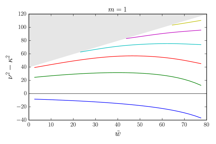
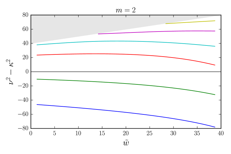
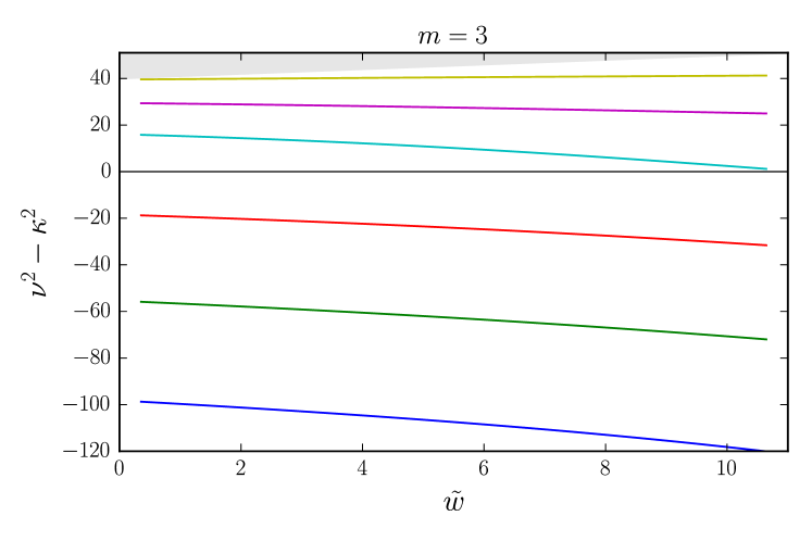
Figure 11: Eigenvalues of Eq. (54) for the solutions with $m=1$ (top), $m=2$ (middle), and $m=3$ (top) nodes in the magnetic case $w>0$. The parameters are $\gamma_{2}=10$, $\gamma_{3}=200$, and $q=4$. The background condensate is computed for a Higgs field $h(x)=\tanh(x)$. The shaded area shows the region $\nu^{2}-\kappa^{2}>w+\gamma_{3}-\gamma_{2}\nobreak\hskip 0.80002ptq^{2}$, in which the modes oscillate at infinity instead of decreasing exponentially. As explained in the text, only negative values of $\nu^{2}-\kappa^{2}$ correspond to instabilities.

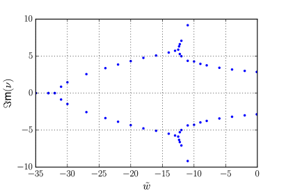
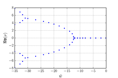
Figure 12: Imaginary (left) and real (right) parts of some modes of the solution with one node in the electric case $w<0$. The parameters are $\gamma_{2}=10$, $\gamma_{3}=200$, and $q=4$. The background condensate is computed for a Higgs field $h(x)=\tanh(x)$.

An instability corresponds to a spatially bounded mode growing exponentially in time (in a given reference frame), i.e., to a bounded solution of Eq. (54) with $\nu^{2}-\kappa^{2}<0$. Since the above derivation requires $\omega\nobreak\hskip 0.80002pt\nu=k\nobreak\hskip 0.80002pt\kappa$, such solutions make sense only for the magnetic case $w>0$. We shall motivate below that the unstable character of the solutions persists in the case $w<0$. Fig. 11 shows the eigenvalues $\nu^{2}-\kappa^{2}$ of Eq. (54) for $\gamma_{2}=10$, $\gamma_{3}=200$, and $q=4$, for the condensates with one, two, and three nodes computed in a fixed Higgs field background $h(x)=\tanh(x)$. Although only the solutions with $\nu^{2}-\kappa^{2}<0$ yield instabilities, we also show those with positive values of this quantity to better illustrate what happens when adding a node to the condensate. The main lessons are the following:

• For $\nu^{2}-\kappa^{2}>\tilde{w}+\gamma_{3}-\gamma_{2}\nobreak\hskip 0.80002ptq^{2}$, the solutions oscillate in the large $x$ region, with an amplitude decaying as $x^{-1/2}$. Bounded solutions thus always exist, providing the continuous spectrum of Eq. (54).

• For $\nu^{2}-\kappa^{2}<\tilde{w}+\gamma_{3}-\gamma_{2}\nobreak\hskip 0.80002ptq^{2}$, the solutions are exponentially increasing or decreasing at infinity. When imposing the boundary condition $s^{\prime}(0)=0$, they are thus spatially bounded only for a discrete set of values of $\nu^{2}-\kappa^{2}$, and represent the discrete spectrum of Eq. (54).

• Among these discrete eigenvalues, one, two, and three are negative for the solutions with one, two, and three nodes, respectively.

The third point is the most important one: it means that the solution with $m$ nodes (for these parameters, and $m$ ranging from $1$ to $3$) has $m$ unstable modes. This property happens to be satisfied for all the sets of parameters we tried numerically. We also verified it holds when working with the actual profile of the Higgs field [solving Eqs. (9) – (12)] instead of the hyperbolic tangent ansatz. We found no instability for the solutions with $m=0$.

As mentioned above, the electric case $w<0$ is more difficult as the above simplification does not apply . However, since the solutions we found are smooth in the limit $w\to 0^{+}$, we conjecture that the aforementioned instabilities will still be present, at least for small values of $-w$. To further motivate this, we show in Fig 12 eigenvalues obtained for the condensate with one node, for the same parameters as in Fig. 11. To obtain them, we can no longer make the assumption $\omega\nobreak\hskip 0.80002pt\nu=k\nobreak\hskip 0.80002pt\kappa$ and Eq. (54) becomes

$$\left[\tilde{w}+\gamma_{2}\nobreak\hskip 0.80002pt\left(2\nobreak\hskip 0.80002ptf^{2}-q^{2}\right)+\gamma_{3}\nobreak\hskip 0.80002pth^{2}-\nu^{2}+\kappa^{2}-2\nobreak\hskip 0.80002pt\left(\tilde{\omega}\nobreak\hskip 0.80002pt\nu-\tilde{k}\nobreak\hskip 0.80002pt\kappa\right)\vphantom{\frac{1}{x}}\right.$$ (55)

$$\left.-\frac{1}{x}\cdot\partial_{x}\cdot x\cdot\partial_{x}\right]s+\gamma_{2}\nobreak\hskip 0.80002ptf^{2}\nobreak\hskip 0.80002pts^{*}=0.$$

We work in a frame where $\tilde{k}=0$ and look for solutions with $\kappa=0$. Notice that the spectrum is invariant under complex conjugation because Eq. (55) is unchanged under $s\to s^{*}$, $\nu\to\nu^{*}$. It is also invariant as well as under the symmetry transformation $(\tilde{\omega},\nu)\to(-\tilde{\omega},-\nu)$. As shown in Fig. 12, at least one eigenvalue with a negative imaginary part is present in most of the domain of $w$ for which the solution with one node exists. Although the argument of Appendix A does not apply to this case, this suggests that these solutions are also unstable. This completes the argument that excited current-carrying cosmic strings are unstable.

Although we are mostly interested in the case where the winding number $n$ is equal to $1$, one may wonder if and how choosing a larger value would affect these results. At the level of the Higgs field, the main difference lies in the behaviour close to the string axis where $h(x)$ is proportional to $x^{n}$. To get a first idea of the structure of the set of solutions for $n>1$, we thus solved Eq. (25) numerically in a background field given by

$$h(x)=\tanh(\kappa\nobreak\hskip 0.80002ptx)^{n},$$ (56)

for $n$ from $2$ and $3$, for the same parameters as in Fig. 12 and with $w=1$. We obtained similar results: first, one solution with $m$ nodes exists for $m$ between $0$ and a maximum value (equal to $4$ for $n=2$ and $5$ for $n=3$); second, the solution with $m$ nodes has $m$ unstable modes. We thus conjecture that the results obtained in this work, concerning both the structure of excited solutions and stability, remain qualitatively valid for $n>1$, as is also confirmed by our numerical construction, shown in III.2.4. A systematic analysis of this case is left for a future work.

IV Electromagnetic and gravitational effects

IV.1 Solutions in the U(1)${}_{\rm gauge}\times$ U(1)_gauge model

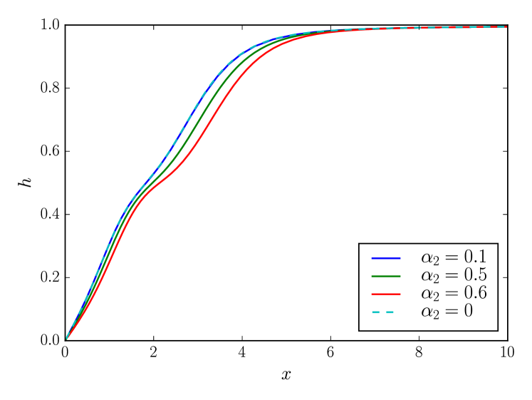
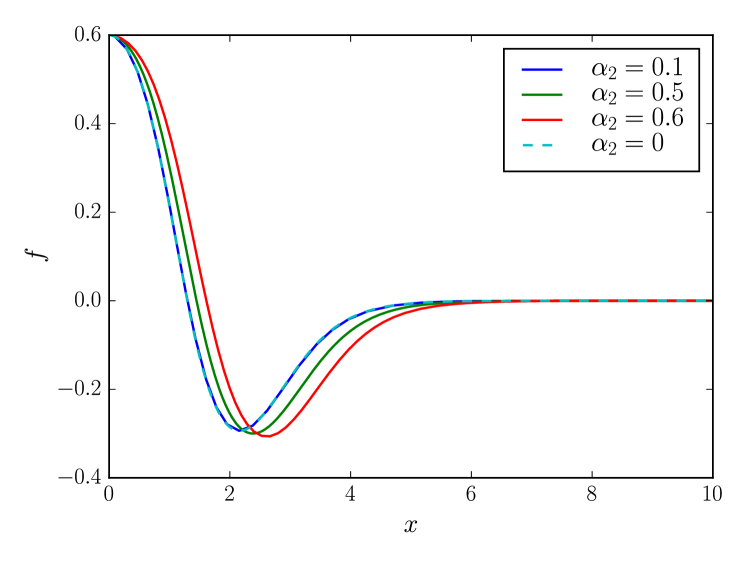
Figure 13: Profiles for the string-forming Higgs field $h(x)$ (top panel), the gauge condensate $f(x)$ (middle) and the asymptotically logarithmic behaving gauge potential $b(r)-1$ (bottom) for an oscillating radially excited solution. The different curves correspond to different values of the rescaled electromagnetic-like coupling constant $\alpha_{2}$.

In this subsection, we discuss the effects of the coupling of the current to an electromagnetic field. Figure 13 shows the field profiles for various values of $\alpha_{2}$ in the case $m=1$. Similar results were obtained for various values of $m$, showing that, as for the background mode Peter (1992b), the internal structure of the current-carrying cosmic string is essentially not modified by inclusion of electromagnetic effects, the latter being, if anything, only capable of long range interactions on the macroscopic behavior of the strings Peter (1993); Gangui et al. (1998). The figure also shows clearly the expected behavior of the gauge potential sourced by an infinitely long current-carrying string, i.e. $b(r)\sim\ln\left(r/r_{\sigma}\right)$, where $r_{\sigma}\simeq m_{\sigma}^{-1}$, the Compton wavelength of the current carrier $\sigma$, provides an order of magnitude estimate of the electromagnetic radius of the vortex.

IV.2 Gravitational effects

The space-time of a superconducting string possesses a deficit angle $\Delta\sim U+T$, similar to that of a Nambu-Goto string Linet (1989), while locally there exists an attractive force towards the string Moss and Poletti (1987); Peter (1994); Peter and Puy (1993), potentially leading to observable effects Garriga and Peter (1994).

The existence of a deficit angle is responsible for a number of physical effects (for a recent review see Vachaspati et al. (2015)). When the string moves, it creates wakes that could e.g. be observable in the 21cm radiation from hydrogen, while the so-called Kaiser-Stebbins-Gott effect Kaiser and Stebbins (1984) leads to discontinuities in the CMB. Furthermore, the deficit angle would lead to gravitational lensing that is quite distinct from that caused by other spatially extended objects. Finally, so-called kinks and cusps on strings as well as the oscillations of string loops are believed to emit gravitational waves.

In order to discuss gravitational effects, we couple the model (1) minimally to gravity and choose the following parametrization of the metric tensor

$$\mathrm{d}s^{2}=N^{2}(x)\mathrm{d}t^{2}-\mathrm{d}x^{2}-L^{2}(x)\mathrm{d}\theta^{2}-K^{2}(x)\mathrm{d}z^{2}\ .$$ (57)

This model has already been studied in Hartmann and Michel (2012) and we refer the reader for more details to this paper. Let us just remark here that there is an extra dimensionless coupling in the model, which corresponds to the ratio between the symmetry breaking scale $\eta_{1}$ and the Planck mass $M_{\mathrm{Planck}}=G_{\mathrm{N}}^{-1/2}$:

$$\beta=8\pi G_{\mathrm{N}}\eta_{1}^{2},$$ (58)

with $G_{\mathrm{N}}$ the Newton constant.

Given the numerical solutions to the coupled matter and gravity equations, we can read of the deficit angle of the space-time from the behaviour of the metric function $L(x)$:

$$\Delta=2\pi(1-c_{1}),\ \hbox{where}\ \ \ L(x\rightarrow\infty)\rightarrow c_{1}x+c_{2}$$ (59)

where $c_{1}$ and $c_{2}$ are constants that have to be determined numerically.

Solving the coupled matter and Einstein equations numerically we determined the deficit angle for the oscillating string solutions, which is given by the sum of the energy density $U$ and the tension $T$. This is nothing new in comparison to the fundamental string solutions, however, we now have a dicrete set of values of the deficit angle for one fixed set of coupling constants. Hence, measuring the deficit angle, e.g. by gravitational lensing, does not uniquely determine the values of the couplings in the model.

We also observe a new effect that is related to the oscillations of the Higgs field appearing for sufficiently large values $f(0)$. We find that these trigger an oscillation in the local scalar curvature. This is demonstrated in Fig. 14 for a $m=2$ solution and various values of the condensate.

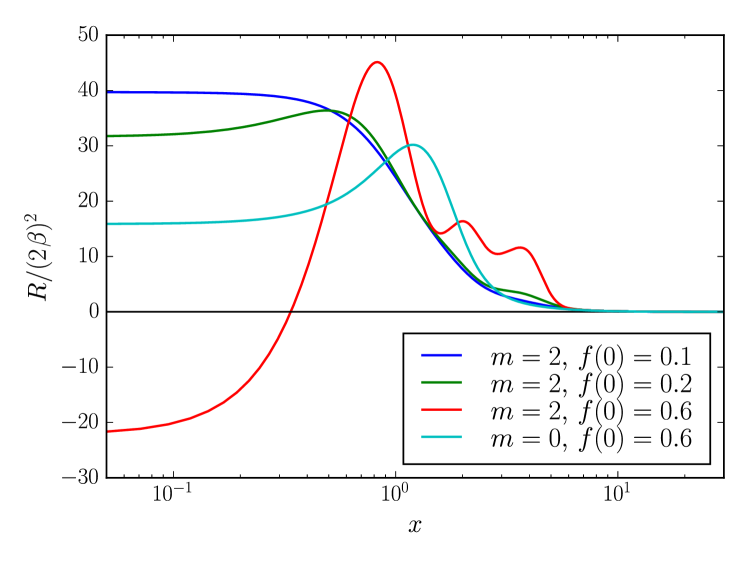
Figure 14: Ricci scalar as a function of string core distance for an $m=2$ oscillatory mode with various values of the condensate interior value $f(0)$.

V Conclusions

In this paper, we have studied excited cosmic string solutions with superconducting currents. These solutions possess a number of nodes in the condensate field function and can trigger – for sufficiently large condensates – oscillations in the Higgs field function as well as in the local scalar curvature in the space-time around the string. Though some of these solutions are macroscopically, i.e. Carter stable, we show that they are microscopically unstable and would decay rapidly after formation.

In the macroscopic description of cosmic strings, which characterizes them solely in terms of their energy per unit length $U$ and tension $T$, our results are interesting because they imply that for a given set of physical parameters, a discrete number of cosmic strings with different values of $U$ and $T$ exist. Assuming that at the formation of cosmic string networks in the primordial universe these excited solutions can be formed, the evolution of the network would involve (from a macroscopic point of view) a number of different types of strings, of which some are unstable. Certainly, this will modifiy the dynamics and evolution of string networks and the question arises immediately whether and how these networks reach a scaling solution.

Moreover, the gravitational effects of cosmic strings are determined by the deficit angle in their space-time (which in turn is determined solely by $U$ and $T$), leading to a number of observable effects such as gravitational lensing as well as wakes and the Kaiser-Stebbins-Gott effect. Now since strings with different values of $U$ and $T$ exist, these will lead to different effects e.g. in the Cosmic Microwave background (CMB) spectra.

From a microscopic point of view, the instability of excited solutions leads to emission of high energy particle radiation that could e.g. be observed in the form of cosmic rays. Moreover, since the local curvature of the space-time around the string is modified by the condensate, it is conceivable that when decaying an additional emission of primordial gravitational waves can be expected.

Finally, let us state that our analysis clearly shows that the underlying field theoretical structure plays a very important role – even when considering only the macrophysics and, hence, integrated quantities. For Nambu–Goto simulations of cosmic string network evolution (see e.g. Bennett and Bouchet (1990, 1989); Blanco-Pillado et al. (2011)) the existence of a network of strings with different tensions and the emission of gravitational waves from excited strings could be of relevance, while for Abelian–Higgs string simulations (see e.g. Vincent et al. (1998); Moore et al. (2002); Hindmarsh et al. (2009) as well as Hindmarsh (2011) and references therein) the excitations of the Higgs field as well as the existence of high energy particle radiation could be interesting to take into account.

Appendix A A note on instabilities

In this appendix we show that, under some conditions, it is possible to study the stability of a field configuration without solving the full set of linearized field equations. More precisely, assuming the field theory has a Hamiltonian structure and the boundary conditions are such that the relevant operator can be diagonalized, we show that finding one unstable mode when viewing all the fields except one   as nondynamical implies that the full theory, with all fields dynamical, also has an instability. Moreover, the growth rate of perturbations in the “restricted” problem with only one dynamical field gives a lower bound on the growth rate of the most unstable mode in the “full” problem. We first focus on the simpler case of a classical particle in two dimensions, which provides some intuition as to why adding one degree of freedom generally does not make a system more stable. We then generalize the results to an arbitrary finite number of dimensions and to field theory. Finally, we explain why they apply to the model dealt with in the main text.

A.1 A toy-model: Classical point particle in a 2D potential

Let us consider a classical particle with mass $m>0$ in a two-dimensional space, subject to a potential $V$. To make things simple, let us assume $V$ is quadratic:

$$V(x,y)=\frac{A}{2}\nobreak\hskip 0.80002ptx^{2}+\frac{B}{2}\nobreak\hskip 0.80002pty^{2}+C\nobreak\hskip 0.80002ptx\nobreak\hskip 0.80002pty,$$ (60)

where $A$, $B$, and $C$ are three real numbers. The equation of motion is

$$m\nobreak\hskip 0.80002pt\partial_{t}^{2}\begin{pmatrix}x\\ y\end{pmatrix}=-\begin{pmatrix}A&C\\ C&B\end{pmatrix}\begin{pmatrix}x\\ y\end{pmatrix}.$$ (61)

To determine the stability of the equilibrium position $x=y=0$, one can look for solutions whith $(x,y)\propto\mathrm{e}^{\mathrm{i}\nobreak\hskip 0.56001pt\nu\nobreak\hskip 0.56001ptt}$ with $\nu\in\mathbb{C}$: the equilibrium is stable if all possible values of $\nu$ are real, and unstable otherwise. Plugging this ansatz into Eq. (61), one finds nontrivial solutions exist if and only if

$$\left\lvert\begin{matrix}A-m\nobreak\hskip 0.80002pt\nu^{2}&C\\ C&B-m\nobreak\hskip 0.80002pt\nu^{2}\end{matrix}\right\rvert=0.$$ (62)

The eigenvalue equation is thus:

$$(A-m\nobreak\hskip 0.80002pt\nu^{2})\nobreak\hskip 0.80002pt(B-m\nobreak\hskip 0.80002pt\nu^{2})-C^{2}=0.$$ (63)

A straightforward calculation gives the possible eigenvalues as

$$\nu^{2}=\frac{(A+B)\pm\sqrt{(A-B)^{2}+4\nobreak\hskip 0.80002ptC^{2}}}{2\nobreak\hskip 0.80002ptm}.$$ (64)

Although it is easy from this expression to determine directly the stability condition, we will here follow a different route which will be easier to generalize to a larger number of degrees of freedom.

This two-dimensional case is very particular in that all eigenvalues can be computed explicitly. However, this is generally not the case in the presence of a large number of degrees of freedom. One possible way to simplify the calculations is to assume some of them are not dynamical. In the present case, for instance, one could set by hand $y=0$ and consider only the stability in the $x$ direction. Then, the equilibrium position will be stable if $A>0$ and unstable if $A<0$. Moreover, in the latter case the growth rate is: $\mathrm{Im}(\nu)=\sqrt{-A/m}$.

Let us now return to Eq. (64) and see what the condition $A<0$ for instability of the “restricted” problem with $y$ set to $0$ by hand can tell us about the stability of the “full” problem where $x$ and $y$ are both dynamical. Taking the $-$ sign in this equation, one gets

$$\nu^{2} =\frac{(A+B)-\sqrt{(A-B)^{2}+4\nobreak\hskip 0.80002ptC^{2}}}{2\nobreak\hskip 0.80002ptm}\leq\frac{(A+B)-(A-B)}{2\nobreak\hskip 0.80002ptm}$$ (65)

$$\nu^{2} \leq\frac{A}{m}.$$

So, the “full” problem also shows an instability, with a growth rate larger than or equal to $\sqrt{-A/m}$. This illustrates a general fact: instabilities obtained when freezing some degrees of freedom give a lower bound on the growth rate of the strongest instability in the “full” problem.

A.2 Generalization to a finite number of degrees of freedom

Let us generalize this to any finite number $N$ of real degrees of freedom. Let $\Phi$ be the vector of perturbations with respect to some equilibrium point. We assume the Lagrangian has the form

$$L=L^{(0)}+\frac{1}{2}\nobreak\hskip 0.80002pt(\partial_{t}\Phi)^{T}\nobreak\hskip 0.80002pt(\partial_{t}\Phi)-\frac{1}{2}\nobreak\hskip 0.80002pt\Phi^{T}\cdot K\cdot\Phi+O(\Phi^{3}),$$ (66)

where $L^{(0)}$ is evaluated at the equilibrium point (and thus independent on $\Phi$), a superscript $T$ denotes vector transposition, and $K$ is a real matrix. The term $O(\Phi^{3})$ denotes higher-order terms. Without loss of generality, one can assume $K$ is symmetric, since if $K$ is not symmetric, one can replace it with its symmetric part $(K+K^{T})/2$, which does not change the value of $L$. Neglecting higher-order terms in $\Phi$, the evolution equation for perturbations is:

$$\partial_{t}^{2}\Phi=-K\cdot\Phi.$$ (67)

Solutions with $\Phi\propto\mathrm{e}^{\mathrm{i}\nobreak\hskip 0.56001pt\nu\nobreak\hskip 0.56001ptt}$ exist if and only if $\nu^{2}$ is an eigenvalue of $K$.

The above analysis can be straightforwardly generalized to complex degrees of freedom by separating their real and imaginary parts, provided the perturbed Lagrangian can be written in the form (66) with vector transposition replaced by hermitian conjugation. The operator $K$ can then be chosen to be hermitian without loss of generality.

Let us define the “restricted” problem by assuming that only the $M<N$ first degrees of freedom are dynamical. We denote wih a superscript $(R)$ quantities pertaining to the “restricted” problem. So, $\Phi^{(R)}$ denotes the vector of the $M$ first components of $\Phi$ and $K^{(R)}$ the $M$ by $M$ submatrix of $K$ obtained by taking only the first $M$ lines and columns. The vector $\Phi^{(R)}$ then obeys the equation:

$$\partial_{t}^{2}\Phi^{(R)}=-K^{(R)}\cdot\Phi^{(R)}.$$ (68)

Let us assume the “restricted” problem has an instability, i.e., that $K^{(R)}$ has a strictly negative eigenvalue $\lambda^{(R)}$. Then there exists a configuration $\Phi^{(R)}_{0}\neq 0$ such that

$$K^{(R)}\cdot\Phi^{(R)}_{0}=\lambda^{(R)}\nobreak\hskip 0.80002pt\Phi^{(R)}_{0}.$$ (69)

Our goal is to show that $K$ also has a strictly negative eigenvalue $\lambda$, such that $\lambda\leq\lambda^{(R)}$. This will prove that the “full” problem is also unstable, with a growth rate larger than or equal to that of the “restricted” problem.

We proceed by contradiction. Let us assume for a moment that all eigenvalues $\lambda_{i}$ of $K$ are strictly larger than $\lambda^{(R)}$. Since $K$ is a symmetric real matrix, it can be diagonalized in an orthonormal basis. Let $\Phi$ be any non-vanishing vector. Let us expand it as

$$\Phi=\sum_{i}a_{i}\nobreak\hskip 0.80002pt\Phi_{i},$$ (70)

where $(\Phi_{i})_{1\leq i\leq N}$ is an orthonormal basis of eigenvectors of $K$, such that $K\nobreak\hskip 0.80002pt\Phi_{i}=\lambda_{i}\nobreak\hskip 0.80002pt\Phi_{i}$, and the $a_{i}$ are real numbers. We have:

$$\Phi^{T}\cdot K\cdot\Phi =\sum_{i}a_{i}^{2}\nobreak\hskip 0.80002pt\lambda_{i}>\sum_{i}a_{i}^{2}\nobreak\hskip 0.80002pt\lambda^{(R)}$$ (71)

$$\Phi^{T}\cdot K\cdot\Phi >\lambda^{(R)}\nobreak\hskip 0.80002pt\Phi^{T}\cdot\Phi.$$ (72)

To get a contradiction, we thus only have to find a vector for which this inequality is not satisfied. One example of such a vector, $\Phi_{0}$, is found by taking the first $M$ components of $\Phi_{0}^{(R)}$ and $N-M$ zeros. We write it schematically as

$$\Phi_{0}\equiv\begin{pmatrix}\Phi_{0}^{(R)}\\ 0\end{pmatrix}.$$ (73)

Then,

$$K\cdot\Phi_{0}=\begin{pmatrix}K^{(R)}\cdot\Phi_{0}^{(R)}\\ *\end{pmatrix}=\begin{pmatrix}\lambda^{(R)}\nobreak\hskip 0.80002pt\Phi_{0}^{(R)}\\ *\end{pmatrix},$$ (74)

where the star represents $N-M$ coefficients which play no role in the following, so that

$$\Phi_{0}^{T}\cdot K\cdot\Phi_{0}=\lambda^{(R)}\nobreak\hskip 0.80002pt\Phi_{0}^{(R)T}\cdot\Phi_{0}^{(R)}=\lambda^{(R)}\nobreak\hskip 0.80002pt\Phi_{0}^{T}\cdot\Phi_{0}.$$ (75)

We obtain a contradiction, which shows that $K$ has at least one eigenvalue smaller than or equal to $\lambda^{(R)}$.

A.3 Generalization to a field theory

Let us consider a theory with $N\in\mathbb{N}^{*}$ real fields $\psi_{i}$, $i\in[\![1,N]\!]$, in $(d+1)$ dimensions. For all $i\in[\![1,N]\!]$, we denote by $\phi_{i}$ a perturbation of the field $\psi_{i}$. We define the vector

$$\Phi\equiv\begin{pmatrix}\phi_{1}\\ \phi_{2}\\ \vdots\\ \phi_{N}\end{pmatrix}.$$ (76)

Let us assume that the quadratic action $\mathcal{S}^{(2)}$ may be written as

$$\mathcal{S}^{(2)}=\int\mathrm{d}t\nobreak\hskip 0.80002pt\mathrm{d}^{d}x\nobreak\hskip 0.80002pt\sqrt{\left\lvert g\right\rvert}\nobreak\hskip 0.80002pt\left(\frac{1}{2}\nobreak\hskip 0.80002pt\partial_{t}\Phi^{T}\cdot\partial_{t}\Phi-\frac{1}{2}\nobreak\hskip 0.80002pt\Phi^{T}\cdot K\cdot\Phi\right),$$ (77)

where $K$ is a real matrix of differential operators which does not involve $\partial_{t}$ and is independent of $t$, and where $g$ is the determinant of the metric, assumed to be be everywhere nonvanishing. We assume all functions and their derivatives are bounded. As above, a superscript “$T$” indicates vector transposition. As above also, without loss of generality, one can assume $K$ is symmetric for the $L^{2}$ scalar product. Let us further assume that $g$ is independent on time. The linear equation on perturbations is then

$$\partial_{t}^{2}\Phi=-K\cdot\Phi.$$ (78)

For each negative eigenvalue $\lambda$ of $K$, there is thus a growing and a decaying mode in time, as $\mathrm{e}^{\pm\sqrt{-\lambda}\nobreak\hskip 0.56001ptt}$. Conversely, any mode growing or decaying exponentially in time with rate $\nu$ corresponds to a negative eigenvalue $-\nu^{2}$ of $K$.

Let us assume that the “restricted” equation

$$\partial_{t}^{2}\phi_{1}=K_{1,1}\nobreak\hskip 0.80002pt\phi_{1},$$ (79)

where $K_{1,1}$ denotes the $(1,1)$ component of $K$, has a strictly negative eigenvalue $\lambda_{0}$. Then there exists a nonvanishing solution $\phi_{1}^{(0)}$ such that

$$K_{1,1}\nobreak\hskip 0.80002pt\phi_{1}^{(0)}=\lambda_{0}\nobreak\hskip 0.80002pt\phi_{1}^{(0)}.$$ (80)

Let us define the following vector of functions with only one nonvanishing component:

$$\Phi^{(0)}\equiv\begin{pmatrix}\phi_{1}^{(0)}\\ 0\\ \vdots\\ 0\end{pmatrix}.$$ (81)

We have:

$$\int\mathrm{d}^{d}x\nobreak\hskip 0.80002pt\sqrt{\left\lvert g\right\rvert}\nobreak\hskip 0.80002pt\Phi^{(0)T}\cdot K\cdot\Phi^{(0)}={} \int\mathrm{d}^{d}x\nobreak\hskip 0.80002pt\sqrt{\left\lvert g\right\rvert}\nobreak\hskip 0.80002pt\phi_{1}^{(0)}\nobreak\hskip 0.80002ptK_{1,1}\nobreak\hskip 0.80002pt\phi_{1}^{(0)}$$

$$={} \lambda_{0}\nobreak\hskip 0.80002pt\int\mathrm{d}^{d}x\nobreak\hskip 0.80002pt\sqrt{\left\lvert g\right\rvert}\nobreak\hskip 0.80002pt\left(\phi_{1}^{(0)}\right)^{2}<0.$$ (82)

Since $K$ is real and symmetric, it is hermitian and thus diagonalizable. From the above expression, using the same argument as in the case of finite number of dimension, one deduces that it has at least one strictly negative eigenvalue (otherwise bracketing it with a $L^{2}$ vector could give only positive or vanishing values). Moreover, for any $\lambda_{1}>\lambda_{0}$, the same argument applies to $K-\lambda_{1}\nobreak\hskip 0.80002pt\mathbf{1}$, where $\mathbf{1}$ is the identity operator, showing that $K-\lambda_{1}\nobreak\hskip 0.80002pt\mathbf{1}$ has (at least) one strictly negative eigenvalue, and thus that $K$ has one eigenvalue strictly smaller than $\lambda_{1}$. Taking the limit $\lambda_{1}\to\lambda_{0}$, one finds that $K$ has (at least) one eigenvalue smaller than or equal to $\lambda_{0}$.

So, under the hypotheses of this subsection, the existence of a strictly negative eigenvalue $\lambda_{0}$ for the “restricted” problem (79) implies that of (at least) one strictly negative eigenvalue $\lambda_{0}^{\prime}\leq\lambda_{0}$ for the full problem (78).

This argument can be made manifestly Lorentz-invariant in the (t,z) plane by considering an action of the form:

$$\mathcal{S}^{(2)}=\int\mathrm{d}t\nobreak\hskip 0.80002pt\mathrm{d}^{d}x\nobreak\hskip 0.80002pt\sqrt{\left\lvert g\right\rvert}\nobreak\hskip 0.80002pt\left(\frac{1}{2}\nobreak\hskip 0.80002pt\partial_{t}\Phi^{T}\cdot\partial_{t}\Phi-\frac{1}{2}\nobreak\hskip 0.80002pt\partial_{z}\Phi^{T}\cdot\partial_{z}\Phi\right.$$

$$\hskip 216.81pt\left.-\frac{1}{2}\nobreak\hskip 0.80002pt\Phi^{T}\cdot K\cdot\Phi\right),$$ (83)

where $K$ is symmetric for the $L^{2}$ scalar product, independent of $(t,z)$, and does not involve $(\partial_{t},\partial_{z})$, then the linear equation on perturbations reads

$$\partial_{t}^{2}\Phi-\partial_{z}^{2}\Phi=-K\cdot\Phi.$$ (84)

The same argument as above (with eventually a minus sign) shows that if $\partial_{t}^{2}-\partial_{z}^{2}$ has a strictly negative (respectively strictly positive) eigenvalue for the “restricted” problem, then it also has a strictly negative (resp. strictly positive) eigenvalue for the full problem, with a larger or equal absolute value.

A.4 Application to the problem studied in the main text

For simplicity, we work with the neutral model $e_{2}=0$. We look for solutions where $B_{0}=B_{3}=0$ and assume that the metric reads

$$\mathrm{d}s^{2}=\mathrm{d}t^{2}-\mathrm{d}r^{2}-r^{2}\nobreak\hskip 0.80002pt\mathrm{d}\theta^{2}-\mathrm{d}z^{2}.$$ (85)

The Lagrangian density then becomes

$$\mathcal{L}=-\frac{1}{2}\nobreak\hskip 0.80002ptG_{0i}\nobreak\hskip 0.80002ptG^{0i}-\frac{1}{2}\nobreak\hskip 0.80002ptG_{3i}\nobreak\hskip 0.80002ptG^{3i}+\frac{1}{2}\nobreak\hskip 0.80002pt\left\lvert\partial_{t}\phi\right\rvert^{2}-\frac{1}{2}\nobreak\hskip 0.80002pt\left\lvert\partial_{z}\phi\right\rvert^{2}+\frac{1}{2}\nobreak\hskip 0.80002pt\left\lvert\partial_{t}\sigma\right\rvert^{2}-\frac{1}{2}\nobreak\hskip 0.80002pt\left\lvert\partial_{z}\sigma\right\rvert^{2}-\frac{1}{4}\nobreak\hskip 0.80002ptG_{ij}\nobreak\hskip 0.80002ptG^{ij}+\frac{1}{2}\nobreak\hskip 0.80002pt(D_{i}\phi)\nobreak\hskip 0.80002pt(D^{i}\phi)^{*}+\frac{1}{2}\nobreak\hskip 0.80002pt(\partial_{i}\sigma)\nobreak\hskip 0.80002pt(\partial^{i}\sigma)^{*}-V(\phi,\sigma),$$ (86)

where the indices $i$ and $j$ run from $1$ to $2$. Using that $B_{0}=B_{3}=0$, this may be rewritten as

$$\mathcal{L} = -\frac{1}{2}\nobreak\hskip 0.80002pt(\partial_{t}B_{i})\nobreak\hskip 0.80002pt(\partial_{t}B^{i})+\frac{1}{2}\nobreak\hskip 0.80002pt(\partial_{z}B_{i})\nobreak\hskip 0.80002pt(\partial_{z}B^{i})+\frac{1}{2}\nobreak\hskip 0.80002pt\left\lvert\partial_{t}\phi\right\rvert^{2}-\frac{1}{2}\nobreak\hskip 0.80002pt\left\lvert\partial_{z}\phi\right\rvert^{2}+\frac{1}{2}\nobreak\hskip 0.80002pt\left\lvert\partial_{t}\sigma\right\rvert^{2}-\frac{1}{2}\nobreak\hskip 0.80002pt\left\lvert\partial_{z}\sigma\right\rvert^{2}$$ (87)

$$-\frac{1}{4}\nobreak\hskip 0.80002ptG_{ij}\nobreak\hskip 0.80002ptG^{ij}+\frac{1}{2}\nobreak\hskip 0.80002pt(D_{i}\phi)\nobreak\hskip 0.80002pt(D^{i}\phi)^{*}+\frac{1}{2}\nobreak\hskip 0.80002pt(\partial_{i}\sigma)\nobreak\hskip 0.80002pt(\partial^{i}\sigma)^{*}-V(\phi,\sigma).$$

To go further, we restrict to solutions of the form

$$\left\{\begin{aligned} &\phi:(t,r,\theta,z)\mapsto\mathrm{e}^{\mathrm{i}\nobreak\hskip 0.56001ptn\nobreak\hskip 0.56001pt\theta}\nobreak\hskip 0.80002pt\varphi(t,r,z),\\ &\sigma:(t,r,\theta,z)\mapsto\mathrm{e}^{\mathrm{i}\nobreak\hskip 0.56001pt(\omega\nobreak\hskip 0.56001ptt-k\nobreak\hskip 0.56001ptz)}\nobreak\hskip 0.80002pt\xi(t,r,z),\end{aligned}\right.$$ (88)

where $\varphi$ and $\xi$ are real-valued functions. The Lagrangian density may be rewritten as

$$\mathcal{L}= \;-\frac{1}{2}\nobreak\hskip 0.80002pt(\partial_{t}B_{i})\nobreak\hskip 0.80002pt(\partial_{t}B^{i})+\frac{1}{2}\nobreak\hskip 0.80002pt(\partial_{z}B_{i})\nobreak\hskip 0.80002pt(\partial_{z}B^{i})+\frac{1}{2}\nobreak\hskip 0.80002pt(\partial_{t}\varphi)^{2}-\frac{1}{2}\nobreak\hskip 0.80002pt(\partial_{z}\varphi)^{2}+\frac{1}{2}\nobreak\hskip 0.80002pt(\partial_{t}\xi)^{2}-\frac{1}{2}\nobreak\hskip 0.80002pt(\partial_{z}\xi)^{2}$$

$$+(\omega^{2}-k^{2})\nobreak\hskip 0.80002pt\xi^{2}-\frac{1}{4}\nobreak\hskip 0.80002ptG_{ij}\nobreak\hskip 0.80002ptG^{ij}+\frac{1}{2}\nobreak\hskip 0.80002pt(\partial_{i}\varphi)\nobreak\hskip 0.80002pt(\partial^{i}\varphi)-\frac{e_{1}^{2}}{2\nobreak\hskip 0.80002ptr^{2}}\nobreak\hskip 0.80002pt(B_{\theta}+n)^{2}\nobreak\hskip 0.80002pt\varphi^{2}-\frac{e_{1}^{2}}{2}\nobreak\hskip 0.80002ptB_{r}^{2}\nobreak\hskip 0.80002pt\varphi^{2}+\frac{1}{2}\nobreak\hskip 0.80002pt(\partial_{i}\xi)\nobreak\hskip 0.80002pt(\partial^{i}\xi)-V(\varphi,\xi).$$

Considering perturbations $\delta B_{i}$ of $B_{i}$, $\delta\varphi$ of $\varphi$, and $\delta\xi$ of $\xi$ from a stationary solution independent of $(t,z)$. The second-order Lagrangian density is:

$$\mathcal{L}^{(2)}= \;-\frac{1}{2}\nobreak\hskip 0.80002pt(\partial_{t}\delta B_{i})\nobreak\hskip 0.80002pt(\partial_{t}\delta B^{i})+\frac{1}{2}\nobreak\hskip 0.80002pt(\partial_{z}\delta B_{i})\nobreak\hskip 0.80002pt(\partial_{z}\delta B^{i})+\frac{1}{2}\nobreak\hskip 0.80002pt(\partial_{t}\delta\varphi)^{2}-\frac{1}{2}\nobreak\hskip 0.80002pt(\partial_{z}\delta\varphi)^{2}+\frac{1}{2}\nobreak\hskip 0.80002pt(\partial_{t}\delta\xi)^{2}-\frac{1}{2}\nobreak\hskip 0.80002pt(\partial_{z}\delta\xi)^{2}$$

$$+(\omega^{2}-k^{2})\nobreak\hskip 0.80002pt\delta\xi^{2}-\frac{1}{4}\nobreak\hskip 0.80002pt\delta G_{ij}\nobreak\hskip 0.80002pt\delta G^{ij}+\frac{1}{2}\nobreak\hskip 0.80002pt(\partial_{i}\delta\varphi)\nobreak\hskip 0.80002pt(\partial^{i}\delta\varphi)-\frac{e_{1}^{2}}{2\nobreak\hskip 0.80002ptr^{2}}\nobreak\hskip 0.80002pt(B_{\theta}+n)^{2}\nobreak\hskip 0.80002pt(\delta\varphi)^{2}-\frac{e_{1}^{2}}{2\nobreak\hskip 0.80002ptr^{2}}\nobreak\hskip 0.80002pt\delta B_{\theta}^{2}\nobreak\hskip 0.80002pt\varphi^{2}-\frac{e_{1}^{2}}{r^{2}}\nobreak\hskip 0.80002pt(B_{\theta}+n)\nobreak\hskip 0.80002pt\varphi\nobreak\hskip 0.80002pt\delta B_{\theta}\nobreak\hskip 0.80002pt\delta\varphi$$

$$-\frac{e_{1}^{2}}{2}\nobreak\hskip 0.80002pt(\delta B_{r})^{2}\nobreak\hskip 0.80002pt\varphi^{2}-\frac{e_{1}^{2}}{2}\nobreak\hskip 0.80002ptB_{r}^{2}\nobreak\hskip 0.80002pt(\delta\varphi)^{2}-e_{1}^{2}\nobreak\hskip 0.80002ptB_{r}\nobreak\hskip 0.80002pt\varphi\nobreak\hskip 0.80002pt\delta B_{r}\nobreak\hskip 0.80002pt\delta\varphi+\frac{1}{2}\nobreak\hskip 0.80002pt(\partial_{i}\delta\xi)\nobreak\hskip 0.80002pt(\partial^{i}\delta\xi)$$

$$-\frac{1}{2}\nobreak\hskip 0.80002pt\partial_{\varphi}^{2}V(\varphi,\xi)\nobreak\hskip 0.80002pt(\delta\varphi)^{2}-\frac{1}{2}\nobreak\hskip 0.80002pt\partial_{\xi}^{2}V(\varphi,\xi)\nobreak\hskip 0.80002pt(\delta\xi)^{2}-\partial_{\varphi}\partial_{\xi}V(\varphi,\xi)\nobreak\hskip 0.80002pt\delta\varphi\nobreak\hskip 0.80002pt\delta\xi,$$

where $\delta G_{i,j}\equiv\partial_{i}\delta B_{j}-\partial_{j}\delta B_{i}$. Let us define

$$\Phi\equiv\begin{pmatrix}\delta\xi\\ \delta\varphi\\ \delta B_{r}\\ \delta B_{\theta}/r\end{pmatrix}.$$ (89)

We obtain:

$$\mathcal{L}^{(2)}=\frac{1}{2}(\partial_{t}\Phi)^{T}\cdot(\partial_{t}\Phi)-\frac{1}{2}(\partial_{z}\Phi)^{T}\cdot(\partial_{z}\Phi)-\frac{1}{2}\nobreak\hskip 0.80002pt\Phi^{T}\cdot K\cdot\Phi+\cdots,$$ (90)

where “$\cdots$” denotes total derivatives obtained by integration by parts to make all derivatives in $r$ and $\theta$ act on $\Phi$, and $K$ is a differential operator involving only $\partial_{i}$ and depending only on $r$ and $\theta$. The action may thus be written in the form (A.3).

References

- Nielsen and Olesen (1973) H. B. Nielsen and P. Olesen, Nucl. Phys. B61, 45 (1973).
- Kibble (1976) T. W. B. Kibble, J. Phys. A9, 1387 (1976).
- Vilenkin (1985) A. Vilenkin, Phys. Rept. 121, 263 (1985).
- Hindmarsh and Kibble (1995) M. B. Hindmarsh and T. W. B. Kibble, Rept. Prog. Phys. 58, 477 (1995), arXiv:hep-ph/9411342 [hep-ph] .
- Vilenkin and Shellard (2000) A. Vilenkin and E. P. S. Shellard, Cosmic strings and other topological defects (Cambridge University Press, 2000).
- Vachaspati et al. (2015) T. Vachaspati, L. Pogosian, and D. Steer, Scholarpedia 10, 31682 (2015), arXiv:1506.04039 [astro-ph.CO] .
- Ade et al. (2016) P. A. R. Ade et al. (Planck), Astron. Astrophys. 594, A13 (2016), arXiv:1502.01589 [astro-ph.CO] .
- Ade et al. (2014) P. A. R. Ade et al. (Planck), Astron. Astrophys. 571, A25 (2014), arXiv:1303.5085 [astro-ph.CO] .
- Ciuca et al. (2017) R. Ciuca, O. F. Hernández, and M. Wolman, (2017), arXiv:1708.08878 [astro-ph.CO] .
- Allys (2016a) E. Allys, Phys. Rev. D93, 105021 (2016a), arXiv:1512.02029 [gr-qc] .
- Allys (2016b) E. Allys, JCAP 1604, 009 (2016b), arXiv:1505.07888 [gr-qc] .
- Davis and Peter (1995) A.-C. Davis and P. Peter, Phys. Lett. B358, 197 (1995), arXiv:hep-ph/9506433 [hep-ph] .
- Witten (1985) E. Witten, Nucl. Phys. B249, 557 (1985).
- Ringeval (2001a) C. Ringeval, Phys. Rev. D63, 063508 (2001a), arXiv:hep-ph/0007015 [hep-ph] .
- Ringeval (2001b) C. Ringeval, Phys. Rev. D64, 123505 (2001b), arXiv:hep-ph/0106179 [hep-ph] .
- Babul et al. (1988a) A. Babul, T. Piran, and D. N. Spergel, Phys. Lett. B202, 307 (1988a).
- Peter (1992a) P. Peter, Phys. Rev. D45, 1091 (1992a).
- Peter (1992b) P. Peter, Phys. Rev. D46, 3335 (1992b).
- Peter (1993) P. Peter, Phys. Rev. D47, 3169 (1993).
- Carter and Peter (1995) B. Carter and P. Peter, Phys. Rev. D52, 1744 (1995), arXiv:hep-ph/9411425 [hep-ph] .
- Hartmann and Carter (2008) B. Hartmann and B. Carter, Phys. Rev. D77, 103516 (2008), arXiv:0803.0266 [hep-th] .
- Ringeval and Bouchet (2012) C. Ringeval and F. R. Bouchet, Phys. Rev. D86, 023513 (2012), arXiv:1204.5041 [astro-ph.CO] .
- Rybak et al. (2017) I. Yu. Rybak, A. Avgoustidis, and C. J. A. P. Martins, (2017), arXiv:1709.01839 [astro-ph.CO] .
- Hartmann et al. (2017) B. Hartmann, F. Michel, and P. Peter, Phys. Lett. B767, 354 (2017), arXiv:1608.02986 [hep-th] .
- Babul et al. (1988b) A. Babul, T. Piran, and D. N. Spergel, Phys. Lett. B209, 477 (1988b).
- Amsterdamski and Laguna-Castillo (1988) P. Amsterdamski and P. Laguna-Castillo, Phys. Rev. D37, 877 (1988).
- Peter and Puy (1993) P. Peter and D. Puy, Phys. Rev. D48, 5546 (1993).
- Moss and Poletti (1987) I. Moss and S. J. Poletti, Phys. Lett. B199, 34 (1987).
- Linet (1989) B. Linet, Class. Quant. Grav. 6, 435 (1989).
- Peter (1994) P. Peter, Class. Quant. Grav. 11, 131 (1994).
- Christensen et al. (1999) M. Christensen, A. L. Larsen, and Y. Verbin, Phys. Rev. D60, 125012 (1999), arXiv:gr-qc/9904049 [gr-qc] .
- Brihaye and Lubo (2000) Y. Brihaye and M. Lubo, Phys. Rev. D62, 085004 (2000), arXiv:hep-th/0004043 [hep-th] .
- Hartmann and Michel (2012) B. Hartmann and F. Michel, Phys. Rev. D86, 105026 (2012), arXiv:1208.4002 [hep-th] .
- Fetter and Svidzinsky (2001) A. L. Fetter and A. A. Svidzinsky, Journal of Physics Condensed Matter 13, R135 (2001), cond-mat/0102003 .
- Unruh (1981) W. G. Unruh, Phys. Rev. Lett. 46, 1351 (1981).
- Barcelo et al. (2005) C. Barcelo, S. Liberati, and M. Visser, Living Rev. Rel. 8, 12 (2005), [Living Rev. Rel.14,3(2011)], arXiv:gr-qc/0505065 [gr-qc] .
- Weinfurtner et al. (2011) S. Weinfurtner, E. W. Tedford, M. C. J. Penrice, W. G. Unruh, and G. A. Lawrence, Phys. Rev. Lett. 106, 021302 (2011), arXiv:1008.1911 [gr-qc] .
- Euvé et al. (2016) L. P. Euvé, F. Michel, R. Parentani, T. G. Philbin, and G. Rousseaux, Phys. Rev. Lett. 117, 121301 (2016), arXiv:1511.08145 [physics.flu-dyn] .
- Steinhauer (2016) J. Steinhauer, Nature Phys. 12, 959 (2016), arXiv:1510.00621 [gr-qc] .
- Jacobson (1991) T. Jacobson, Phys. Rev. D44, 1731 (1991).
- Carter (1989) B. Carter, Phys. Lett. B228, 466 (1989).
- Olver et al. (2010) F. W. Olver, D. W. Lozier, R. F. Boisvert, and C. W. Clark, NIST Handbook of Mathematical Functions, 1st ed. (Cambridge University Press, New York, NY, USA, 2010).
- Carter (1994) B. Carter, in Formation and interactions of topological defects. Proceedings, NATO Advanced Study Institute, Cambridge, UK, August 22 - September 2, 1994 (1994) pp. 303–348.
- Forgacs and Lukács (2016) P. Forgacs and A. Lukács, Phys. Lett. B762, 271 (2016), arXiv:1603.03291 [hep-th] .
- Forgács and Lukács (2016) P. Forgács and A. Lukács, Phys. Rev. D94, 125018 (2016), arXiv:1608.00021 [hep-th] .
- Gangui et al. (1998) A. Gangui, P. Peter, and C. Boehm, Phys. Rev. D57, 2580 (1998), arXiv:hep-ph/9705204 [hep-ph] .
- Garriga and Peter (1994) J. Garriga and P. Peter, Class. Quant. Grav. 11, 1743 (1994), arXiv:gr-qc/9403025 [gr-qc] .
- Kaiser and Stebbins (1984) N. Kaiser and A. Stebbins, Nature 310, 391 (1984).
- Bennett and Bouchet (1990) D. P. Bennett and F. R. Bouchet, Phys. Rev. D41, 2408 (1990).
- Bennett and Bouchet (1989) D. P. Bennett and F. R. Bouchet, Phys. Rev. Lett. 63, 2776 (1989).
- Blanco-Pillado et al. (2011) J. J. Blanco-Pillado, K. D. Olum, and B. Shlaer, Phys. Rev. D83, 083514 (2011), arXiv:1101.5173 [astro-ph.CO] .
- Vincent et al. (1998) G. Vincent, N. D. Antunes, and M. Hindmarsh, Phys. Rev. Lett. 80, 2277 (1998), arXiv:hep-ph/9708427 [hep-ph] .
- Moore et al. (2002) J. N. Moore, E. P. S. Shellard, and C. J. A. P. Martins, Phys. Rev. D65, 023503 (2002), arXiv:hep-ph/0107171 [hep-ph] .
- Hindmarsh et al. (2009) M. Hindmarsh, S. Stuckey, and N. Bevis, Phys. Rev. D79, 123504 (2009), arXiv:0812.1929 [hep-th] .
- Hindmarsh (2011) M. Hindmarsh, Cosmology - the next generation. Proceedings, Yukawa International Seminar, YKIS 2010, Kyoto, Japan, June 28-July 2, 2010, and Long-Term Workshop on Gravity and Cosmology 2010, GC 2010, Kyoto, Japan, May 24-July 16, 2010, Prog. Theor. Phys. Suppl. 190, 197 (2011), arXiv:1106.0391 [astro-ph.CO] .