Learning hard quantum distributions with variational autoencoders

Abstract

The exact description of many-body quantum systems represents one of the major challenges in modern physics, because it requires an amount of computational resources that scales exponentially with the size of the system. Simulating the evolution of a state, or even storing its description, rapidly becomes intractable for exact classical algorithms. Recently, machine learning techniques, in the form of restricted Boltzmann machines, have been proposed as a way to efficiently represent certain quantum states with applications in state tomography and ground state estimation. Here, we introduce a practically usable deep architecture for representing and sampling from probability distributions of quantum states. Our representation is based on variational auto-encoders, a type of generative model in the form of a neural network. We show that this model is able to learn efficient representations of states that are easy to simulate classically and can compress states that are not classically tractable. Specifically, we consider the learnability of a class of quantum states introduced by Fefferman and Umans. Such states are provably hard to sample for classical computers, but not for quantum ones, under plausible computational complexity assumptions. The good level of compression achieved for hard states suggests these methods can be suitable for characterizing states of the size expected in first generation quantum hardware.

Introduction

One of the most fundamental tenets of quantum physics is that the physical state of a many-body quantum system is fully specified by a high-dimensional function of the quantum numbers, the wave-function. As the size of the system grows the number of parameters required for its description scales exponentially in the number of its constituents. This complexity is a severe fundamental bottleneck in the numerical simulation of interacting quantum systems. Nonetheless, several approximate methods can handle the exponential complexity of the wave function in special cases. For example, quantum Monte Carlo methods (QMC), allow to sample exactly from many-body states free of sign problem nightingale1998quantum ; gubernatis2016quantum ; suzuki1993quantum , and Tensor Network approaches (TN), very efficiently represent low-dimensional states satisfying the area law for entanglement verstraete2008matrix ; orus2014practical .

Recently, machine learning methods have been introduced to tackle a variety of tasks in quantum information processing that involve the manipulation of quantum states. These techniques offer greater flexibility and, potentially, better performance, with respect to the methods traditionally used. Research efforts have focused on representing quantum states in terms of restricted Boltzmann machines (RBMs). The RBM representation of the wave function, introduced by Carleo and Troyer carleo2017solving , has been successfully applied to a variety of physical problems, ranging from strongly correlated spins carleo2017solving ; deng_quantum_2017 , and fermions nomura_restricted-boltzmann-machine_2017 to topological phases of matter deng_exact_2016 ; glasser_neural_2017 ; kaubruegger_chiral_2017 . Particularly relevant to our purposes is the work by Torlai et al. torlai2017many that makes use of RBMs to perform quantum state tomography of states whose evolution can be simulated in polynomial time using classical methods (e.g. matrix product states (MPS) perez2006matrix ). Although it is remarkable that RBMs can learn an efficient representation of this class of states without any explicitly programmed instruction, it remains unclear how the model behaves on states where no efficient classical description is available.

Theoretical analysis of the representational power of RBMs has been conducted in a series of works gao2017efficient ; chen_equivalence_2017 ; huang_neural_2017 ; deng_quantum_2017 ; clark_unifying_2017 . Gao and Duan, in particular, showed that RBMs cannot efficiently encode every quantum state gao2017efficient . They proved that Deep Boltzmann Machines (DBMs) with complex weights, a multilayer variant of RBMs, can efficiently represent most physical states. Although this result is of great theoretical interest the practical application of complex-valued DBMs in the context of unsupervised learning has not yet been demonstrated due to a lack of efficient methods to sample efficiently from DBMs when the weights are complex-valued. The absence of practically usable deep architectures remains an important limitation of current neural network based learning methods for quantum systems. Indeed, several research efforts on neural networks mhaskar2016learning ; telgarsky2016benefits ; eldan2016power have shown that depth significantly improves the representational capability of networks for some classes of functions (such as compositional functions).

In this Paper, we address several open questions with neural network quantum states. First, we study how the depth of the network affects the ability to compress quantum many-body states. This task is achieved upon introduction of a deep neural network architecture for encoding probability distribution of quantum states, based on variational autoencoders (VAEs) kingma2013auto . We benchmark the performance of deep networks on states where no efficient classical description is known, finding that depth systematically improves the quality of the reconstruction for states that are computationally tractable and for hard states that can be efficiently constructed with a quantum computer. Surprisingly, the same does not apply for hard states that cannot be efficiently constructed by means of a quantum process. Here, depth does not improve the reconstruction accuracy.

Second, we show that VAEs can learn efficient representations of computationally tractable states and can reduce the number of parameters required to represent an hard quantum state up to a factor $5$. This improvement makes VAE states a promising tool for the characterization of early quantum devices that are expected to have a number of qubits that is slightly larger than what can be efficiently simulated using existing methods boixo2016characterizing .

Encoding quantum probability distributions with VAEs

Variational autoencoders (VAEs), introduced by Kingma and Welling in 2013 kingma2013auto , are generative models based on layered neural networks. Given a set of i.i.d. data points $X=\{x^{(i)}\}$, where $x^{(i)}\in\mathbb{R}^{n}$, generated from some distribution $p_{\theta}(x^{(i)}|z)$ over Gaussian distributed latent variables $z$ and model parameters $\theta$, finding the posterior density $p_{\theta}(z|x^{(i)})$ is often intractable. VAEs allow for approximating the true posterior distribution, with a tractable approximate model $q_{\phi}(z|x^{(i)})$, with parameters $\phi$, and provide an efficient procedure to sample efficiently from $p_{\theta}(x^{(i)}|z)$. The procedure does not employ Monte Carlo methods.

As shown in Fig. 1 a VAE is composed of three main components. The encoder that is used to project the input in the latent space and the decoder that is used to reconstruct the input from the latent representation. Once the network is trained the encoder can be dropped and, by generating samples in the latent space, it is possible to sample according to the original distribution. In graph theoretic terms, the graph representing a network with a given number of layers is a blow up of a directed path on the same number of vertices. Such a graph is obtained by replacing each vertex of the path with an independent set of arbitrary but fixed size. The independent sets are then connected to form complete bipartite graphs.

The model is trained by minimizing over $\theta$ and $\phi$ the cost function:

$$J(\theta,\phi,x^{(i)})=-\mathds{E}_{z\sim{q_{\phi}(z|x^{(i)})}}[\log p_{\theta}(x^{(i)}|z)]\\ +D_{\mathrm{KL}}(q_{\phi}(z|x^{(i)})||p_{\theta}(z))).$$ (1)

The first term (reconstruction loss) $-\mathds{E}_{z\sim{q_{\phi}(z|x^{(i)})}}[\log p_{\theta}(x^{(i)}|z)]$ is the expected negative log-likelihood of the $i$-th data-point and favors choices of $\theta$ and $\phi$ that lead to more faithful reconstructions of the input. The second term (regularization loss) $D_{\mathrm{KL}}(q_{\phi}(z|x^{(i)})||p_{\theta}(z)))$ is the Kullback-Leibler divergence between the encoder’s distribution $q_{\phi}(z|x^{(i)})$ and the Gaussian prior on $z$. A full treatment and derivations of the variational objective are given in kingma2013auto .

VAEs can be used to encode the probability distribution associated to a quantum state. Let us consider an $n$-qubit quantum state $\ket{\psi}$, with respect to a basis $\{\ket{b_{i}}\}_{i=1,\dots,2^{n}}$. We can write the probability distribution corresponding to $\ket{\psi}$ as $p(b_{i})=|\langle b_{i}|\psi\rangle|^{2}$. If we consider the computational basis, we can write $\ket{\psi}=\sum_{i=1}^{2^{n}}\psi_{i}\ket{i}$, where each basis element corresponds to an $n$-bit string. A VAE can be trained to generate basis elements $\ket{i}$ according to the probability $p(i)=|\langle i|\psi\rangle|^{2}=|\psi_{i}|^{2}$.

We note that, in principle, it is possible to encode a full quantum state (phase included) in a VAE. This requires samples taken from more than one basis and a network structure that can distinguish among the different inputs. The development of VAE encodings for full quantum states will be left to future work.

We approximate the true posterior distribution across measurement outcomes in the latent space $z$ with a multivariate Gaussian, having diagonal covariance structure, zero mean and unit standard deviation. The training set consists of a set of basis elements generated according to the distribution associated with a quantum state. Following training, the variables $z$ are sampled from a multivariate Gaussian and used as the input to the decoder. By taking samples from this Gaussian as input, the decoder is able to generate strings corresponding to measurement outcomes that closely follow the distribution of measurement outcomes used to train the network.

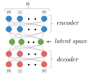
Figure 1: Encoding quantum probability distributions with VAEs. A VAE can be used to encode and then generate samples according to the probability distribution of a quantum state. Each dot corresponds to a neuron and neurons are arranged in layers. Input (top), latent, and output (bottom) layers contain $n$ neurons. The number of neurons in the other layers is a function of the compression and the depth. Layers are fully connected with each other with no intra layer connectivity. The network has three main components: the encoder (blue neurons), the latent space (green), and the decoder (red). Each edge of the network is labelled by a weight $\theta$. The total number of weights $m$ in the decoder corresponds to the number of parameters used to represent a quantum state. The network can approximate quantum states using $m<2^{n}$ parameters. The model is trained using a dataset consisting of basis elements drawn according to the probability distribution of a quantum state. Elements of the basis are presented to the input layer on top of the encoder and, during the training phase, the weights of the network are optimized in order to reconstruct the same basis element in the output layer.

Hard and easy quantum states

In this section we introduce a method to classify quantum states based on the hardness of sampling their probability distribution in a given basis. This will be used to assess the power of deep neural network models at representing many-body wave-functions.

We now proceed to define two concepts that will be frequently used throughout the paper and form the basis of our classification method: reconstruction accuracy and compression. Let $\rho$ and $\sigma$ be $n$–qubit quantum states. We say that $\sigma$ is a good representation of $\rho$ if the fidelity $F=\mathrm{Tr}(\sqrt{\rho^{1/2}\sigma\rho^{1/2}})\geq 1-\epsilon$ for an $\epsilon>0$. This accuracy metric cannot be immediately applied to the analysis of VAEs, that can only encode the probability distribution associated to a state. We now show that the fidelity can expressed in terms of the probability distributions over a measurement that maximally distinguishes the two states. Let $E=\{E_{i}\}$ be a POVM measurement. Then, using a result by Fuchs and Caves fuchs1994ensemble we can write

$$F=\min_{E}\sum_{i}\sqrt{\mathrm{Tr}(E_{i}\rho)\mathrm{Tr}(E_{i}\sigma)},$$ (2)

where the minimum is taken over all possible POVMs. Note that $p(i)=\mathrm{Tr}(E_{i}\rho)$ and $q(i)=\mathrm{Tr}(E_{i}\sigma)$ are the probabilities of measuring the state $\rho$ and $\sigma$, respectively, in outcome labelled by $i$ and $\sum_{i}\sqrt{p(i)q(i)}$ is the Bhattacharyya coefficient between the two distributions.

Using Eq. 2 we can relate the complexity of a state with the problem of estimating the fidelity $F$. This corresponds to the hardness of sampling the probability distribution $p(i)=\mathrm{Tr}(E^{\prime}_{i}\rho)$, where $E^{\prime}$ minimises Eq. 2 (here we assume that sampling from the approximating distribution $q(i)$ is at most as hard as sampling from $p(i)$).

Throughout the paper, unless where explicitly mentioned, we will work with states that have only positive, real entries in the computational basis. In this case, it is easy to see that the Bhattacharyya coefficient between the distributions reduces to the fidelity and, hence, measurements in the $Z$ basis minimises Eq 2.

We remark that, if it is not possible to find a POVM for which Eq. 2 is minimised it is always possible to use the standard formulation of the fidelity as a metric in the context of VAEs. This can be accomplished by making use of $3$ VAEs to encode the state $\sigma$ over $3$ different basis. By using standard tomographic techniques, like maximum likelihood, measurements in a complete basis can be used to reconstruct the full density matrix.

In order to connect the above definition of state complexity with VAEs we introduce the compression factor. Given an $n$-qubit state that is represented by a VAE with $m$ parameters in the decoder, the compression factor is $C=\frac{m}{2^{n}}$. We say that a state $\rho$ is exponentially compressible if there exists a network that approximates $\rho$ with high accuracy using $m=O(\mathrm{poly}(n))$ parameters.

Once a network is trained, the cost of generating a sample is proportional to the number of parameters in the network. In this sense the complexity of a state is parametrised by the number of parameters used by a neural network representation. Based on these observation we define easy states those that can be represented with high accuracy and exponential compression and hard states those that can be represented with high accuracy using at least $O(\mathrm{exp}(n))$ parameters. The last category includes: 1) states that can be efficiently sampled with a quantum computer, but are conjectured to have no classical algorithm to do so; 2) states that cannot be efficiently obtained on a quantum computer starting from some fixed product input state (e.g. random states).

Under this definition, states that admit an efficient classical description (such as stabilizer states or MPS with low bond dimension) are easy, because we known that $O(\mathrm{poly}(n))$ parameters are sufficient to specify the state. Specifically, for the class of easy states we consider separable states obtained by taking the tensor product of $n$ different $1$-qubit random states. More formally, we consider states of the form $\ket{\tau}=\bigotimes_{i=1}^{n}\ket{r_{i}}$ where $\ket{r_{i}}$ are random $1$-qubit states. These states can be described using only $2n$ parameters.

Among the class of hard states of the first kind, we study the learnability of a type of hard distributions introduced in fefferman2014power which can be sampled exactly on a quantum computer. These distributions are conjectured to be hard to approximately sample from classically – the existence of an efficient sampler would lead to the collapse of the Polynomial Hierarchy under some natural conjectures described in fefferman2014power ; aaronson2011computational . We discuss how to generate this type of states in the Methods section.

Finally, for the second class of hard states, we consider random pure states. These are generated by normalizing a $2^{n}$ dimensional complex vector drawn from the unit sphere according to the Haar measure.

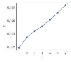
(a)

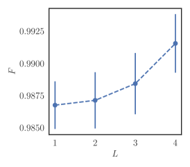
(b)

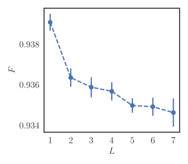
(c)

Figure 2: Depth affects the learnability of hard quantum states. Fidelity as a function of the number of layers in the VAE decoder for (a) an $18$-qubit hard state that is easy to generate with a quantum computer, (b) random $18$-qubit product states that admit efficient classical descriptions and (c) random $15$-qubit pure states. Errors bars for (b) and (c) show the standard deviation for an average of $5$ different random states. The compression level $C$ is set to $C=0.5$ for (a) and (c) and $C=0.015$ for (b) where $C$ is defined by $\frac{m}{2^{n}}$ where $m$ is the number of parameters in the VAE decoder and $n$ is the number of qubits. We use a lower compression rate for product states because, due to their simple structure, even a $1$ layer network achieves almost perfect overalp. Plot (b) makes use of up to 4 layers in order to avoid the saturation effects discussed in the Methods section.

Results

The role of depth in compressibility

Classically, depth is known to play a significant role in the representational capability of a neural network. Recent results, such as the ones by Mhaskar, Liao, and Poggio mhaskar2016learning , Telgarsky telgarsky2016benefits , and Eldan and Shamir eldan2016power showed that some classes of functions can be approximated by deep networks with the same accuracy as shallow networks but with exponentially less parameters.

The representational capability of networks that represent quantum states remains largely unexplored. Some of the known results are only based on empirical evidence and sometimes yield to unexpected results. For example, Morningstar and Melko morningstar2017deep showed that shallow networks are more efficient than deep ones when learning the energy distribution of a $2$-dimensional Ising model.

In the context of the learnability of quantum states Gao and Duan gao2017efficient proved that DBMs can efficiently represent some states that cannot be efficiently represent by shallow networks (i.e. states generated by polynomial depth circuits or $k$-local Hamiltonians with polynomial size gap) using a polynomial number of hidden units. However, there are no known methods to sample efficiently from DBMs when the weights include complex-valued coefficients.

We benchmark with numerical simulations the role played by depth in compressing states of different levels of complexities. We focus on three different states: an easy state (the completely separable state discussed in the previous section), a hard state (according to Fefferman and Umans), and a random pure state.

Our results are presented in Fig. 2. Here, by keeping the number of parameters in the decoder constant, we determine the reconstruction accuracy of networks with increasing depth. Remarkably, depth affects the reconstruction accuracy of hard quantum states. This might indicate that VAEs are able to capture correlations in hard quantum states. As a sanity check we notice that the network can learn correlations in random product states and that depth does not affect the learnability of random states.

Our simulations suggest a further link between neural network and quantum states. This topic has recently received the attention of the community. Specifically, Levine et al. levine2017deep demonstrated that convolutional rectifier networks with product pooling can be described as tensor networks. By making use graph theoretic tools they showed that nodes in different layers model correlations across different scales and that adding more nodes to deeper layers of a network can make it better at representing non-local correlations.

Efficient compression of physical states

In this section we focus our attention onto two questions: can VAEs find efficient representations of easy states? What level of compression can we obtain for hard states? Through numerical simulations we show that VAEs can learn to efficiently represent some easy states (that are challenging for standard methods) and achieve good levels of compressions for hard states. Remarkably, our methods allow to compress up to a factor $5$ the hard quantum states introduced in fefferman2015power . We remark that the exponential hardness cannot be overcome for general quantum states and our methods achieve only a factor improvement on the overall complexity. This may nevertheless be sufficient to be used as a characterisation tool where full classical simulation is not feasible.

We test the performance of the VAE representation on two classes of states: the hard states that can be constructed efficiently with a quantum computer introduced by Fefferman and Umans fefferman2015power and states that can be generated with a long-range Hamiltonian dynamics, as found for example in experiments with ultra-cold ions richerme2014non . The states generated through this evolution are highly symmetric physical states. However, due to the bond dimension increasing exponentially with the evolution time, these states are particularly challenging for MPS methods. An interesting question is to understand whether neural networks are able to exploit these symmetries and represent these states efficiently. We describe long-range Hamiltonian dynamics in the Methods section.

Results are displayed in Fig. 3. For states obtained through Hamiltonian evolution we achieve with almost maximum reconstruction accuracy compression levels of up to $C\approx 10^{-3}$. This corresponds to a number of parameters $m=\mathcal{O}(100)\ll 2^{18}$ which implies that the VAE has learned an efficient representation of the state.

In the case of hard state we can reach a compression of $0.2$, corresponding to a factor $5$ reduction in the number of parameters required to represent the state. Note that the entanglement properties of hard states are likely to make them hard to compress for tensor network states. For example, if one wanted to compress an $18$ qubits state using MPS (a type of tensor network that is known to be efficiently contractable) we have found that the estimated bond dimension to reconstruct this state is $D\approx 460$. This number is obtained computing the largest bipartite entanglement entropy ($S$), and estimating the bond dimension with $D\approx 2^{S}$. Considering that an MPS has $D^{2}$ variational parameters (in the best case), this would yield about $200$ thousands variational parameters required to represent those hard states. The resulting MPS compressing factor is then about $1.23$, a significantly lower figure with respect to the $5$ compression factor obtained with VAEs. We note that this calculation only shows that the entanglement structure of hard states is not well modelled by MPS. Other types of tensor networks might be more amenable to the specific structure of these states but it is unlikely these models will be computationally tractable.

Although limited, the levels of compression we achieve for hard states could play a role in experiments aimed at showing quantum supremacy. In this setting a quantum machine with a handful of noisy qubits performs a task that is not reproducible even by the fastest supercomputer. As recently highlighted by Montanaro and Harrow harrow2017quantum one of the key challenges with quantum supremacy experiments is to verify that the quantum machine is behaving as expected. Because quantum computers are conjectured to not be efficiently simulatable, verifying that a quantum machine is performing as expected is a hard problem for classical machines. The paper by Jozsa and Strelchuk jozsa2017efficient provides an introduction to several approaches to verification of quantum computation. Our methods might allow to characterise the result of a computation by reducing the complexity of the problem. Because any verification of quantum supremacy will likely involve a machine with only a few qubits above what can be efficiently classically simulated, even small reductions in the number of parameters of the state might allow to approximate relevant quantities in a computationally tractable way. Potentially, a neural network approach to verification can be accomplished by compressing a trusted initial state into a VAE whose parameters are then evolved according to a set of rules specified by the quantum circuit. By comparing the experimental distribution with the one sampled with the VAE it is then possible to determine whether the device is faulty. We remark that this type of verification protocol would only “approximately verify” the system because of the errors introduced during the compression phase.

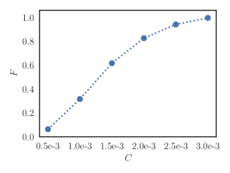
(a)

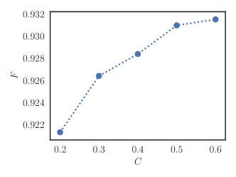
(b)

Figure 3: VAEs can learn efficient representation of easy states and can be used to characterize hard states. Fidelity as a function of compression $C=m/2^{n}$ for (a) an $18$-qubit state generated by evolving $2^{-n/2}\sum_{i}\ket{i}$ using the long-range Hamiltonian time evolution described in the Methods section for a time $t=20$ and (b) an $18$-qubit hard state generated according to fefferman2015power . Figure (a) shows that the VAE can learn to represent efficiently with almost perfect accuracy easy states that are challenging for MPS. Figure (b) shows that hard quantum states can be compressed with high reconstruction accuracy up to a factor $5$. The decoder in (a) has $1$ hidden layer to allow for greater compression without incurring in the saturation effects discussed in Methods section. The decoder in (b) has $6$ hidden layers in order to maximise the representational capability of the network.

Discussion

In this work we introduced VAEs, a type of deep, generative, neural network, as way to encode the probability distribution of quantum states. Our methods are completely unsupervised, i.e. do not require a labelled training set. By means of numerical simulations we showed that deep networks can represent hard quantum states that can be efficiently obtained by a quantum computer better than shallow ones. On the other hand, for states that are hard and conjectured to be not efficiently producible by quantum computers, depth does not appear to play a role in increasing the reconstruction accuracy. Our results suggest that neural networks are able to capture correlations in states that are provably hard to sample from for classical computers but not for quantum ones. As already pointed out in other works, this might signal that states that can be produced efficiently by a quantum computer have a structure that is well represented by a layered neural network.

Through numerical experiments we showed that our methods have two important features. First, they are capable of representing, using fewer parameters, states that that are known to have efficient representation but where other classical approaches struggle. Second, VAEs can compress hard quantum states up to a constant factor. However low, this compression level might enable to approximately verify quantum states of a size expected on near future quantum computers.

Presently, our methods allow to encode only the probability distribution of a quantum state. Future research should focus on developing VAE architectures that allow to reconstruct the full set of amplitudes. Other interesting directions involve finding methods to compute the quantum evolution of the parameters of the network and investigating whether the depth of a quantum circuit is related to the optimal depth of a VAE learning its output states. Finally, it is interesting to investigate how information is encoded in the latent layers of the network. Such analysis might provide novel tools to understand the information theoretic properties of a quantum system.

Methods

Numerical experiments

All our networks were trained using the tensorflow r1.3 framework on a single NVIDIA K80 GPU. Training was performed using backpropagation and the Adam optimiser with initial learning rate of $10^{-3}$ kingma2014adam . Leaky rectified linear units (LReLU) function were used on all hidden layers with the leak set to $0.2$ maas2013rectifier . Sigmoid activation functions were used on the final layer.

Training involves optimising two objectives: the reconstruction loss and the regularization loss. We used a warm up schedule on the regularisation objective by increasing a weight on the regularisation loss from $0$ to $0.85$ linearly during training  sonderby2016ladder . This turned out to be critical, especially for hard states. A consequence of this approach is that the model does not learn the distribution until close to the end of training irrespective of the number of training iterations. Each network was trained using $50,000$ batches of $1000$ samples each. Each sample consists of a binary string representing a measurement outcome.

Following training the state was reconstructed from the VAE decoder by drawing $100(2^{n})$ samples from a multivariate Gaussian with zero mean and unit variance. The samples were decoded by the decoder to generate measurement outcomes in the form of binary strings. The relative frequency of each string was recorded and used to reconstruct the learned distribution which was compared to the true distribution to determine its fidelity.

In all experiments the number of nodes in the latent layer is the same as the number of qubits. Using fewer or more nodes in this layer resulted in worse performance. The number of nodes in the hidden layers is determined by the number of layers and the compression $C$ defined by $\frac{m}{2^{n}}$ where $n$ is the number of qubits and $m$ is the number of parameters in the decoder. In all cases the encoder has the same number of hidden layers and nodes in each layer as the decoder.

We compress the VAE representation of a quantum state by removing neurons from each hidden layer of the VAE. For small $n$’s achieving a high level of compression caused instabilities in the network (i.e. the reconstruction accuracy became more dependent on the weight initialisation). In this respect we note that, by restricting the number of neurons in the penultimate layer, we are effectively constraining the number of possible basis states that can be expressed in the output layer and, as a result, the number of configurations the VAE can sample from. This can be shown noting that the activation functions of the penultimate layer generate a set of linear inequalities that must be simultaneously satisfied. A geometric argument that involves how many regions of an $n$-dimensional space $m$ hyperplanes can separate lead to conclude that, to have full expressive capability, the penultimate layer must include at least $n$ neurons. Similar arguments have been discussed in huang1991bounds for multilayer perceptrons.

States that are classically hard to sample from

We study the learnability of a special class of hard states introduced by Fefferman and Umans fefferman2015power which is produced by a certain quantum computational processes which exhibit quantum “supremacy”. The latter is a phenomenon whereby a quantum circuit which consists of quantum gates and measurements on a constant number of qubit lines samples from a particular class of distributions which is known to be hard to sample from on a classical computer modulo some very plausible computational complexity assumptions. To demonstrate quantum supremacy one only requires quantum gates to operate within a certain fidelity without full error-correction. This makes efficient sampling from such distributions feasible to execute on near-term quantum devices and opens the search for possibilities to look for practically-relevant decision problems.

To construct a distribution one starts from an encoding function $h:[m]\to\{0,1\}^{N}$. The function $h$ performs an efficient encoding of its argument and is used to construct the following so-called efficiently specifiable polynomial on $n$ variables:

$$Q(X_{1},\dots,X_{N})=\sum_{z\in[m]}X_{1}^{h(z)_{1}}\dots X_{N}^{h(z)_{N}},$$ (3)

where $h(z)_{i}$ means that we take only the $i$-th bit, and $m$ is an arbitrary integer. In the following, we pick $h$ to be related to the permanent. More specifically, $h:[0,n!-1]\to\{0,1\}^{n^{2}}$ maps the $i$-th permutation (out of $n!$) to a string which encodes its $n\times n$ permutation matrix in a natural way resulting in a $N$-coordinate vector, where $N=n^{2}$. To encode a number $A\in[0,n!-1]$ in terms of its permutation vector we first represent $A$ in factorial number system to get $A^{\prime}$ obtaining the $N$-coordinate vector which identifies a particular permutation $\sigma$.

With the above encoding, our efficiently specifiable polynomial $Q$ will have the form:

$$Q(X_{1},\dots,X_{N})=\sum_{z\in[n!-1]}X_{1}^{h(z)_{1}}\dots X_{N}^{h(z)_{N}}.$$ (4)

Fix some number $L$ and consider the following set of vectors $y=(y_{1},\ldots,y_{N})\in[0,L-1]^{N}$ (i.e. each $y_{j}$ ranges between $0$ and $L-1$). For each $y$ construct another vector $Z_{y}=(z_{y_{1}},\dots,z_{y_{N}})$ constructed as follows: each $z_{y_{j}}$ corresponds to a complex $L$-ary root of unity raised to power $y_{j}$. For instance, pick $L=4$ and consider $y^{\prime}=(1,2,3,0,2,3,0,4)$. Then the corresponding vector $Z_{y^{\prime}}=(w^{1},w^{2},w^{3},w^{0},w^{2},w^{3},w^{0},w^{4})$, where $w=e^{2\pi i/4}$ (for an arbitrary $L$ it will be $e^{2\pi i/L}$).

Having defined $Q$ fixed $L$ we are now ready to construct each element of the “hard” distribution ${\cal D}_{Q,L}$:

$$\text{Pr}_{{\cal D}_{Q,L}}[y]=\frac{|Q(Z_{y})|^{2}}{L^{N}n!}.$$ (5)

A quantum circuit which performs sampling is remarkably easy. It amounts to applying the quantum Fourier transform to a uniform superposition which was transformed by $h$ and measuring in the standard basis (see Theorem 4 of Section 4 of  fefferman2015power ).

Classical sampling of distributions based on the above efficiently specifiable polynomial is believed to be hard in particular because it contains the permanent problem. Thus, the existence of an efficient classical sampler would imply a collapse of the Polynomial Hierarchy to the third level (see Section 5 and 6 of fefferman2015power for detailed proof).

Long-range quantum Hamiltonians

The long-range Hamiltonian we consider has the form:

$$\left|\Psi(t)\right\rangle=e^{-i\mathcal{H}t}|\Psi(t=0)\rangle,$$ (6)

where

$$\mathcal{H}=\sum_{i<j}V(i,j)\left(\sigma_{i}^{x}\sigma_{j}^{x}+\sigma_{i}^{y}\sigma_{j}^{y}\right),$$ (7)

and $V(i,j)=1/|i-j|^{3/4}$ is a long-range two-body interaction, and the initial state is a fully polarized state is the product state $|\Psi(t=0)\rangle=2^{-n/2}\sum_{i}\ket{i}$. At long propagation times $t\gg 1$, the resulting states are highly entangled, and are for example, challenging for MPS-based tomography cramer2010efficient . To assess the ability of VAE to compress highly entangled states, we focus on the task of reconstructing the outcomes of experimental measurements in the computational basis. In particular, we generate samples distributed according to the probability density $|\Psi_{i}(t)|^{2}$, and reconstruct this distribution with our generative, deep models.

Acknowledgements.

We thank Carlo Ciliberto, Danial Dervovic, Alessandro Davide Ialongo, Joshua Lockhart, and Gillian Marshall for helpful comments and discussions. Andrea Rocchetto is supported by an EPSRC DTP Scholarship and by QinetiQ. Edward Grant is supported by EPSRC [EP/P510270/1]. Giuseppe Carleo is supported by the European Research Council through the ERC Advanced Grant SIMCOFE, and by the Swiss National Science Foundation through NCCR QSIT. Sergii Strelchuk is supported by a Leverhulme Trust Early Career Fellowship. Simone Severini is supported by The Royal Society, EPSRC and the National Natural Science Foundation of China.

Contributions.

The concept of using VAEs to encode probability distributions of quantum states was conceived by A.R., E.G., and G.C. The complexity framework was developed by A.R., G.C., and S.St. E.G. wrote the code and performed the simulations with help from S.St. The project was supervised by A.R. and S.Se. The first draft of the manuscript was prepared by A.R. and all authors contributed to the writing of the final version. A.R. and E.G. contributed equally to this work.

Competing Interests.

The authors declare no competing financial interests.

Data availability statements.

All data needed to evaluate the conclusions are available from the corresponding author upon reasonable request.

References

- (1) Nightingale, M. P. & Umrigar, C. J. Quantum Monte Carlo methods in physics and chemistry. 525 (Springer Science & Business Media, 1998).
- (2) Gubernatis, J., Kawashima, N. & Werner, P. Quantum Monte Carlo Methods (Cambridge University Press, 2016).
- (3) Suzuki, M. Quantum Monte Carlo methods in condensed matter physics (World scientific, 1993).
- (4) Verstraete, F., Murg, V. & Cirac, J. I. Matrix product states, projected entangled pair states, and variational renormalization group methods for quantum spin systems. Advances in Physics 57, 143–224 (2008).
- (5) Orús, R. A practical introduction to tensor networks: Matrix product states and projected entangled pair states. Annals of Physics 349, 117–158 (2014).
- (6) Carleo, G. & Troyer, M. Solving the quantum many-body problem with artificial neural networks. Science 355, 602–606 (2017).
- (7) Deng, D.-L., Li, X. & Das Sarma, S. Quantum Entanglement in Neural Network States. Physical Review X 7, 021021 (2017).
- (8) Nomura, Y., Darmawan, A., Yamaji, Y. & Imada, M. Restricted-Boltzmann-Machine Learning for Solving Strongly Correlated Quantum Systems. arXiv:1709.06475 (2017).
- (9) Deng, D.-L., Li, X. & Sarma, S. D. Exact Machine Learning Topological States. arXiv:1609.09060 (2016).
- (10) Glasser, I., Pancotti, N., August, M., Rodriguez, I. D. & Cirac, J. I. Neural Networks Quantum States, String-Bond States and chiral topological states. arXiv:1710.04045 (2017).
- (11) Kaubruegger, R., Pastori, L. & Budich, J. C. Chiral Topological Phases from Artificial Neural Networks. arXiv:1710.04713 (2017).
- (12) Torlai, G. et al. Many-body quantum state tomography with neural networks. arXiv preprint arXiv:1703.05334 (2017).
- (13) Perez-Garcia, D., Verstraete, F., Wolf, M. M. & Cirac, J. I. Matrix product state representations. arXiv preprint quant-ph/0608197 (2006).
- (14) Gao, X. & Duan, L.-M. Efficient representation of quantum many-body states with deep neural networks. Nature Communications 8, 662 (2017).
- (15) Chen, J., Cheng, S., Xie, H., Wang, L. & Xiang, T. On the Equivalence of Restricted Boltzmann Machines and Tensor Network States. arXiv:1701.04831 (2017).
- (16) Huang, Y. & Moore, J. E. Neural network representation of tensor network and chiral states. arXiv:1701.06246 (2017).
- (17) Clark, S. R. Unifying Neural-network Quantum States and Correlator Product States via Tensor Networks. arXiv:1710.03545 (2017).
- (18) Mhaskar, H., Liao, Q. & Poggio, T. Learning functions: When is deep better than shallow. arXiv preprint arXiv:1603.00988 (2016).
- (19) Telgarsky, M. Benefits of depth in neural networks. arXiv preprint arXiv:1602.04485 (2016).
- (20) Eldan, R. & Shamir, O. The power of depth for feedforward neural networks. In Conference on Learning Theory, 907–940 (2016).
- (21) Kingma, D. P. & Welling, M. Auto-encoding variational bayes. arXiv preprint arXiv:1312.6114 (2013).
- (22) Boixo, S. et al. Characterizing quantum supremacy in near-term devices. arXiv preprint arXiv:1608.00263 (2016).
- (23) Fuchs, C. A. & Caves, C. M. Ensemble-dependent bounds for accessible information in quantum mechanics. Physical Review Letters 73, 3047 (1994).
- (24) Fefferman, W. J. The power of quantum Fourier sampling. Ph.D. thesis, California Institute of Technology (2014).
- (25) Aaronson, S. & Arkhipov, A. The computational complexity of linear optics. In Proceedings of the forty-third annual ACM symposium on Theory of computing, 333–342 (ACM, 2011).
- (26) Morningstar, A. & Melko, R. G. Deep learning the ising model near criticality. arXiv preprint arXiv:1708.04622 (2017).
- (27) Levine, Y., Yakira, D., Cohen, N. & Shashua, A. Deep learning and quantum entanglement: Fundamental connections with implications to network design. arXiv preprint arXiv:1704.01552 (2017).
- (28) Fefferman, B. & Umans, C. The power of quantum fourier sampling. arXiv preprint arXiv:1507.05592 (2015).
- (29) Richerme, P. et al. Non-local propagation of correlations in quantum systems with long-range interactions. Nature 511, 198–201 (2014).
- (30) Harrow, A. W. & Montanaro, A. Quantum computational supremacy. Nature 549, 203–209 (2017).
- (31) Jozsa, R. & Strelchuk, S. Efficient classical verification of quantum computations. arXiv preprint arXiv:1705.02817 (2017).
- (32) Kingma, D. & Ba, J. Adam: A method for stochastic optimization. arXiv preprint arXiv:1412.6980 (2014).
- (33) Maas, A. L., Hannun, A. Y. & Ng, A. Y. Rectifier nonlinearities improve neural network acoustic models. In Proc. ICML, vol. 30 (2013).
- (34) Sønderby, C. K., Raiko, T., Maaløe, L., Sønderby, S. K. & Winther, O. Ladder variational autoencoders. In Advances in Neural Information Processing Systems, 3738–3746 (2016).
- (35) Huang, S.-C. & Huang, Y.-F. Bounds on the number of hidden neurons in multilayer perceptrons. IEEE transactions on neural networks 2, 47–55 (1991).
- (36) Cramer, M. et al. Efficient quantum state tomography. Nature communications 1, 149 (2010).