Linear hyperfine tuning of donor spins in silicon using hydrostatic strain

Abstract

We experimentally study the coupling of Group V donor spins in silicon to mechanical strain, and measure strain-induced frequency shifts which are linear in strain, in contrast to the quadratic dependence predicted by the valley repopulation model (VRM), and therefore orders of magnitude greater than that predicted by the VRM for small strains $|\varepsilon|<10^{-5}$. Through both tight-binding and first principles calculations we find that these shifts arise from a linear tuning of the donor hyperfine interaction term by the hydrostatic component of strain and achieve semi-quantitative agreement with the experimental values. Our results provide a framework for making quantitative predictions of donor spins in silicon nanostructures, such as those being used to develop silicon-based quantum processors and memories. The strong spin-strain coupling we measure (up to 150 GHz per strain, for Bi-donors in Si), offers a method for donor spin tuning — shifting Bi donor electron spins by over a linewidth with a hydrostatic strain of order $10^{-6}$ — as well as opportunities for coupling to mechanical resonators.

Donors in silicon present an attractive spin qubit platform, offering amongst the longest coherence times in the solid-state Tyryshkin et al. (2011); Saeedi et al. (2013) and single-qubit control with fault-tolerant fidelity Pla et al. (2013); Muhonen et al. (2015). As with the conventinal semiconductor industry, the majority of efforts in donor-based spin qubits are focused on ³¹P donors Kane (1998); O’Brien et al. (2001); Tyryshkin et al. (2003); Stegner et al. (2006); Morton et al. (2008); Simmons et al. (2011); Fuechsle et al. (2012); Büch et al. (2013). The heavier group V donors ⁷⁵As, ¹²¹Sb, and ²⁰⁹Bi have recently received substantial interest Franke et al. (2015, 2016); Wolfowicz et al. (2014); Singh et al. (2016); Morley et al. (2010); Mortemousque et al. (2014); Saeedi et al. (2015), offering larger nuclear spins (up to $I=9/2$ for ²⁰⁹Bi) and correspondingly richer Hilbert spaces that enable up to four logical qubits to be represented in a single dopant atom. Furthermore, “atomic clock transitions” have been identified in ²⁰⁹Bi where spin resonance transition frequencies become first-order insensitive to magnetic field noise, resulting in coherence times of up to 3 seconds in ²⁸Si Wolfowicz et al. (2013).

The exploitation of donor spins in silicon as qubits typically requires their incorporation into nano- and micro-electronic devices. This has been used to demonstrate single-shot readout of a single ³¹P donor spin using a tunnel-coupled silicon single-electron transistor (SET) Morello et al. (2010); Pla et al. (2012), and to create hybrid devices in which donor spins are coupled to superconducting resonators Bienfait et al. (2016); Eichler et al. (2017); Zollitsch et al. (2015) to develop interfaces between microwave photons and solid-state spins. In both cases, the use of metal-oxide-semiconductor (MOS) nanostructures Angus et al. (2007), or patterned superconducting films on silicon Bruno et al. (2015) involves a combination of materials with coefficients of thermal expansion that differ by up to an order of magnitude Lyon et al. (1977); Swenson (1983); Roberts (1982); NIS (1991); Nix and Macnair (1941). The presence of strain in the silicon environment around the donor spin is therefore pervasive when studying such nanodevices at cryogenic temperatures. Furthermore, factors such as optimising spin-resonator coupling or spin-readout speed motivate the placement of donors close to features such as SETs Morello et al. (2009) or resonator inductor wires Pla et al. (2016) where strain is maximal.

Strain modifies the band structure of silicon Bardeen and Shockley (1950); Herring and Vogt (1957), as has been shown, for example, to contribute to the confinement of single electrons in silicon under nanoscale aluminium gates Thorbeck and Zimmerman (2015); Veldhorst et al. (2015). The donor electron wavefunction is also modified by strain: following the valley repopulation model (VRM) developed by Wilson & Feher Wilson and Feher (1961b) within the framework of effective mass theory, an applied uniaxial strain lifts the degeneracy of the six silicon valleys leading to a mixture of the donor ground state, $1s(A_{1})$, with the first excited state, $1s(E)$. In this excited state, the hyperfine coupling between the donor electron and nuclear spin is zero, therefore the VRM predicts a quadratic reduction in $A$ as a function of uniaxial strain, as well as a strain-induced anisotropic contribution to the electron g-factor. Strain-induced perturbations of the donor hyperfine coupling have been observed for P-donor spins in ²⁸Si epilayers, grown on SiGe to yield built in strains of order 10^-3 Huebl et al. (2006) — piezoelectric contacts on such material have been used to modulate this built-in strain to shift the electron spin resonance frequency by up to $\sim 400$ kHz Dreher et al. (2011).

In this Letter, we report the observation of a strain-induced shift in the hyperfine coupling of group V donors in silicon which is linear (rather than quadratic), and therefore orders of magnitude greater than that predicted by the valley repopulation model of Wilson and Feher Wilson and Feher (1961b) for small strains ($|\varepsilon|\lesssim 10^{-5}$). We present experimental studies showing strain-tuning of the coherent evolution of each of the group V donor spins (³¹P, ⁷⁵As, ¹²¹Sb, and ²⁰⁹Bi), extracting the strain-induced shifts of the hyperfine coupling and electron spin g-factor for each, and corroborate the results with a combination of both tight binding and density functional theory calculations which reveal the crucial role of hydrostatic strain in this novel mechanism Pines et al. (1957). In addition to providing essential insights for the use of donor spins in nano- and micron-scale quantum devices, our results provide a method for linear tuning of the donor hyperfine interaction with coupling strengths of up to 150 GHz/strain for ²⁰⁹Bi donor spins.

The spin Hamiltonian for a group V donor in the presence of an external magnetic field $\mathbf{B}=B_{0}\mathbf{z}$ is:

$$\mathcal{\hat{H}}=\big{(}g_{e}\mu_{B}\mathbf{\hat{S}_{z}}-g_{n}\mu_{N}\mathbf{\hat{I}_{z}}\big{)}B_{0}+A\mathbf{\hat{S}}\cdot\mathbf{\hat{I}}$$ (1)

where $g_{e}$ and $g_{n}$ are, respectively, the electronic and nuclear g-factors, $\mu_{B}$ and $\mu_{N}$ are the Bohr and nuclear magnetons, $\mathbf{\hat{S}}$ and $\mathbf{\hat{I}}$ are the electronic and nuclear spin operators. The Fermi contact hyperfine interaction strength, $A=1.4754$ GHz in Si:Bi, can be expressed as:

$$A=\cfrac{8\pi}{3}g_{0}\mu_{B}g_{n}\mu_{N}|\psi(0)|^{2}$$ (2)

where $\psi(0)$ represents the amplitude of the electronic wavefunction at the nucleus and $g_{0}=2.0023$ is the free electron g-factor.The eigenstates of this Hamiltonian describe a Hilbert space of dimension $(2S+1)(2I+1)$, with $S=1/2$ and $I$ determined by the nuclear spin species, illustrated for the case of ²⁰⁹Bi:Si in Fig. 1(A). Transitions between these eigenstates obeying the selection rule ($\Delta m_{S},\Delta m_{I})=(\pm 1,0)$ in the high field limit can be driven and detected using pulsed electron spin resonance (ESR) Schweiger and Jeschke (2005).

Figure 1: (A) Energy levels of Si:Bi spin eigenstates as a function of magnetic field, with the ten allowed ESR transitions at 9.7 GHz highlighted and labelled according to their high-field nuclear spin projection $m_{I}$. (B) Schematic of experimental setup. The silicon single crystal sample is mounted between two engineered plastic rods with the ability to apply compressive stress. $\theta$, the angle of the applied magnetic field to the $[001]$ direction, can be varied by rotating the sample. (C) Observed linear frequency shifts for each of the ten allowed ESR transitions shown in panel (A), as a function of strain $\varepsilon_{11}$, with $\theta=30\degree$.

Figure 2: Electron spin echo signals in the frequency domain measured in ²⁸Si:Bi as a function of compressive strain (shown in terms of the uniaxial strain $\varepsilon_{11}$ and hydrostatic strain $\varepsilon_{\rm hs}$) arising from the applied stress in our experiment. Time-domain echoes for zero strain and $\varepsilon_{11}=1.4\times 10^{-5}$ are shown as insets. Data shown is from the $m_{I}=-1/2$ transition with $\theta=45\degree$, taken at $T=8$ K.

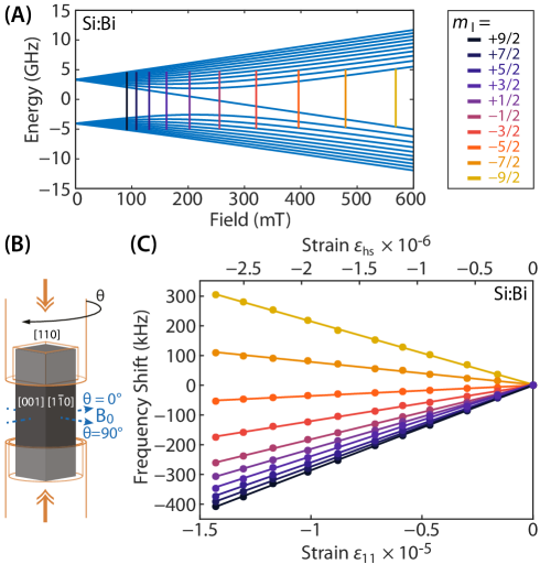
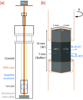
We use samples of isotopically enriched ²⁸Si doped with Bi, Sb, As and P (see Ref sup for more details), mounted with crystal orientation shown in Fig. 1(B). The sample is situated inside a dielectric microwave ESR resonator in an Oxford Instruments CF935 liquid helium flow cryostat, and is held between two PEEK rods whose end faces have been CNC-milled to match the profile of the sample allowing it to be rotated with respect to the magnetic field. Using calibrated masses, a uniaxial stress is applied to the sample perpendicular to the [110] face, via the upper rod which extends outside the cryostat. The resulting strain tensor can be derived from the generalised form of Hooke’s law for anisotropic materials and the compliance matrix for silicon Zhang et al. (2014): in the ([110],[1$\bar{1}$0],[001]) coordinate system per kg of applied mass, $\varepsilon_{11}=$-1.45\text{\times}{10}^{-5}$$/kg, $\varepsilon_{22}=$9.02\text{\times}{10}^{-7}$$/kg, $\varepsilon_{33}=$5.24\text{\times}{10}^{-6}$$/kg, and $\varepsilon_{i\neq j}=0$. While the VRM predicts frequency shifts only from uniaxial strain, we shall see that the new mechanism presented here arises from hydrostatic strain $\varepsilon_{\rm hs}=(\varepsilon_{11}+\varepsilon_{22}+\varepsilon_{33})/3$. In our setup, we estimate a strain per unit mass $\varepsilon_{\rm hs}=$-2.78\text{\times}{10}^{-6}$$/kg.

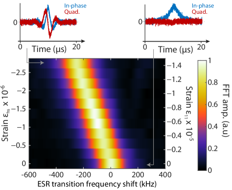
We use a home-built pulsed ESR spectrometer Ross (2017) at 9.7 GHz to apply a Hahn echo sequence $\pi/2\rightarrow\tau\rightarrow\pi\rightarrow\tau\rightarrow echo$ Hahn (1950), with $\tau=15~{}\mu$s and a $\pi$ pulse duration of 130 ns. The time-domain Hahn echo signals (top of Fig. 2) obtained while systematically increasing the applied strain are then Fourier transformed to yield the strain-induced shifts in spin resonance frequency sup .

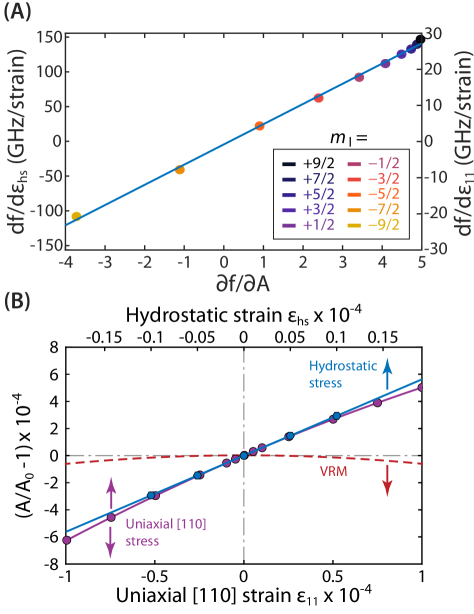
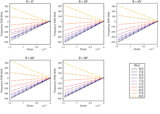
First, we observe in Fig. 2 that the Bi donor ESR transition can be shifted by more than a linewidth (in ²⁸Si) for strains of order 10^-5 (uniaxial) or 10^-6 (hydrostatic). We fit the frequency-domain echo signals to a Voigt profile, and then plot the centre-frequency shifts as a function of strain, for each of the ten allowed ESR transitions (see Fig. 1(C)). Strikingly, the ESR frequency of each transition shows a linear dependence on strain, rather than the expected quadratic dependence. In Fig. 3, we plot the experimentally determined $\partial f/\partial\epsilon_{11}$ for each transition against the first-order sensitivity of each transition frequency to the isotropic hyperfine coupling $\partial f/\partial A$. Remarkably, all 10 points fall on a single line, demonstrating that the dominant effect we observe in Si:Bi is a strain-induced shift in the isotropic hyperfine coupling which is linear in strain, and equivalent to $\partial A/\partial\varepsilon_{11}$ = $5.4\pm 0.3$ GHz or $\partial A/\partial\varepsilon_{\rm hs}$ = $28.2\pm 1.6$ GHz.

Figure 3: (A) The gradient of the strain-induced frequency shifts (d$f/$d$\epsilon$) for each of the ten Si:Bi ESR transitions are shown as a function of the first-order sensitivity of each transition to the hyperfine coupling ($\partial f/\partial A$). The linear relationship confirms the observed strain-induced shifts in Si:Bi result from tuning the hyperfine coupling, $A$, with a gradient $\partial A/\partial\epsilon_{11}=5.4\pm 0.3$ GHz or, equivalently, $\partial A/\partial\epsilon_{\rm hs}=28.2\pm 1.6$ GHz. (B) Calculations showing the relative change in hyperfine coupling strength $A/A_{0}$ as a function of strain, comparing tight-binding (TB) and valley repopulation (VRM) models. To mimic the experiment, we show TB calculations of $A/A_{0}$ under uniaxial stress along $[110]$ (purple curve and circles), which produces a hydrostatic component of strain ($\varepsilon_{\rm hs}$, top axis) in addition to a uniaxial component along $[110]$ ($\varepsilon_{\rm 11}$, bottom axis). This behaviour can be understood by comparing with TB calculations for pure hydrostatic stress (blue curve and hexagons), plotted on the same axis of $\varepsilon_{\rm hs}$, as well as calculations from the VRM (red dotted curve), plotted on the same axis of $\varepsilon_{\rm 11}$. The arrows indicate the relevant axes for each trace.

Multivalley effective mass theory (EMT) has been successful in describing many aspects of the donor electron wavefunction Kohn and Luttinger (1955); Luttinger and Kohn (1955); Pantelides and Sah (1974), including close agreement between theory and experimental measurements of the Stark effect Pica et al. (2014a) and predictions of exchange coupling between neighbouring donors Pica et al. (2014b). Within this framework, the wavefunction is expanded in terms of Bloch functions concentrated around the six degenerate [100] conduction band minima (valleys) such that $\psi=\sum_{\mu=1}^{6}\alpha_{\mu}F_{\mu}\phi_{\mu}$ where $\mu$ indexes over the valleys in the basis $[+x,-x,+y,-y,+z,-z]$, $F_{\mu}$ is a hydrogen-like envelope function, and $\phi_{\mu}$ is the valley Bloch function. The donor impurity potential breaks the symmetry of the crystal and induces a coupling between the valleys, leading to a valley-orbit splitting of the $1s$-like donor state into three sub-levels. The ground state is singly degenerate with $A_{1}$ symmetry and has $\alpha_{\mu}=1/\sqrt{6}$, while one of the excited states is doubly degenerate with $E$ symmetry and has $\alpha_{E_{1}}=1/2[1,1,-1,-1,0,0]$ and $\alpha_{E_{2}}=1/2[1,1,0,0,-1,-1]$. The valley repopulation model assumes that uniaxial strain applied along a valley axis results in the corresponding pair of valley energies being decreased or increased for compressive or tensile strain, respectively Wilson and Feher (1961b). This modification of the valley energies results in a redistribution of the amplitude of each valley contributing to the ground state, which can be represented under strain as an admixture of the $1s(A_{1})$ and $1s(E)$, resulting in a quadratic reduction of $A$ as a function of uniaxial strain. At our maximum applied strain of $\varepsilon_{11}=-1.45\times 10^{-5}$, the VRM predicts a reduction in $A$ of 1.9 kHz, while we measure a reduction in $A$ of 78 kHz — this discrepancy is even more pronounced for smaller strains. Therefore, in addition to predicting a different functional form of the dependence of $A$ against strain, the VRM predicts shifts which are approximately two orders of magnitude smaller than what we measure in this strain regime, implying that another physical mechanism must dominate the changes to the structure of the donor electron wavefunction we observe.

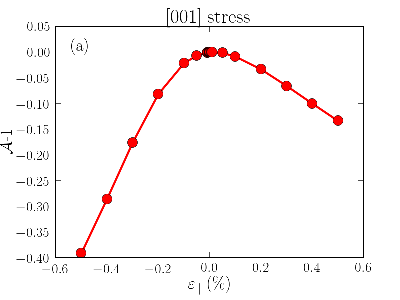
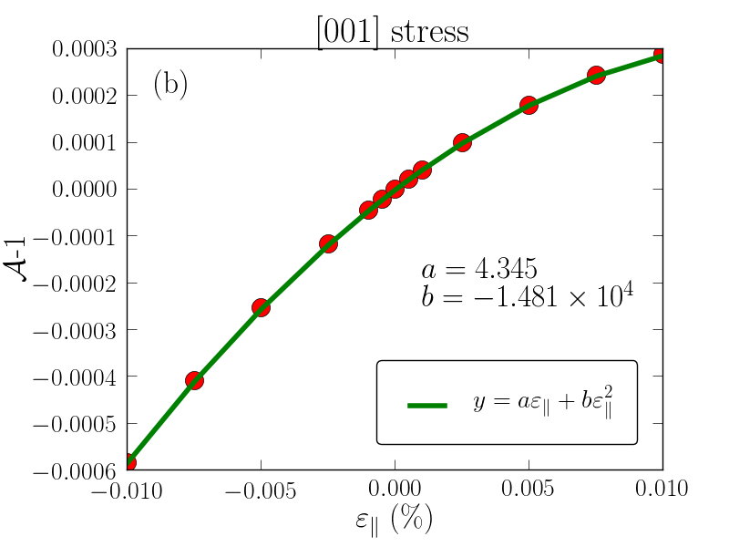
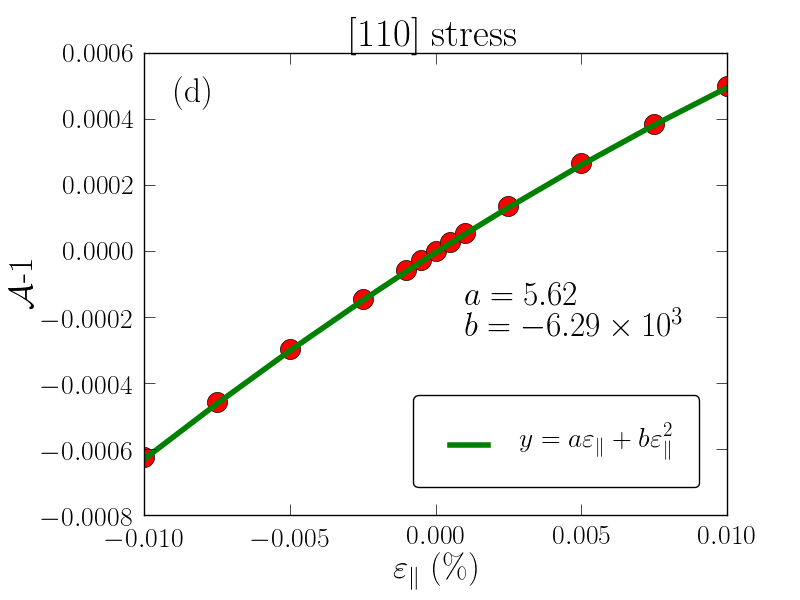
In order to understand these trends, we have computed the bound states of bismuth impurities in silicon using the $sp^{3}d^{5}s^{*}$ tight-binding (TB) model of Ref. Niquet et al., 2009. This model reproduces the variations of the band structure of bulk silicon under arbitrary strains in the whole first Brillouin zone. The impurity is described by a Coulomb tail and by a correction of the orbital energies of the bismuth atom (similar to a central cell correction in the effective mass approximation) Usman et al. (2015). The TB ratio $A/A_{0}$ between the strained ($A$) and unstrained ($A_{0}$) hyperfine interaction strengths is plotted in Fig. 3(B) under uniaxial stress along $[110]$, as a function of the resulting uniaxial $[110]$ and hydrostatic strains. Surprisingly, and in agreement with the experiments performed here, $A/A_{0}$ behaves linearly with small strain, and this trend can be assigned to the effects of the hydrostatic stress. Although not predicted by the VRM, the existence of a linear hydrostatic term is compatible with the symmetries of the system Pines et al. (1957). A symmetry analysis indeed suggests that, to second order in the strains $\varepsilon_{ij}$ in the cubic axis set:

$$A/A_{0} =1+\frac{K}{3}(\varepsilon_{xx}+\varepsilon_{yy}+\varepsilon_{zz})$$

$$+\frac{L}{2}\left[(\varepsilon_{yy}-\varepsilon_{zz})^{2}+(\varepsilon_{xx}-\varepsilon_{zz})^{2}+(\varepsilon_{xx}-\varepsilon_{yy})^{2}\right]$$

$$+N(\varepsilon_{yz}^{2}+\varepsilon_{xz}^{2}+\varepsilon_{xy}^{2})\,.$$ (3)

A fit to the TB data yields $K=29.3$, $L=-9064$ and $N=-225$. $L$ mostly results from the coupling of the $1s(A_{1})$ with the $1s(E)$ state by the uniaxial strain. The TB $L$ is close to the VRM $L=-2\Xi_{u}^{2}/(9\Delta^{2})=-9720$ Wilson and Feher (1961b), where $\Xi_{u}=8.6$ eV is the uniaxial deformation potential of the conduction band of silicon and $\Delta=41$ meV is the splitting between the $1s(A_{1})$ and the $1s(E)$ state of the Bi impurity. The quadratic shear term $N$ is usually negligible with respect to $L$. $K=\partial(A/A_{0})/\partial\varepsilon_{\rm hs}$ results from the coupling of the $1s(A_{1})$ with the $2s(A_{1})$ state (and higher $A_{1}$ states, since hydrostatic strain preserves the symmetry of the system) due to the change of the shape and depth of the central cell correction under strain. $A/A_{0}$ is dominated by this hydrostatic term at small strain, as evidenced in Fig. 3(B). The TB $K=29.3$ is larger than the experimental $K=19.1$. At variance with $L$ (which mostly depends on a deformation potential of the silicon matrix), $K$ indeed depends on details of the potential near the impurity, which must be specifically accounted for in the TB model in order to reach quantitative accuracy sup . In order to better capture the central cell correction around the bismuth impurity, we also performed first principles calculations using density functional theory (DFT) to describe the atomic relaxations not accounted for by our TB calculations sup . The DFT calculations further corroborate the linear dependence of the hyperfine coupling on hydrostatic strain (for $\epsilon_{\rm hs}\leq 10^{-3}$), and predict a coefficient $K=17.5$, in good agreement with our experiments. Full details concerning the models and calculations can be found in Ref sup .

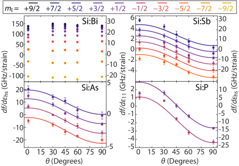
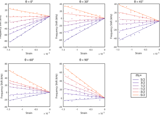
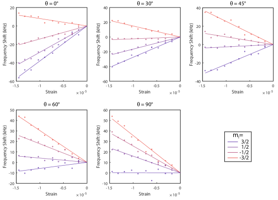
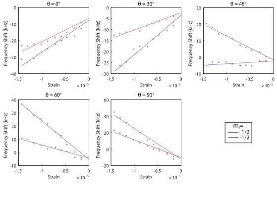
To test our model further and explore the expected anisotropy of a g-factor coupling to strain, we extend our study over a range of magnetic field orientations (as defined in Fig. 1(B)) and for the other group V donors: ³¹P, ⁷⁵As, and ¹²¹Sb. In all cases we find the observed ESR transition frequency shifts $f$ are linear as a function of hydrostatic strain $\epsilon_{\rm hs}$, with the resulting coupling strengths ($df/d\epsilon_{\rm hs}$) summarised in Fig. 4 and Table SI, along with values predicted from tight-binding calculations and full data sets sup . While we find no significant anisotropy in Si:Bi, the data from Si:Sb, Si:As, and Si:P display strain effects which clearly depend on the magnetic field orientation, attributed to a strain-induced anisotropic electronic g-factor. Following Wilson & Feher Wilson and Feher (1961b), our model for this anisotropy includes a term accounting for the effect of valley repopulation, and another accounting for the effect of spin-orbit coupling in the sheared lattice. Fits of this model to our experimental data reproduce the predicted strength of both of these effects to within a factor of two sup .

Figure 4: Extracted linear fit gradients d$f/$d$\epsilon_{11}$ for each transition for all four donors under consideration as a function of the angle of $B_{0}$ w.r.t. the crystal $\theta$. For Si:Sb, Si:As, and Si:P, these fits are overlaid with a model taking into account the linear shift of hyperfine interaction strength $A$ as well as an anisotropic g-factor as a function of $\epsilon_{11}$.

Through experiments and calculations, we have demonstrated that hydrostatic strain in silicon leads to a strong, linear tuning of the hyperfine interaction in group V donors, through coupling between the $1s(A_{1})$ and $2s(A_{1})$ states. The ability to shift the ESR transition frequencies by over a linewidth with hydrostatic strain in the order of $10^{-6}$ opens up new possibilities for conditional “A-gate” control of donors as well as coupling to mechanical resonators. In addition, these insights will be crucial in supporting the design of quantum memories and processors based on donors in silicon, enabling the ability to accurately predict ESR transition energies as a function of donor position within the device structure.

We acknowledge helpful discussions with Ania Jayich. This research was supported by the Engineering and Physical Sciences Research Council (EPSRC) through UNDEDD (EP/K025945/1) and a Doctoral Training Grant; as well as by the European Union’s Horizon 2020 research and innovation programme under Grant Agreement No 688539 (http://mos-quito.eu) and the European Community’s Seventh Framework Programme Nos. 279781 (ASCENT) and 615767 (CIRQUSS); and also by the Agence Nationale de la Recherche through project QIPSE.

Supplementary Materials: Linear hyperfine tuning of donor spins in silicon using hydrostatic strain

I Experimental methods

The sample ‘Bi’ is a $2\times 2\times 10$ mm single crystal of isotopically purified ²⁸Si doped with $4.4\text{\times}{10}^{14}$ Bi donors/cm³, and ‘Buffet’ is a $2\times 2\times 7$ mm ²⁸Si single crystal doped with $1.5\text{\times}{10}^{14}$ ³¹P donors/cm³, $5\text{\times}{10}^{14}$ ⁷⁵As donors/cm³, and $1.1\text{\times}{10}^{14}$ ¹²¹Sb donors/cm³.

A cylindrical aluminium plate rests on the floor of the cryostat (see Fig. S1). A rod made from the plastic PEEK screws into this plate and extends into the centre of the sapphire resonator, providing a bottom support for the sample. A second PEEK rod, which is supported radially by the resonator structure but is free to move along its axial direction, holds the sample in place from above.

Each echo is averaged 300 times and the spins are reset after each cycle with a 5 ms flash of 50 mW above-bandgap 1047 nm laser light through an optical window in the cryostat.

The time-domain Hahn echo signals can be expressed as a periodic oscillation at the frequency of the detuning between the fixed microwave drive frequency and the strain-shifted transition frequency, multiplied by an envelope function given by the inverse Fourier transform of the frequency-domain transition spectral lineshape. Then, by the convolution theorem, the Fourier transform of such a signal results in a frequency-domain spectral peak centred at the detuning frequency. The strain-induced detuning is then extracted by fitting a Voigt profile to this spectral peak. See Ref. Schweiger and Jeschke (2005) Chapter 5 for more details.

Figure S1: a) Schematic of experimental setup showing Bruker ESR resonator mounted inside liquid Helium flow cryostat. The sample is held in place in the centre of the sapphire resonator by two engineered plastic rods. b) Magnified view of sample inside strain mount.

II Tight-binding modeling

II.1 Model

We consider a single bismuth impurity at the center of a large box of silicon with side $L=48a\simeq 26$ nm ($a=5.431$Å being the lattice parameter of silicon).

The electronic structure of silicon is described by the $sp^{3}d^{5}s^{*}$ tight-binding (TB) model of Ref. Niquet et al., 2009. This model reproduces the effects of arbitrary strains on the band edges and effectives masses of silicon. Note that this model includes two $s$ orbitals per atom (“$s$” and “$s^{*}$”).

The bismuth impurity is described by a Coulomb tail and an “on-site” chemical and Coulomb correction Roche et al. (2012); Usman et al. (2015). The expression of the Coulomb tail is based on the dielectric function proposed by Nara Nara and Morita (1966). The potential on atom $i$ reads:

$$V_{i}=V(R_{i})\text{\ with\ }V(r)=-\frac{e^{2}}{\kappa r}\left(1+A\kappa e^{-\alpha r}+(1-A)\kappa e^{-\beta r}-e^{-\gamma r}\right)\,,$$ (S1)

where $\vec{R}_{i}$ is the position of the atom (the bismuth impurity being at $\vec{R}_{1}=\vec{0}$), $\kappa=11.7$ is the dielectric constant of silicon, $A=1.175$, $\alpha=0.757$ Bohrs^-1, $\beta=0.312$ Bohrs^-1, and $\gamma=2.044$ Bohrs^-1 Nara and Morita (1966); Bernholc and Pantelides (1977). This expression deviates from a simple $-e^{2}/(\kappa R_{i})$ tail mostly on the first and second nearest neighbors of the bismuth atom.

The “on-site” correction is a shift of the energies of the bismuth orbitals that accounts for the different chemical nature of the impurity and for the short-range part of the Coulomb tail. This shift $\Delta E=-U$ reads for each orbital:

$$U_{s}=5.862\ \rm{eV}$$

$$U_{p}=3.690\ \rm{eV}$$

$$U_{d}=0.000\ \rm{eV}$$

$$U_{s^{*}}=5.862\ \rm{eV}\,.$$ (S2)

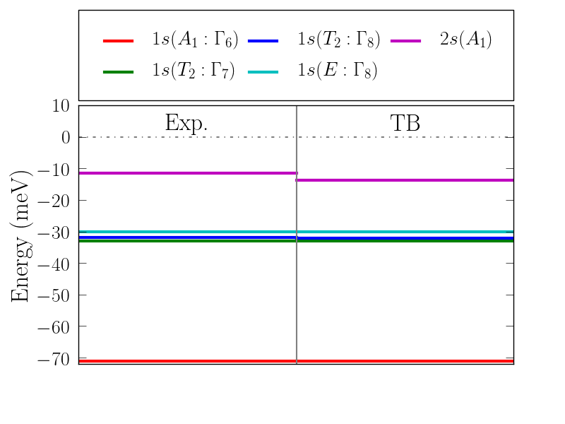
These values were adjusted on the experimental binding energies of the $1s(A_{1})$, $1s(E)$ and $1s(T_{2})$ states of bismuth in silicon (see Fig. S2) Krag et al. (1970); Ramdas and Rodriguez (1981); Zhukavin et al. (2011). We have set $U_{s}=U_{s^{*}}$ on purpose since it is practically difficult to adjust $U_{s}$ and $U_{s^{*}}$ separately. We have designed an other model with $U_{s^{*}}=0$ that gives very similar results.

We include spin-orbit coupling (SOC) in the calculations. SOC is described by an intra-atomic Hamiltonian acting on the $p$ orbitals of each atom, $H_{\rm SO}=\lambda\vec{L}_{i}\cdot\vec{S}$, where $\vec{S}$ is the spin, $\vec{L}_{i}$ the angular momentum on atom $i$, $\lambda=0.0185$ eV for silicon, and $\lambda=0.350$ eV for bismuth (adjusted on the experimental spin splittings of bismuth in silicon Zhukavin et al. (2011)).

Figure S2: Experimental (Exp.) and TB bound states of a bismuth impurity in silicon. The horizontal dash-dotted line is the bulk conduction band edge.

The hyperfine coupling constant $A$ is proportional to the probability of presence $|\Psi(\vec{0})|^{2}$ of the electron on the bismuth nucleus [Eq. (2) of main text]. In the TB framework,

$$\left|\Psi(\vec{0})\right|^{2}=\left|c_{s}s(\vec{0})+c_{s^{*}}s^{*}(\vec{0})\right|^{2}=\left|c_{s}\right|^{2}\left|s(\vec{0})\right|^{2}\left|1+\frac{c_{s^{*}}}{c_{s}}\frac{s^{*}(\vec{0})}{s(\vec{0})}\right|^{2}\,,$$ (S3)

where $c_{s}$ and $c_{s^{*}}$ are the coefficients of the $s$ and $s^{*}$ orbitals of the bismuth atom in the TB wavefunctions (we discard the spin index here for the sake of simplicity). This expression is, in principle, ambiguous because the radial parts of the $s$ and $s^{*}$ orbitals of the TB model are not explicitly known. We have tentatively set $R_{s^{*}s}=s^{*}(\vec{0})/s(\vec{0})=0.058$ Usman et al. (2015). Yet the choice for $R_{s^{*}s}$ is practically little relevant, as $c_{s^{*}}/c_{s}$ is almost independent on the strains $\hat{\varepsilon}=\{\varepsilon_{xx},\varepsilon_{yy},\varepsilon_{zz},\varepsilon_{yz},\varepsilon_{xz},\varepsilon_{xy}\}$. Therefore, the quantity

$${\cal A}(\hat{\varepsilon})=\frac{A(\hat{\varepsilon})}{A_{0}}=\frac{\left|\Psi(\vec{0},\hat{\varepsilon})\right|^{2}}{\left|\Psi(\vec{0},\hat{\varepsilon}=0)\right|^{2}}\,,$$ (S4)

which describes the relative change of the hyperfine coupling constant under strains, is well defined within TB, irrespective of the assumptions made for the radial parts of the $s$ and $s^{*}$ orbitals.

II.2 Strains

We consider uniaxial stress along $[001]$ and $[110]$.

For uniaxial stress $\sigma_{zz}=\sigma_{\parallel}$ along $[001]$, the infinitesimal strains in the cubic axis set can be found from Hooke’s law $\sigma_{xx}=\sigma_{yy}=0$:

$$\varepsilon_{zz} =\varepsilon_{\parallel}=\frac{c_{11}+c_{12}}{(c_{11}-c_{12})(c_{11}+2c_{12})}\sigma_{\parallel}$$ (S5a)

$$\varepsilon_{xx}=\varepsilon_{yy} =\varepsilon_{\perp}=-\frac{c_{12}}{c_{11}+c_{12}}\varepsilon_{\parallel}\,,$$ (S5b)

where $c_{11}=166$ GPa, $c_{12}=64$ GPa and $c_{44}=79.6$ GPa are the elastic constants of bulk silicon.

For uniaxial stress along $[110]$, the infinitesimal strains in the $\{1\equiv[110],\,2\equiv[1\bar{1}0],\,3\equiv[001]\}$ axis set read:

$$\varepsilon_{11}=\varepsilon_{\parallel} =\frac{(c_{11}-c_{12})(c_{11}+2c_{12})+2c_{11}c_{44}}{4(c_{11}-c_{12})(c_{11}+2c_{12})c_{44}}\sigma_{\parallel}$$ (S6a)

$$\varepsilon_{22} =-\frac{(c_{11}-c_{12})(c_{11}+2c_{12})-2c_{11}c_{44}}{(c_{11}-c_{12})(c_{11}+2c_{12})+2c_{11}c_{44}}\varepsilon_{\parallel}$$ (S6b)

$$\varepsilon_{33} =-\frac{4c_{12}c_{44}}{(c_{11}-c_{12})(c_{11}+2c_{12})+2c_{11}c_{44}}\varepsilon_{\parallel}\,.$$ (S6c)

In the original cubic axis set, the strains are therefore:

$$\varepsilon_{xx}=\varepsilon_{yy} =\frac{2c_{11}c_{44}}{(c_{11}-c_{12})(c_{11}+2c_{12})+2c_{11}c_{44}}\varepsilon_{\parallel}$$ (S7a)

$$\varepsilon_{zz} =-\frac{4c_{12}c_{44}}{(c_{11}-c_{12})(c_{11}+2c_{12})+2c_{11}c_{44}}\varepsilon_{\parallel}$$ (S7b)

$$\varepsilon_{xy} =\frac{(c_{11}-c_{12})(c_{11}+2c_{12})}{(c_{11}-c_{12})(c_{11}+2c_{12})+2c_{11}c_{44}}\varepsilon_{\parallel}\,.$$ (S7c)

Note that there is an additional shear component with respect to uniaxial $[001]$ stress.

II.3 Results

Figure S3: (a, b) ${\cal A}(\varepsilon_{\parallel})$ for uniaxial $[001]$ stress on (a) large and (b) small scales. (c, d) ${\cal A}(\varepsilon_{\parallel})$ for uniaxial $[110]$ stress on (c) large and (d) small scales.

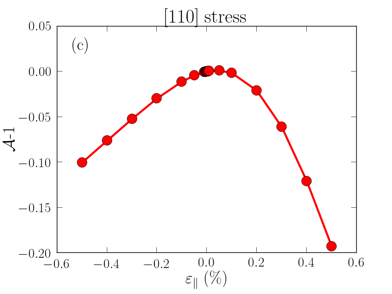
${\cal A}(\varepsilon_{\parallel})$ is plotted in Fig. S3 for uniaxial $[001]$ and $[110]$ stress.

In the valley repopulation model (VRM) Wilson and Feher (1961a), ${\cal A}(\varepsilon_{\parallel})$ is expected to be quadratic with small $\varepsilon_{\parallel}$ (the changes in ${\cal A}$ being exclusively driven by the loss of symmetries). In the TB approximation, ${\cal A}(\varepsilon_{\parallel})$ indeed describes a parabola for weak stress, but centered on some $\varepsilon_{\parallel}>0$. Therefore, ${\cal A}(\varepsilon_{\parallel})$ appears to behave almost linearly with small compressive $\varepsilon_{\parallel}$.

To understand this trend, it is very instructive to split the strain into a hydrostatic component, an uniaxial component, and a shear component. The hydrostatic component $\hat{\varepsilon}_{\rm hs}$ is defined as $\varepsilon_{xx}=\varepsilon_{yy}=\varepsilon_{zz}=\varepsilon_{\rm hs}$. It accounts for the changes in the total volume $\Omega$ ($\Delta\Omega/\Omega=3\varepsilon_{\rm hs}$). The uniaxial and shear components account for the changes in symmetries (at constant volume). The uniaxial component $\hat{\varepsilon}_{\rm uni}$ is defined as $\varepsilon_{zz}=\varepsilon_{\rm uni}$, $\varepsilon_{xx}=\varepsilon_{yy}=-\varepsilon_{\rm uni}/2$, and the shear component $\hat{\varepsilon}_{\rm shear}$ as $\varepsilon_{xy}=\varepsilon_{\rm shear}$.

For uniaxial stress along $[001]$ [Eqs. (S5)],

$$\varepsilon_{\rm hs}^{001} =\frac{k}{3}\varepsilon_{\parallel}$$ (S8a)

$$\varepsilon_{\rm uni}^{001} =\left(1-\frac{k}{3}\right)\varepsilon_{\parallel}\,,$$ (S8b)

where:

$$k=\frac{c_{11}-c_{12}}{c_{11}+c_{12}}\,.$$ (S9)

For uniaxial stress along $[110]$ [Eqs. (S6)],

$$\varepsilon_{\rm hs}^{110} =\frac{2k_{1}-k_{2}}{3}\varepsilon_{\parallel}$$ (S10a)

$$\varepsilon_{\rm uni}^{110} =-\frac{2(k_{1}+k_{2})}{3}\varepsilon_{\parallel}$$ (S10b)

$$\varepsilon_{\rm shear}^{110} =(1-k_{1})\varepsilon_{\parallel}$$ (S10c)

where:

$$k_{1} =\frac{2c_{11}c_{44}}{(c_{11}-c_{12})(c_{11}+2c_{12})+2c_{11}c_{44}}$$ (S11a)

$$k_{2} =\frac{4c_{12}c_{44}}{(c_{11}-c_{12})(c_{11}+2c_{12})+2c_{11}c_{44}}\,.$$ (S11b)

Figure S4: ${\cal A}(\hat{\varepsilon})$ for (a) hydrostatic strain ($\varepsilon=\varepsilon_{\rm hs}$), (b) uniaxial ($\varepsilon=\varepsilon_{\rm uni}$) and shear strain ($\varepsilon=\varepsilon_{\rm shear}$).

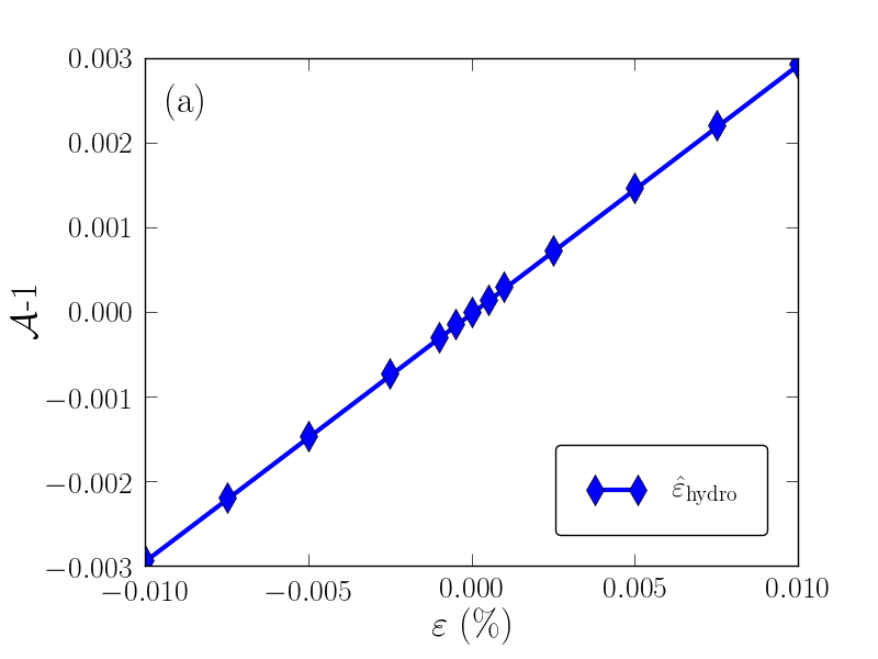
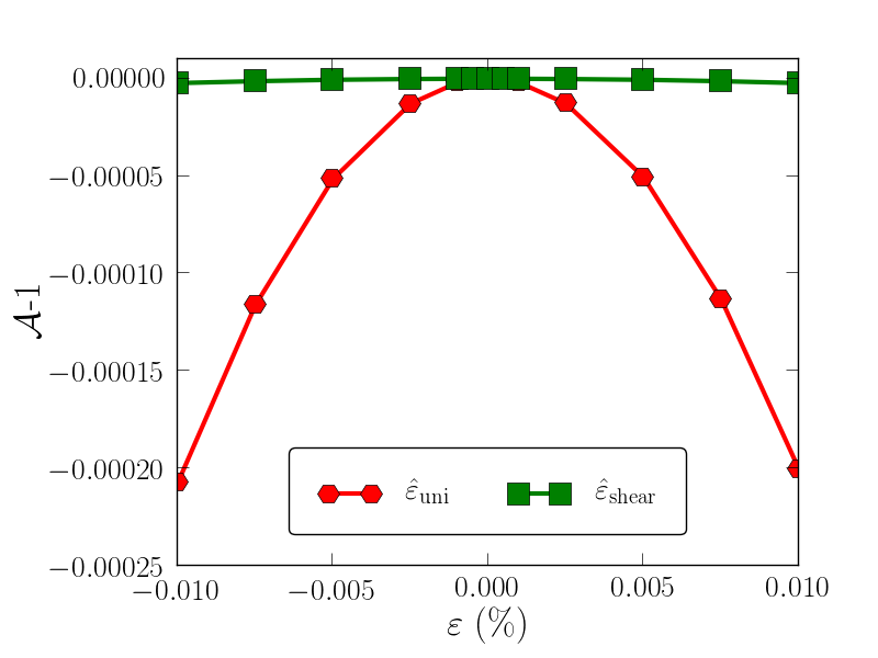
${\cal A}(\hat{\varepsilon})$ is plotted as a function of $\hat{\varepsilon}_{\rm hs}$, $\hat{\varepsilon}_{\rm uni}$, and $\hat{\varepsilon}_{\rm shear}$ in Fig. S4. ${\cal A}(\hat{\varepsilon})$ shows a quadratic behavior as a function of $\varepsilon_{\rm uni}$ and $\varepsilon_{\rm shear}$. It does, however, behave linearly as a function of $\varepsilon_{\rm hs}$. The trends at small $\varepsilon_{\parallel}<0$ evidenced in Fig. S3 can, therefore, be ascribed to the effects of hydrostatic strains on the hyperfine coupling constant. As a matter of fact, ${\cal A}(\varepsilon_{\parallel})={\cal A}(\hat{\varepsilon}_{\rm hs})+{\cal A}(\hat{\varepsilon}_{\rm uni}^{001})$ for uniaxial $[001]$ stress, and ${\cal A}(\varepsilon_{\parallel})={\cal A}(\hat{\varepsilon}_{\rm hs})+{\cal A}(\hat{\varepsilon}_{\rm uni}^{110})+{\cal A}(\hat{\varepsilon}_{\rm shear}^{110})$ for uniaxial $[110]$ stress, showing the relevance of this decomposition.

II.4 Discussion

Although not predicted by the valley repopulation model, the existence of a $\propto\varepsilon_{\rm hs}$ term in ${\cal A}$ is allowed by symmetries Pines et al. (1957). Indeed, a symmetry analysis suggests that, to second order in $\varepsilon_{ij}$:

$${\cal A}-1 =\frac{K}{3}(\varepsilon_{xx}+\varepsilon_{yy}+\varepsilon_{zz})$$

$$+L(\varepsilon_{xx}^{2}+\varepsilon_{yy}^{2}+\varepsilon_{zz}^{2})+M(\varepsilon_{yy}\varepsilon_{zz}+\varepsilon_{xx}\varepsilon_{zz}+\varepsilon_{xx}\varepsilon_{yy})+N(\varepsilon_{yz}^{2}+\varepsilon_{xz}^{2}+\varepsilon_{xy}^{2})\,,$$ (S12)

where $K=\partial{\cal A}/\partial\varepsilon_{\rm hs}$, $L$, $M$ and $N$ are constants. A fit to the tight-binding data yields:

$$K =29.3$$

$$L\simeq-M =-9064$$

$$N =-225$$ (S13)

Eq. (S12) then simplifies into:

$${\cal A}-1 =\frac{K}{3}(\varepsilon_{xx}+\varepsilon_{yy}+\varepsilon_{zz})$$

$$+\frac{L}{2}\left[(\varepsilon_{yy}-\varepsilon_{zz})^{2}+(\varepsilon_{xx}-\varepsilon_{zz})^{2}+(\varepsilon_{xx}-\varepsilon_{yy})^{2}\right]+N(\varepsilon_{yz}^{2}+\varepsilon_{xz}^{2}+\varepsilon_{xy}^{2})\,.$$ (S14)

We find $L\simeq-M$ because there is no sizable non-linearity in the dependence of ${\cal A}$ on hydrostatic strain in the investigated range $|\varepsilon_{\rm hs}|<10^{-4}$ (no $\propto\varepsilon_{\rm hs}^{2}$ term above when $\varepsilon_{xx}=\varepsilon_{yy}=\varepsilon_{zz}$). Also note that the effects of the quadratic shear terms are usually negligible with respect to the effects of the quadratic uniaxial terms ($N\ll L$).

The quadratic $L$ term is mostly due to the coupling of the $1s(A_{1})$ with the $1s(E)$ states of the impurity under uniaxial strain. The VRM of Ref. Wilson and Feher, 1961a actually suggests $L=-2\Xi_{u}^{2}/(9\Delta^{2})$, where $\Xi_{u}=8.6$ eV is the uniaxial deformation potential of the conduction band of silicon and $\Delta$ is the splitting between the $1s(A_{1})$ and the $1s(E)$ state. For Bi ($\Delta=41$ meV), the VRM predicts $L=-9720$, in close agreement with the TB data. The linear hydrostatic term is due, on the other hand, to the coupling of the $1s(A_{1})$ with $2s(A_{1})$ state (and possibly higher $s$ states with the same symmetry). This coupling results from the variations of the on-site correction on the bismuth impurity, and from the variations of the bismuth-silicon interactions under hydrostatic strain – in other words, from the variations of the depth and shape of the “central cell correction” Lipari et al. (1980) not accounted for by the VRM.

Indeed, the total potential on the bismuth atom catches contributions from the tails of the atomic potentials of the neighboring silicon atoms, and these contributions depend on the silicon-bismuth bond lengths. As a matter of fact, the present TB model includes a strain-dependent correction for the energy $E_{i\mu}$ of orbital $\mu\equiv s,p,d,s^{*}$ of atom $i$ Niquet et al. (2009):

$$E_{i\mu}=E_{i\mu}^{0}+\frac{3}{4}\alpha_{i\mu}\sum_{j\in{\rm NN}(i)}\frac{d_{ij}-d_{ij}^{0}}{d_{ij}^{0}}=E_{i\mu}^{0}+3\alpha_{i\mu}\varepsilon_{\rm hs}\,,$$ (S15)

where the sum runs over the nearest neighbors $j$ of atom $i$, $d_{ij}$ is the distance between atoms $i$ and $j$, and $d_{ij}^{0}$ is the relaxed bond length. $E_{i\mu}^{0}$ is the energy of the orbital in the reference, unstrained system and $\alpha_{i\mu}$ characterizes the deepening of the potential under strain. The interactions between bismuth and the nearest neighbor silicon atoms scale, on the other hand, as $(d_{ij}/d_{ij}^{0})^{n}$, with $n$ close to 2.

In the present TB model, the parameters $\alpha_{i\mu}$ and the exponents $n$ of bismuth are the same as for silicon. Although this choice is a safe first guess, it can only provide a semi-quantitative description of the dependence of ${\cal A}$ on hydrostatic strain. This is why the TB $K=29.3$ is significantly larger than the experimental $K=19.1$. We may, in the spirit of Eqs. (S2), lump all corrections to the TB model into the $\alpha_{i\mu}$. Therefore, we tentatively set:

$$\alpha_{i\mu}({\rm Bi})=\alpha_{i\mu}({\rm Si})+\Delta\alpha\,,$$ (S16)

and adjust $\Delta\alpha$ on the experimental $K$. This yields $\Delta\alpha=3.48$ eV for bismuth.

	Coulomb tail	$U_{s}=U_{s^{*}}$ (eV)	$U_{p}$ (eV)	$U_{d}$ (eV)	$\Delta\alpha$ (eV)	$K$	$L$	$N$
P	$-e^{2}/(\kappa R_{i})$	$4.535$	$2.405$	$2.055$	$-19.50$	$79.5$	-103640	1277
As	$-e^{2}/(\kappa R_{i})$	$5.060$	$2.330$	$0.325$	$-2.68$	$37.2$	-33836	833
Sb	Nara [Eq. (S1)]	$4.629$	$4.448$	$0.000$	$-2.54$	$32.6$	-104340	1420
Bi	Nara [Eq. (S1)]	$5.862$	$3.690$	$0.000$	$3.48$	$19.1$	-9064	-225

Table SI: Nature of the Coulomb tail, on-site corrections $U$ [Eq. (S2)] and $\Delta\alpha$ [Eq. (S16)], and value of $K$, $L$ and $N$ for P, As, Sb and Bi donors in silicon.

We have repeated the same procedure for P, As and Sb. We give in Table SI the on-site parameters $U_{s}=U_{s^{*}}$, $U_{p}$, $U_{d}$ and $\Delta\alpha$ of each impurity, as well as the values of $K$, $L$ and $N$. The model for P and As Diarra et al. (2007) is based on a simple Coulomb tail $V(R_{i})=-e^{2}/(\kappa R_{i})$ instead of Eq. (S1).

The dependence of the binding energy $E_{b}$ of As impurities on the hydrostatic pressure $P$ has been measured by Holland and Paul ($dE_{b}/dP\simeq-0.05$ meV/kbar) Holland and Paul (1962) and by Samara and Barnes ($dE_{b}/dP\simeq-0.1$ meV/kbar) Samara and Barnes (1987). The electron hence gets more loosely bound to the impurity under pressure (or equivalently under compressive hydrostatic strain). This is consistent with the decrease of the hyperfine coupling constant $A$ reported here ($K<0$). Samara and Barnes explain the decrease of $E_{b}$ under pressure by the variations of the effective masses and dielectric constant $\kappa$. We point out, though, that there is also a significant contribution from the variations of the central cell correction. The variations of effective masses and dielectric constant actually make little contribution to $K$. In the simplest effective mass approximation, the wave function of the electron bound to the donor is indeed $\Psi(\vec{r})=e^{-r/a_{B}}/(\sqrt{\pi}a_{B}^{3/2})$, where $a_{B}=\hbar^{2}\kappa/(m^{*}e^{2})$ is the Bohr radius. Hence, $|\Psi(\vec{0})|^{2}=1/(\pi a_{B}^{3})$, so that:

$$K=3\left(\frac{1}{m^{*}}\frac{\partial m^{*}}{\partial\varepsilon_{\rm hs}}-\frac{1}{\kappa}\frac{\partial\kappa}{\partial\varepsilon_{\rm hs}}\right)$$ (S17)

Ab-initio calculations within density functional theory (see next section) give $(1/\kappa)(\partial\kappa/\partial\varepsilon_{\rm hs})=0.78$, $(1/m^{*})(\partial m^{*}/\partial\varepsilon_{\rm hs})=-0.19$ for the longitudinal mass, and $(1/m^{*})(\partial m^{*}/\partial\varepsilon_{\rm hs})=1.54$ for the transverse mass. Therefore, the variations of the masses and dielectric constant are expected to have little net effect on the hyperfine coupling constant.

III Density functional theory calculations

In order to strengthen the above interpretation, we have also performed first principles calculations using density functional theory (DFT) with the Perdew-Burke-Ernzerhof (PBE) exchange-correlation functional Perdew et al. (1996) and the projector-augmented wave method Blöchl (1994) in the Vienna Ab-initio Simulation Package (VASP) Kresse and Furthmüller (1996), following the methodology described in Ref. Blöchl (2000). The calculations were carried out on one Bi impurity in a 1728-atom supercell, with a 250 eV plane-wave cutoff energy. DFT describes the central cell correction around the bismuth impurity from first principles and captures the atomic relaxations not accounted for by TB calculations — due to its accuracy in the immediate vicinity of the donor it could be expected to provide a good description of the variation of the hyperfine coupling with strains. Nevertheless, due to the finite size of the supercell, DFT misses the long range Coulomb tail of the potential Niquet et al. (2010), which (along with over-delocalization arising from the self-interaction error in PBE) contributes to an significant underestimation in the absolute value the hyperfine interaction (1102 MHz).

The ab-initio hyperfine coupling shows the expected linear dependence on hydrostatic strain over the entire range explored here (up to $\varepsilon_{xx}=\varepsilon_{yy}=\varepsilon_{zz}=2\times 10^{-3}$). We extract a coefficient $K=17.5$, in good agreement with the experimental data. The ab-initio quadratic term is $L=-1.17\times 10^{4}$, as obtained from a fit to the calculated data with $\varepsilon_{zz}\leq 10^{-3}$ and $\varepsilon_{xx}=\varepsilon_{yy}=0$. Deviations are observed for higher strains, consistent with the higher-order terms present in the VRM. The equilibrium bismuth-silicon bond length (2.651 Å) is significantly larger than the Si-Si bond length (2.367 Å in the bulk). All Bi-Si and Si-Si bonds are simply scaled by the hydrostatic strain, to within better than 0.001 Å.

These data provide further support for the linear dependence of the hyperfine parameter on the hydrostatic component of strain, and illustrate the complementary strengths of these two computational approaches (DFT and tight-binding) in modelling the behaviour of donors in silicon.

IV Modeling g-factor anisotropy

The ellipsoidal shape of the Si conduction band minima in $k$-space results in differing effective masses for Bloch waves parallel and perpendicular to the valley axis at these points Yu and Cardona (1999). This leads to a single-valley g-factor which is anisotropic, with $g_{\mu}^{2}=g_{\parallel}^{2}\cos^{2}\phi+g_{\perp}^{2}\sin^{2}\phi$, where $g_{\parallel}$ and $g_{\perp}$ are the g-factors parallel and perpendicular to the valley axis, and $\phi$ is the angle between the magnetic field and the valley axis. In the case of a donor, the g-factor is found by summing over the relative contribution from each valley such that $g_{\rm donor}=\sum_{\mu=1}^{6}\alpha_{\mu}^{2}g_{\mu}$. For the unstrained $1s(A_{1})$ donor ground state, which is an equal superposition of all six equivalent valleys, this summation leads to a cancellation of the anisotropy, leaving $g_{0}=\frac{1}{3}g_{\parallel}+\frac{2}{3}g_{\perp}$. Under strain, the valleys repopulate, breaking this cancellation symmetry. In our system with $\theta$ defined as in figure S1, the resulting g-factor anisotropy can be modeled using the VRM Wilson and Feher (1961b) by:

$$\left.\cfrac{\partial g}{\partial\epsilon_{11}}\right\rvert_{\textrm{VRM}}=\beta_{\textrm{VRM}}(3\cos^{2}\theta-1)$$ (S18)

where:

$$\beta_{\textrm{VRM}}=\cfrac{2\Xi_{u}}{9\Delta}(g_{\parallel}-g_{\perp})(k_{1}+k_{2})\,.$$ (S19)

$g_{\parallel}$ and $g_{\perp}$ are the parallel and perpendicular g-factors, $\Xi_{u}$ is the uniaxial deformation potential, $\Delta$ is the donor-dependent $1s(A_{1})$-$1s(E)$ splitting, and $k_{1}$ and $k_{2}$ are defined in Eq. S11.

It is also known that the g-factor of a single valley is changed in the presence of shear strain by the coupling with the opposite valley. Following Wilson & Feher Wilson and Feher (1961b), the effective Hamiltonian for this mechanism can be written YMN :

$$\mathcal{\hat{H}}_{\textrm{shear}}=C\mu_{B}\varepsilon_{xy}(B_{x}S_{y}+B_{y}S_{x})$$ (S20)

where $C$ is a coefficient involving spin-orbit coupling matrix elements Wilson and Feher (1961b). Rewriting the corresponding g-factor contribution in terms of $\varepsilon_{11}$ results in a second anisotropic term:

$$\left.\cfrac{\partial g}{\partial\epsilon_{11}}\right\rvert_{\textrm{shear}}=\beta_{\textrm{shear}}(3\cos^{2}\theta-3)$$ (S21)

where:

$$\beta_{\textrm{shear}}=\cfrac{C(1-k_{1})}{3}\,.$$ (S22)

Then, the derivative of the ESR transition frequency with respect to the uniaxial strain reads:

$$\cfrac{\textrm{d}f}{\textrm{d}\varepsilon_{11}}=\cfrac{\partial A}{\partial\varepsilon_{11}}\cfrac{\partial f}{\partial A}+\Bigg{[}\left.\cfrac{\partial g}{\partial\epsilon_{11}}\right\rvert_{\textrm{VRM}}+\left.\cfrac{\partial g}{\partial\epsilon_{11}}\right\rvert_{\textrm{shear}}\Bigg{]}\cfrac{\partial f}{\partial g}\,.$$ (S23)

$\partial f/\partial g$ can be calculated for each transition in the same manner as $\partial f/\partial A$ by solving the spin Hamiltonian while varying the value of g. We use a linear least squares regression to fit this model to the experimental data. We introduce three fitting parameters characterising the strength of the different effects for each donor: $K=\partial(A/A_{0})/\partial\epsilon_{\rm hs}$, $\beta_{\textrm{VRM}}$ and $\beta_{\textrm{shear}}$. The results of these fits are reported in table SII and figure 4 in the main text for Si:Sb, Si:As, and Si:P. The absence of a clear anisotropy for Si:Bi could be explained by the relatively small magnitude of the predicted g-factor effects in comparison with the absolute shifts due to the modified hyperfine interaction.

Donor	$K=\frac{\partial(A/A_{0})}{\partial\epsilon_{\rm hs}}$ (exp.)	$\beta_{\textrm{VRM}}\times 10^{-3}$ (theory)	$\beta_{\textrm{VRM}}\times 10^{-3}$ (exp.)	$\beta_{\textrm{shear}}\times 10^{-3}$ (theory)	$\beta_{\textrm{shear}}\times 10^{-3}$ (exp.)
31P	$79.2\pm 25.7$	$126.7$	$206\pm 51$	$78$	$173\pm 33$
75As	$37.4\pm 3.3$	$77.5$	$165.1\pm 24.6$	$78$	$96\pm 15.6$
121Sb	$32.8\pm 2.3$	$146.0$	$197.6\pm 25.8$	$78$	$90.3\pm 16.4$
209Bi	$19.1\pm 0.3$	$42.5$	-	$78$	-

Table SII: Parameters $K=\partial(A/A_{0})/\partial\epsilon_{\rm hs}$, $\beta_{\textrm{VRM}}$ and $\beta_{\textrm{shear}}$ extracted from the experimental data, along with theoretical values for $\beta_{\textrm{VRM}}$ and $\beta_{\textrm{shear}}$. The theoretical values are calculated using $C=0.44$ Wilson and Feher (1961b), $\Delta$ values from Ref. Ramdas and Rodriguez, 1981, and $(g_{\parallel}-g_{\perp})$ values from Ref. Wilson and Feher (1961b). We assume $(g_{\parallel}-g_{\perp})\approx 1.1\times 10^{-3}$ for Si:Bi.

We compare the extracted parameters with theoretical predictions for $\beta_{\textrm{VRM}}$ and $\beta_{\textrm{shear}}$ [Eqs. (S19) and (S22)] calculated using $C=0.44$ Wilson and Feher (1961b), $\Delta$ values from Ref. Ramdas and Rodriguez, 1981, and $g_{\parallel}-g_{\perp}$ values from Ref. Wilson and Feher (1961b). The measured strengths of the g-factor effects agree with theory within approximately a factor of 2. Tight binding simulations with the present model (see also Ref. Rahman et al., 2009) predict that the very small $g_{\parallel}-g_{\perp}$ is approximately an order of magnitude larger than given by Ref. Wilson and Feher (1961b). It is interesting to note that the experimental data sit between Ref. Wilson and Feher (1961b) and the TB predictions.

V Full Experimental dataset for all donors

Figure S5: Full dataset for Si:Bi showing frequency shifts for all ten ESR transitions as a function of strain $\varepsilon_{11}$ and $\theta$. Linear fits are shown for each transition.

Figure S6: Full dataset for Si:Sb showing frequency shifts for all six ESR transitions as a function of strain $\varepsilon_{11}$ and $\theta$. Linear fits are shown for each transition.

Figure S7: Full dataset for Si:As showing frequency shifts for all four ESR transitions as a function of strain $\varepsilon_{11}$ and $\theta$. Linear fits are shown for each transition.

Figure S8: Full dataset for Si:P showing frequency shifts for both ESR transitions as a function of strain $\varepsilon_{11}$ and $\theta$. Linear fits are shown for each transition.

References

- Tyryshkin et al. (2011) A. M. Tyryshkin, S. Tojo, J. J. L. Morton, H. Riemann, N. V. Abrosimov, P. Becker, H.-J. Pohl, T. Schenkel, M. L. W. Thewalt, and K. M. Itoh, Nature Materials 11, 143 (2011).
- Saeedi et al. (2013) K. Saeedi, S. Simmons, J. Z. Salvail, P. Dluhy, H. Riemann, N. V. Abrosimov, P. Becker, H.-J. Pohl, J. J. L. Morton, and M. L. W. Thewalt, Science 342, 830 (2013).
- Pla et al. (2013) J. J. Pla, K. Y. Tan, J. P. Dehollain, W. H. Lim, J. J. L. Morton, F. A. Zwanenburg, D. N. Jamieson, A. S. Dzurak, and A. Morello, Nature 496, 334 (2013).
- Muhonen et al. (2015) J. T. Muhonen, A. Laucht, S. Simmons, J. P. Dehollain, R. Kalra, F. E. Hudson, S. Freer, K. M. Itoh, D. N. Jamieson, and J. C. Mccallum, Journal of Physics: Condensed Matter 27, 154205 (2015).
- Kane (1998) B. E. Kane, Nature 393, 133 (1998).
- O’Brien et al. (2001) J. L. O’Brien, S. R. Schofield, M. Y. Simmons, R. G. Clark, A. S. Dzurak, N. J. Curson, B. E. Kane, N. S. McAlpine, M. E. Hawley, and G. W. Brown, Physical Review B 64, 161401 (2001).
- Tyryshkin et al. (2003) A. M. Tyryshkin, S. A. Lyon, A. V. Astashkin, and A. M. Raitsimring, Physical Review B 68, 193207 (2003).
- Stegner et al. (2006) A. R. Stegner, C. Boehme, H. Huebl, M. Stutzmann, K. Lips, and M. S. Brandt, Nature Physics 2, 835 (2006).
- Morton et al. (2008) J. J. L. Morton, A. M. Tyryshkin, R. M. Brown, S. Shankar, B. W. Lovett, A. Ardavan, T. Schenkel, E. E. Haller, J. W. Ager, and S. A. Lyon, Nature 455, 1085 (2008).
- Simmons et al. (2011) S. Simmons, R. M. Brown, H. Riemann, N. V. Abrosimov, P. Becker, H.-J. Pohl, M. L. W. Thewalt, K. M. Itoh, and J. J. L. Morton, Nature 470, 69 (2011).
- Fuechsle et al. (2012) M. Fuechsle, J. A. Miwa, S. Mahapatra, H. Ryu, S. Lee, O. Warschkow, L. C. L. Hollenberg, G. Klimeck, and M. Y. Simmons, Nature Nanotechnology 7, 242 (2012).
- Büch et al. (2013) H. Büch, S. Mahapatra, R. Rahman, A. Morello, and M. Y. Simmons, Nature Communications 4 (2013), 10.1038/ncomms3017.
- Franke et al. (2015) D. P. Franke, F. M. Hrubesch, M. Künzl, H.-W. Becker, K. M. Itoh, M. Stutzmann, F. Hoehne, L. Dreher, and M. S. Brandt, Physical Review Letters 115, 057601 (2015).
- Franke et al. (2016) D. P. Franke, M. P. D. Pflüger, P.-A. Mortemousque, K. M. Itoh, and M. S. Brandt, Physical Review B 93, 161303 (2016).
- Wolfowicz et al. (2014) G. Wolfowicz, M. Urdampilleta, M. L. W. Thewalt, H. Riemann, N. V. Abrosimov, P. Becker, H.-J. Pohl, and J. J. L. Morton, Physical Review Letters 113, 157601 (2014).
- Singh et al. (2016) M. Singh, J. L. Pacheco, D. Perry, E. Garratt, G. T. Eyck, N. C. Bishop, J. R. Wendt, R. P. Manginell, J. Dominguez, and T. Pluym, Applied Physics Letters 108, 062101 (2016).
- Morley et al. (2010) G. W. Morley, M. Warner, A. M. Stoneham, P. T. Greenland, J. V. Tol, C. W. M. Kay, and G. Aeppli, Nature Materials 9, 725 (2010).
- Mortemousque et al. (2014) P. A. Mortemousque, S. Berger, T. Sekiguchi, C. Culan, R. G. Elliman, and K. M. Itoh, Physical Review B 89, 155202 (2014).
- Saeedi et al. (2015) K. Saeedi, M. Szech, P. Dluhy, J. Salvail, K. Morse, H. Riemann, N. Abrosimov, N. Nötzel, K. Litvinenko, B. Murdin, and M. Thewalt, Scientific Reports 5 (2015), 10.1038/srep10493.
- Wolfowicz et al. (2013) G. Wolfowicz, A. M. Tyryshkin, R. E. George, H. Riemann, N. V. Abrosimov, P. Becker, H.-J. Pohl, M. L. W. Thewalt, S. A. Lyon, and J. J. L. Morton, Nature Nanotechnology 8, 881 (2013).
- Morello et al. (2010) A. Morello, J. J. Pla, F. A. Zwanenburg, K. W. Chan, K. Y. Tan, H. Huebl, M. Möttönen, C. D. Nugroho, C. Yang, J. A. van Donkelaar, A. D. Alves, D. N. Jamieson, C. C. Escott, L. C. L. Hollenberg, R. G. Clark, and A. S. Dzurak, Nature 467, 687 (2010).
- Pla et al. (2012) J. J. Pla, K. Y. Tan, J. P. Dehollain, W. H. Lim, J. J. L. Morton, D. N. Jamieson, A. S. Dzurak, and A. Morello, Nature 489, 541 (2012).
- Bienfait et al. (2016) A. Bienfait, J. J. Pla, Y. Kubo, X. Zhou, M. Stern, C. C. Lo, C. D. Weis, T. Schenkel, D. Vion, D. Esteve, J. Morton, and P. Bertet, Nature 531, 74 (2016).
- Eichler et al. (2017) C. Eichler, A. J. Sigillito, S. A. Lyon, and J. R. Petta, Physical Review Letters 118, 037701 (2017).
- Zollitsch et al. (2015) C. W. Zollitsch, K. Mueller, D. P. Franke, S. T. B. Goennenwein, M. S. Brandt, R. Gross, and H. Huebl, Applied Physics Letters 107, 142105 (2015).
- Angus et al. (2007) S. J. Angus, A. J. Ferguson, A. S. Dzurak, and R. G. Clark, Nano Letters 7, 2051 (2007).
- Bruno et al. (2015) A. Bruno, G. D. Lange, S. Asaad, K. L. V. D. Enden, N. K. Langford, and L. Dicarlo, Applied Physics Letters 106, 182601 (2015).
- Lyon et al. (1977) K. G. Lyon, G. L. Salinger, C. A. Swenson, and G. K. White, Journal of Applied Physics 48, 865 (1977).
- Swenson (1983) C. A. Swenson, Journal of Physical and Chemical Reference Data 12, 179 (1983).
- Roberts (1982) R. B. Roberts, Journal of Physics D: Applied Physics 15 (1982), 10.1088/0022-3727/15/9/004.
- NIS (1991) NIST Standard Reference Material 739, Certificate (1991).
- Nix and Macnair (1941) F. C. Nix and D. Macnair, Physical Review 60, 597 (1941).
- Morello et al. (2009) A. Morello, C. C. Escott, H. Huebl, L. H. Willems van Beveren, L. C. L. Hollenberg, D. N. Jamieson, A. S. Dzurak, and R. G. Clark, Physical Review B 80, 081307 (2009).
- Pla et al. (2016) J. J. Pla, A. Bienfait, G. Pica, J. Mansir, F. A. Mohiyaddin, A. Morello, T. Schenkel, B. W. Lovett, J. J. L. Morton, and P. Bertet, “Strain-induced nuclear quadrupole splittings in silicon devices,” (2016), arXiv:1608.07346 .
- Bardeen and Shockley (1950) J. Bardeen and W. Shockley, Physical Review 80, 72 (1950).
- Herring and Vogt (1957) C. Herring and E. Vogt, Physical Review 105, 1933 (1957).
- Thorbeck and Zimmerman (2015) T. Thorbeck and N. M. Zimmerman, AIP Advances 5, 087107 (2015).
- Veldhorst et al. (2015) M. Veldhorst, C. H. Yang, J. C. C. Hwang, W. Huang, J. P. Dehollain, J. T. Muhonen, S. Simmons, A. Laucht, F. E. Hudson, and K. M. Itoh, Nature 526, 410 (2015).
- Wilson and Feher (1961a) D. K. Wilson and G. Feher, Physical Review 124, 1068 (1961a).
- Huebl et al. (2006) H. Huebl, A. R. Stegner, M. Stutzmann, M. S. Brandt, G. Vogg, F. Bensch, E. Rauls, and U. Gerstmann, Phys. Rev. Lett. 97, 166402 (2006).
- Dreher et al. (2011) L. Dreher, T. A. Hilker, A. Brandlmaier, S. T. B. Goennenwein, H. Huebl, M. Stutzmann, and M. S. Brandt, Physical Review Letters 106, 037601 (2011).
- Pines et al. (1957) D. Pines, J. Bardeen, and C. P. Slichter, Phys. Rev. 106, 489 (1957).
- Schweiger and Jeschke (2005) A. Schweiger and G. Jeschke, Principles of pulse electron paramagnetic resonance (Oxford University Press, 2005).
- (44) See Supplemental Material for further details on experimental methods, tight-binding modeling, DFT calculations, modeling the g-factor anisotropy, and complete datasets. .
- Zhang et al. (2014) L. Zhang, R. Barrett, P. Cloetens, C. Detlefs, and M. S. D. Rio, Journal of Synchrotron Radiation 21, 507 (2014).
- Ross (2017) P. Ross, Ph.D. thesis, University College London (2017).
- Hahn (1950) E. L. Hahn, Physical Review 80, 580 (1950).
- Kohn and Luttinger (1955) W. Kohn and J. M. Luttinger, Physical Review 98, 915 (1955).
- Luttinger and Kohn (1955) J. M. Luttinger and W. Kohn, Physical Review 97, 869 (1955).
- Pantelides and Sah (1974) S. T. Pantelides and C. T. Sah, Physical Review B 10, 621 (1974).
- Pica et al. (2014a) G. Pica, G. Wolfowicz, M. Urdampilleta, M. L. W. Thewalt, H. Riemann, N. V. Abrosimov, P. Becker, H.-J. Pohl, J. J. L. Morton, R. N. Bhatt, S. A. Lyon, and B. W. Lovett, Physical Review B 90, 195204 (2014a).
- Pica et al. (2014b) G. Pica, B. W. Lovett, R. N. Bhatt, and S. A. Lyon, Physical Review B 89, 235306 (2014b).
- Niquet et al. (2009) Y. M. Niquet, D. Rideau, C. Tavernier, H. Jaouen, and X. Blase, Physical Review B 79, 245201 (2009).
- Roche et al. (2012) B. Roche, E. Dupont-Ferrier, B. Voisin, M. Cobian, X. Jehl, R. Wacquez, M. Vinet, Y.-M. Niquet, and M. Sanquer, Physical Review Letters 108, 206812 (2012).
- Usman et al. (2015) M. Usman, R. Rahman, J. Salfi, J. Bocquel, B. Voisin, S. Rogge, G. Klimeck, and L. L. C. Hollenberg, Journal of Physics: Condensed Matter 27, 154207 (2015).
- Nara and Morita (1966) H. Nara and A. Morita, Journal of the Physical Society of Japan 21, 1852 (1966).
- Bernholc and Pantelides (1977) J. Bernholc and S. T. Pantelides, Physical Review B 15, 4935 (1977).
- Krag et al. (1970) W. E. Krag, W. H. Kleiner, and H. J. Zieger, in Proceedings of the 10th International Conference on the Physics of Semiconductors (Cambridge, Massachusetts, 1970), edited by S. P. Keller, J. C. Hensel, and F. Stern (USAEC Division of Technical Information, Washington D.C., 1970) p. 271.
- Ramdas and Rodriguez (1981) A. K. Ramdas and S. Rodriguez, Reports on Progress in Physics 44, 1297 (1981).
- Zhukavin et al. (2011) R. K. Zhukavin, K. A. Kovalevsky, V. V. Tsyplenkov, V. N. Shastin, S. G. Pavlov, H.-W. Hübers, H. Riemann, N. V. Abrosimov, and A. K. Ramdas, Applied Physics Letters 99, 171108 (2011).
- Lipari et al. (1980) N. Lipari, A. Baldereschi, and M. Thewalt, Solid State Communications 33, 277 (1980).
- Diarra et al. (2007) M. Diarra, Y.-M. Niquet, C. Delerue, and G. Allan, Physical Review B 75, 045301 (2007).
- Holland and Paul (1962) M. G. Holland and W. Paul, Physical Review 128, 30-38 (1962).
- Samara and Barnes (1987) G. A. Samara and C. E. Barnes, Physical Review B 35, 7575 (1987).
- Perdew et al. (1996) J. P. Perdew, K. Burke, and M. Ernzerhof, Phys. Rev. Lett. 77, 3865 (1996).
- Blöchl (1994) P. E. Blöchl, Phys. Rev. B 50, 17953 (1994).
- Kresse and Furthmüller (1996) G. Kresse and J. Furthmüller, Phys. Rev. B 54, 11169 (1996).
- Blöchl (2000) P. E. Blöchl, Phys. Rev. B 62, 6158 (2000).
- Niquet et al. (2010) Y. M. Niquet, L. Genovese, C. Delerue, and T. Deutsch, Physical Review B 81, 161301 (2010).
- Yu and Cardona (1999) P. Y. Yu and M. Cardona, Fundamentals of semiconductors: physics and materials properties (Springer, 1999).
- Wilson and Feher (1961b) D. K. Wilson and G. Feher, Physical Review 124, 1068 (1961b).
- (23) The form of Eq. (9) of Ref. Wilson and Feher (1961b) suggests that in Ref. Wilson and Feher (1961b) is the “engineering” shear strain , hence the factor 2 difference between Eq. (S20) and Eq. (8) of Ref. Wilson and Feher (1961b).
- Rahman et al. (2009) R. Rahman, S. H. Park, T. B. Boykin, G. Klimeck, S. Rogge, and L. C. L. Hollenberg, Physical Review B 80, 155301 (2009).