Abstract

This work is about Bohmian mechanics, a non-relativistic quantum theory about the motion of particles and their trajectories, named after its inventor David Bohm (Bohm,1952). This mechanics resolves all paradoxes associated with the measurement problem in nonrelativistic quantum mechanics. It accounts for quantum randomness, absolute uncertainty, the meaning of the wave function of a system, collapse of the wave function, and familiar (macroscopic) reality. We review the purpose for which Bohmian trajectories were invented: to serve as the foundation of quantum mechanics, i.e., to explain quantum mechanics in terms of a theory that is free of paradoxes and allows an understanding that is as clear as that of classical mechanics. To achieve this we analyse an optical interferometry experiment devised and carried out 2005 by Shahriar Afshar (Afshar,2005). The radical claim of Afshar implies in his own words the ‘observation of physical reality in the classical sense’ for both ‘which path (particle-like)’ and ‘interference (wave-like)’ properties of photons in the same experimental setup through the violation of the Englert-Greenberger duality relation (Englert,1996) that according to Englert can be regarded as quantifying of the ‘principle of complementarity’.

1 Introduction

“What exactly qualifies some physical systems to play the role of ‘measurer’? Was the wavefunction of the world waiting to jump for thousands of millions of years until a single-celled living creature appeared? Or did it have to wait a little longer, for some better qualified system… with a PhD? If the theory is to apply to anything but highly idealised laboratory operations, are we not obliged to admit that more or less ‘measurement-like’ processes are going on more or less all the time, more or less everywhere? Do we not have jumping then all the time?” Bel90 Bell

The classical ideal of passive measurements which simply reveal a preexisting reality cannot be sustained when we come to a quantum treatment of the measurement problem. In crude terms, one may say that at the quantum level the probe becomes as significant as the probed so one cannot ‘calculate away’ its influence to leave pure information regarding preexisting properties of an object. Because these interactions entail transformation of the object that only in special cases reveal the values of properties without altering them, has been suggested by Bell the continued use of the word ‘measurement’ in this context is liable to fuel misconceptions.

In short, Bell argued that the separation between the quantum system and the measuring apparatus is arbitrary. The encapsulation of the rest of the world (except the quantum system) into a mathematical entity called an operator $\hat{G}$, is a very clever trick that allows for straightforward calculations of the results of quantum measurements without considering the rest of the world.

In addition to the word ‘measurement’ we have the list of words: ‘system’, ‘apparatus’, ‘environment’, all this immediately imply an artificial division of the world, and an intention to neglect, or take only schematic account of, the interaction across the split. The notions of ‘microscopic’ and ‘macroscopic’ defy precise definition. So also do the notions of ‘reversible’ and ‘irreversible’. Einstein said that it is theory which decides what is ‘observable’. We think he was right, and if someone says ‘observation’ our answer is: Observation of what?.

If one accepts this arbitrary division of the world and that the usual quantum mechanical description of the state of a quantum system is indeed the complete description of that system, it seems hard to avoid the conclusion that quantum measurements typically fail to have results. Pointers on measurement devices typically fail to point, computer printouts typically fail to have anything definite written on them, and so on. More generally, macroscopic states of affairs tend to be grotesquely indefinite, with cats seemingly both dead and alive at the same time, and the like. This is not good!. These difficulties can be largely avoided by invoking the measurement axioms of quantum theory, in particular the collapse postulate, but doing so comes at a price. One then has to accept that quantum theory involves special rules for what happens during a measurement, rules that are in addition to, and not derivable from, the quantum rules governing all other situations.

We believe, however, that the measurement problem, as important as it is, is nonetheless but a manifestation of a more basic difficulty with standard quantum mechanics: it is not at all clear what quantum theory is about. Indeed, it is not at all clear what quantum theory actually says and with what does the quantum mechanics actually deal ?, Is quantum mechanics fundamentally about measurement and observation? Is it about the behavior of macroscopic variables? Or is it about our mental states? Is it about the behavior of wave functions? Or is it about the behavior of suitable fundamental microscopic entities, elementary particles and/or fields? Quantum mechanics provides us with formulas for lots of probabilities. What are these the probabilities of? Of results of measurements? Or are they the probabilities for certain unknown details about the state of a system, details that exist and are meaningful prior to measurement?

It is often said that such questions are the concern of the foundations of quantum mechanics, or of the interpretation of quantum mechanics but not. The problem is not about a philosophical discussion. Philosophy needs physics but physics needs no philosophy. Physics must be about the objective reality and need recognizes instead that a quantum theory must describe such a reality. We need an objective quantum description of nature. We need quantum physics without quantum philosophy.

This work revolves around an optical interferometry experiment that is a variation of the Young’s experiment. The experiment was devised and carried out in 2005 by Shahriar Afshar. Much has been written about this experiment, and from the point of view of the orthodox interpretation of quantum mechanics a satisfactory interpretation of the results could not be found. Supporters and critics of the Afshar’s interpretation of his results have concentrated on justify or refute the violation of the Englert-Greenberger duality relation reaching sharply divergent conclusions mutually incompatible and contradictory.

This work is only another example that confirms the fact that quantum mechanics, as Bell quite rightly said, is “unprofessionally vague and ambiguous.”. What is usually regarded as a fundamental problem in the foundations of quantum mechanics, a problem often described as that of interpreting quantum mechanics, is, we believe, better described as the problem of finding a sufficiently precise formulation of quantum mechanics, of finding a version of quantum mechanics that, while expressed in precise mathematical terms, is also clear as physics. In this work we show with the particular analisys of the Afshar’s experiment ‘paradox’ that Bohmian mechanics provides such a precise formulation.

2 Afshar’s experiment

The Afshar’s experiment Afs05  uses a setup similar to that for the double-slit experiment. The aim of the experiment is give information about ‘which-path’ a particle takes through the apparatus and the contrast or visibility of the interference pattern (IP) as the quantification of the ‘wave nature of the particle’. Afshar claimed that the experiment violates the Englert-Greenberger relation:

$$K^{2}+V^{2}\leq 1$$ (1)

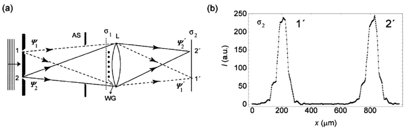
Figure 1: (a) Schematics of the Afshar’s setup. Laser light impinges upon a dual pinhole and two diffracted beams $\psi_{1}$ and $\psi_{2}$ emerge. The beams are apodized by an aperture stop (AS) and pass through the wire grid (WG) and the converging lens ($L$) to produce the irradiance profile in the photosensitive surface ($\sigma_{2}$). (b) Irradiance profile of the images at $\sigma_{2}$, while the WG is present. The irradiance ($I$) is measured in arbitrary units (a.u.) of grey-level intensity Afs05 .

That according to Englert Eng96 can be regarded as quantifying the notion of ‘wave-particle duality’ refers to the ‘principle of complementarity’ Bohr28 . The stages of the experiment are:

In stage (i) of the experiment the wire grid (WG) is not present. In this stage only one slit is left open, therefore, only the corresponding detector gets illuminated. Opening of the other slit (and illuminating the other detector simultaneously) does not change the image at the first detector.

In stage (ii) the setup is modified by inserting the WG directly in front of the lens ($L$). The WG is carefully positioned in such a way that the wires sit at the minima of the IP (which can be checked by inserting a screen at the position of WG and opening the second slit). It is then observed that if one of the two slits is blocked the image of the remaining open slit is strongly modified due to the presence of the grid. The wires of the grid reflect (and diffract) some of the photons, which leads to a reduction of the intensity and introduces the formation of stripes in the image of the slit.

In stage (iii) the other slit (previously blocked) is reopened (see Fig.1). The crucial result at this stage is that only a slight reduction in peak intensity is observed at detectors $C_{1}$ and $C_{2}$ to those obtained in the absence of the WG in stage (i).

The experiment has been repeated and its results have been confirmed, concluding that the fraction of photons that are stopped by the WG is maximally $1\%$ AFMK07 . But its interpretation is controversial, and some disagree that it violates (1), while also disagreeing amongst themselves as to why.

3 The orthodox origin of the Afhsar’s paradox

“Bohr’s principle of complementarity states that quantum systems (“quantons” for short) possess properties that are equally real but mutually exclusive. The best known example is what is colloquially termed wave-particle duality. In a loose manner of speaking it is sometimes phrased similarly to the following: Depending on the experimental situation a quanton behaves either like a particle or like a wave” Eng96 Englert

The radical claim of Afshar Afs05 implies in his own words the ‘observation of physical reality in the classical sense’ for both ‘which-path (particle-like)’ and ‘interference (wave-like)’ properties of photons in the same experimental setup. His claim of a violation of the inequality (1) that according to Englert can be regarded as quantifying the notion of ‘complementarity’ in wave-particle duality has produced strong criticism Kas05 ; Dre05 ; Kas09 ; Ste07 ; Jac08 ; Rei08 ; Qur10 ; Dre11 ; Qur12 . Researchers seeking a ‘resolution of the paradoxical findings’ have resorted to discredit the validity of Afshar’s analysis while also disagreeing amongst themselves as to why. Below is a brief summary of the papers about the Afshar’s experiment:

Some authors have tried to argue along the following line. Blocking dark fringes also blocks out parts of the bright fringes Jac08 ; Ste07 . Is that positioning the WG at the dark fringe locations is not enough to reveal the existence of the IP, without inducing any further perturbation on the transmitted light field. This because the WG has an unavoidable effect due to diffraction, which redirects some light from one ‘PATH’ to the wrong detector. The introduction of the grid has then according to they partially erased the ‘which-path’ information since it becomes impossible to univocally associate each output detector to a given path of the interferometer. They believe, when both slits are open, the photons contain full ‘which-path’, which is partially destroyed by partially blocking the bright fringes. They argue that since without the wires completely blocking the dark fringe, one cannot infer the existence of the interference, when one tries to increase the information about the existence of the interference, the ‘which-path’ is proportionately decreased. In Flo08 These kind of works have been criticized since assume the presence of an ideal IP at the WG and then shows using different experimental situations that the measure of the contrast of the IP is not possible.

Have been noticed in Qur12 that in these works, the calculation use as argument the theoretical existence of full interference, without any blocking wires. But without the blocking wires, the photons are claimed to have full ‘which-path’ (‘distinguishability = 1’ in their language). So, if one were to take their calculation of ‘distinguishablity’ as correct, then the existence of full interference in the calculation (in the sense of $|\psi|^{2}$ yielding an IP) seems to imply that quantum formalism allows existence of ‘interference’ for photons for which full ‘which-path’ exists.

Other authors Kas05 ; Kas09 ; Rei08 argues that the ‘COLLAPSE of the wave function’ TAKES PLACE after the fully articulated ‘interference’ (the IP is lost DOWNSTREAM from the ‘which-path’ measurement) has been indirectly indicated to exist by the fact that the grid does not significantly diminish the intensity of the final detection. But for these authors the latter measurement doesn’t give any physically meaningful ‘which-path’ information since the particle already ‘went through both slits’ and it would not be correct to say that the ‘which-path’ measurement indicates that the particle ‘actually went through’ only one or the other slit. The use of different kinds of setup in these works has been criticized in FK07 .

Finally in Dre05 ; Dre11 is said that the real problem in Afshar’s interpretation comes from the fact that the IP is not actually completely recorded because to prove experimentally that such sinusoidal IP actually exists is necessary record photons in the rest of the wires plane. In Qur10 ; Qur12 , is argues that the calculation of ‘distinguishability’ in Jac08 ; Ste07 is fundamentally flawed. This because if the ‘state of a particle’ is such that the modulus square of the wave function yields an IP ( and considering that in this experimental situation the existence of IP is established without actually disturbing the photons in any way, unlike Dre05 ; Dre11 ), then it the detectors detecting the photons behind the converging lens, do not yield any ‘which-path’ information. This because according to this author ‘MERE EXISTENCE of ‘which-path’ information in the state’ is sufficient to ‘DESTROY any POTENTIAL interference’.

The discussion in this section serves to understand only one thing, the fact that quantum mechanics, as Bell quite rightly said, is “unprofessionally vague and ambiguous”, and that only can produce an immense sea of confusion. This sea of confusion in this case is composed by the dozens of papers that try to prevent the violation of the mystic concept of ‘complementarity’, ‘complementarity’ is only food for mysticism and only leads to the belief that the laws of quantum mechanics are a Delphic oracle, which apparently require high priests to be deciphered, try of understand what ‘complementarity’ is or even worse defend it, is insane. Only one thing is and can be of course clear about this discussion and is that defend ‘complementarity’ is defend that the basic properties of matter can never be understood rationally in terms of unique and unambiguous models, implies that the use of complementary pairs of imprecisely defined concepts will be necessary for the detailed treatment of every domain that will ever be investigated. Thus, the limitations on our concepts implicit in the ‘principle of complementarity’ are regarded as absolute and final.

When we said that rational description of nature is possible, we mean that decoherence does not create the facts of our world, but rather produces a sequence of redundancies, which physically increase or stabilize decoherence. So the cat decoheres the atom, the observer decoheres the cat that decoheres the atom, the environment of the observer decoheres the observer that decoheres the cat that decoheres the atom and so on. In short, what needs to be described by the physical theory is the behavior of real objects, located in physical space, which account for the facts.

Try to refute Afshar’s claim to have shown a violation of ‘complementarity’ by arguing (using the language of all the previous works) that the ‘which-path’ information is partially erased or that the contrast of the IP is quite low, tacitly accepts the notion that (1) is applicable and assume that (1) have some relation with the concept of ‘complementarity’. Since Englert makes no mistakes in computation, the first and consequent question is, whether (1) applies to the Afshar’s experiment. In the next chapters is presented a brief introduction to Bohmian mechanics  and then is showed from the Bohmian explanation of the measurement process how this answer can be trivially answered without any reference to ‘complementarity’.

4 Bohmian mechanics

Bohmian mechanics  or more exactly ‘de Broglie-Bohm theory’, is a realistic, non-relativistic quantum theory about moving particles. The Bohmian and the orthodox descriptions of a measurement produce the same probabilistic predictions. However, the mathematical implementation of the equations of motion in each case is quite different. The Bohmian time evolution of the total wave function and the total trajectory is all we need to explain any quantum process, including the orthodox measurement process. The orthodox quantum theory requires an operator to describe the effect of the measuring apparatus, but this operator is not needed in the Bohmian description of a quantum system of $N$ particles. Here, its state is given by variables DS09 :

$$(Q\,,\,\psi)\ ,$$

where $Q=({\bf Q}_{1}\dots\bf Q_{N})\in\mbox{${\rm I\!R}$}^{3N},$ with ${\bf Q}_{k}$ being the positions of particles, and $\psi=\psi(q)=\psi({\bf q}_{1}\dots\bf q_{N})$ denoting the wave function.

We already have an evolution equation for $\psi$, i.e., Schrödinger’s equation DS09 :

$$i\hbar\frac{\partial\psi}{\partial t}=-{\sum}_{k=1}^{N}\frac{{\hbar}^{2}}{2m_{k}}\Delta_{k}\psi+V\psi\ ,$$ (2)

the evolution equation for $Q$ is of the form DS09 :

$$\frac{dQ}{dt}=v^{\psi}(Q)\ ,$$ (3)

where $v^{\psi}=({\bf v}^{\psi}_{1}\dots\bf v^{\psi}_{N})$. Thus, the role of $\psi$ is to ‘choreograph’ a motion of particles through the vector field on the configuration space that it defines. By imposing space-time symmetry—Galilean and time-reversal invariance (or covariance), and ‘simplicity’, we obtain for a general $N-$particle system DS09 :

$${\bf v}_{k}^{\psi}=\frac{\hbar}{m_{k}}{\rm Im}\frac{\mbox{\boldmath$\nabla$\unboldmath}_{k}\psi}{\psi}\ .$$ (4)

The wave function affects the behavior of the configuration, i.e., of the particles. This is expressed by (4), but in Bohmian mechanics there’s no back action, no effect in the other direction, of the configuration upon the wave function, which evolves autonomously via (2) in which the actual configuration $Q$ does not appear, also for a multi-particle system the wave function  $\psi=\psi(q)=\psi({\bf q}_{1}\dots\bf q_{N})$ is not a weird field on physical space, its a weird field on configuration space, the set of all hypothetical configurations of the system. What it suggests to us is that you should think of the wave function as describing a law and not as some sort of concrete physical reality, we want to suggest one should think about is the possibility that it’s nomological DGN13 , nomic-that it’s really more in the nature of a law than a concrete physical reality.

To connect this theory with the particle mechanics we already know (Newtonian mechanics), we write the wave function  in the form $\psi=R\exp[iS/\hbar]$, where $R$ and $S$ are real. Then the Schrödinger’s equation reduces to the following two equations DS09 :

$$\frac{\partial S}{\partial t}+\frac{{(\mbox{\boldmath$\nabla$\unboldmath}S)}^{2}}{2m}+V+Q=0\ ,$$ (5)

where $V$ and $Q$ denote classical and quantum potential respectively, such that:

$$Q=-\frac{\hbar^{2}}{2m}\frac{\Delta R}{R}\ ,$$ (6)

and

$$\frac{\partial R^{2}}{\partial t}+\mbox{\boldmath$\nabla$\unboldmath}\left(R^{2}\frac{\mbox{\boldmath$\nabla$\unboldmath}S}{m}\right)=0\ .$$ (7)

Equation (5) is immediately recognized as the classical one-particle Hamilton-Jacobi equation with an additional term (6) which vanishes when $\hbar=0$ DS09 . Equation (7) is taken to be an expression for the conservation of probability. Thus, we see that a new quantity $Q$, the quantum potential, appears alongside classical quantities. It is this feature that allows us to retain the localized particle with well-defined positions and momenta, while the novel aspects of quantum phenomena can be accounted for in terms of the quantum potential DS09 .

We’ve arrived at Bohmian mechanics, defined by equations (2) and (4) for a nonrelativistic system (universe) of $N$ particles, without spin. This theory, a refinement of the Broglie’s pilot wave model, was found and compellingly analized by David Bohm in 1952 Boh52a ; Boh95b . Spin, as well as Fermi and Bose-Einstein statistics, can easily be dealt with and in fact arise in a natural manner.

Bohmian mechanics is a fully deterministic theory of particles in motion, but a motion of a profoundly nonclassical, non-Newtonian sort.

4.1 Quantum equilibrium

The first question on this matter should be: Which systems should be governed by Bohmian mechanics?

Consider an arbitrary initial ensemble $\rho$ and let

$$\rho\to\rho_{t}$$

be the ensemble evolution arising from Bohmian motion. If $\rho=\rho^{\psi}$ is a functional of $\psi$ we may also consider the ensemble evolutions arising from Schrödinger’s equation

$$\rho^{\psi}\to\rho^{\psi_{t}}\,.$$

$\rho^{\psi}$ is equivariant if these evolution are compatible

$$\big{(}\rho^{\psi}\big{)}_{t}=\rho^{\psi_{t}}$$

That $\rho=|\psi|^{2}$ is equivariant follows from comparing the quantum flux equation

$$\frac{\partial|\psi|^{2}}{\partial t}+\hbox{\rm div}\,J^{\psi}=0$$ (8)

where $J^{\psi}=({\bf J}_{1}^{\psi}\dots\bf J_{N}^{\psi})\,$, $\;{\bf J}_{k}^{\psi}=\frac{\hbar}{m_{k}}{\rm Im}\ (\psi^{*}\nabla_{k}\psi)$, with the continuity equation associated with particle motion

$$\frac{\partial\rho}{\partial t}+\hbox{\rm div}\ \big{(}\rho v^{\psi}\big{)}=0$$

Since $J^{\psi}=v^{\psi}\,|\psi|^{2}$, the continuity equation (8) is satisfied for $\rho=|\psi|^{2}$. Thus:

If $\rho(q,t_{0})=|\psi(q,t_{0})|^{2}$ at some time $t_{0}$ then $\rho(q,t)=|\psi(q,t)|^{2}$ for all $t$.

Suppose now that a system has wave function $\psi$. We shall call the probability distribution on configuration space given by $\rho=|\psi|^{2}$ the quantum equilibrium distribution. And we shall say that a system is in quantum equilibrium when its configuration are randomly distributed according to the quantum equilibrium distribution. The empirical implications of Bohmian mechanics are based on the following DGN13

Quantum equilibrium hypothesis (QEH): When a system has wave function $\psi$, the distribution $\rho$ of its configuration satisfies $\;\rho=|\psi|^{2}$.

We first remark that it is important recognize that a subsystem need not in general be governed by Bohmian mechanics, since no wave function for the subsystem need exist. Thus for a Bohmian universe, it is only the universe itself which a priori, i.e., without further analysis, can be said to be governed by Bohmian mechanics. Therefore in a universe governed by Bohmian mechanics  there is a priori only one wave function, namely that of the universe. However, in accordance with this, in a Bohmian universe DGN13 there can be a priori only one system in quantum equilibrium, namely, the universe itself. However one question arise from this: Of universes, we have only one–ours–at our disposal. What possible physical significance can be attached to a quantum equilibrium ensemble of universes ?

There is a rather simple answer. On the universal level, the physical significance of quantum equilibrium is as a measure of typicality DGN13 : for the overwhelming majority of choices of initial $Q$. What we need to know about, if we are to make contact with physics, is empirical distributions: actual relative frequencies within an ensemble of actual events— arising from repetitions of similar experiments, performed at different places or times, within a single sample of the universe -the one we are in-. In other words, what is physically relevant is not sampling across an ensemble of universes across (initial) $Q$’s but sampling across space and time within a single universe, corresponding to a fixed (initial) $Q$ (and $\psi$).

4.2 Conditional and effective wave function

The first difficulty immediately emerges: In practice $\rho=|\psi|^{2}$ is applied to (small) subsystems. But only the universe has been assigned a wave function (which we shall now denote by $\Psi$)!. What is meant then by the wave function of a subsystem?.

Given a subsystem we may write $q=(x,y)$ where $x$ and $y$ are generic variables for the configurations of the subsystem and its environment. Similarly, we have $Q_{t}=(X,Y)$ for the actual configurations (at time $t$). What is the simplest possibility for the wave function of the subsystem, the $x$-system; what is the simplest function of $x$ which can sensibly be constructed from the actual state of the universe at time $t$ (which we remind you is given by $Q_{t}$ and $\Psi_{t}=\Psi$)? Clearly the answer is what we call the conditional wave function DS09 :

$$\psi(x)=\Psi(x,Y).$$

This means according to the QEH, that for typical initial configurations of the universe, the empirical distribution of an ensemble of $M$ identical subsystems with wave function $\psi$ converges to $\;\rho=|\psi|^{2}$ for large $M$. The statement refers to an equal-time ensemble or to a multi-time ensemble and the notion of typicality is expressed by the measure $\mbox{${\rm I\!P}$}^{\Psi_{0}}(dQ)$ and more importantly by the conditional measure $\mbox{${\rm I\!P}$}^{\Psi_{0}}(dQ|\mbox{${\cal M}$})$, where the set ${\cal M}$ takes into account any kind of prior information—always present—reflecting the macroscopic state at a time prior to all experiments. Moreover, the above proposition holds under physically minimal conditions, expressed by certain measurability conditions reflecting the requirement that facts about results and initial experimental conditions not be forgotten.

We remark that even when the $x$-system is dynamically decoupled from its environment, the conditional wave function will not in general evolve according to Schrödinger’s equation. Thus the conditional wave function lacks the dynamical implications from which the wave function of a system derives much of its physical significance. These are, however, captured by the notion of effective wave function DS09 :

Suppose that

$$\Psi(x,y)=\psi(x)\Phi(y)+\Psi^{\perp}(x,y)\,,$$ (9)

where $\Phi$ and $\Psi^{\perp}$ have macroscopically disjoint $y$-supports. If

$$Y\in\mbox{supp}\,{\Phi}$$

We say that $\psi$ is the effective wave function of the $x$-system. Of course, $\psi$ is also the conditional wave function—nonvanishing scalar multiples of wave functions are naturally identified. (In fact, in Bohmian mechanics the wave function  is naturally a projective object since wave functions differing by a multiplicative constant—possibly time-dependent—are associated with the same vector field, and thus generate the same dynamics).

In general systems don’t possess and effective wave function, for example a system will not have an effective wave function when, for example, it belongs to a larger microscopic system whose effective wave function doesn’t factorize in the appropriate way. However, the larger the environment of the system, the greater is the potential for the existence of an effective wave function for this system, owing in effect to the abundance of ‘measurement-like’ interactions with a larger environment.

There is a natural tendency toward the formation of stable effective wave functions via dissipation: Suppose that initially the $y$-supports of $\Phi$ and $\Psi^{\perp}$ are just ‘sufficiently’ (but not macroscopically) disjoint; then, due to the interactions with the environment, the amount of $y$-disjointness will tend to increase dramatically as time goes on, with, as in a chain reaction, more and more degrees of freedom participating in this disjointness. When the effect of this dissipation, are taken into account, one find that even a small amount of $y$-disjointness will often tend to become ‘sufficient,’ and quickly ‘more than sufficient,’ and finally macroscopic.

The ever-decreasing possibility of interference between macroscopically distinct wave functions due to typically uncontrollable interactions with the environment it is what is known in orthodox quantum mechanics as decoherence.

4.3 Quantum randomness and absolute uncertainty

Absolute uncertainty is a consequence of the analysis of $\;\rho=|\psi|^{2}$. It expresses the impossibility of obtaining information about positions more detailed than what is given by the quantum equilibrium distribution. It provides a precise, sharp foundation for the uncertainty principle, and is itself an expression of global quantum equilibrium. This is that the quantum equilibrium hypothesis $\;\rho=|\psi|^{2}$ conveys the most detailed knowledge possible concerning the present configuration of a subsystem DGN13 .

In general quantum randomness and absolute uncertainty are merely an expression of quantum equilibrium, a global configurational equilibrium subordinate to the universal (and, in fact, nonequilibrium) wave function $\Psi$. More exactly absolute uncertainty in Bohmian mechanics justifies the dual role of $\psi$: it has, in addition to its statistical aspect, also a dynamical one, as expressed in (2) and (3). Thus, knowledge of the wave function of a system, which sharply constrains our knowledge of its configuration, is knowledge of something in its own right, something real and not merely knowledge that the configuration has distribution $|\psi|^{2}$.

4.4 Particle trajectories in the double-slit experiment

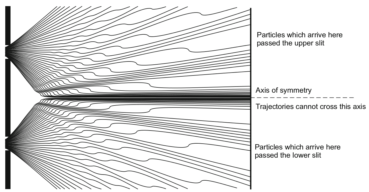
Figure 2: Possible trajectories for a particle in the famous double slit experiment Phi79 . After passage through the slits, the guiding wave $\psi$ of every particle forms a diffraction pattern according to Huygens’ principle. After the slit, this diffracted wave determines the possible trajectories of the particle.

In Bohmian mechanics the wave always goes through both slits and the particle goes through only one. But the particle is guided by the wave toward places where $|\psi|^{2}$ is large, and away from places where is small. As any wave would do, after passage through the slits, the guiding wave $\psi$ of every particle forms a diffraction pattern and so if a plate is in position the particle contributes a spot to the IP which is essentially the quantum equilibrium distribution on the plate at their point of arrival, this is clear enough, because that is what the quantum equilibrium hypothesis says. In no case the earlier motion, of either particle or wave is affected by the later insertion or non insertion of the plate (see Fig.2).

This result is clear, but the double slit experiment is often taken in textbooks as proof that one cannot have moving particles in quantum physics.

In general is not useful compute Bohmian trajectories in various quantum mechanical situations, what we learn in general from the trajectories is that, at each moment of time $t$, the particles have positions which are distributed according to the quantum equilibrium hypothesis. In Bohmian mechanics we can make more detailed predictions about the behaviour of individual elements in the ensemble. We cite 4 examples of predictions pertaining to individual particles in the double slit experiment DS09 :

1. The trajectories cannot cross the axis of symmetry.

2. The trajectories move mostly along the maxima (hyperbola) of $|\psi|^{2}$ and spend only short times in the valleys of $|\psi|^{2}(|\psi|^{2}\approx 0)$.

3. The trajectories cross the valleys since, right after the slits, the trajectories expand radially. This is turn happens because the guiding wave is a spherical wave close behind the slits, and while first feeding the nearest maxima, they must observe quantum equilibrium. Most trajectories will have to lie in the region of the main maximum (around the symmetry axis, which is the most clearly visible on the screen), i.e., trajectories must cross over from adjacent maxima to the main maximum.

4. The arrival spot on the screen is random, in particular the slit through which each particle goes is random. The randomness is due to the random initial position $Q_{0}$ of the particle with respect to the initial wave packet. By always preparing the same wave packet $\psi$, one prepares an ensemble of $|\psi|^{2}$ distributed positions.

We emphasize that these predictions concerning individual behaviour do not contradict the statistical ones of quantum mechanics. Their purpose is simply to contribute to the explanation of how the latter come about.

4.5 Delayed-choice experiments from the Bohmian perspective

“Is it not clear from the smallness of the scintillation on the screen that we have to do with a particle? And is it not clear, from the diffraction and interference patterns, that the motion of the particle is directed by a wave? De Broglie showed in detail how the motion of a particle, passing through just one of two holes in screen, could be influenced by waves propagating through both holes. And so influenced that the particle does not go where the waves cancel out, but is attracted to where they cooperate. This idea seems to me so natural and simple, to resolve the wave-particle dilemma in such a clear and ordinary way, that it is a great mystery to me that it was so generally ignored.” Bel87 Bell

The traditional demonstration that one cannot simultaneously observe the ‘path’ a particle takes through an interferometer and the IP it contributes to rests on an application of the Heisenberg relations. It has not been generally appreciated that the desired result may be arrived at without any direct invocation of Heisenberg’s relations, but follows from general properties of the many-body interaction between a coherent system and a detector. This seems to provide a deeper understanding of the problem in that applications of Heisenberg’s relations have tented to rely on arguments drawn from classical optics whose connection with the quantum formalism is not always clear. We shall see that even if the coherence of the interfering beams is not destroyed by the external path-measuring agency, interference will still not be observed in situations where we determine the ‘path’. Actually, the usual approach to this problem, however it proceeds, is deficient in one fundamental respect

It seeks to define the conditions under which one can or cannot have definite knowledge about the ‘path’ a quantum particle takes while working with the formalism of orthodox quantum mechanics within which such a notion is meaningless in all circumstances.

To discuss this problem consistently means admitting that $\psi$ provides an incomplete description of individual events and must be supplemented by the idea that in our world, electrons and other elementary particles have precise positions ${\bf Q}_{k}(t)\in\mbox{${\rm I\!R}$}^{3}$ at every time $t$ that move according to (4). That is, for a certain trajectory $t\mapsto Q(t)$ in configuration space, it claims that $Q(t)=({\bf Q_{1}}(t),\cdots,{\bf Q_{N}}(t))$ is the configuration of particle positions in our world at time $t$.

This, of course, is precisely what Bohmian mechanics provides and it is our purpose here to put on a secure conceptual footing the proof of the impossibility of simultaneous measurement of a particle position and an interference image (‘simultaneous’ means that in an individual case we obtain a particle position and contributes to an IP generated by the overlap of two coherent waves which is essentially the quantum equilibrium $|\psi|^{2}$ distribution). Notice that we don’t say measurement of the trajectory since as consequence of the uncertainty principle is impossible measure the trajectory of an individual particle takes, because any measurement of position irrevocably disturbs the momentum, and vice versa. Using weak measurements, however, it is possible to operationally define a set of trajectories for an ensemble of quantum particles KBRSMSS11 .

We also show that the trajectory assumption is not disproved by the traditional argument and on the contrary, it serves to justify the latter. Remember that we consider the wave function as nomological and is still relevant when we possess the particle position because particles move in a way that depends on the wave function. Notice that the notion of ‘wave-particle duality’ refers to ‘complementarity’ does not apply in our model.

Consider a beam of particles (normalized wave packet $\psi$) sent through on a beam splitter which produces two ensembles of independent subsystems (two packets $\psi_{1}$ and $\psi_{2}$) that propagate along the arms of an interferometer. A device designed to measure the position of the particle ($x$-system) is situated in the upper arm. The meter needle of this device has initial coordinate $y_{0}$ in a normalized packet $\phi_{y_{0}}$. It is assumed that $\psi_{1}\cap\psi_{2}=0$ in order that the observing apparatus interacts only with $\psi_{1}$.

According to orthodox quantum measurement theory, after a measurement, or preparation, has been performed on a quantum system, in this case the $x$-system, the wave function for the composite formed by system and apparatus is of the form DGN13

$$\sum\limits_{\alpha}\psi_{\alpha}\otimes\phi_{\alpha}$$ (10)

With the different $\phi_{\alpha}$ supported by the macroscopically distinct (sets of) configurations corresponding to the various possible outcomes of the measurement, e.g., given by apparatus pointer orientations. Of course, for Bohmian mechanics the terms of (10) are not all on the same footing: one of them, and only one, is selected, or more precisely supported, by the outcome, corresponding, say, to $\alpha_{0}$ which actually occurs. To emphasize this we may write (10) according to (9) in the form

$$\psi\otimes\phi+\Psi^{\perp}$$

Where $\psi=\psi_{\alpha_{0}}$, $\phi=\phi_{\alpha_{0}}$, and $\Psi^{\perp}=\sum\limits_{\alpha\not=\alpha_{0}}\psi_{\alpha}\otimes\phi_{\alpha}$. It follows that after the measurement the $x$-system has effective wave function $\psi_{\alpha_{0}}$. We can determine the position of the particle by performing a sharp position measurement. However, a position determination only requires a ‘weaker measurement’ which locates the particle in the region of space where $\psi_{1}$ is finite. Hence, we assume that the interaction with the observing device does not appreciably alter $\psi_{1}$.

The aim in this case is to maximize the perturbation of the $x$-system and minimize that between the initial and final states of the $y$-system (apparatus). We shall show that these are mutually incompatible requirements. At the exit to the beam splitter the total wave function is

$$\psi_{0}=[\psi_{1}+\psi_{2}]\phi_{y_{0}}$$

$$\rightarrow f+\psi_{2}\phi_{y_{0}}\$$

$$\rightarrow\psi=\psi_{1}\phi_{y}+\psi_{2}\phi_{y_{0}}$$

After the interaction, where $\phi_{y}$ is the final state of the meter and where, as we have said, $\psi_{1}$ is essentially unaltered. If $\psi_{1}$ and $\psi_{2}$ still do not overlap, the configuration space summands in will not overlap and the system point to which $x$-system belongs is in one of them. However, in order to say unambiguously which one from observation of the various possible outcomes of the measurement, we must require that $\phi_{y_{0}}$ and $\phi_{y}$ are disjoint $(\phi_{y_{0}}\cap\phi_{y}=0)$, that is the initial and final apparatus states must be orthogonal. The position of the particle is then determined by the distinguishable outcomes of the meter and we may infer the ‘path’ from how the coordinate $y$ changes

$$\begin{cases}x\in\psi_{1}\ \mbox{iff}\ y_{0}\rightarrow y\in\phi_{y}\\ x\in\psi_{2}\ \mbox{iff}\ y_{0}\rightarrow y\in\phi_{y_{0}}\end{cases}$$

But, under these circumstances, no interference will be observed when $\psi_{1}$ and $\psi_{2}$ subsequently overlap, whatever route the particle took

$$I={|\psi_{1}|}^{2}+{|\psi_{2}|}^{2}+[c\psi_{2}^{*}\psi_{1}+cc]$$ (11)

Where

$$c=\phi^{*}_{y_{0}}\phi_{y}$$ (12)

Clearly, if $c=0$ the interference terms vanish. We conclude that a determination of the position of a particle in an interferometer is incompatible with the observation of interference. The general principle at work that causes the pattern to be washed out is clear, the mere fact that there is an exchange of energy or momentum between the system and apparatus. The nub of the issue is that in order to perform its role and unambiguously reveal a change, the initial an final states of the observing device must be orthogonal. Between the extremes of $\phi_{y}=\phi_{y_{0}}$ (maximum contrast) and $\phi_{y_{0}}\cap\phi_{y}=0$ (no interference) there is a continuous range of diminutions in the contrast of the IP depending on the extend of the overlap of $\phi_{y_{0}}$ and $\phi_{y}$. Then is impossible obtain an exact position of the particle, except when $\phi_{y_{0}}\cap\phi_{y}=0$. Our argument against the possibility of a simultaneous observation of position and interference is evidently of a general character and not dependent on the nature of the interacting systems. Notice also that we arrive at this conclusion without invoking the ‘collapse of the wave function’ on ‘measurement’.

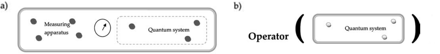
Figure 3: (a) A Bohmian measurement assumes that the quantum system and the measuring apparatus are explicitly simulated OM12 . (b) The orthodox measurement assumes that only the quantum system is explicitly simulated, but the measuring apparatus is substituted by an operator acting on the wave function of the system.

This is how collapse (or reduction) of the effective wave function to the one associated with the outcome $\alpha_{0}$ arises in Bohmian mechanics. While in orthodox quantum mechanics the ‘collapse’ is merely superimposed upon the unitary evolution without a precise specification of the circumstances under which it may legitimately be invoked, we have now, in Bohmian mechanics, that the evolution of the effective wave function is actually given by a stochastic process, which consistently embodies both unitarity and collapse clearly and unambiguously (see Fig.3). In particular, the effective wave function of a subsystem evolves according to Schrödinger’s equation when this system is suitably isolated. Otherwise it “pops in and out” of existence in a random fashion, in a way determined by the continuous (but still random) evolution of the conditional wave function $\psi_{t}$ DGN13 . Moreover, it is the critical dependence on the state of the environment and the initial conditions which is responsible for the random behavior of the (conditional or effective) wave function of the system.

Because in Bohmian mechanics the wave function is more than a mere repository of our current information about a system, and its law of motion induces that of the particle, it is a natural to expect that the insertion of a probe in the apparatus to check the above predictions will modify the wave in such a way that the particle trajectory suffers a disturbance. It has been proposed that such experiments allow one to glean varying degrees of ‘knowledge’ of the ‘particle and wave aspects of matter’. Is necessary clarify the significance has been attributed in the literature to the circumstances that the fringes may remain substantially visible when the ‘particle knowledge’ is relatively large. This is a simple consequence of the definition of the contrast of an interference pattern Hol93 .

Let $\psi=\psi_{B}+\psi_{B^{\prime}}$, where $\psi_{b},\psi_{B^{\prime}}$ are arbitrary waves of amplitude $R_{b},R_{B^{\prime}}$, and write $I=|\psi|^{2}$. Then the contrast, which has been presented as a measure of our ‘wave knowledge’, is defined by:

$$V=\frac{I_{max}-I_{min}}{I_{max}+I_{min}}=\frac{2R_{B}R_{B^{\prime}}}{R_{B}^{2}+R_{B^{\prime}}^{2}}$$ (13)

With $0\leq V\leq 1$. As the ratio $\frac{R_{B^{\prime}}}{R_{B}}$ decreases, $V$ decreases but at a slower rate. To bring out the implications of this define a ‘complementary’ quantity characterizing the ‘particle knowledge’

$$K=\frac{R_{B}^{2}-R_{B^{\prime}}^{2}}{R_{B}^{2}+R_{B^{\prime}}^{2}}$$ (14)

We have

$$K^{2}+V^{2}=1$$ (15)

The problem with this discussion is that for it to be meaningful we must give credence to the notion that a particle has a ‘path’ through the interferometer that we could have ‘knowledge’ of. This concept has been slipped in without an explicit recognition that it is an additional assumption. In this fact, only in Bohmian mechanics that the ‘which-path’ debate fully makes sense.

The mathematical discussion presented above does not require quantum mechanics at its heart. In particular, the derivation of (15) is essentially in terms of the diffraction and interference of waves valid for waves of any sort. In this connection one must remember that $V$ and $K$ defined above are primarily expressions reflecting properties of the interfering waves and their variation represents objective changes in the system (note that in general they are functions in space). As secondary properties is possible apply this result to the wave function of a quantum system to yield statistical information of it. In that case (15) is known as the Englert-Greenberger duality relation (1).

5 Afshar’s experiment again

The discussion around if the Afshar’s experiment violates (1) and so the ‘principle of complementarity’ is kind of silly. The ‘principle of complementarity’ is ill defined and this makes the critical analysis difficult. What we mean is this: wave and particle are words, they have of course through everyday language a clear connotation but since we are doing physics, these words have to be linked to physics, i.e., to a physical theory. Now in the Copenhagen interpretation, these linkage is not done via a theory but through experimental setups. Those experimental setups are supposed to ‘define’ what particle and what wave mean. That is of course delicate and obscure, and that is the problem with the ‘principle of complementarity’. Suppose you have an experiment which defines ‘particle’, for example because the experimental data are of position measurement and give the statistics as they are given by the amplitude square of the wave function. Then suppose you have another experiment which measures ‘wave’ (no such experiment exists!). Usually people think of IP in the modulus square of the wave function as such. Then combining such experiments one may derive some kind of relations like (1), but that relation holds then only for that kind of setup. It is a theoretical description of some kind of experimental setup. But through those words like ‘which-path’ and ‘interference’ such relations sound interesting. It is the way people talk without reference to a physical theory that things look interesting or mysterious.

Englert uses for the derivation of (1) in Eng96 an experimental setup analogous to the setup that we discussed in the section 4.5. We have shown in that section from the Bohmian perspective the explanation of why a determination of the position of a particle in an interferometer is incompatible with the observation of interference, i.e., that in an individual case if we obtain the particle position that particle can’t contributes to an IP generated by the overlap of two coherent waves.

The Afshar’s experiment setup is a very different kind of setup, in stage (iii) the contrast is inferred using (13), which is essentially measure the minimum intensity of the dark fringe $I_{min}\approx 0$ from comparative measurements of the total flux with and without the WG AFMK07 :

$$V=\frac{I_{max}-I_{min}}{I_{max}+I_{min}}=\frac{I_{max}}{I_{max}}=1$$

This process clearly doesn’t affect the quantum equilibrium distribution and allows to perform the ‘which-path’ measurement that as we explained in the last section is meaningless in terms of the orthodox interpretation of quantum theory. With this in mind now something is clear, The Afshar’s experiment correspond to a very different physical process for which (1) was not compute and therefore doesn’t apply.

The characterization of the ‘wave and particle aspects of matter’ in the orthodox interpretation does not exhaust all we can say about these concepts and does not reflect the meaning given to them in Bohmian mechanics. In particular the function $K$ in (1) and (14) has no connection with the Bohmian trajectories. The fact is that orthodox quantum mechanics not simply a theory of our knowledge of physical systems, a kind of generalization of classical statistical mechanics without the trajectories, and diffraction phenomena demonstrate this.

We hope that our analysis can contribute to clarify the confused debate originated by the orthodox analysis of the Afshar’s experiment. While this results may not appear as a big surprise the Afshar’s experiment is not trivial. We have shown with the previous discussion an example of the paradoxes that may arise if one attempts to artificially subdivide quantum phenomena and pretend to study it adopting an inconsistent model to describes what a quantum particle is and how it behave. To avoid the paradoxical conclusion of the orthodox interpretation of quantum theory that apparently flowing from the ‘delayed-choice’ class of experiments, i.e., that the decision on whether to insert the counters (and hence determine ‘which-path’) or to leave them out and let the electron contribute to the IP (the electron takes ‘both paths’) may be made after the electron has ‘passed’ the slit plane and so the that the earlier behaviour of the electron (passage through one or both slits) may be influenced by our later decision whether or not to insert the counters. It is proposed by Wheeler against this nonsense and in defence of a ‘consistent’ orthodox interpretation, that matter has disappeared!! and so to be is to be perceived!!, he himself seems to be very clear on this point. He says:

“After the quantum of energy has already gone through the doubly slit screen, a last-instant free choice on our part–we have found–gives at will a double-slit-interference record or a one-slit-beam count. Does this result mean that present choice influences past dynamics, in contravention of every formulation of causality? Or does it mean, calculate pedantically and don’t ask questions? Neither; the lesson presents itself rather as this, that the past has no existence except as it is recorded in the present. It has no sense to speak of what the quantum of electromagnetic energy was doing except as it is observed or calculable from what is observed.” Whe78

This conclusion is often cited as conflicting with the idea that there can be particles with trajectories(or more general as conflicting with the idea of the existence of an external real world out there and that it is the task of physics to find the basic constituents of this exterior real world and the laws that govern them). One sends a particle through a double slit (i.e., a wave packet $\psi$). Behind the slit at some distance is a photographic plate. When the particle arrives at the plate it leaves a black spot at its place of arrival. Nothing yet speaks against the idea that the particle moves on a trajectory. But now repeat the experiment. The next particle marks a different spot of the photographic plate. Repeating this a great many times the spots begin to show a pattern. They trace out the points of constructive interference of the wave packet $\psi$ which, when passing the two slits, shows the typical Huygens interference of two spherical waves emerging from each slit. Suppose the wave packet reaches the photographic plate after a time $T$(this time is defined in terms of the motion of the centre of a wave packet). Then the spots show the $|\psi(T)|^{2}$ distribution, in the sense that this is their empirical distribution. Analyzing this using Bohmian mechanics mechanics, i.e., analyzing Schrödinger’s equation and the guiding equation, one immediately understands why the experiment produces the result it does. It is clear that in each run the particle goes either through the upper or through the lower slit. The wave function goes through both slits and forms after the slits a wave function with an IP. Finally the repetition of the experiment produces an ensemble which checks Born’s statistical law for that wave function. That is the straightforward physical explanation. So where is the argument which reveals a conflict with the notion of particle trajectories? Here it is:

From equations (11) and (12) we can observe that in general:

$$I={|\psi_{1}|}^{2}+{|\psi_{2}|}^{2}+[c\psi_{2}^{*}\psi_{1}+cc]\not={|\psi_{1}|}^{2}+{|\psi_{2}|}^{2}$$ (16)

Wheeler arrives at his conclusion invoking (16), one of the apparent non-localities of orthodox quantum mechanics, i.e., the instantaneous, over all space, ‘collapse of the wave function’ on ‘measurement’ Bel87 .

The Afshar’s experiment although not violate (1), show a very important result, Afshar observes that the amount of light intercepted by the WG is very small, is maximally $1\%$ AFMK07 . This is a clear experimental proof of the prediction 2 that Bohmian mechanics makes concerning to the double-slit experiment that we reference in the section 4.4 and more important, this mean that (16), i.e., the mathematical expression of ‘decoherence’, can’t give a complete account of the quantum process and so is necessary a theory that provide us with a coherent story about the complete quantum process itself. This, of course, is precisely what Bohmian mechanics provides, interpreting the problem simply as evidence of the incompleteness of quantum theory. The passage of the corpuscle through one slit and the wave through both forms a well-defined time-dependent physical process in itself. What happens subsequently has no bearing on it at all. If both paths through the interferometer are open the particle will respond to the overlapping waves. The detecting plate reveals that this has happened, but does not influence it. If instead the counters are inserted prior to the overlap of the waves the evolved wave is different and in detecting the particle the counters again simply reveal this. According to Bohmian mechanics, The present merely reveals the past and has no influence upon it. In this regard at least there is no need to revise our customary conceptions of cause and effect, nothing simply surges up out of nothing without having antecedents that existed before. Likewise, nothing ever disappears without a trace, in the sense that it gives rise to absolutely nothing existing at later times. This principle is not yet a statement of the existence of causality in nature. Indeed, it is even more fundamental than is causality, for it is at the foundation of the possibility of our understanding nature in a rational way Boh71 .

6 Bohmian trajectories as the foundation of quantum mechanics

The core of orthodox quantum mechanics is that physics is about measurement and observation, and not about an objective reality, about what seems, i.e., ‘observation’ or ‘sensations’ or ‘information’ or ‘data’ and not about what is about the things-in-themselves!.

We think that a fundamental physical theory should not be formulated in terms of concepts like ‘observer’ or ‘experiment,’ as these concepts are very vague and certainly do not seem fundamental. Is a cat an observer? A computer? Were there any experiments before life existed on Earth? If consciousness causes collapse and consciousness is a product of the brain What about the collapse of the brain? Does man think with the help of the brain?

In this work we have studied only a simple example of the crisis in quantum physics, but the essence of the crisis consists in the rejection of an objective reality existing outside the mind. ‘Matter has disappeared’ one may thus express the fundamental and characteristic difficulty in relation to many of the particular questions, which has created this crisis. The idea that now dominates the minds of physicists is that laws of motion can be treated mathematically and therefore that mathematics can to overlook matter. ‘Matter disappears,’ only equations remain.

In this new stage of development and apparently in a new manner, we get the old Kantian idea: reason prescribes laws to nature. This, of course, is a ridiculous dream. ‘Matter is disappearing’ means that the limit within which we have hitherto known matter is vanishing and that our knowledge is penetrating deeper; properties of matter are likewise disappearing which formerly seemed absolute, immutable, and primary and which are now revealed to be relative and characteristic only of certain states of matter.

The sole property of matter that necessarily must be recognized by physics to advance is the property of being an objective reality, of existing outside our mind.

In a nutshell, the quantum philosophy of today is the same ‘philosophical idealism’ of yesterday, this means that one school of scientists in one branch of natural science has slid into an absurd philosophy. The abandonment of these ideas is being made, and will be made, by quantum physics; but it is making not directly, but by zigzags, not consciously but instinctively, not clearly perceiving its ‘final goal,’ but drawing closer to it gropingly, hesitatingly, and sometimes even with its back turned to it. Quantum physics is in travail; it is giving birth to future. The process of child-birth is painful. And in addition to a living healthy being, there are bound to be produced certain dead products, refuse fit only for the garbage-heap. And the entire school of positivism and empirio-critical philosophy, together with empirio-symbolism, empirio-monism, and so on, and so forth, must be regarded as such refuse!

Bohmian trajectories have been used for various purposes, including the numerical simulation of the time-dependent Schrodinger equation and the visualization of time-dependent wave functions WT05 . But we have showed in a simple example their real purpose they were invented for: to serve as the foundation of quantum mechanics, i.e., to explain quantum mechanics in terms of a materialistic theory, providing the foundation for the claim that a fundamental physics focused on an objective reality existing outside the mind is possible, providing a theory free of paradoxes and allows an understanding that is as clear as that of classical mechanics, this means, while expressed in precise mathematical terms is also clear as physics.

One of the most absurdity objections to Bohmian mechanics is that is more complicated than orthodox quantum theory, since it involves an extra equation and is not ‘economical’. One has only to put this objection in order to see the absurdity, the subjectivism of applying the category of ‘the economy of thought’ here. Human thought is ‘economical’ only when it correctly reflects objective truth, and the criterion of this correctness is practice, experiment and industry BASMO14 , all mysteries which lead a theory to mysticism find their rational solution in human practice and in the comprehension of this practice.

Bohmian mechanics emerges as a precise and coherent quantum theory providing a microscopic foundation for the quantum formalism. To sum up, it seems fair to say that Bohmian mechanics is not an interpretation of anything it is a complete theory where nothing is left open, and above all, it does not need an interpretation. It is a theory of nature, and it has a precise link to quantum mechanics. At the end of the day, the fundamental reasons for the dismissal seems to be this: Bohmian mechanics is against the spirit of quantum mechanics. That is, an objective physical description, a return to determinism, a return to physical clarity clash with the tenets of ‘philosophical idealism’.

7 Towards a nonlinear quantum physics

7.1 The classical limit in Bohmian mechanics

As could be seen Bohmian mechanics provides a precise and coherent quantum theory with a microscopic foundation for the quantum formalism, giving a rigorous mathematical description together with a clear and unambiguous picture of the motion of quantum objects, in the non-relativistic regime.

Newtonian mechanics smoothly arises from special relativity as the speed of the system becomes smaller and smaller than the speed of light. This is possible because both theories are built upon the same conception of systems as localized (point-like) objects in space and time.

Similarly in quantum mechanics, according to standard textbook the criteria for the classical limit, it is often considered when $\hbar\to 0$ (or equivalently $\hbar\ll S_{cl}$ , where $S_{cl}$ denotes a related classical action). Therefore, in Bohmian mechanics everything should be very simple: the condition $\hbar\to 0$ should lead to classical mechanics. Bohmian mechanics has a very appealing feature regarding the quantum to classical transition: the quantum potential. This additional term to the Hamilton-Jacobi equation contains information about the topological curvature of the wave function in the configuration space and is proportional to $\hbar^{2}/m$:

$$m\frac{d^{2}\textbf{X}}{dt^{2}}=\textbf{F}+\textbf{F}_{Q}$$

$$m\frac{d^{2}\textbf{X}}{dt^{2}}\simeq\textbf{F}$$

Where $\textbf{F}=-\mbox{\boldmath$\nabla$\unboldmath}V(\textbf{X})$ and $\textbf{F}_{Q}=-\mbox{\boldmath$\nabla$\unboldmath}V_{Q}(\textbf{X})$ are respectively the classical force and the “quantum” force of a particle with trajectory $\textbf{X}=\textbf{X}(t)$.

This is the traditional classical limit. Now, $\hbar$ is just a constant and therefore is also possible think the classical limit in a more physical way, in terms of larger and larger masses.

Now, what happpend in this case? The quantum potential should also vanish and therefore the classical Hamilton-Jacobi equation should start ruling the system dynamics. What we observe as $m$ increases is that trajectories start mimicking the behavior of classical trajectories. One could be tempted to think that we are actually observing the emergence of classical trajectories. However, because of the intricate interference structure of the wave function, the quantum potential also exhibits a rather complex topology, such that the factor depending on the curvature of the wave function does not vanish. Consequently, one of the distinctive traits of Bohmian mechanics, the noncrossing rule, still remains valid.

The key ingredient in the analysis of the emergence of the classical world in Bohmian mechanics is then the following: If one observes the dynamics of the full-dimensional system (system of interest plus environment), the corresponding Bohmian trajectories satisfy the usual noncrossing rule. Now, these trajectories contain information about both the system and the environment.

In order to examine the system dynamics, one has to select only the respective components of those full-dimensional trajectories. This is equivalent to observing the dynamics in a subspace, namely the system subspace. It is in this subspace where the system trajectories display crossings, just because they are not (many-particle) Bohmian trajectories in the high-dimensional space, but trajectories onto a particular subspace, actually this leads us immediately to the notion of conditional wave function and his possible use to establish a bridge between these various subspaces. Here the role of the environment consists of relaxing the system noncrossing property by allowing its (reduced) trajectories to reach regions of the configuration subspace which are unaccessible when the system is isolated. This thus explains the phenomenon of decoherence.

In order to discuss the practical utility of these conditional wave functions, we need to explore the possibility of defining them independently of the big wave function, ie, find an equation to compute and analyse the dynamical evolution of a quantum (sub)system exclusively in terms of these single-particle (conditional) wave functions, instead of (as we did in their presentation) first solving the many-body Schrödinger’s equation for $\Psi$ and only examining the conditional wave functions $\psi$ after.

However, contrarily to the Schrödinger’s equation the new equation can be nonlinear. In other words, there is no guarantee that the superposition principle satisfied by the big wave function (in the big configuration space) is also applicable to the little (conditional) wave function when dealing with quantum subsystems.

This analysis is interesting in the context of collapse models. In Toros16 it is shown that the dynamics of the conditional wave function obeys to a collapse type of equation which, under reasonable assumptions, is that of the GRW model. In addition, for the center of mass the conditional wave function of a compositive system, an amplification mechanism is present, like in the GRW model.

7.2 Collapse models and the emergence of classicality

The Ghirardi-Rimini-Weber (GRW) model of spontaneous wave function collapse as well as Bohmian mechanics are the basis of the research program outlined by John S. Bell in 1987, the GRW model was proposed as a solution of the measurement problem of quantum mechanics and involves a stochastic and nonlinear modification of the Schrödinger’s equation. It deviates very little from the Schrödinger’s equation for microscopic systems but efficiently suppresses, for macroscopic systems, superpositions of macroscopically different states and as suggested by Bell, the primitive ontology, or local beables, of the model are the discrete set of space-time points, at which the collapses are centered. This set is random with distribution determined by the initial wavefunction.

The aim of the dynamical reduction program is then modify the Schrödinger’s equation, by introducing new terms having the following properties:

• They must be non-linear, as one wants to break the superposition principle at the macroscopic level and assure the localization of the wave function of macro-objects.

• They must be stochastic because, when describing measurent-like situations, is neccesary explain why the outcomes occur ramdonly; more than this, is neccesary explain why are they distributed according to the Born probability rule

• The must be an amplification mechanism according to which the new terms have negligible effects on the dynamics of microscopic systems, but at the same time, their effects becomes very strong for large many-particle systems such as macroscopic objects, in order to recover their classical-like behavior.

We limit the presentation to the GRW model, is neccesary clarify this because there are other models of spontaneous wave function collapse (collapse models). In particular, we present the formulation of the GRW model due to J.S. Bell.

Let us consider a system of $N$ particles which for simplicity we take to be scalar. This system in the GRW model is described by a wave function $\psi(x_{1},x_{2},\dots x_{N})$ belonging to the Hilbert space $\mathit{L}^{2}(\Re^{3N})$ and at random times, each particle experiences a sudden jump of the form:

$$\psi_{t}(x_{1},x_{2},\dots x_{N})\to\frac{\hat{L}_{n}(x)\psi_{t}(x_{1},x_{2},...x_{N})}{\|\hat{L}_{n}(x)\psi_{t}(x_{1},x_{2},...x_{N})\|}$$

Where $\psi_{t}(x_{1},x_{2},\dots x_{N})$ is the state vector of the whole system at time $t$, immediately prior to the jump process. $\hat{L}_{n}(x)$ is a linear operator called the reduction operator (the operator on whose eigenfunctions one wants to reduce the statevector, as a consequence of the collapse mechanism) which is conventionally chosen equal to:

$$\hat{L}_{n}(x)=\sqrt[4]{\left(\frac{\alpha}{\pi}\right)^{3}}e^{-\frac{\alpha}{2}(\hat{q}_{n}-x)^{2}}$$ (17)

Where $\alpha$ is a new parameter of the model with sets that the width of the localization process, and $\hat{q}_{n}$ is the possition operator associated to the $n-$th particle; the random variable $x$ correspond to the place where the jumps occurs. Between two consecutive jumps, the state vector evolves according to the Schrödinger’s equation.

The probability density of a jump taking place at the possition $x$ for the $n-$th particle is given by:

$$p_{n}(x)\equiv\|\hat{L}_{n}(x)\psi_{t}(x_{1},x_{2},\dots x_{N})\|^{2}$$

And the probability densities for the different particles are independent. Finally it is assumed that the jumps are distributed in time like a Poissonian process with the frecuency $\lambda$, which is the second new parameter of the model.

The standard numerical values for $\lambda$ and $\alpha$ are:

$$\lambda\simeq 10^{-16}s^{-1},\qquad\alpha\simeq 10^{10}cm^{-2}$$

Then, the first parameter(the collapse strength) sets the strength of the collapse mechanics for one particle, and through the amplification mechanism also for a macroscopic system. And $r_{C}=1/\sqrt{\alpha}$ (the spatial correlation function of the noise, which determines the width of the localization gaussian in (17)) tell which kind of superpositions are effectively supressed, and which not. In the case of a compositive system, an object, in a superposition of two different states, distant relative to each other more than $r_{C}$. The collapse mechanism becomes difficult to ulfold analytically, due to the complexity of the dynamics for the system. Nevertheless is possible work out an easy approximative rule to estimate the effect. The center of mass of the system collapses with a rate

$$\Gamma=\lambda n^{2}N$$

where $\lambda$ is the collapse rate of a single constituent (a nucleon), $n$ is the number of constituents contained in a volume of radius $r_{C}$ (therefore it is a measure of the density of the system) and $N$ counts how many such volumes can be accommodated in the system (therefore being a measure of the total volume of the system).

Finally, let the $m_{n}$ be the mass associated to the $n-$th “particle” of the system; then the function:

$$\rho_{t}^{(n)}(X_{n})\equiv m_{n}\int d^{3}x_{1}\dots d^{3}x_{n-1}d^{2}x_{n+1}\dots d^{3}x_{N}\>|\psi_{t}(x_{1},x_{2},\dots x_{N})|^{2}$$

represents the density of mass of that “particle” in space, at time t.

With the help of these axioms the GRW model tries to provide a unified description of all physical phenomena, at least at the non-relativistic level, and a consistent solution to the emergence of classicality. This because the collapse rate of a composite system scales with its size: the bigger the system, the faster the collapse. This is precisely the reason why collapse models can accommodate, within a single dynamical equation, both the quantum properties of microscopic systems (few constituents) and the classical properties of macroscopic objects (many constituents). In doing this, collapse models explain the quantum-to-classical transition, how the probabilistic and wavy nature of atoms and molecules gives rise to the world of classical physics as we experience it, when they glue together to form larger and larger objects, ie, the wave functions of macro-objets are almost allways very well localized in space, so well localized that their centers of mass behave, for all practical purposes, like point-particles moving according to Newton’s laws. In the other hand at the microscopic level, quantum system behaves almost exactly as predicted by orthodox quantum mechanics, and in measurement-like situation, e.g. of the Von neumann type reproduces as a consequence of the modified dynamics the Born probability rule and the collapse of the wave function.

The GRW then leads to a collapse process that is adequate to explain all present experimental results but, inevitably, although it solves some problems it produces others. In particular. It has been criticized because in the same way of all most important dynamical reduction models, which aim at localizing wavefunction in space, exhibit the typical feature of violating the energy conservation for isolated systems. In fact if one choose $\hat{L}$ to be the position operator $\hat{q}$ or a function of it, like (17) (the reason to use the position operator is that is the most natural candidate for localizing wavefunctions in space), then it can be shown that the amplification mechanism induces larger and larger fluctuations in the momentum space as one can roughly infer using the uncertainty principle: The smaller the uncertainty in position the bigger uncertainty in momentum. Such fluctuations, in turn, determine the growth of the energy of the system, which eventually diverges for large times. Then, apparenly, the energy nonconservation appears to be an intrinsic property of collapse models since the stochastic process driving the reduction mechanism seems to be directly responsible for such a violation.

Now, it is neccesary to stress some points about the world-view provides by the GRW model. According to the ontological interpretation of this theory, there are no particles at all in the theory! There are only distributions of masses which, at the microscopic level, are in general quite spread out. An electron, for example, is not a point following a trajectory as in Bohmian mechanics  but a wavy system diffusing in space. When in the double-slit experiment, or more specific in our case, in the Afshar’s experiment , it goes through the both of them, as a classical water-wave would do. The peculiarity of the electron, which qualifies it as a quantum system, is that when we try to localize it in space by letting it interacting with a measuring devise, e.g. a photographic plate, then, according to the localization process and because the interaction with the plate, its wave function very rapidly shrinks in space till is gets localized to a spot, the spot where the plate is impressed and which represents the outcome of the measurement. The big difference between GRW and orthodox quantum mechanics is that such a behaviour is not accounted by a crude “instantaneous collapse” prescription, with has no explanation within the theory, conversely it is a direct consequence of the universal dynamics of the GRW model, also in it framework even though the GRW model contains no particles at all, is usually referred to microsystems as “particles”, just for a matter of convenience, this because also macroscopic objects in this model are waves, their centers of mass are not mathematical points, rather they are represented by some function defined throughout space, but with the property of be always almost perfectly located in space, which means that the wave function associated to their centers of mass are appreciably different from zero only within a very tiny region of space, so tiny that can be consider point-like for all practical purposes such dynamics is governed by Newton’s laws.

In Toros16 it is shown how Bohmian trajectories become classical when particles glue together to form macroscopic objects, which unavoidably interact with the surrounding environment, the dynamics of this process obeys in a first approximation a collapse process similar to the postulated in the GRW model. This might open the way to finding an underlying theory. These two theories are always presented as dichotomical, but as shown in Allori02 they have much more in common that one would expect at first sight. The differences are less profound than the similarities and then using the common structure of them would be possible formulate a new theory with benefits from Bohmian mechanics and the GRW model and (collapse models in general).

7.3 The non-local ontology of the Ghirardi-Rimini-Weber model

“Either the wave function as given by the Schrödinger’s equation, is not everything, or it is not right.” Bell

How we as shown in this work Bohmian trajectories serve to explain quantum mechanics in terms of a materialistic theory, providing the foundation for the claim that a fundamental physics focused on an objective reality outside the mind is possible. But this is not the case of the GRW model where only the wave function is regarded as existing, the basic problem of this theory is that never talks about matter, and then would not form an adequate description of the world. Strictly speaking, in a world governed by such a theory there exist no matter neither a clear link between the objective reality and the mathematical variables of the theory.

Even worse, if we use the GRW model to deal with the Afshar’s experiment paradox we get the same problem of orthodox quantum mechanics. In general the problem that it remains to be clarified is in what the way the wave functions $\psi_{\Sigma}\wedge\psi_{\Sigma^{\prime}}$ associated with different regions $\Sigma\wedge\Sigma^{\prime}$ of the space have to be compatible to be regarded as describing a consistent reality. In the case $\Sigma\wedge\Sigma^{\prime}$ have a large portion in common like in the Afshar’s experiment, is necessary that $\psi_{\Sigma}\wedge\psi_{\Sigma^{\prime}}$ describe the same reality on $\Sigma\cap\Sigma^{\prime}$. This is one of the problems in the GRW model and we need define clearly what that reality is and how the wave function influences that reality.

Assuming that $\psi_{\Sigma}\wedge\psi_{\Sigma^{\prime}}$, are the wave functions associated to different regions of space, any of them, suppose wave function $\psi_{\Sigma}$ can be constructed by superposing, in the same region of space, waves of slightly different wavelengths, but with phases and amplitudes chosen to make the superposition constructive in the desired region and destructive outside it. Mathematically, we can carry out this superposition by means of non-local Fourier analysis. For simplicity, we are going to consider a one-dimensional wave packet. Then, we construct the packet $\psi_{\Sigma}(x,t)$ by superposing plane waves(propagating along the $x$-axis) of different frecuencies (or wavelengths):

$$\psi_{\Sigma}(x,t)=\frac{1}{\sqrt{2\pi}}\int_{-\infty}^{+\infty}\phi(k)e^{i(kx-\omega t)}dk$$ (18)

where $\phi(k)$ is the amplitude of the wave packet. The packet is intended to describe a particle confined to a one-dimensional region, in this case a particle moving along the $x$-axis. We want to look at form of the packet at a given time. Choosing this time to be $t=0$ and abbreviating $\psi_{\Sigma}(x,0)$ by $\psi_{\Sigma_{0}}$, we can reduce (18) to:

$$\psi_{\Sigma_{0}}(x)=\frac{1}{\sqrt{2\pi}}\int_{-\infty}^{+\infty}\phi(k)e^{ikx}dk$$ (19)

and

$$\phi(k)=\frac{1}{\sqrt{2\pi}}\int_{-\infty}^{+\infty}\psi_{\Sigma_{0}}(x)e^{-ikx}dk$$ (20)

where $\phi_{k}$ is the Fourier transform of $\psi_{\Sigma_{0}}(x)$, and where

$$e^{ikx}=cos(kx)+isen(kx)$$ (21)

is the kernel of the transformation.

We refer to (19) as the synthesis equation and to (20) as the analysis equation for $\psi_{\Sigma_{0}}$. Then, is expected that the packet whose form is determined in this way by the $x$-dependence of $\psi_{\Sigma_{0}}$, does indeed have the required property of localization: peaks at $x=0$ and vanishes far away from $x=0$. The idea is that when $x\to 0$ then $e^{ikx}\to 1$; because the waves of different frequencies interfere constructively, and far away form $x=0$ (i.e., $\|x\|\gg 0$) the phase (21) goes through many periods leading to violent oscillations, thereby yielding destructive interference.

However, what we actually are doing here is taking the function that represents the information available on the physical situation, the wave function. The next step is to make the analysis using (20), that is, the decomposition in terms of the kernel (21) (i.e., the trigonometric functions sine and cosine that are defined from minus infinity $(-\infty)$ to infinity $(\infty)$ both in space and time) which amounts to find the coefficients for the sines and cosines or, in the case of a non-periodic function, the coefficient function $\phi_{k}$. After that, once these coefficients are known, one normally makes the synthesis of the initial function using (19).

Thus, when we sum a certain number of these waves to synthesise $\psi_{\Sigma}$ a problem arise. The wave function $\psi_{\Sigma}$ that according to the GRW model contains all the information of the system and is used to obtain the the density of mass in space is being synthesized with Fourier analysis and this analysis is non-local!, i.e., it kernel, it’s building blocks, are harmonic plane waves, and these harmonic plane waves are no more than sine and cosine functions, which are defined in whole space and in hole time. Then, at the microscopic level, the ‘particles’ according to the GRW model are in general quite spread out in a wavy system diffusing in space.

This is a serious problem, because within the GRW model with non-local Fourier analysis, all the ‘particles’ of the universe compose an infinite sea of density of mass, with only a potential existence that the collapse process materializes at a given position, and in this sense the GRW model fall in the same idealistic approach that orthodox quantum mechanics.

7.4 Perspectives: A theory of exclusively Local Beables

Using non-local Fourier analysis, as seen before, we were able to obtain the density of mass in space in the GRW model. However, this analysis is a non-local one, that is, it core are unlimited waves, either in space and time. Then, the non-local ontology of the GRW model comes from the way we mathematically represent the wave function.

We now propose a second possibility, This possibility is use Wavelet analysis. Wavelets were invented to overcome the shortcomings of Fourier analysis. With wavelets we can synthesize the wave function without gathering information contained in all space and time. Both analysis allows us to reconstruct the wave function. However, while Fourier analysis uses mathematical entities existing in whole space and whole time, Wavelet analysis use mathematical entities existing only locally.

For many decades scientist have wanted more appropriate functions than the sines and cosines, which are the basis of local Fourier analysis. These functions are non-local, they therefore do a very poor job in approximating sharp spikes. But with wavelet analysis, we can use approximating functions that are contained neatly in finite domains.

In 1975 Bell introduced the term beable to name whatever is posited, by a candidate theory, as corresponding directly to something that is physically real, i.e., independent of any observation. He then divides beables into two categories, local and non-local. In this sense, a theory as proposed above can be consider a theory of exclusive local beables. And it would provide also a concrete example of an empirical viable quantum theory in whose formulation the wave function on configuration space does not appear, i.e., it is a theory according to which nothing corresponding to the configuration space wave function need actually exist.

The idea with this is it might be possible to construct a plausible, empirically, viable theory of this kind, and to recommend this as an interesting and perhaps-fruitful program for future research. The theory of exclusive local beables put forward here is only an intended of toy model, to illustrate in principle that this kind of theory can, after all, be constructed. The challenge is then, for a system of $N$ particles moving in three spacial dimension, the theoretical description would be of $N$ wave functions. Now, there are some things we have to consider:

• The Schrödinger’s equation for an $N$-particle system is not a set of N (interacting) waves, each propagating in 3-space. It is a single wave propagating in $3N$-dimensional configuration space for the system.

• Schrödinger wave function for such an $N$-particle system living in the configuration space is by this characteristic a non-local agent, and any theory which aims to a correct description of nature must be non-local.

Fractal geometry is based on the idea of self-similar forms. To be self similar, a shape must be able to be divided into parts that are smaller copies which are more or less similar to the whole. Because of the smaller similar divisions of fractals, they appear similar at all magnifications. In this sense, non-locality could be recover in this model conserving the individuality of the beables through the use of multiresolution-based or fractal wavelets (Multi-resolution analysis (MRA)). A local beable of this nature is not a particle lying in space-time but, conversely, all the space-time is included in each beable.

In Bohmian mechanics the quantum potential leads to the notion of an “unbroken wholeness” and is the responsible for the non-local causality. On the other hand scale relativity with Hausdorff dimension $2$ is intimately related to the Schrödinger’s equation and quantum mechanics. If Einstein showed that space-time was curved, scale relativity shows that it is not only curved, but also fractal, i.e., that a space which is continuous and non-differentiable is necessarily fractal. It means that such a space depends on scale.

Importantly, scale relativity does not merely describe fractal objects in a given space. Instead, it is space itself which is fractal. To understand what a fractal space means requires to study not just fractal curves, but also fractal surfaces, fractal volumes, etc.

Mathematically, a fractal space-time is defined as a nondifferentiable generalization of Riemannian geometry. Such a fractal space-time geometry is the natural choice to develop this new principle of relativity, in the same way that curved geometries were needed to develop Einstein’s theory of general relativity.

Scale relativity predicts the existence of trajectories varying according to scale transformations. Those trajectories are not rectifiable, i.e., they are fractal. The apparently disordered motions of particles at the quantum scale are described in terms of motions following fractal geodesics.

As has been shown in Carroll12 , a recent paper of Kobelev describes a Leibniz type of fractional derivative and one can relate fractional calculus with fractal structures, then is shown that if is possible write a meaningful Schrödinger’s equation with Kobolev derivatives ($\alpha$-derivatives) then there will be a corresponding fractional quantum potential.

MRA could be a useful method for the construction of the neccesary nonlinear bases, since the linear harmonic analysis is inadequate for describing nonlinear systems. The wavelets in MRA are functions that have a space dependent scale which renders them an invaluable tool for analyzing multi-scale phenomena.

8 Conclusion

The aim of this thesis was use the Afshar’s experiment ‘paradox’ to try to answer the question, with what does the quantum mechanics actually deal ?. The answer given by Bohr (and within the framework of the usual interpretation the only possible consistent answer) is that it deals not with the properties of the objective reality as such but, rather, with nothing more than the relationships among the observable large-scale phenomena. The general point of view of Bohr has been given its most consistent and systematic expression, in terms of the ‘principle of complementarity’. The ‘principle of complementarity’ states that we are restricted to complementary pairs of inherently imprecisely defined concepts, such as position and momentum, wave and particle, etc. The maximum degree of precision of either member of such a pair is reciprocally related to that of the opposite member. This assumption leads to the conclusion that the basic properties of matter can never be understood rationally, e.g., an atom has no properties at all when it is not observed. Indeed, one may say that its only mode of being is to be observed; for the notion of an atom existing with uniquely definable properties of its own even when it is not interacting with a piece of observing apparatus, is meaningless within the framework of this point of view. We have shown however through the analysis of the Afshar’s experiment ‘paradox’ an example of why this response is unsatisfactory and leads to the current crisis in quantum physics, we have shown that the origin of this crisis consists in the rejection of an objective reality existing outside the mind, i.e., by try justify the tenets of quantum philosophy, namely ‘philosophical idealism’, through quantum physics, limiting the possible develop of quantum physics with the limits implicit in the ‘principle of complementarity’. We have shown that other answer to the question is possible using Bohmian mechanics. What does Bohmian mechanics contribute here? In a word, everything! Bohmian mechanics is a beautiful example of a theory that is satisfactory as a fundamental physical theory, a fundamental physical theory very different from classical mechanics, but we that it be as clear as classical mechanics. Bohmian mechanics is a counterexample to all claims that a rational account of quantum phenomena is impossible. It is also a counterexample to the claim that quantum mechanics proves that nature is intrinsically random that there is no way that determinism can ever be reinstated in the fundamental description of nature. This work is a simple example of why physics must be about the objective reality and need recognizes instead that a quantum theory must describe such a reality.

References

- (1) Afshar, S., Flores, E., McDonald, K., and Knoesel, E. Paradox in wave-particle duality. Foundations of Physics 37, 2 (2007), 295–305.
- (2) Afshar, S. S. Violation of the principle of complementarity, and its implications. In Optics & Photonics 2005 (Aug. 2005), C. Roychoudhuri and K. Creath, Eds., International Society for Optics and Photonics, pp. 229–244.
- (3) Aurélien Drezet. Complementarity and Afshar’s experiment.
- (4) Aurélien Drezet. Wave Particle Duality and the Afshar Experiment.
- (5) Bell, J. Against ”measurement”. 17–31.
- (6) Bell, J. S. Speakable and unspeakable in quantum mechanics. Collected papers on quantum philosophy. Cambridge University Press, 1988.
- (7) Benseny, A., Albareda, G., Sanz, . S., Mompart, J., and Oriols, X. Applied bohmian mechanics. The European Physical Journal D 68, 10 (2014).
- (8) Bohm, D. A suggested interpretation of the quantum theory in terms of ”Hidden” variables. I. Physical Review 85, 2 (Jan. 1952), 166–179.
- (9) Bohm, D. A suggested interpretation of the quantum theory in terms of ”Hidden” variables. II. Physical Review 85, 2 (Jan. 1952), 180–193.
- (10) Bohm, D. Causality and Chance in Modern Physics. Pennsylvania paperbacks. University of Pennsylvania Press, Incorporated, 1971.
- (11) Bohr, N. The quantum postulate and the recent development of atomic theory. Nature 121, 3050 (Apr. 1928), 580–590.
- (12) Carroll R. On a Fractional Quantum Potential. Progress in Physics (2012).
- (13) Daniel Reitzner. Comment on Afshar’s expriments.
- (14) Detlef Dürr, S. T. Bohmian Mechanics: The Physics and Mathematics of Quantum Theory, 1 ed. Fundamental Theories of Physics. Springer Berlin Heidelberg, 2009.
- (15) Detlef D rr, Sheldon Goldstein, N. Z. Quantum Physics Without Quantum Philosophy. Springer, 2013.
- (16) Englert, B.-G. Fringe visibility and which-way information: An inequality. Phys. Rev. Lett. 77, 11 (Sept. 1996), 2154–2157.
- (17) Flores, E., and Knoesel, E. Why kastner analysis does not apply to a modified afshar experiment, 2007.
- (18) Flores, E. V. Reply to Comments of Steuernagel on the Afshar’s Experiment. Foundations of Physics 38, 8 (2008), 778–781.
- (19) Holland, P. R. Quantum Theory of Motion, The: An account of the De Broglie-Bohm causal interpretation of quantum mechanics, 1 ed. Cambridge University Press, 1993.
- (20) Jacques, V., Lai, N. D., Dréau, A., Zheng, D., Chauvat, D., Treussart, F., Grangier, P., and Roch, J.-F. Illustration of quantum complementarity using single photons interfering on a grating. New Journal of Physics 10, 12 (Dec. 2008), 123009.
- (21) Kastner, R. Why the Afshar experiment does not refute complementarity. Studies in History and Philosophy of Science Part B: Studies in History and Philosophy of Modern Physics 36, 4 (Dec. 2005), 649–658.
- (22) Kastner, R. E. On visibility in the Afshar two-slit experiment. Foundations of Physics 39, 10 (Aug. 2009), 1139–1144.
- (23) Kocsis, S., Braverman, B., Ravets, S., Stevens, M., Mirin, R., Shalm, L., and Steinberg, A. Observing the average trajectories of single photons in a two-slit interferometer. SCIENCE 332, 6034 (3 July 2011), 1170 – 1173.
- (24) Mompart, X. O. J. Applied Bohmian Mechanics: From Nanoscale Systems to Cosmology. Pan Stanford Publishing, 2012.
- (25) Philippidis, C., Dewdney, C., and Hiley, B. Quantum interference and the quantum potential. Il Nuovo Cimento B (1971-1996) 52, 1 (1979), 15–28.
- (26) Qureshi, T. Comment on ”On Visibility in the Afshar Two-Slit Experiment”.
- (27) Qureshi, T. Modified Two-Slit Experiments and Complementarity. Journal of Quantum Information Science 02, 02 (June 2012), 34–39.
- (28) Robert E. Wyatt, C. J. T. Quantum Dynamics with Trajectories: Introduction to Quantum Hydrodynamics, 1 ed. Interdisciplinary applied mathematics 28. Springer, 2005.
- (29) Steuernagel, O. Afshar’s Experiment does not show a violation of complementarity. Foundations of Physics 37, 9 (Aug. 2007), 1370–1385.
- (30) Toros, M., Donadi, S., and Bassi, A. Bohmian mechanics, collapse models and the emergence of classicality, 2016.
- (31) Valia Allori. Decoherence and the Classical Limit of Quantum Mechanics.
- (32) Wheeler, J. A. The ”past” and the ”delayed-choice” double-slit experiment. In Mathematical foundations of quantum theory, A. Marlow, Ed. Academic Press, 1978, pp. 9 – 48.