Multistable Dissipative Breathers and Novel Collective States in SQUID Lieb Metamaterials

Abstract

A SQUID (Superconducting QUantum Interference Device) metamaterial on a Lieb lattice with nearest-neighbor coupling supports simultaneously stable dissipative breather families which are generated through a delicate balance of input power and intrinsic losses. Breather multistability is possible due to the peculiar snaking flux ampitude - frequency curve of single dissipative-driven SQUIDs, which for relatively high sinusoidal flux field amplitudes exhibits several stable and unstable solutions in a narrow frequency band around resonance. These breathers are very weakly interacting with each other, while multistability regimes with different number of simultaneously stable breathers persist for substantial intervals of frequency, flux field amplitude, and coupling coefficients. Moreover, the emergence of chimera states as well as novel temporally chaotic states exhibiting spatial homogeneity within each sublattice of the Lieb lattice is demonstrated.

I Introduction

The superconducting metamaterials, a particular class of artificial mediums which relay on the sensitivity of the superconducting state reached by their constituting elements at low temperatures, have recently been the focus of considerable research efforts Anlage2011 ; Jung2014 ; Lazarides2018 . The superconducting analogue of conventional (metallic) metamaterials, which can become nonlinear with the insertions of appropriate electronic components Lapine2003 ; Lapine2014 , are the SQUID (Superconducting QUantum Interference Device) metamaterials. The latter are inherently nonlinear due to the Josephson effect Josephson1962 , since each SQUID, in its simplest version, consists of a superconducting ring interrupted by a Josephson junction. The concept of SQUID metamaterials was theoretically introduced more than a decade ago both in the quantum Du2006 and the classical Lazarides2007 regimes. Recent experiments on SQUID metamaterials have revealed several extraordinary properties such as negative diamagnetic permeability Jung2013 ; Butz2013a , broad-band tunability Butz2013a ; Trepanier2013 , self-induced broad-band transparency Zhang2015 , dynamic multistability and switching Jung2014b , as well as coherent oscillations Trepanier2017 . Moreover, nonlinear localization Lazarides2008a and nonlinear band-opening (nonlinear transmission) Tsironis2014b , as well as the emergence of dynamic states referred to as chimera states in current literature Lazarides2015b ; Hizanidis2016a , have been demonstrated numerically in SQUID metamaterial models. Those counter-intuitive dynamic states have been discovered numerically in rings of identical phase oscillatorsKuramoto2002 (see Ref. Panaggio2015 for a review).

Experimental and theoretical investigations on SQUID metamaterials have been limited to quasi - one-dimensional (1D) lattices and two-dimensional (2D) tetragonal lattices. However, different arrangements of SQUIDs on the plane can be realized which may also give rise to novel band structures; for example, the arragnement of SQUIDs on a line-centered tetragonal (Lieb) lattice, which is described by three sites in a square unit cell (Fig. 1a), gives rise to a frequency spectrum featuring a Dirac cone intersected by a topological flat band. Such a SQUID Lieb metamaterial (SLiMM) supports compact flat-band localized states Lazarides2017 , very much alike to those observed in photonic Lieb lattices Vicencio2015 ; Mukherjee2015a . Here, the existence of simultaneously stable excitations of the form of dissipative Discrete Breathers (DBs) is demonstrated numerically for a SLiMM which is driven by a sinusoidal flux field and it is subjected to dissipation. DBs are spatially localized and time-periodic excitations Flach2008a ; Flach2012 whose existence has been proved rigorously for nonlinear Hamiltonian networks of weakly coupled oscillators Mackay1994 ; Aubry1997 . They actually have been observed in several physical systems such as Josephson ladders Binder2000 and Josephson arraysTrias2000 , micromechanical oscillator arrays Sato2003 , proteins Edler2004 , and antiferromagnets Schwarz1999 . From the large volume of research work on DBs, only a very small fraction is devoted to dissipative breathers, e.g., in Josephson ladders Martinez1999 ; Martinez2003 , Frenkel-Kontorova lattices Marin2001 ; Martinez2003 , 2D Josephson arrays Mazo2002 , nonlinear metallic metamaterials Lazarides2006 , and 2D tetragonal SQUID metamaterials Lazarides2008a . These excitations emerge through a delicate balance of input power and intrinsic losses. Dissipative beathers in Josephson arrays and ladders are reviewed in Ref. Mazo2003 ; for a more general review, see Flach2008b . Note that dissipative breathers may exhibit richer dynamics than their Hamiltonian counterparts including quasiperiodic Martinez2003 and chaotic Martinez1999 ; Martinez2003 behavior. Moreover, simple 1D and 2D tetragonal lattices are considered in most works, except, e.g., those on moving DBs in a 2D hexagonal lattice Marin1998 , on DBs in cuprate-like lattices Marin2001b , and on long-lived DBs in free-standing graphene (honeycomb lattice) Fraile2016 .

In the following, the dynamic equations for the fluxes through the loops of the SQUIDs of a SLiMM are quoted. Then, a typical snaking bifurcation curve of the flux amplitude as a function of the driving frequency for a single SQUID is presented, and its use for the construction of trivial dissipative DB configurations is explained. The existence of simultaneously stable dissipative DBs (from hereafter multistable DBs) at a frequency close to that of the single-SQUID resonance, is demonstrated. Bifurcation curves for the multistable DB amplitudes with varying the external flux field amplitude, the coupling coefficients, and the frequency of the driving flux field, are traced. For better understanding of those bifurcation diagrams, standard measures for energy localization and synchronization of coupled oscillators are calculated. Moreover, the existence of chimera states for appropriately chosen initial conditions is also demonstrated. Eventually, the wealth of dynamic behaviors that can be encountered in a SLiMM due to its lattice structure is indicated by the emergence of temporally chaotic states exhibiting a particular form of spatial coherence.

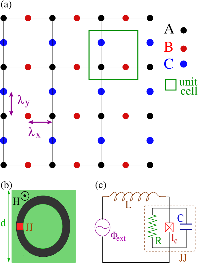
Figure 1: (Color online) (a) Schematic of a Lieb lattice; each unit cell (green square) has a corner SQUID (black) and two edge SQUIDs (red and blue). The nearest-neighbor coupling coefficients are indicated as $\lambda_{x}$ and $\lambda_{y}$; (b) Schematic of a single SQUID; (c) Equivalent electrical circuit for a dissipative-driven SQUID.

II Flux Dynamics Equations

Consider the Lieb lattice of Fig. 1a, in which each site is occupied by a SQUID (Fig. 1b) modelled by the equivalent circuit shown in Fig. 1c; all the SQUIDs are identical, with each of them featuring a self-inductance $L$, a capacitance $C$, a resistance $R$, and a critical current of the Josephson junction $I_{c}$. The SQUIDs are magnetically coupled to their nearest-neighbors along the horizontal (vertical) direction through their mutual inductance $M_{x}$ ($M_{y}$). Assuming that the current in each SQUID is given by the resistively and capacitively shunted junction ($RCSJ$) model Likharev1986 , the dynamic equations for the fluxes through the loops of the SQUIDs are Lazarides2017

$$LC\frac{d^{2}\Phi_{n,m}^{A}}{dt^{2}}+\frac{L}{R}\frac{d\Phi_{n,m}^{A}}{dt}+LI_{c}\sin\left(2\pi\frac{\Phi_{n,m}^{A}}{\Phi_{0}}\right)+\Phi_{n,m}^{A}$$

$$=\lambda_{x}\left(\Phi_{n,m}^{B}+\Phi_{n-1,m}^{B}\right)+\lambda_{y}\left(\Phi_{n,m}^{C}+\Phi_{n,m-1}^{C}\right)$$

$$+[1-2(\lambda_{x}+\lambda_{y})]\Phi_{e},$$ (1)

$$LC\frac{d^{2}\Phi_{n,m}^{B}}{dt^{2}}+\frac{L}{R}\frac{d\Phi_{n,m}^{B}}{dt}+LI_{c}\sin\left(2\pi\frac{\Phi_{n,m}^{B}}{\Phi_{0}}\right)+\Phi_{n,m}^{B}$$

$$=\lambda_{x}\left(\Phi_{n,m}^{A}+\Phi_{n+1,m}^{A}\right)+(1-2\lambda_{x})\Phi_{e},$$ (2)

$$LC\frac{d^{2}\Phi_{n,m}^{C}}{dt^{2}}+\frac{L}{R}\frac{d\Phi_{n,m}^{C}}{dt}+LI_{c}\sin\left(2\pi\frac{\Phi_{n,m}^{C}}{\Phi_{0}}\right)+\Phi_{n,m}^{C}$$

$$=\lambda_{y}\left(\Phi_{n,m}^{A}+\Phi_{n,m+1}^{A}\right)+(1-2\lambda_{y})\Phi_{e},$$ (3)

where $\Phi_{n,m}^{k}$ is the flux through the loop of the SQUID of kind $k$ in the $(n,m)$th unit cell ($k=A$, $B$, $C$, the notation is as in Fig. 1a), $I_{n,m}^{k}$ is the current in the SQUID of kind $k$ in the $(n,m)$th unit cell, $\Phi_{0}$ is the flux quantum, $\lambda_{x}=M_{x}/L$ ($\lambda_{y}=M_{y}/L$) is the coupling coefficient along the horizontal (vertical) direction, $t$ is the temporal variable, and $\Phi_{e}=\Phi_{ac}\,\cos(\omega t)$ is the external flux due to a sinusoidal magnetic field applied perpendicularly to the plane of the SLiMM. The subscript $n$ ($m$) runs from $1$ to $N_{x}$ ($1$ to $N_{y}$), so that $N=N_{x}\,N_{y}$ is the number of unit cells of the SLiMM (the number of SQUIDs is $3N$).

Using the relations $\tau=\omega_{LC}t$, $\phi_{n,m}^{k}={\Phi_{n,m}^{k}}/{\Phi_{0}}$, and $\phi_{ac}={\Phi_{ac}}/{\Phi_{0}}$, where $\omega_{LC}={1}/{\sqrt{LC}}$ is the inductive-capacitive ($LC$) SQUID frequency, Eqs. (II)-(II) can be normalized as

$${\cal L}\phi_{n,m}^{A}=\lambda_{x}\left(\phi_{n,m}^{B}+\phi_{n-1,m}^{B}\right)+\lambda_{y}\left(\phi_{n,m}^{C}+\phi_{n,m-1}^{C}\right)$$

$$+[1-2(\lambda_{x}+\lambda_{y})]\phi_{e}(\tau),$$ (4)

$${\cal L}\phi_{n,m}^{B}=\lambda_{x}\left(\phi_{n,m}^{A}+\phi_{n+1,m}^{A}\right)+(1-2\lambda_{x})\phi_{e}(\tau),$$ (5)

$${\cal L}\phi_{n,m}^{C}=\lambda_{y}\left(\phi_{n,m}^{A}+\phi_{n,m+1}^{A}\right)+(1-2\lambda_{y})\phi_{e}(\tau),$$ (6)

where

$$\beta=\frac{L\,I_{c}}{\Phi_{0}}=\frac{\beta_{L}}{2\pi}~{}~{}~{}{\rm and}~{}~{}~{}\gamma=\omega_{LC}\frac{L}{R}$$ (7)

is the SQUID parameter and the dimensionless loss coefficient, respectively, $\phi_{e}(\tau)=\phi_{ac}\cos(\Omega\tau)$ is the external flux of frequency $\Omega={\omega}/{\omega_{LC}}$ and amplitude $\phi_{ac}$, and $\cal L$ is an operator such that

$${\cal L}\phi_{n,m}^{k}=\ddot{\phi}_{n,m}^{k}+\gamma\dot{\phi}_{n,m}^{k}+\phi_{n,m}^{k}+\beta\sin\left(2\pi\phi_{n,m}^{k}\right).$$ (8)

The overdots on $\phi_{n,m}^{k}$ denote differentiation with respect to $\tau$.

The SQUID parameter and the loss coefficient used in the simulations have been chosen to be the same as those provided in the Supplemental Material of Ref. Zhang2015 for a $11\times 11$ SQUID metamaterial, i.e., $\beta_{L}=0.86$ and $\gamma=0.01$. These values result from Eq. (7) with $L=60~{}pH$, $C=0.42~{}pF$, $I_{c}=4.7~{}\mu A$, and subgap resistance $R=500$ Ohms. The value of the coupling between neighboring SQUIDs has been chosen to be $\lambda_{x}=\lambda_{y}=-0.02$, as it has been estimated for a $27\times 27$ SQUID metamaterial in the experiments of Ref. Trepanier2013 . These experiments were performed with a specially designed set up which allows for the application of uniform ac driving and/or dc bias fluxes Trepanier2013 ; Zhang2015 as well as dc flux gradients Trepanier2017 to the SQUID metamaterials which are placed into a waveguide. In the simulations in the next Sections, the described effects can be identified within the experimentally accessible range of $\phi_{ac}$ which spans the interval $0.001-0.1$ Zhang2015 . Furthermore, the SLiMM is chosen to have $16\times 16$ unit cells, so that its size is comparable with that of the $27\times 27$ SQUID metamaterial investigated in Refs. Trepanier2013 ; Trepanier2017 .

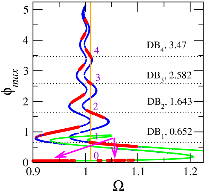
Figure 2: (Color online) The snaking flux amplitude $\phi_{max}$ - driving frequency $\Omega$ curve for a single SQUID with $\beta_{L}=0.86$ and $\phi_{ac}=0.05$ (blue curves). The green curves are calculated from Eq. (10). The vertical orange line is at frequency $\Omega=1.01$. The red symbols superposed on some branches of the $\phi_{max}$ - $\Omega$ curve, are the amplitudes of stable dissipative discrete breather families (except the ones indicated by the arrows, see text).

III Single SQUID Resonance and Multistable Dissipative Breathers

In a single SQUID driven with a relatively high amplitude field $\phi_{ac}$, strong nonlinearities shift the resonance frequency from $\Omega=\Omega_{SQ}$ to $\Omega\sim 1$, i.e., to the $LC$ frequency $\omega_{LC}$. Moreover, the curve for the oscillation amplitude of the flux through the loop of the SQUID $\phi_{max}$ as a function of the driving frequency $\Omega$ (SQUID resonance curve), aquires a snaking form as that shown in Fig. 2 (blue) Hizanidis2016a . That curve is calculated from the normalized single SQUID equation

$$\ddot{\phi}+\gamma\dot{\phi}+\beta\sin\left(2\pi\phi\right)+\phi=\phi_{ac}\cos(\Omega\tau),$$ (9)

for the flux $\phi$ through the loop of the SQUID. The curve ”snakes” back and forth within a narrow frequency region via succesive saddle-node bifurcations (occuring at those points for which $d\Omega/d\phi_{max}=0$). The many branches of the resonance curve have been traced numerically using Newton’s method; the stable branches are those which are partially covered by the red circles. An approximation to the resonance curve for $\phi_{max}\ll 1$ is given by Hizanidis2016a

$$\Omega^{2}=\Omega_{SQ}^{2}\pm\frac{\phi_{ac}}{\phi_{max}}$$

$$-\beta_{L}\phi_{max}^{2}\{a_{1}-\phi_{max}^{2}[a_{2}-\phi_{max}^{2}(a_{3}-a_{4}\phi_{max}^{2})]\},$$ (10)

where $a_{1}=\pi^{2}/2$, $a_{2}=\pi^{4}/12$, $a_{3}=\pi^{6}/144$, and $a_{4}=\pi^{8}/2880$, which implicitly provides $\phi_{max}(\Omega)$. The approximate curves Eq. (10) are shown in Fig. 2 in green color; they show excellent agreement with the numerical snaking resonance curve for $\phi_{max}\lesssim 0.6$. The vertical orange segment at $\Omega=1.01$ intersects the resonance curve at several $\phi_{max}$ points; five of those, numbered on Fig. 2 with consecutive integers from $0$ to $4$, correspond to stable solutions of the single SQUID equation. These five (5) solutions, which can be denoted as $(\phi_{i},\dot{\phi_{i}})$ with $i=0,1,2,3,4$, are used for the construction of four (4) trivial dissipative DB configurations. Note that the flux amplitude $\phi_{max}$ of these five solutions increases with increasing $i$. For constructing a (single-site) trivial dissipative DB, two simultaneously stable solutions are first identified, say $(\phi_{0},\dot{\phi_{0}})$ ($0$) and $(\phi_{1},\dot{\phi_{1}})$ ($1$), with low and high flux amplitude $\phi_{max}$, respectively. Then, one of the SQUIDs at $(n,m)=(n_{e}=N_{x}/2,m_{e}=N_{y}/2)$ (hereafter referred to as the central DB site, which also determines the location of the DB) is set to the high amplitude solution $1$, while all the other SQUIDs of the SLiMM (the background) are set to the low amplitude solution $0$. In order to numerically obtain a dissipative DB, that trivial DB configuration is used as initial condition for the time-integration of Eqs. (II)-(6); then, a stable dissipative DB (denoted as DB₁) is formed after integration for a few thousand time units. Three (3) more trivial dissipative DBs can be constructed similarly, e.g. by setting the central DB site to the solution $2$, $3$, or $4$, and the background to the solution $0$. Then, by integrating Eqs. (II)-(6) using as initial conditions these trivial DB configurations, three more stable dissipative DBs are obtained numerically (denoted as DB₂, DB₃, and DB₄, respectively). These four dissipative DBs are simultaneously stable and oscillate with the driving frequency $\Omega=1.01$.

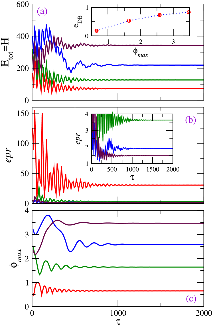
Figure 3: (Color online) (a) The total energy $E_{tot}=H$ of the SQUID Lieb metamaterial as a function of $\tau$ for $N_{x}=N_{y}=16$, $\beta_{L}=0.86$, $\lambda_{x}=\lambda_{y}=-0.02$, $\gamma=0.01$, $\Omega=1.01$, $\phi_{ac}=0.05$, and four (4) initial conditions - trivial breather configurations. Inset: The ratio $e_{DB}\equiv H_{n=n_{e},m=m_{e}}/H$ as a function of the steady-state dissipative breather amplitude $\phi_{max}$ for the four multistable dissipative breathers. The blue-dotted curve is a guide to the eye. (b) The energetic participation ratio $\it epr$ as a function of $\tau$ for the four initial conditions - trivial breather configurations. Inset: The $\it epr$ as a function of $\tau$ for the trivial breather configurations leading to the three more localized dissipative breathers. (c) The amplitude of the four multistable dissipative breathers $\phi_{max}$ as a function of $\tau$. The asymptotic values of $\phi_{max}$ have been used in the inset in (a).

The Hamiltonian (total energy) for the SLiMM descibed by Eqs. (II)-(6) for $\gamma=0$ is given by

$$H=\sum_{n,m}H_{n,m},$$ (11)

where the Hamiltonian (energy) density, $H_{n,m}$, is

$$H_{n,m}=\frac{\pi}{\beta}\sum_{k}\left[\left(q_{n,m}^{k}\right)^{2}+\left(\phi_{n,m}^{k}-\phi_{e}\right)^{2}\right]$$

$$-\sum_{k}\cos\left(2\pi\phi_{n,m}^{k}\right)$$

$$-\frac{\pi}{\beta}\{\lambda_{x}[(\phi_{n,m}^{A}-\phi_{e})(\phi_{n-1,m}^{B}-\phi_{e})$$

$$+2(\phi_{n,m}^{A}-\phi_{e})(\phi_{n,m}^{B}-\phi_{e})$$

$$+(\phi_{n,m}^{B}-\phi_{e})(\phi_{n+1,m}^{A}-\phi_{e})]$$

$$+\lambda_{y}[(\phi_{n,m}^{A}-\phi_{e})(\phi_{n,m-1}^{C}-\phi_{e})$$

$$+2(\phi_{n,m}^{A}-\phi_{e})(\phi_{n,m}^{C}-\phi_{e})$$

$$+(\phi_{n,m}^{C}-\phi_{e})(\phi_{n,m+1}^{A}-\phi_{e})]\},$$ (12)

where $q_{n,m}^{k}=\frac{d\phi_{n,m}^{k}}{d\tau}$ is the normalized instantaneous voltage across the Josephson junction of the SQUID in the $(n,m)$th unit cell of kind $k$. Both $H$ and $H_{n,m}$ are normalized to the Josephson energy, $E_{J}$. Two more quantities are also defined; the energetic participation ratio deMoura2003 ; Laptyeva2012

$$epr=\left[\sum_{n,m}\left(\frac{H_{n,m}}{H}\right)^{2}\right]^{-1},$$ (13)

which is a measure of localization (it roughly measures the number of the most strongly excited unit cells), and the complex synchronization parameter

$$\Psi=\frac{1}{3N}\sum_{n,m,k}e^{2\pi i\phi_{n,m}^{k}},$$ (14)

which is a spacially global measure of synchronization for coupled oscillators; its magnitude $r(\tau)=|\Psi(\tau)|$ ranges from zero (completely desynchronized solution) to unity (completely synchronized solution).

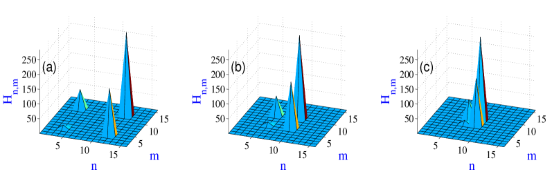
Figure 4: (Color online) The energy density $H_{n,m}$ of the SQUID Lieb metamaterial on the $n-m$ plane, in which four dissipative breathers exist simultaneously, for $N_{x}=N_{y}=16$, $\beta_{L}=0.86$, $\gamma=0.01$, $\lambda_{x}=\lambda_{y}=-0.02$, $\Omega=1.01$, $\phi_{ac}=0.05$, and different separations. The central breather sites for DB₁, DB₂, DB₃, and DB₄, are located on a square with vertices respectively at (a) $(n_{e},m_{e})=(4,4),~{}(4,12),~{}(12,4),~{}(12,12)$; (b) $(n_{e},m_{e})=(6,6),~{}(6,10),~{}(10,6),~{}(10,10)$; (c) $(n_{e},m_{e})=(7,7),~{}(7,9),~{}(9,7),~{}(9,9)$.

Eqs. (II)-(6) implemented with periodic boundary conditions are initialized with the four trivial breather configurations and then integrated in time with a standard Runge-Kutta fourth order scheme. The temporal evolution of the total energy $H$ of the SLiMM, the energetic participation ratio $epr$, and the dissipative DB amplitude $\phi_{max}$ are shown for all cases in Fig. 3. After some oscillations during the initial stages of evolution, all curves flatten indicating that a steady state has been reached (after $\sim 1500$ time units of integration). As it can be observed, the SLiMM has higher energy for higher amplitude DBs $\phi_{max}$ (Fig. 3a). The steady-state values of $\phi_{max}$ for the four DBs can be seen in Fig. 3c; these values have been also used in the inset of Fig. 3a. In that inset, the ratio of the energy of the unit cell to which the central DB site belongs over the total energy of the SLiMM, i.e., $e_{DB}=H_{n_{e},m_{e}}/H$, is shown for the four DBs. This ratio increases considerably with increasing DB amplitude. This is certainly compatible with Fig. 3b (see also the inset), in which $epr$ is plotted as a function of $\tau$, where apparently higher amplitude DBs provide more localized structures than lower amplitude ones.

It is convenient to present the energy density $H_{n,m}$ profiles of the four dissipative DBs in one plot, as shown in Fig. 4. These profiles are obtained after $2000~{}T\simeq 12500$ time units of integration ($T=2\pi/\Omega$) using an appropriate initial condition which is a combination of the four trivial DB configurations. The difference between the three subfigures is in the distances between the central DB sites. Remarkably, the steady-state total energy of the SLiMM, $H=E_{tot}$, is the same in all the three cases and equal to $H=580.6$, indicating that the interaction between these DBs is almost negligible, even if they are located very closely (as in Fig. 4c).

IV Bifurcations of Multistable Dissipative Breathers

In this Section, the parameter intervals in which these four DBs are stable are determined; for this purpose, the steady-state DB amplitudes $\phi_{max}$ are calculated as a function of either the driving field amplitude $\phi_{ac}$, or the magnitude of the coupling coefficients for isotropic coupling $\lambda_{x}=\lambda_{y}$, or the driving frequency $\Omega$. First, $\phi_{max}$, the energetic participation ratio $epr$, and the magnitude of the synchronization parameter averaged over the steady-state integration time $\tau_{int}=2000~{}T$ time units (transients have been discarded), are calculated as a function of $\phi_{ac}$ (Fig. 5). In Fig. 5a, it can be seen that higher amplitude DBs remain stable for narrower intervals of $\phi_{ac}$. Interestingly, higher amplitude DBs may turn into lower amplitude ones even several times until they completely dissapear. As an example, we note that $DB_{4}$ (blue curve) which is stable approximately for $\phi_{ac}$ between $0.04$ and $0.085$, it transforms to a $DB_{2}$ for $\phi_{ac}<0.04$, and then to an even lower amplitude DB at $\phi_{ac}<0.015$. The presence of the latter DB is rather unexpected, since it cannot be identified with one the four DB families under consideration. All the DBs disappear for $\phi_{ac}\lesssim 0.005$, since the nonlinearity is not strong enough to localize energy in the SLiMM. For $\phi_{ac}$ exceeding a critical value, which is higher for lower amplitude DBs (e.g., $0.085$ for $DB_{4}$ and $0.118$ for $DB_{1}$), all the four DBs turn into irregular multibreather states.

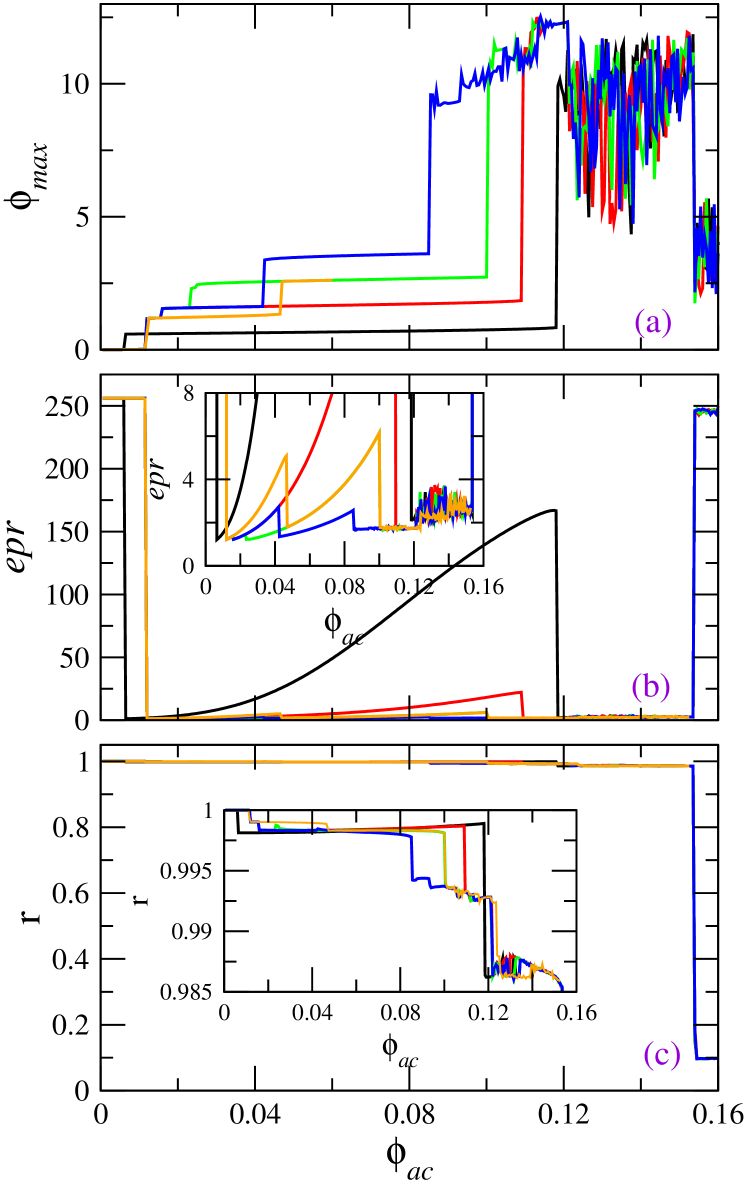
Figure 5: (Color online) (a) The four dissipative breather amplitudes $\phi_{max}$ as a function of the driving field amplitude $\phi_{ac}$, for $N_{x}=N_{y}=16$, $\beta_{L}=0.86$, $\gamma=0.01$, $\Omega=1.01$, and $\lambda_{x}=\lambda_{y}=-0.02$. (b) The corresponding energetic participation ratios $epr$ as a function of $\phi_{ac}$. Inset: Enlargement for low $epr$ values. (c) The corresponding magnitudes of the synchronization parameter averaged over the steady-state integration time $<r>_{int}$ as a function of $\phi_{ac}$. Inset: Enlargement for values of $<r>_{int}\lesssim 1$.

In Figs. 5b and 5c the corresponding $epr$ and $<r>_{int}$ are presented as a function of $\phi_{ac}$. In Fig. 5b, it can be seen that when all the DBs dissapear for low $\phi_{ac}$, the SLiMM reaches a homogeneous state which is advocated by the large, close to the maximum possible value of $epr\simeq N=256$. In that case, $<r>_{int}$ is exactly unity (Fig. 5c) since the homogeneous state is synchronized. For high values of $\phi_{ac}$ ($>0.118$), where $\phi_{max}$ for all the four DBs varies irregularly with varying $\phi_{ac}$, the value of $epr$ can be used to distinguish between two different regimes: the first one from $\phi_{ac}\simeq 0.118$ to $0.154$, in which the low, fluctuating value of $epr$ suggests the existence of (possibly chaotic) multibreathers (see also the inset of Fig. 5b), and the second from $\phi_{ac}\simeq 0.154$ to $0.16$, in which the high value of $epr$ ($\simeq 256$) suggests the existence of a desynchronized state in which all the units cells are excited. For intermediate values of $\phi_{ac}$, $epr$ generally increases with increasing $\phi_{ac}$; in particular, for DB₁ it increases to rather high values because of the relative enhancement of the oscillation amplitude of the background unit cells with respect to the central DB unit cell. However, this is not observed for the high amplitude DBs, for which the increase is either moderate (DB₂) or very small (DB₃, DB₄). It is also apparent that whenever a DB is tranformed to another, a small jump in $epr$ occurs (inset). Fig. 5c provides useful information on the synchronization of the various SLiMM states. For example, for $\phi_{ac}\simeq 0.154$ to $0.16$, $<r>_{int}$ falls off to very low values indicating desynchronization as mentioned above. For the values of $\phi_{ac}$ which provide stable single-site DBs that belong to one of the four (4) families (as well as the fifth one which has appeared), the measure $<r>_{int}$ is always very close to unity (inset); that occurs because all the ”background” SQUIDs are oscillating in phase with the same amplitude, and only one SQUID (the central DB site) is oscillating with higher amplitude and opposite phase with respect to the others. For low $\phi_{ac}$, the SLiMM reaches a homogeneous state (the DBs have dissapeared) and then $<r>_{int}$ is exactly unity.

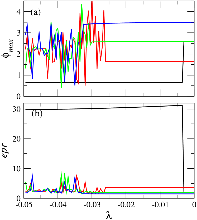
Figure 6: (Color online) (a) The four dissipative breather amplitudes $\phi_{max}$ as a function of the coupling coefficients in the case of isotropic coupling, $\lambda=\lambda_{x}=\lambda_{y}$, for $N_{x}=N_{y}=16$, $\beta_{L}=0.86$, $\gamma=0.01$, $\Omega=1.01$, and $\phi_{ac}=0.05$. (b) The corresponding energetic participation ratios $epr$ as a function of $\lambda$.

The corresponding diagram of the DB flux amplitudes $\phi_{max}$ as a function of the coupling coefficients for isotropic coupling $\lambda=\lambda_{x}=\lambda_{y}$ is shown in Fig. 6. Remarkably, the four DBs maintain their amplitudes almost constant for a substantial interval of $\lambda$ (Fig. 6a), i.e., from $\lambda=0$ to $-0.026$ which includes the estimated physically acceptable values for that system Trepanier2013 ; Trepanier2017 . The corresponding values of the $epr$ remain low, except for the lowest amplitude breather (DB₁), for which $epr\simeq 30$. Note that DB₁ dissapears for $\lambda>-0.003$ but it exists all the way down to $\lambda=-0.05$. For large magnitudes of $\lambda$, the amplitudes of the three high amplitude breathers (DB₂, DB₃, DB₄) vary irregularly with varying $\lambda$; however, as it can be observed in Fig. 6b, their $epr$ remains relatively low, indicating the spontaneous formation of multibreathers.

The bifurcation diagram of the DB amplitudes $\phi_{max}$ as a function of the driving frequency $\Omega$ is particularly interesting. This diagram has been superposed on the single SQUID resonance curve shown in Fig. 2 as red circles. Notice that DB flux amplitudes (red circles) are very close to the corresponding flux amplitudes of single-SQUID stable solutions (which are covered by the red circles). All red-circled branches (except the lowest ones pointed by the arrows) correspond to stable DB families. The red-cirled branches indicated by the arrows correspond to almost homogeneous solutions which are not DBs. Note that different number of multistable dissipative DBs exists for different driving frequencies, depending on the broadness of the red-circled branches; for example, for $\Omega=1.01$ there are four simultaneously stable DBs, while for $\Omega=1.03$ there are two, and for $\Omega=1.07$ there is only one stable DB.

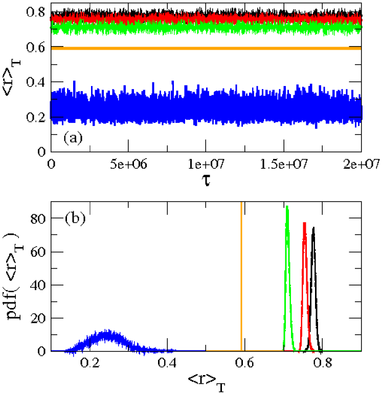
Figure 7: (Color online) (a) The synchronization parameter averaged over the driving period $T$, $<r>_{T}$, as a function of $\tau$ for $N_{x}=N_{y}=16$, $\beta=0.86$, $\gamma=0.01$, $\lambda_{x}=\lambda_{y}=-0.02$, $\phi_{ac}=0.1$, and $\Omega=1.01$ (black); $\Omega=1.02$ (red);$\Omega=1.03$ (green);$\Omega=1.04$ (blue); $\Omega=1.05$ (orange). (b) The corresponding probability distribution functions for the values of $<r>_{T}$, normalized to unity area. The actual peak of the orange curve, which is practically a $\delta-$function is at $pdf(<r>_{T})=8000$.

V Novel Dynamic SLiMM States

So far, we focused on the formation of single-site, dissipative DBs in a SLiMM, which can be generated through trivial DB configurations, and they are simultaneously stable. Beyond dissipative DB solutions, other interesting numerical solutions have been obtained; these solutions correspond to counter-intuitive dynamic states such as the so-called chimera states and a type of states that exhibit spatial homogeneity as well as chaotic evolution. Typical examples of such states, whose analysis requires futher work, are demonstrated here. First, a chimera state solution is illustrated which is generated from the following initial condition

$$\phi_{n,m}^{k}(\tau=0)=\left\{\begin{array}[]{ll}0.5,&\mbox{if~{}}N_{x}/4+1<n\leq 3N_{x}/4\\ &\mbox{and~{}}N_{y}/4+1<m\leq 3N_{y}/4;\\ 0,&\mbox{otherwise ,}\end{array}\right.$$ (18)

$$\dot{\phi}_{n,m}^{k}(\tau=0)=0,\mbox{for any $n$, $m$}.$$ (19)

With Eqs. (18) and (19) as initial conditions, Eqs. (II)-(6) for the SLiMM are integrated in time. The magnitude of the synchronization parameter averaged over each driving period $T=2\pi/\Omega$, $<r>_{T}(\tau)$, is monitored in time and the results are shown in Fig. 7a for five different driving frequencies $\Omega$ close to unity. It can be seen that $<r>_{T}(\tau)$ is in all cases considerably less than unity, indicating significant desynchronization. The fluctuations, however, of $<r>_{T}(\tau)$ do not all have the same size. Specifically, for $\Omega=1.01$, $1.015$, and $1.02$ (black, red, and green curves, respectively), the fluctuations have roughly the same size. For $\Omega=1.025$ (blue curve), the size of fluctuations is significantly higher, while for $\Omega=1.03$ (orange curve) the fluctuations are practically zero. This can be seen more clearly in Fig. 7b, in which the distributions $pdf(<r>_{T})$ of the values of $<r>_{T}(\tau)$ are shown; the full-width half-maximum (FWHM) of the $pdf(<r>_{T})$s, quantifies the level of metastability of chimera states Shanahan2010 ; Lazarides2015a . A partially desynchronized dynamic state (i.e., with $<r>_{T}<1$ but practically zero fluctuations), is not a chimera state but a clustered state, i.e., a non-homogeneous state in which different groups of SQUIDs oscillate with different amplitudes and phases with respect to the driving field; however, the SQUID oscillators that belong to the same group are synchronized. Thus, as can be inferred from Fig. 7 as well as by the inspection of the flux profiles at the end of integration time (not shown), the curves for $\Omega=1.01$, $1.015$, $1.02$, and $1.025$ (black, red, green, and blue curves, respectively), are indeed due to chimera states. The energy density profiles at the end of the integration time for $\Omega=1.01$, $1.03$, and $1.05$, are shown in Fig. 8. The first two are typical for chimera states, while the last one is typical for a clustered state. Note that the SQUIDs within the square in which the fluxes were initialized to a non-zero value, oscillate with high amplitude and they are not synchronized. The rest of the SQUIDs, i.e., outside that square, oscillate in phase and with the same (low) amplitude. Thus, from the initial condition Eqs. (18) and (19), different chimera states are obtained for different driving frequencies. These states differ in their asymptotic value of $<r>_{T}$ as well as the FWHM of their $pdf(<r>_{T})$s which determines their metastability level. In Fig. 8c, on the other hand, one may distinguish easily groups of SQUIDs with the same amplitude. The SQUIDs that belong to such a group are synchronized together while the groups are not synchronized to each other. In this clustered state, all the SQUIDs are oscillating with high amplitude (note the energy scales).

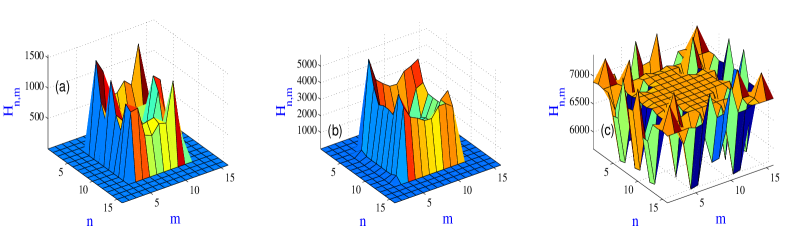
Figure 8: (Color online) The energy density $H_{n,m}$ of the SQUID Lieb metamaterial (energy per unit cell) on the $n-m$ plane, after integrating the dynamic equations for $10^{7}~{}T$ time units, for $N_{x}=N_{y}=16$, $\beta_{L}=0.86$, $\gamma=0.01$, $\lambda_{x}=\lambda_{y}=-0.02$, $\phi_{ac}=0.1$, and (a) $\Omega=1.01$; (b) $\Omega=1.03$; (c) $\Omega=1.05$. The value of the synchronization parameter averaged over the steady-state integration time is $<r>_{int}\sim 0.77$, $\sim 0.71$, $\sim 0.59$, respectively.

Figure 9: (Color online) (a) The flux oscillation amplitudes $\phi_{max}^{A}$, $\phi_{max}^{B}$, and $\phi_{max}^{C}$ of the SQUIDs of kind $A$ (blue), $B$ (red), and $C$ (green), respectively, of the $(n_{e},m_{e})$th unit cell as a function of the driving field amplitude $\phi_{ac}$ for $N_{x}=N_{y}=16$, $\beta_{L}=0.86$, $\gamma=0.01$, $\Omega=1.01$, and $\lambda_{x}=\lambda_{y}=-0.02$. Inset: The magnitude of the synchronization parameter averaged over the steady-state integration time $<r>_{int}$ (red) and the total energy of the SQUID Lieb metamaterial divided by $E_{0}$, $E_{tot}/E_{0}$ (blue), as a function of $\phi_{ac}$. Note the large hysteresis region in those curves. (b) Time-dependence of $\phi^{A}$ (blue), $\phi^{B}$ (red), and $\phi^{C}$ (green), for $\phi_{ac}=0.2$ and the other parameters as in (a). (c) The fluxes $\phi^{A}$ (green), $\phi^{B}$ (red), and $\phi^{C}$ (blue), on the $n-m$ plane for $\phi_{ac}=0.2$ and the other parameters as in (a). (d) Stroboscopic plots of $\phi^{C}(nT)-q^{C}(nT)$, with $q^{C}\equiv\dot{\phi}^{C}$, for $\phi_{ac}=0.1$ (blue) and $\phi_{ac}=0.2$ (red). An enlargement of the period-1 attractor is shown in the inset. The red arrows are along the transient leading to the chaotic attractor.

A family of novel solutions emerges through an order-to-chaos phase transition that is demonstrated for varying $\phi_{ac}$. Eqs. (II)-(6) with periodic boundary conditions are integrated in time for $\phi_{ac}$ increasing from zero to higher values; the initial condition is homogeneous, i.e., $\phi_{n,m}^{k}(\tau=0)=\dot{\phi}_{n,m}^{k}(\tau=0)=0$ for any $n$, $m$, and $k$. The flux field amplitude $\phi_{ac}$ increases in small steps, and for each step the solution for the previous step is taken as the initial condition. For relatively low $\phi_{ac}$, the amplitudes of the oscillating fluxes through the loops of the SQUIDs have low values and they are very close to each other, i.e., $\phi_{max}^{A}\simeq\phi_{max}^{B}=\phi_{max}^{C}$ as shown in Fig. 9a (all the SQUIDs of kind $k$ are oscillating with amplitude $\phi_{max}^{k}$, $k=A,B,C$). Actually, the difference between $\phi_{max}^{A}$ and $\phi_{max}^{B,C}$ is less than $1\%$ in this regime. Moreover, the fluxes in all kinds of SQUIDs are oscillating periodically in phase, and thus the degree of synchronization $<r>_{int}$ of these states is almost unity (see the upper branch of the red curve in the inset of Fig. 9a). That state is referred to as an almost homogeneous state in space. In the inset of Fig. 9a, the total energy of the SLiMM $E_{tot}$ divided by $E_{0}=10^{6}$ is plotted as a function of $\phi_{ac}$; that energy increases smoothly with increasing $\phi_{ac}$ (lower branch of the blue curve in the inset of Fig. 9a). At a critical value of $\phi_{ac}$, $\phi_{ac}^{c}\simeq 0.155$, the situation changes drastically, as an abrupt increase of all the amplitudes $\phi_{max}^{k}$ occurs while their values become considerably different ($\phi_{max}^{A}$ attains considerably larger values than $\phi_{max}^{B}=\phi_{max}^{C}$). Moreover, for $\phi_{ac}>\phi_{ac}^{c}$, the values of $\phi_{max}^{k}$s vary irregularly with increasing $\phi_{ac}$, although their average values as well as the difference between $\phi_{max}^{A}$ and $\phi_{max}^{B,C}$ increase (Fig. 9a). Also, at the phase transition point $\phi_{ac}^{c}$, the parameter $<r>_{int}$ abruptly jumps to a value which indicates significant desynchronization, $<r>_{int}\sim 0.7$; that value remains almost unchanged with further increasing $\phi_{ac}$ (inset). The variation of the total energy of the SLiMM $E_{tot}$ is similar to that of the variation of the $\phi_{max}^{k}$, i.e., it jumps abruptly to higher value at $\phi_{ac}=\phi_{ac}^{c}$ (inset). Recall that the above remarks hold for $\phi_{ac}$ increasing from zero to higher values. The corresponding curves for $<r>_{int}$ and $E_{tot}$ for $\phi_{ac}$ decreasing from $0.3$ to zero are also shown in the inset of Fig. 9a (lower branch of the red curve and upper branch of the blue curve, respectively). The ”explosive” (first-order) character of the transition is clearly manifested by the presence of a large hysteresis region.

Consider again the case in which $\phi_{ac}$ increases from zero to higher values. In that case, the steady-states of the SLiMM are almost synchronized (almost spatially homogeneous) and temporally periodic for $\phi_{ac}<\phi_{ac}^{c}$. Note however that those states are exactly homogeneous at the unit cell level, i.e., that $\bar{\phi}_{n,m}=\sum_{k}{\phi}_{n,m}^{k}=c$ for any $n$ and $m$, with $c$ being a constant. For $\phi_{ac}>\phi_{ac}^{c}$ the SLiMM states acquire chaotic time-dependence, while they retain partial homogeneity and thus synchronization; that is, all the SQUIDs of kind $k$ are synchronized although they execute chaotic oscillations. Remarkably, at the unit cell level, even this state is spatially homogeneous. In Fig. 9b the time-dependence of the fluxes $\phi^{A}$, $\phi^{B}$, and $\phi^{C}$ (identical for all the SQUID of kind $A$, $B$, and $C$, respectively, of the SLiMM) are plotted for $\phi_{ac}=0.2$ during a few thousands time-units. Apparently, the flux oscillations are irregular, indicating chaotic behavior which has been checked to persists for very long times (note that $\phi^{B}=\phi^{C}$ due to the isotropic coupling). A flux profile for that state is shown in Fig. 9c, in which the spatial homogeneity within each sublattice of the SLiMM is apparent. Thus, large scale synchronization between oscillators in a chaotic state occurs in this case. In Fig. 9d, two stroboscopic plots in the reduced $\phi^{C}$ - $\dot{\phi}^{C}$ ($\dot{\phi}^{C}=q^{C}$) phase space are shown together for the $C$ SQUID at the $(n_{e},m_{e})$th unit cell. In the first one (blue down-triangles, inset), the SLiMM is in an almost synchronized temporally periodic state ($\phi_{ac}=0.1$); in the the second one (red circles), the SLiMM is in a partially synchronized (synchronization of the SQUIDs within each sublattice) temporally chaotic state ($\phi_{ac}=0.2$). Apparently, the trajectory in the reduced phase-space tends to a point in the former case, while it tends to a large area attractor in the latter. In Fig. 9d, the transients leading the trajectories to the one or the other attractor are also shown.

VI Conclusions

The existence of several regions in parameter space in which simultaneously stable dissipative DBs in a dissipative SLiMM which is driven by a sinusoidal flux field has been demonstrated numerically. For that purpose, the dynamic equations Eqs. (II)-(6) for the fluxes threading the loops of the SQUIDs are integrated in time with periodic boundary conditions. The initial conditions have been properly designed to provide trivial DB configurations using combinations of simultaneously stable solutions of the single-SQUID oscillator. For substantial nonlinearity excited from a flux field with relatively high amplitude, the single-SQUID resonance curve exhibits several simultaneously stable solutions at frequencies around resonance. That allows for the construction of several trivial DB configurations at some particular frequency; the subsequent temporal evolution through Eqs. (II)-(6) results in multistable (co-existing) dissipative DBs. The bifucation diagrams for the calculated DB amplitudes as a function of $\phi_{ac}$, $\lambda$, and $\Omega$ have been presented, which reveal that multistability persists within substantial parameter intervals. For a better interpretation of those bifurcation diagrams, well-established measures for energy localization and synchronization of oscillators in discrete lattices were defined, and they were calculated for each dissipative DB. Remarkably, the interactions between co-existing DBs are very weak; no appreciable change in the total energy of the SLiMM has been observed even when the co-existing DBs are very close together. The bifurcation diagram of the dissipative DB amplitudes as a function of $\Omega$, shown as the branches formed by the red circles in Fig. 2, resembles the snaking bifurcation curves for spatially localized states in the Swift-Hohenberg equation Knobloch2008 ; Bergeon2008 ; however, snaking bifurcation curves also occur in discrete problems Taylor2010 ; Prilepsky2012 ; Dean2015 . Interestingly, snaking bifurcation diagrams for chimera states have been obtained in the 1D extended Bogdanov-Takens lattice Clerc2016 .

Besides single-site multistable dissipative DBs, two other types of dynamic states were demonstrated; chimera states, which can be generated in a SLiMM by appropriate choice of initial conditions, and spatially homogeneous (at the unit cell level) - temporally chaotic states. The existence of the former have been demonstrated in 1D SQUID metamaterials, and the mechanism for their generation through the attractor crowding effect in coupled nonlinear oscillator arrays Wiesenfeld1989 ; Tsang1990 has been described Lazarides2015b ; Hizanidis2016a . Similar chimera states are also expected to appear in SQUID metamaterials on 2D tetragonal lattices. The spatially homogeneous - temporally chaotic states, however, are peculiar to the lattice geometry of the SLiMM, and indicate the wealth of dynamic behaviors that may be encountered in that system. As $\phi_{ac}$ increases from zero, the SLiMM passes through states which are spatially (almost) homogeneous and temporally periodic. At a critical value of $\phi_{ac}=\phi_{ac}^{c}$ a transition occurs, and for $\phi_{ac}>\phi_{ac}^{c}$ the SLiMM passes through states in which all the SQUIDs of kind $k$ (i.e., the SQUIDs within each sublattice) have the same amplitude and they are synchronized together, while their time-dependence is chaotic! These states exhibit large-scale chaotic synchronization Pecora1990 ; Heagy1994 ; notably, states with spatial coherence and temporal chaos have been obtained in coupled map lattices with asymmetric short-range couplings Aranson1992 . The order-to-chaos transition with hysteresis obtained here is similar to that demonstrated numerically and observed in laser-cooled trapped ions Hoffnagle1988 . When seen as a synchronization-desynchronization transition with hysteresis, it resembles the explosive first order transition to synchrony observed in electronic circuits Levya2012 .

References

- (1) S. M. Anlage, The physics and applications of superconducting metamaterials, J. Opt. 13, 024001 (2011).
- (2) P. Jung, A. V. Ustinov, and S. M. Anlage, Progress in superconducting metamaterials, Supercond. Sci. Technol. 27, 073001 (2014).
- (3) N. Lazarides and G. P. Tsironis, Superconducting metamaterials, arXiv preprint, arXiv:1710.00680 .
- (4) M. Lapine, M. Gorkunov, and K. H. Ringhofer, Nonlinearity of a metamaterial arising from diode insertions into resonant conductive element, Phys. Rev. E 67, 065601 (2003).
- (5) M. Lapine, I. V. Shadrivov, and Y. S. Kivshar, Colloquium: Nonlinear metamaterials, Rev. Mod. Phys. 86, 1093 (2014).
- (6) B. Josephson, Possible new effects in superconductive tunnelling, Phys. Lett. A 1, 251 (1962).
- (7) C. Du, H. Chen, and S. Li, Quantum left-handed metamaterial from superconducting quantum-interference devices, Phys. Rev. B 74, 113105 (2006).
- (8) N. Lazarides and G. P. Tsironis, rf superconducting quantum interference device metamaterials, Appl. Phys. Lett. 90, 163501 (2007).
- (9) P. Jung, S. Butz, S. V. Shitov, and A. V. Ustinov, Low-loss tunable metamaterials using superconducting circuits with Josephson junctions, Appl. Phys. Lett. 102, 062601 (2013).
- (10) S. Butz, P. Jung, L. V. Filippenko, V. P. Koshelets, and A. V. Ustinov, A one-dimensional tunable magnetic metamaterial, Opt. Express 21, 22540 (2013).
- (11) M. Trepanier, Daimeng Zhang, O. Mukhanov, and S. M. Anlage, Realization and modeling of rf superconducting quantum interference device metamaterials, Phys. Rev. X 3, 041029 (2013).
- (12) Daimeng Zhang, M. Trepanier, O. Mukhanov, and S. M. Anlage, Broadband transparency of macroscopic quantum superconducting metamaterials, Phys. Rev. X 5, 041045 (2015).
- (13) P. Jung, S. Butz, M. Marthaler, M. V. Fistul, J. Leppäkangas, V. P. Koshelets, and A. V. Ustinov, Multistability and switching in a superconducting metamaterial, Nat. Comms. 5, 3730 (2014).
- (14) M. Trepanier, Daimeng Zhang, O. Mukhanov, V. P. Koshelets, P. Jung, S. Butz, E. Ott, T. M. Antonsen, A. V. Ustinov, and S. M. Anlage, Coherent oscillations of driven rf SQUID metamaterials, Phys. Rev. E 95, 050201(R) (2017).
- (15) N. Lazarides, G. P. Tsironis, and M. Eleftheriou, Dissipative discrete breathers in rf SQUID metamaterials, Nonlinear Phenom. Complex Syst. 11, 250 (2008).
- (16) G. P. Tsironis, N. Lazarides, and I. Margaris, Wide-band tuneability, nonlinear transmission, and dynamic multistability in SQUID metamaterials, Appl. Phys. A 117, 579 (2014).
- (17) N. Lazarides, G. Neofotistos, and G. P. Tsironis, Chimeras in SQUID metamaterials, Phys. Rev. B 91, 054303 (2015).
- (18) J. Hizanidis, N. Lazarides, and G. P. Tsironis, Robust chimera states in SQUID metamaterials with local interactions, Phys. Rev. E 94, 032219 (2016).
- (19) Y. Kuramoto and D. Battogtokh, Coexistence of coherence and incoherence in nonlocally coupled phase oscillators, Nonlinear Phenom. Complex Syst. 5, 380 (2002).
- (20) M. J. Panaggio and D. M. Abrams, Chimera states: Coexistence of coherence and incoherence in network of coulped oscillators, Nonlinearity 28, R67 (2015).
- (21) N. Lazarides and G. P. Tsironis, SQUID metamaterials on a Lieb lattice: From flat-band to nonlinear localization, Phys. Rev. B 96, 054305 (2017).
- (22) R. A. Vicencio, C. Cantillano, L. Morales-Inostroza, B. Real, C. Mejía-Cortés, S. Weimann, A. Szameit, and M. I. Molina, Observation of localized states in Lieb photonic lattices, Phys. Rev. Lett. 114, 245503 (2015).
- (23) S. Mukherjee, A. Spracklen, D. Choudhury, N. Goldman, P. Öhberg, E. Andersson, and R. R. Thomson, Observation of a localized flat-band state in a photonic Lieb lattice, Phys. Rev. Lett. 114, 245504 (2015).
- (24) S. Flach and A. V. Gorbach, Discrete breathers - advances in theory and applications, Phys. Rep. 467, 1 (2008).
- (25) S. Flach, Discrete breathers in a nutshell, Nonlinear Theory and Its Applications, IEICE 3, 1 (2012).
- (26) R. S. MacKay and S. Aubry, Proof of existence of breathers for time - reversible or Hamiltonian networks of weakly coupled oscillators, Nonlinearity 7, 1623 (1994).
- (27) S. Aubry, Breathers in nonlinear lattices: Existence, linear stability and quantization, Physica D 103, 201 (1997).
- (28) P. Binder, D. Abraimov, A. V. Ustinov, S. Flach, and Y. Zolotaryuk, Observation of breathers in Josephson ladders, Phys. Rev. Lett. 84, 745 (2000).
- (29) E. Trías, J. J. Mazo, and T. P. Orlando, Discrete breathers in nonlinear lattices: Experimental detection in a Josephson array, Phys. Rev. Lett. 84, 741 (2000).
- (30) M. Sato, B. E. Hubbard, A. J. Sievers, B. Ilic, D. A. Czaplewski, and H. G. Graighead, Observation of locked intrinsic localized vibrational modes in a micromechanical oscillator array, Phys. Rev. Lett. 90, 044102 (2003).
- (31) J. Edler, R. Pfister, V. Pouthier, C. Falvo, and P. Hamm, Direct observation of self-trapped vibrational states in helices, Phys. Rev. Lett. 93, 106405 (2004).
- (32) U. T. Schwarz, L. Q. English, and A. J. Sievers, Experimental generation and observation of intrinsic localized spin wave modes in an antiferromagnet, Phys. Rev. Lett. 83, 223 (1999).
- (33) P. J. Martínez, L. M. Floría, F. Falo, and J. J. Mazo, Intrinsically localized chaos in discrete nonlinear extended systems, Europhys. Lett. 45, 444 (1999).
- (34) P. J. Martínez, M. Meister, L. M. Floria, and F. Falo, Dissipative discrete breathers: periodic, quasiperiodic, chaotic, and mobile, Chaos 13, 610 (2003).
- (35) J. L. Marín, F. Falo, P. J. Martínez, and L. M. Floría, Discrete breathers in dissipative lattices, Phys. Rev. E 63, 066603 (2001).
- (36) J. J. Mazo, Discrete Breathers in Two-Dimensional Josephson-Junction Arrays, Phys. Rev. Lett. 89, 234101 (2002).
- (37) J. J. Mazo and T. P. Orlando, Discrete breathers in Josephson arrays, Chaos 13, 733 (2003).
- (38) S. Flach and A. V. Gorbach, Discrete Breathers with Dissipation, Lect. Notes Phys. 751, 289-320 (2008).
- (39) N. Lazarides, M. Eleftheriou, and G. P. Tsironis, Discrete breathers in nonlinear magnetic metamaterials, Phys. Rev. Lett. 97, 157406 (2006).
- (40) J. L. Marín, J. C. Eilbeck, and F. M. Russell, Localized moving breathers in a 2D hexagonal lattice, Phys. Lett. A 248, 225 (1998).
- (41) J. L. Marín, F. M. Russell, and J. C. Eilbeck, Breathers in cuprate-like lattices, Phys. Lett. A 281, 21 (2001).
- (42) A. Fraile, E. N. Koukaras, K. Papagelis, N. Lazarides, and G.P. Tsironis, Long-lived discrete breathers in free-standing graphene, Chaos, Solitons Fractals 87, 262 (2016).
- (43) K. K. Likharev, Dynamics of Josephson Junctions and Circuits, Gordon and Breach, Philadelphia, 1986.
- (44) F. A. B. F. de Moura, M. D. Coutinho-Filho, E. P. Raposo, and M. L. Lyra, Delocalization in harmonic chains with long-range correlated random masses, Phys. Rev. B 68, 012202 (2003).
- (45) T. V. Laptyeva, J. D. Bodyfelt, and S. Flach, Subdiffusion of nonlinear waves in two-dimensional disordered lattices, Europhys. Lett. 98, 60002 (2012).
- (46) N. Lazarides and G. P. Tsironis, Nonlinear localization in metamaterials, In I. Shadrivov, M. Lapine, and Yu. S. Kivshar, editors, Nonlinear, Tunable and Active Metamaterials, pages 281–301. Springer International Publishing, Switzerland, 2015.
- (47) M. Shanahan, Metastable chimera states in community-structured oscillator networks, Chaos 20, 013108 (2010).
- (48) E. Knobloch, Spatially localized structures in dissipative systems: open problems, Nonlinearity 21, T45 (2008).
- (49) A. Bergeon, J. Burke, E. Knobloch, and I. Mercader, Eckhaus instability and homoclinic snaking, Phys. Rev. E 78, 046201 (2008).
- (50) A. D. Dean, P. C. Matthews, S. M. Cox, and J. R. King, Orientation-dependent pinning and homoclinic snaking on a planar lattice, SIAM J. Appl. Dyn. Syst. 14, 481 (2015).
- (51) C. Taylor and J. H.P. Dawes, Snaking and isolas of localised states in bistable discrete lattices, Phys. Lett. A 375, 14 (2010).
- (52) J. E. Prilepsky, A. V. Yulin, M. Johansson, and S. A. Derevyanko, Discrete solitons in coupled active lasing cavities, Opt. Lett. 37, 4600 (2012).
- (53) M. G. Clerc, S. Coulibaly, M. A. Ferré, M. A. García-Nustes, and R. G. Rojas, Chimera-type states induced by local coupling, Phys. Rev. E 93, 052204 (2016).
- (54) K. Wiesenfeld and P. Hadley Attractor crowding in oscillator arrays, Phys. Rev. Lett. 62, 1335 (1989).
- (55) Kwok Yeung Tsang and K. Wiesenfeld, Attractor crowding in Josephson junction arrays, Appl. Phys. Lett. 56, 495 (1990).
- (56) L. M. Pecora and T. L. Carroll, Synchronization in chaotic systems, Phys. Rev. Lett. 64, 821 (1990).
- (57) J. F. Heagy, T. L. Carroll, and L. M. Pecora, Synchronous chaos in coupled oscillator systems, Phys. Rev. E 50, 1874 (1994).
- (58) I. Aranson, D. Golomb, and H. Sompolinsky, Spatial coherence and temporal chaos in macroscopic systems with asymmetrical couplings, Phys. Rev. Lett. 68, 3495 (1992).
- (59) J. Hoffnagle, R. G. DeVoe, L. Reyna, and R. G. Brewer, Order-chaos transition of two trapped ions, Phys. Rev. Lett. 61, 255 (1988).
- (60) I. Leyva, R. Sevilla-Escoboza, J. M. Buldu, I. Sendina-Nadal, J. Gomez-Gardenes, A. Arenas, Y. Moreno, S. Gomez, R. Jaimes-Reategui, and S. Boccaletti, Explosive first-order transition to synchrony in networked chaotic oscillators, Phys. Rev. Lett. 108, 168702 (2012).
- (61) A. I. Maimistov and I. R. Gabitov, Nonlinear response of a thin metamaterial film containing Josephson junctions, Opt. Commun. 283, 1633-1639 (2010).
- (62) D. Zueco, C. Fernández-Juez, J. Yago, U. Naether, B. Peropadre, J. J. García-Ripoll, and J. J. Mazo, Supercond. Sci. Technol. 26, 074006 (2013).
- (63) V. Pierro and G. Filatrella, Fabry-Perot filters with tunable Josephson junction defects, Physica C 517, 37-40 (2015).
- (64) H. R. Mohebbi and A. H. Majedi, Shock Wave Generation and Cut Off Condition in Nonlinear Series Connected Discrete Josephson Transmission Line, IEEE Trans. Appl. Supercond. 19 (3), 891-894 (2009).