Baryon-antibaryon annihilation and reproduction in relativistic heavy-ion collisions

Abstract

The quark rearrangement model for baryon-antibaryon annihilation and reproduction ($B{\bar{B}}\leftrightarrow 3M$) - incorporated in the Parton-Hadron-String Dynamics (PHSD) transport approach - is extended to the strangeness sector. A derivation of the transition probabilities for the three-body processes is presented and a strangeness suppression factor for the invariant matrix element squared is introduced to account for the higher mass of the strange quark compared to the light up and down quarks. In simulations of the baryon-antibaryon annihilation and reformation in a box with periodic boundary conditions we demonstrate that our numerical implementation fulfills detailed balance on a channel-by-channel basis for more than 2000 individual $2\leftrightarrow 3$ channels. Furthermore, we study central Pb+Pb collisions within PHSD from 11.7$A$ GeV to 158$A$ GeV and investigate the impact of the additionally implemented reaction channels in the strangeness sector. We find that the new reaction channels have a visible impact essentially only on the rapidity spectra of antibaryons. The spectra with the additional channels in the strangeness sector are closer to the experimental data than without for all antihyperons. Due to the chemical redistribution between baryons/antibaryons and mesons we find a slightly larger production of antiprotons thus moderately overestimating the available experimental data. We additionally address the question if the antibaryon spectra (with strangeness) from central heavy-ion reactions at these energies provide further information on the issue of chiral symmetry restoration and deconfinement. However, by comparing transport results with/without partonic phase as well as including/excluding effects from chiral symmetry restoration we find no convincing signals in the strange antibaryon sector for either transition due to the strong final-state interactions.

PACS: 24.10.-i; 24.10.Cn; 24.10.Jv; 25.75.-q; 14.65.-q

I Introduction

Lattice Quantum-Chromo-Dynamics (lQCD) calculations suggest that at vanishing baryon chemical potential ($\mu_{B}$=0) there is a crossover phase transition from hadronic to partonic degrees of freedom lQCD ; lqcd0 ; LQCDx ; Peter ; Lat1 ; Lat2 for the deconfinement phase transition as well as for the restoration of chiral symmetry. This leaves the open question whether or not a first-order phase transition might occur at finite baryon chemical potential implying a critical endpoint in the QCD phase diagram CBMbook . Since lattice calculations so far suffer from the fermion-sign problem, model-independent information on the QCD phase diagram can presently only be obtained from experimental data. It is thus expected that a thorough study of this issue with relativistic heavy-ion collisions (HIC) of different system sizes and at various bombarding energies will provide further information. However, the problem here is the model dependence in the interpretation of the measured particle yields and their relation to the properties of the fireball created in the collision Stock .

Among the many observables suggested the strangeness enhancement was already proposed in the 80’s of the past century Rafelski:1982pu as a probe of the Quark-Gluon-Plasma (QGP). Particularly hyperons and antihyperons should provide an ideal sample for QGP fireballs since in the initial colliding nuclei no net strange quarks are present and a major part of the produced $s\bar{s}$ pairs should be produced by gluon fusion processes in the QGP Koch:1986ud . However, due to a partial restoration of chiral symmetry close to the hadron-parton transition the $s\bar{s}$ production threshold is lowered in a dense hadronic medium and strangeness enhancement might also signal chiral symmetry restoration rather than deconfinement as suggested in Refs. Soff ; Cass16 ; NICA ; AlesPaper . We note that quark confinement and chiral symmetry breaking are not intimately connected at finite $\mu_{B}$ Redlich . The multi-strange baryons and antibaryons are expected to be more sensitive to the QGP than single-strange baryons or mesons since multi-strange baryons, and particularly multi-strange antibaryons, are suppressed by high hadronic energy thresholds as well as by long timescales for multi-step processes in a purely hadronic phase Blume ; Soff ; stock2 . This, however, holds only for two-body production channels whereas three-body channels (e.g. by three vector mesons) do not suffer from severe energy thresholds. Accordingly, the reaction dynamics for baryon-antibaryon ($B{\bar{B}}$) annihilation and recreation in the hadronic phase have to be under control before solid conclusions can be drawn on the boundary in the QCD phase diagram or on freeze-out conditions in relativistic heavy-ion reactions. Furthermore, all strangeness exchange channels in the hadronic phase have to be taken into account as pointed out in Refs. Ko1 ; Ko2 .

A first step in this direction has been taken in Ref. Cassing:2001ds where the three-body fusion of nonstrange pseudoscalar and vector mesons to $B{\bar{B}}$ pairs has been incorporated in the Hadron-String Dynamics (HSD) transport approach HSD that preferentially describes the hadronic phase. Here the matrix element squared has been extracted from the experimental data on $p{\bar{p}}$ annihilation and the three-body meson channels have been determined on the basis of detailed balance. It was found that in central collisions of heavy nuclei the annihilation of antinucleons is almost compensated by the inverse recreation channels. If this holds true also in the strangeness sector is presently unknown. Furthermore, the former HSD calculations did not incorporate a deconfinement phase transition to the QGP nor effects from chiral symmetry restoration and thus did not allow to draw any conclusions on the phase boundary of QCD.

On the other hand the HSD transport approach has been further extended in the last 15 years a) to the formation of an initial partonic phase with quark and gluon quasiparticle properties that are fitted to lattice QCD results in thermodynamic equilibrium, b) to a dynamical hadronization scheme on the basis of covariant transition rates, c) to incorporate further hadronic reactions in the strangeness sector with full baryon-antibaryon symmetry and d) to employ essential aspects of chiral symmetry restoration in the hadronic phase AlesPaper . Whereas the latter developments are important for the lower Super Proton Synchrotron (SPS) energy regime to account for the strangeness enhancement seen experimentally in heavy-ion collisions, the formation of a partonic phase is mandatory to understand the physics at higher SPS, Relativistic Heavy-Ion Collider (RHIC) and Large Hadron Collider (LHC) energies. Since multistrange baryons and antibaryons at top SPS energies no longer stem from string fragmentation (as in HSD Cassing:2001ds ) but preferentially from hadronization at energy densities around 0.5 GeV/fm³ the issue of three-meson fusion reactions for the formation of baryon-antibaryon ($B{\bar{B}}$) pairs and the annihilation of $B{\bar{B}}$ pairs to multiple mesons has to be reexamined.

In this work we will present, furthermore, the extension of the quark rearrangement model (QRM) for baryon-antibaryon annihilation and recreation to the strangeness/antistrangeness sector (briefly denoted by SU(3)). We will show the impact of these additional reaction channels for heavy-ion collisions using the Parton-Hadron-String Dynamics (PHSD) transport approach to simulate central Pb+Pb collisions in the bombarding energy regime from 11.7$A$ GeV to 158$A$ GeV. The PHSD PRC08 ; PHSD ; Bratkovskaya:2011wp , which incorporates in addition to HSD a transition to the partonic phase as well as dynamical hadronization, reproduces many observables for p+p, p+A and A+A collisions ranging from SPS up to Large Hadron Collider (LHC) energies AlesPaper ; review ; Linnyk:2015tha ; Konchakovski:2012yg . Since PHSD is found to also well describe the spectra of strange mesons and baryons from heavy-ion collisions from 2$A$ GeV up to RHIC/LHC energies when incorporating aspects of chiral symmetry restoration in the hadronic phase AlesPaper , its performance in the strange antibaryon sector will be tested using the extended QRM and also lead to predictions for rare multi-strange baryons and antibaryons in the lower energy regime where experimental data are scarce or lacking at all.

This work is organized as follows: In Sec. II we recapitulate shortly the ingredients of PHSD while in Sec. III we briefly recall and motivate the quark rearrangement model for baryon-antibaryon annihilation and recreation ($B\bar{B}\leftrightarrow 3M$). We extend the QRM to the strangeness sector and introduce a strange quark suppression factor for the transition matrix element squared in the strangeness sector. After deriving the transition probabilities on the basis of detailed balance, we present in Sec. IV the validity of our numerical implementation for detailed balance in case of $B\bar{B}\leftrightarrow 3M$ reactions including the strangeness sector within simulations in a finite box with periodic boundary conditions. In Sec. V we present results for antibaryons and multi-strange baryons from PHSD simulations for central Pb+Pb collisions in the SPS energy regime and study the impact of chiral symmetry restoration and deconfinement. We will compare simulations using the baryon-antibaryon annihilation and formation with and without the strangeness sector with each other and to available experimental data for rapidity and transverse mass spectra. Furthermore, we compare the PHSD results for central Pb+Pb reactions at 40$A$ GeV with those from the Ultra-relativistic Quantum Molecular Dynamics model (UrQMD) Petersen:2008kb and the three-fluid dynamics model (3FD) using a 2-phase equation of state Ivanov:2013yqa . We conclude our study with a summary in Sec. VI while more technical details are described in the appendices.

II The PHSD transport approach

The PHSD is a microscopic covariant transport approach for strongly interacting systems which is based on Kadanoff-Baym equations Kadanoff-Baym ; Schwinger:1960qe ; Schwinger-Keldysh2 ; Botermans:1990qi for the Green’s functions in phase-space representation in first order gradient expansion Cassing:1999wx ; Cassing:1999mh . Due to its basis on the Kadanoff-Baym equations it can describe systems in and out-of equilibrium and goes beyond the quasiparticle approximation by incorporating dynamical spectral functions for the partons. It is capable of describing the equilibration process of systems which are far out-of equilibrium to the correct equilibrium state Juchem:2003bi . The PHSD incorporates a partonic as well as a hadronic phase to describe all stages of a relativistic heavy-ion collision with transitions from strings to dynamical partons as well as dynamical hadronization. In the hadronic phase high-energy resonance decays are described by multi-particle string decays. PHSD is capable of simulating the full time evolution of a relativistic heavy-ion collision - from impinging nuclei in their ’groundstates’ to the final hadronic particles - ranging from SchwerIonen-Synchroton (SIS), Alternating Gradient Synchrotron (AGS) over Facility for Antiproton and Ion Research (FAIR)/ Nuclotron-based Ion Collider fAcility (NICA) up to Relativistic Heavy-Ion Collider (RHIC) and Large Hadron Collider (LHC) energies and is able to reproduce a large number of observables in these energy regimes for p+p, p+A and A+A reactions AlesPaper ; review .

The properties of the off-shell partonic degrees-of-freedom are determined by the Dynamical-Quasi-Particle-Model (DQPM) Peshier:2004bv ; Peshier:2004ya which provides the masses, widths and spectral functions of the dynamical gluons and quarks/antiquarks PeshierPRL ; Crev . The (essentially three) parameters of the DQPM are chosen to reproduce the lQCD equation-of-state at vanishing baryon chemical potential. It has been shown that using PHSD in a box with periodic boundary conditions it reproduces the lQCD results for transport coefficients such as the shear and bulk viscosity as well as the electric conductivity for the partonic phase Vitaly ; Cass13 ; Steinert .

In the PHSD simulation of a nucleus-nucleus collision the primary hard nucleon-nucleon scatterings produce strings which are color-singlet states described by the FRITIOF Lund model NilssonAlmqvist:1986rx . As the strings decay they produce ”pre-hadrons” that have a formation time of $\tau_{f}\approx 0.8\,$fm while ”leading hadrons”, which originate from the string ends, may interact instantly without formation time but with reduced cross-sections in line with the constituent quark model HSD .

If the local energy density $\epsilon$ is above the critical value of $\epsilon_{c}\approx 0.5$ GeV/fm³, as provided by lQCD calculations, the unformed hadrons dissolve into dynamical quarks with properties defined by the DQPM at given energy density. In the partonic phase these partons propagate in the scalar self-generated mean-field potential and scatter with each other with cross sections extracted from the dynamical widths of partons. The expanding system then leads to a decreasing local energy density until it is close to or below the critical value $\epsilon_{c}$. At this point the partonic degrees-of-freedom hadronize to colorless off-shell mesons and baryons by the fusion of massive quark-antiquark pairs or the fusion of three quarks (antiquarks) conserving energy, three-momentum and quantum numbers in each event PRC08 . In the hadronic phase - as found in the corona and at late reaction times - the hadrons interact with each other in elastic and inelastic collisions with cross sections taken from experimental data or evaluated within effective hadronic Lagrangian models. The detailed balance relation for each reaction channel is incorporated and ensures the correct backward reaction rates. In particular the strangeness exchange reactions are included in meson-baryon/antibaryon, baryon-baryon and antibaryon-antibaryon collisions following Refs. Song1 ; Song2 ; Song3 . Furthermore, retarded electromagnetic fields as generated by the electric charge currents (from charged hadrons and quarks) are incorporated Toneev17 .

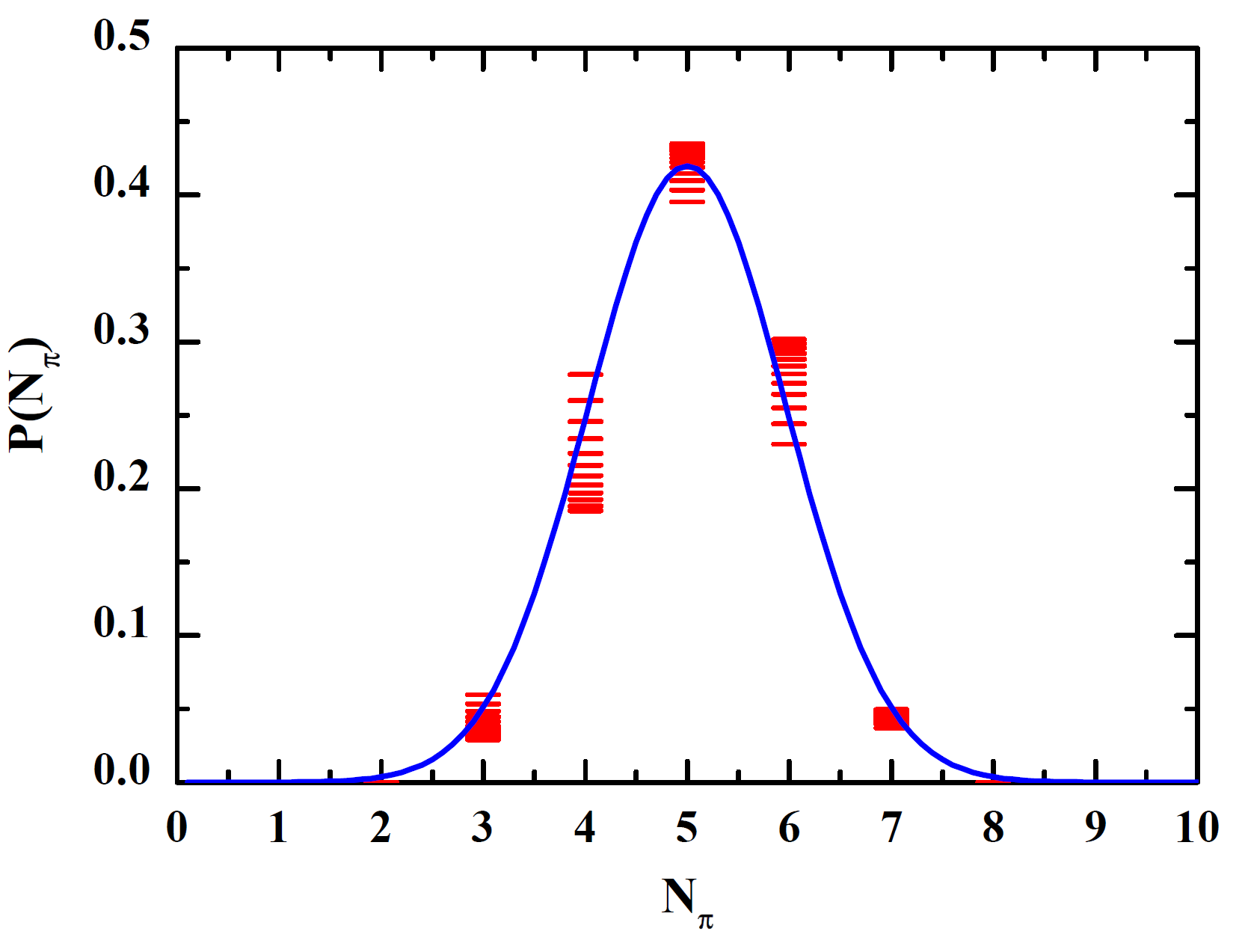
Figure 1: (Color online) Distribution in the final number of pions $P(N_{\pi})$ for $p\bar{p}$ annihilation at invariant energies $2.3\,\mathrm{GeV}\leq\sqrt{s}\leq 4\,\mathrm{GeV}$ from the QRP (short lines). The solid line is a gaussian parametrization fitted to the experimental data. The figure is taken from Ref. Cassing:2001ds .

III Quark rearrangement model for $B+\bar{B}$ production and annihilation

In this section we present the quark rearrangement model and the most relevant equations for the two- and three-body scattering rates. An extensive description for the invariant reaction rates for general particle number changing processes as well as the motivation for the quark rearrangement model is given in Ref. Cassing:2001ds .

III.1 Concept

As discussed in Ref. Cassing:2001ds one experimentally finds a dominant annihilation of $p\bar{p}$ into 5 pions at invariant energies $2.3\,\mathrm{GeV}\leq\sqrt{s}\leq 4\,\mathrm{GeV}$, see Fig. 1.

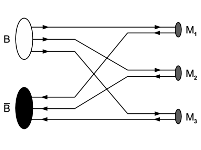
Figure 2: Illustration of the quark rearrangement model for a general baryon antibaryon pair $B\bar{B}$ annihilating into three mesons $M$ and vice versa. Here the meson $M_{i}$ may be any of the $0^{-}$ or $1^{-}$ nonets.

The final number of 5 pions may be interpreted as an initial annihilation into $\pi\rho\rho$ with the $\rho$ mesons decaying subsequently into two pions each. The channel $\pi\pi\rho$ then leads to 4 final pions, the channel $\pi\omega\rho$ to 6 final pions, the channel $\rho\omega\rho$ to 7 final pions etc. Accordingly, the baryon-antibaryon annihilation in the first step is a two-to-three reaction with a conserved number of quarks and antiquarks. This is the basic assumption of the quark rearrangement model which is also illustrated in Fig. 2. The annihilation reaction $p\bar{p}\rightarrow\pi\rho\rho$ is the dominant process in $p\bar{p}$ annihilation for invariant masses below 4 GeV, typical for the hadronic phase of a heavy-ion collision. By allowing the mesons $M_{i}$ to be any member of the $0^{-}$ or $1^{-}$ nonets one can describe an arbitrary $B\bar{B}$ annihilation and recreation by rearranging the quark and antiquark content. An implementation of baryon-antibaryon annihilation in such a manner misses the annihilation into one or two mesons, however, higher numbers of final mesons are implemented through the subsequent decay channels. This approach gives a realistic description for $p{\bar{p}}$ annihilation and we assume that for other baryon-antibaryon pairs than $p\bar{p}$ a similar annihilation pattern holds. Since there are no measurements of annihilation cross sections other than $p\bar{n}$ and $p\bar{p}$ this is our best guess which might be falsified by experiment.

III.2 Covariant transition rates

The quark rearrangement model only contains reactions of the kind $2\leftrightarrow 3$. The detailed balance based Lorentz invariant on-shell collision rate for the reaction $B\bar{B}\rightarrow 3M$ in a volume element of size d$V$ and time-step size d$t$ is written as Cassing:2001ds :

$$\frac{\mathrm{d}N_{\mathrm{coll}}[B\bar{B}\rightarrow 3\leavevmode\nobreak\ \mathrm{mesons}]}{\mathrm{d}t\,\mathrm{d}V}=\\ \sum_{c}\sum_{c^{\prime}}\frac{1}{(2\pi)^{6}}\int\frac{\mathrm{d}^{3}p_{1}}{2E_{1}}\frac{\mathrm{d}^{3}p_{2}}{2E_{2}}\leavevmode\nobreak\ W_{2,3}(\sqrt{s})\\ \times R_{3}(p_{1}+p_{2};c)N_{\mathrm{fin}}^{c}f_{1}(x,p_{1})f_{2}(x,p_{2}).$$ (1)

In (1) $c^{\prime}$ denotes all $B\bar{B}$ pairs with the properties $c^{\prime}=(m_{1}^{c^{\prime}},m_{2}^{c^{\prime}};\nu^{c^{\prime}})$; $c$ are all the possible meson channels with $c=(m_{3}^{c},m_{4}^{c},m_{5}^{c};\lambda^{c})$, with $m$ being the masses of the respective particles, and $\nu$ and $\lambda$ the quantum numbers signifying the channel (charge, parity, spin and strangeness). We assume that the transition matrix element squared $W_{2,3}$ does not significantly depend on the outgoing momenta and just on the invariant mass of the reaction, which holds approximately true for $p\bar{p}$ as we will see later. A formulation based on the matrix element will ensure detailed balance. The on-shell $n$-body phase-space integral is defined by

$$\begin{split}R_{n}(P;m_{1},\ldots,m_{n})=\left(\frac{1}{(2\pi)^{3}}\right)^{n}&\int\prod_{k=1}^{n}\frac{\mathrm{d}^{3}p_{k}}{2E_{k}}\leavevmode\nobreak\ (2\pi)^{4}\\ &\times\delta^{4}\left(P-\sum_{j=1}^{n}p_{j}\right)\end{split}$$ (2)

and in case of a constant transition matrix element dominates the interaction rate of the system. The factor $N_{\mathrm{fin}}^{c}$ is the multiplicity of the meson triple $c$ and results from the summation over the spin $s$ and possible isospin projections $F_{\mathrm{iso}}$ compatible with charge conservation of the meson channel $c$:

$$N_{\mathrm{fin}}^{c}=(2s_{3}+1)(2s_{4}+1)(2s_{5}+1)\frac{F_{\mathrm{iso}}}{N_{\mathrm{id}}!}.$$ (3)

The division by $N_{\mathrm{id}}!$, with $N_{\mathrm{id}}$ denoting the number of identical mesons, ensures that each charge configuration is only considered once for a given meson triple. The functions $f$ are the distribution functions of the $B\bar{B}$ pair in momentum and coordinate space. When looking at a specific $B\bar{B}$ pair one has to make sure that only meson channels are considered which conserve charge, energy and parity. The probability of this specific $B\bar{B}$ pair $c^{\prime}$ to annihilate into any of these possible meson channels $c$ is related to the total annihilation cross section of the $B\bar{B}$-pair $\sigma_{\mathrm{ann}}^{c^{\prime}}$ kajantie :

$$\begin{split}\frac{P^{c^{\prime}}_{\mathrm{tot}}\mathrm{d}V}{\mathrm{d}t}=&\frac{1}{4E_{1}E_{2}}\sum_{c}W_{2,3}(\sqrt{s})R_{3}(p_{1}+p_{2};c)N_{\mathrm{fin}}^{c}\\ =&v_{\mathrm{rel}}\sigma^{c^{\prime}}_{\mathrm{ann}}(\sqrt{s}),\end{split}$$ (4)

$$v_{\mathrm{rel}}=\frac{\sqrt{\lambda(s,m_{1}^{2},m_{2}^{2})}}{2E_{1}E_{2}}\leavevmode\nobreak\ ;\leavevmode\nobreak\ \lambda(a,b,c)=(a-b-c)^{2}-4bc,$$ (5)

where $dV$ and $dt$ are taken finite. The probability for a specific final state $\tilde{P}^{c^{\prime}\rightarrow c}$ in case of an annihilation is then given by the available phase space and the multiplicity of all possible meson channels $c$:

$$\tilde{P}^{c^{\prime}\rightarrow c}=N_{3}(c,c^{\prime},\sqrt{s})R_{3}(p_{1}+p_{2};c)N_{\mathrm{fin}}^{c},$$ (6)

$$\mathrm{with}\quad N_{3}^{-1}(c,c^{\prime},\sqrt{s})=\sum_{c}R_{3}(p_{1}+p_{2};c)N_{\mathrm{fin}}^{c}.$$ (7)

In a similar manner one finds for the probability of a specific meson channel $c$ fusing together and forming a specific $B\bar{B}$ pair $c^{\prime}$,

$$\begin{split}\frac{P^{c\rightarrow c^{\prime}}\mathrm{d}V^{2}}{\mathrm{d}t}=&\frac{1}{4E_{3}E_{4}E_{5}}\sigma_{\mathrm{ann}}^{c^{\prime}}(\sqrt{s})N_{3}(c,c^{\prime},\sqrt{s})\\ &\times\frac{\lambda(s,m_{1}^{2},m_{2}^{2})}{8\pi s}N_{B}^{c^{\prime}},\end{split}$$ (8)

with $N_{B}^{c^{\prime}}=(2s_{1}+1)(2s_{2}+1)$ denoting the multiplicity of the $B\bar{B}$ pair. A more detailed derivation of these formulae is given in Appendix A.

III.3 Annihilation cross sections

For the calculation of actual collision probabilities, Eq. (4) and (8), we are still missing the cross sections. As already mentioned above we assume the cross sections to depend only on the invariant energy, not the outgoing momenta. This assumption is approximately fulfilled for $p\bar{p}$ and $p\bar{n}$ annihilation, see Fig. 3. Other channels have not been measured so far. Since there are no experimental data available we assume a similar behavior for different spin combinations like $p\bar{\Delta}$.

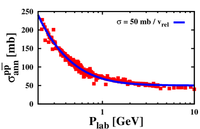
Figure 3: (Color online) $p\bar{p}$ annihilation cross section as a function of momentum in the laboratory $P_{lab}$. The data points are taken from Agashe:2014kda and the solid line is a fit by the function 50 mb/$v_{\mathrm{rel}}$ with $v_{\mathrm{rel}}$ denoting the relative velocity in the laboratory system (5).

In this work we investigate in particular the strangeness sector. We model the cross sections of particles with strangeness by

$$\sigma^{c^{\prime}}_{\mathrm{ann}}(\sqrt{s})=\sigma^{p\bar{p}}_{\mathrm{ann}}\lambda^{\varsigma+\bar{\varsigma}},$$ (9)

where $\varsigma$ and $\bar{\varsigma}$ are the number of strange and antistrange quarks in the $B\bar{B}$ pair $c^{\prime}$ and $\lambda\in[0,1]$ is a factor suppressing the transition matrix element for particles taking part in the quark rearrangement model and effectively suppressing the cross section. This parametrization is motivated by PYTHIA PYTHIA simulations where one sees a similar suppression for particles with strangeness compared to non-strange particles at the same energy above threshold. In the final implementation in PHSD the suppression factor has the value $\lambda$=0.5 which is in rough agreement with the PYTHIA simulations embedded in PHSD. We choose a dependence on not just the net strangeness $S$ but the sum of strange and antistrange quarks $\bar{\varsigma}+\varsigma$ due to their higher mass and a subsequent suppression of the rearrangement. The implementation with the strangeness $|S|=|\bar{\varsigma}-\varsigma|$ instead of $\bar{\varsigma}+\varsigma$ has no practical influence on the final results in case of relativistic heavy-ion collisions (cf. Appendix E).

IV Simulations in a finite box

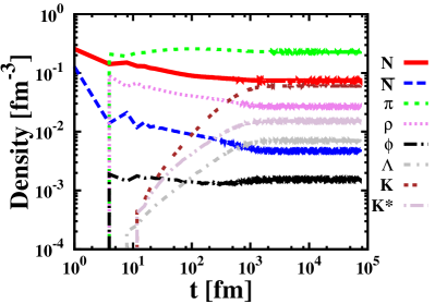
Figure 4: (Color online) Particle densities of a $p\bar{p}$ initialized system as a function of time. The particle species correspond to the following lines: the red solid line corresponds to nucleons, the blue dashed line to antinucleons, the green short-dashed line to pions, the violet dotted line to $\rho$ mesons, the black dashed-dotted line to $\phi$ mesons, the grey dashed-doubly-dotted line to $\Lambda$s, the brown doubly-dashed line to kaons and the beige short-dashed-dotted line to the vector kaons $K^{*}$. The different charge states of the particles have been summed over and $K$ denotes the sum of $K^{+},\leavevmode\nobreak\ K^{-},\leavevmode\nobreak\ K^{0}$ and $\bar{K}^{0}$.

This section addresses the implementation of the $2\leftrightarrow 3$ reactions formulated above in PHSD and checks the consistency of the numerical implementation. We use transport simulations in a box with periodic boundary conditions to investigate the behavior of the quark rearrangement model in equilibrium. We recall that in equilibrium - according to detailed balance - the reaction rate for $B\bar{B}\rightarrow 3M$ should be the same as for $3M\rightarrow B\bar{B}$. Furthermore, for a consistent implementation detailed balance should not only be fulfilled for the sum of all reaction channels but on a channel by channel basis. In the box simulations only the $B\bar{B}\leftrightarrow 3M$ reactions are considered now and all particles are taken as stable such that no decays occur. The particles incorporated are the $0^{-},1^{-}$ meson nonets, the $1/2^{+}$ baryon octet and the $3/2^{+}$ baryon decuplet. Additionally, we consider N(1440) and N(1535) baryonic resonances. Furthermore, we take into account the strangeness content of $\eta$ and $\phi$ with 50% and 83.1% $s\bar{s}$ content, respectively. With this the number of possible mass channels amounts to more than 2000. Hence, an initialization with every possible channel is not feasible. Therefore, we look at systems which are initialized by a single type of baryon and antibaryon adding up to 100 systems for the consistency check. The box simulations have the following initial conditions:

• Box volume lies around 18000 fm³ with periodic boundary conditions

• All simulations have the same energy density $\epsilon=0.4$ GeV/fm³ with 10% of the energy distributed to kinetic energy

• The ratio between baryons and antibaryons is set to 2:1 and the net baryon density amounts to $\rho_{B}\approx 0.2$ fm^-3

• The initial momentum distribution is of Boltzmann-shape

• For the box simulations a suppression of channels including strangeness is neglected.

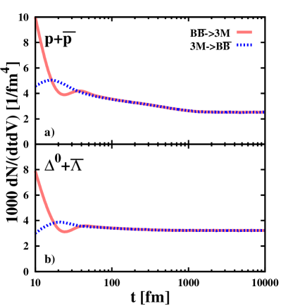
Figure 5: (Color online) Total reaction rate (per volume $dV$) as a function of time for two different initializations. The solid (slightly transparent) red lines correspond to the baryon-antibaryon annihilation and the red dotted lines to the formation. The systems are initialized in a) with only $p+\bar{p}$ and in b) with only $\Delta^{0}+\bar{\Lambda}$.

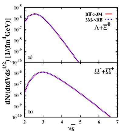
Figure 6: (Color online) Total reaction rate as a function of the invariant mass $\sqrt{s}$ in equilibrium for five different initializations. The solid (slightly transparent) red line corresponds to the baryon-antibaryon annihilation and the red dotted line to the formation. The systems are initialized in a) with only $\Lambda+\bar{\Xi}^{0}$ and in b) with only $\Omega^{-}+\bar{\Omega}^{+}$.

Before the actual calculations the three-body phase-space integrals $R_{3}$ have been calculated and fitted by proper functionals to save enormous CPU time. In detail, the three-body phase-space integrals $R_{3}$, depending on invariant energy and three masses $m_{i}$,

$$R_{3}(\sqrt{s};m_{1},m_{2},m_{3})=\\ \int\limits_{(m_{1}+m_{2})^{2}}^{(\sqrt{s}-m_{3})^{2}}\frac{\mathrm{d}M_{2}^{2}}{2\pi}R_{2}(\sqrt{s};m_{3},M_{2})R_{2}(M_{2};m_{1},m_{2}),$$ (10)

with $R_{2}$ defined in Eq. (25) are fitted by

$$R_{3}(t,m_{1},m_{2},m_{3})=a_{1}t^{a_{2}}\left(1-\frac{1}{a_{3}t+1+a_{4}}\right),$$ (11)

with $t=\sqrt{s}-m_{1}-m_{2}-m_{3}$ and $a_{i}>0$. The fit parameters $a_{i}$ have been evaluated for each combination of meson masses $m_{1},m_{2},m_{3}$ and stored on file. For further details on the phase-space integrals we refer the reader to appendix B.

We recall that the fusion of three mesons can not be described in a Lorentz invariant way by geometrical collision criteria between the particles due to the three inertial systems. To find a solution we employ the in-cell method introduced by Lang et al. in-cell-method and adopted in Ref. Cassing:2001ds . This method is also employed for $2\leftrightarrow 3$ reactions in partonic cascade calculations Greiner . The in-cell method can be used for any number of colliding particles since there is no problem with time ordering due to the locality of the formulation. In the in-cell method space-time is divided into four dimensional cells with widths $\Delta x,\Delta y,\Delta z,\Delta t$ and only particles inside the same cell may collide with each other. One calculates the reaction probabilities of each particle with every other one inside the same cell. The actual collision and the final state is chosen via Monte-Carlo. The possible final states and multiplicities in Eqs. (4) and (8) are precalculated to save computational time during the transport simulation. The cell size and the time step $\Delta t$ are optimized for the problem under investigation such that the total probability of a transition in a local cell does not exceed unity but is also not too small. For the actual calculations shown below we use $dt$ = 4 fm/c and $dV$=40 fm³ which ensures that the transition probabilities are always below unity.

Table 1: Deviation from detailed balance $\delta$ (12) for selected systems and as the average over all 100 investigated systems $\langle\delta\rangle$.

rank	$p+\bar{p}$		$\Delta^{0}+\bar{\Lambda}$		$\Lambda+\bar{\Xi}^{0}$		$\langle\delta\rangle$ [%]
	channel	$\delta$ [%]	channel	$\delta$ [%]	channel	$\delta$ [%]
1	$N\bar{N}\leftrightarrow\pi\pi\rho$	0.17	$N\bar{\Xi}\leftrightarrow\pi KK^{*}$	1.45	$N\bar{N}\leftrightarrow\pi\pi\rho$	0.13	1.24
2	$N\bar{N}\leftrightarrow\pi\rho\rho$	3.06	$N\bar{\Omega}\leftrightarrow KK^{*}K^{*}$	3.59	$N\bar{\Delta}\leftrightarrow\pi\rho\rho$	1.70	1.82
3	$N\bar{\Delta}\leftrightarrow\pi\pi\rho$	1.58	$\Delta\bar{\Xi}\leftrightarrow\pi KK^{*}$	1.32	$N\bar{\Delta}\leftrightarrow\pi\pi\rho$	2.04	1.70
4	$N\bar{\Delta}\leftrightarrow\pi\rho\rho$	0.84	$\Delta\bar{\Xi}\leftrightarrow KK^{*}\rho$	0.64	$N\bar{N}\leftrightarrow\pi\rho\rho$	3.31	1.54
5	$\Delta\bar{N}\leftrightarrow\pi\pi\rho$	2.43	$\Delta\bar{\Omega}\leftrightarrow KK^{*}K^{*}$	1.08	$\Delta\bar{N}\leftrightarrow\pi\rho\rho$	1.33	1.49
6	$\Delta\bar{N}\leftrightarrow\pi\rho\rho$	0.73	$N\bar{\Sigma}\leftrightarrow\pi K^{*}\rho$	3.58	$\Delta\bar{N}\leftrightarrow\pi\pi\rho$	2.71	1.97
7	$N\bar{N}\leftrightarrow\pi\pi a_{1}$	6.52	$\Delta\bar{\Sigma}\leftrightarrow\pi K^{*}\rho$	2.00	$\Delta\bar{\Delta}\leftrightarrow\pi\pi\rho$	2.69	2.04
8	$N\bar{N}\leftrightarrow\pi\pi\pi$	5.10	$N\bar{N}\leftrightarrow\pi\pi\rho$	0.23	$N\bar{\Sigma}\leftrightarrow\pi K^{*}\rho$	2.04	2.03
9	$N\bar{\Sigma}\leftrightarrow\pi K\rho$	0.31	$N\bar{\Sigma}\leftrightarrow\pi K\rho$	0.42	$\Delta\bar{\Delta}\leftrightarrow\pi\pi\rho$	2.12	2.11
10	$N\bar{\Sigma}\leftrightarrow\pi K^{*}\rho$	0.96	$N\bar{\Omega}\leftrightarrow KKK$	0.35	$N\bar{\Sigma}\leftrightarrow\pi K\rho$	0.35	2.11

We now discuss results for a few selected systems. We present randomly picked ensembles that cover the qualitative range of possible systems, i.e. systems consisting of only initial light quarks, only initial strange/antistrange quarks as well as a variety of combinations of light and strange quarks/antiquarks. In Fig. 4 the time evolution of the particle densities for a system initialized with protons and antiprotons is shown to demonstrate the production and annihilation of different particle species in a system consisting initially only of protons and antiprotons. After the first timestep of the simulation a lot of new mesons like pions, $\rho$ and $\omega$ mesons are formed. At later times also strange mesons and baryons are formed because of the partial $s\bar{s}$ content of $\phi$ and $\eta$. In equilibrium the system has a significant amount of mesons and baryons with strange and antistrange quarks. However, the generation of strange quarks even for the meson sector takes a long time ($\approx$ 60 fm/c) to produce significantly high strange particle densities; thus the generation via $\phi$ and $\eta$ should have negligible influence on actual heavy-ion collisions since large densities are needed for a significant contribution from the meson fusion. In a 5% central Pb+Pb collision at 158$A$ GeV the meson fusion dies out at $\sim$ 13 fm/c which is insufficient for having a major influence on the strangeness sector, see Fig. 7 (discussed in section V below).

We show in Fig. 5 the total reaction rate as a function of time for two exemplary initializations which were initialized with $p+\bar{p}$ and $\Delta^{0}+\bar{\Lambda}$, respectively. Both systems share a similar evolution of the total reaction rate. All systems reach detailed balance much faster ($\approx$ 40 fm) than they reach equilibrium ($\approx$ 1000 fm).

Detailed balance should also be valid for the total reaction rate as function of the invariant mass. For this we show in Fig. 6 the total reaction rate as a function of the invariant mass $\sqrt{s}$ in the plateau region of Fig. 5 which is associated with the equilibrium state. From Fig. 6 we see that detailed balance is also fulfilled for this quantity. Note that the maximum achievable invariant mass of particles participating in annihaltion or recreation (in equilibrium) is lower in systems initialized with lighter baryons than for systems initialized with heavier ones.

The last most crucial check for detailed balance is the fulfilment on a channel by channel basis. To this end we define the deviation from detailed balance for each channel by

$$\delta=1-\frac{\frac{\mathrm{d}N}{\mathrm{d}t}(B\bar{B}\rightarrow 3M)}{\frac{\mathrm{d}N}{\mathrm{d}t}(3M\rightarrow B\bar{B})}.$$ (12)

We calculate $\delta$ for each of the more than 2000 channels and look at the channels with the largest reaction rates in all 100 investigated systems. In Tab. 1 the 10 most important channels with the largest reaction rates are shown from highest to lowest for 3 of the exemplary systems as well as the average for all 100 investigated systems and the average over all channels. The average over all 100 investigated systems shows that detailed balance is fulfilled better than 97% on a channel-by-channel basis for the 100 most dominant channels. This verifies the correct implementation of the baryon-antibaryon annihilation and recreation within the quark rearrangement model in the PHSD transport approach. Some channels of a system may deviate by more than 5% from detailed balance, however, this is a relict of too low statistics. We found only few channels ($\approx$ 20 for the 10 most dominant channels) that had a deviation of up to 9%. In general these deviations may be neglected as can be seen in the averaged values and the dominant number of channels being very close to detailed balance which gives a proof for the working principle of the implementation presented.

V PHSD simulations for heavy-ion collisions

In this section we show the influence of the additional channels in the strangeness sector for $B\bar{B}\leftrightarrow 3M$ reactions on heavy-ion collisions in the energy regime of 11.7-158$A$ GeV.

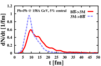
Figure 7: (Color online) The reaction rate of the $B\bar{B}\leftrightarrow 3M$ reactions (solid line) as a function of time in 5% central Pb+Pb collisions at 158$A$ GeV in comparison to the total three-meson fusion rate (dashed line).

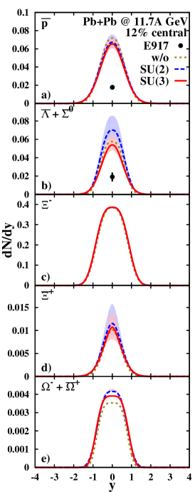
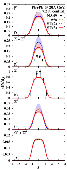
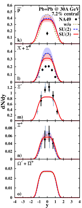
Figure 8: (Color online) Rapidity spectra of ${\bar{p}},{\bar{\Lambda}}+{\bar{\Sigma}}^{0},\Xi^{-},{\bar{\Xi}}^{+},\Omega^{-}+{\bar{\Omega}}^{+}$ in (12%) 7.2% central Pb+Pb collisions at 11.7, 20 and 30$A$ GeV. The solid lines show the results when including all light and strange quark channels (denoted by SU(3)) while the dashed lines results from discarding strange or antistrange quarks in the reaction channels (denoted by SU(2)). The error bands indicate the systematic uncertainty of the calculations due to a different ensemble size. The dotted lines show the results with $B\bar{B}\leftrightarrow 3M$ reactions switched off. The data points are taken from Refs. Back:2001ai ; Anticic:2010mp ; Alt:2008qm .

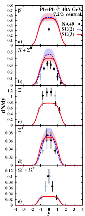
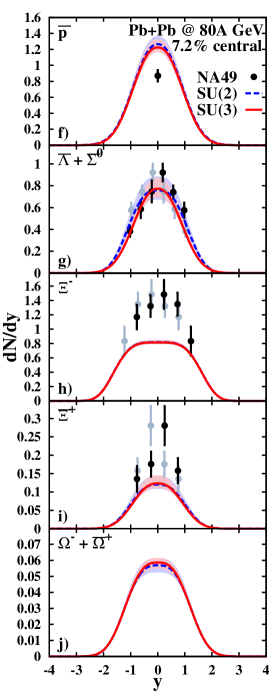
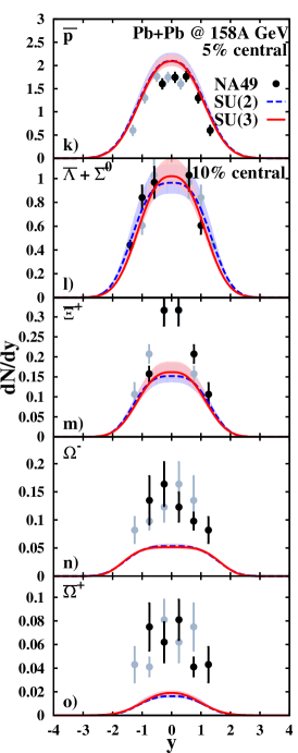
Figure 9: (Color online) Rapidity spectra ${\bar{p}},{\bar{\Lambda}}+{\bar{\Sigma}}^{0},\Xi^{-},{\bar{\Xi}}^{+},\Omega^{-}+{\bar{\Omega}}^{+}$ in central Pb+Pb collisions at 40, 80 and 158$A$ GeV for $B\bar{B}\leftrightarrow 3M$ with only light quarks (dashed lines) and including strange quarks (solid lines) compared to experimental measurements. The error bands indicate the systematic uncertainty of the calculations due to a different ensemble size. The data points are taken from Refs. Anticic:2010mp ; Alt:2008qm ; Alt:2004kq ; Alt:2006dk .

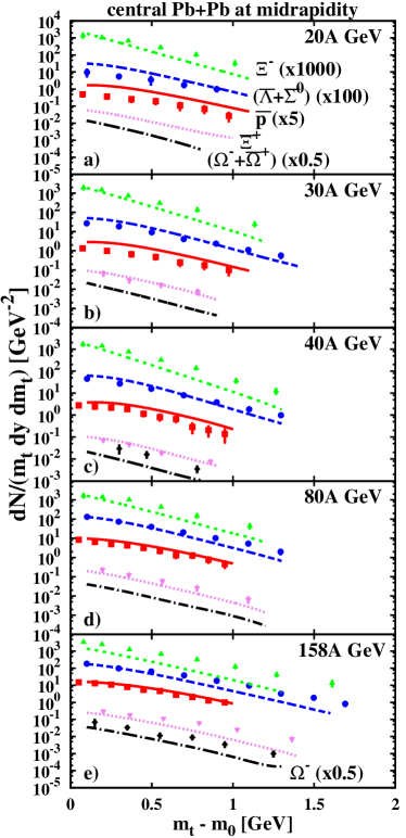
Figure 10: (Color online) Transverse mass spectra for central Pb+Pb collisions at midrapidity. The centrality selection for the particles at the different energies is the same as in Figs. 8 and 9. The particles in each panel are from top to bottom $\Xi^{-},\bar{\Lambda}+\bar{\Sigma}^{0},\bar{p},\bar{\Xi}^{+}$ and $\Omega^{-}+\bar{\Omega}^{+}$, only at 158$A$ GeV the lowest lying line corresponds to $\Omega^{-}$. The data points are taken from Refs. Alt:2008qm ; Alt:2004kq ; Alt:2006dk .

Before coming to the actual results we compare in Fig. 7 the reaction rate for the total baryon-antibaryon annihilation (solid line) and formation (dashed line) from PHSD in 5% central Pb+Pb collisions at 158$A$ GeV. Whereas the meson-fusion rate dominates at early times ($<$ 13 fm/c) the annihilation takes over for larger times during the final expansion of the system. Although the time integrals of both rates are about the same there is no appreciable time interval in which both rates are identical. This indicates a strong nonequilibrium dynamics of baryon-antibaryon annihilation and reproduction in actual heavy-ion reactions.

We note that a similar analysis has been performed in the earlier study in Ref. Cassing:2001ds (Fig. 7) on the basis of the HSD transport model (version 2.3) for the same system, however, without averaging over the ensembles. The earlier rates differ substantially from the present results from PHSD (version 4.0) due to the different degrees of freedom in the initial phase of the collision. In order to quantify the differences we have recalculated the rates within HSD2.3 (from the year 2002) and compared the numbers with those from PHSD4.0, which is the most recent version including also the effects from chiral symmetry restoration AlesPaper (PHSD3.3) and nonperturbative charm dynamics as well as extended $2\leftrightarrow 3$ reactions. We found that both rates (from HSD2.3 and PHSD4.0) differ only slightly for times $\geq$ 6 fm/c (after contact of Pb+Pb at b=2fm) but the huge rates (from HSD2.3) at the first few fm/c are essentially missing in PHSD4.0. This is due to the fact that at the top SPS energy the initial energy conversion goes to interacting partons in PHSD4.0 and not to strings decaying to hadrons (and partly to $B{\bar{B}}$ pairs) in HSD2.3. Thus in PHSD4.0 (at the top SPS energy) there are initially no $B{\bar{B}}$ pairs that might annihilate nor mesons that might fuse! Due to the very high hadron densities in HSD2.3 (after string decay) both the annihilation and reproduction rates are very high and about equal whereas in the hadronic expansion phase the densities are sizeably lower. In this dilute regime the 3-body channels first dominate and decrease fast in time whereas the 2-body annihilation reactions still continue for some time. As addressed in the Introduction we thus expect also differences in the antibaryon rapidity spectra as compared to the early results from HSD2.3 Cassing:2001ds . However, in both transport calculations – incorporating the $2\leftrightarrow 3$ reactions – the time integrated rates for annihilation and reproduction turn out to be about equal.

The actual PHSD calculations for relativistic nucleus-nucleus collisions are carried out in the parallel ensemble method, i.e. in case of the cascade mode a typical number of 100 - 300 ensembles are propagated in time fully independent from each other. However, the calculation of net-baryon densities, scalar densities and energy densities - needed for the full PHSD dynamics - is carried out by averaging over all ensembles. This results in a crosstalk between ensembles due to the propagation of particles in the self-generated mean fields (for partons and baryons/antibaryons) as well as in the baryon/antibaryon formation in the hadronization. A systematic study of all particle spectra in rapidity and transverse mass shows that the results for mesons and baryons well scale with the number of ensembles whereas the antibaryon sector shows small variations with the number of ensembles. This scaling violation is essentially due to the numerical approximations that have to be presently introduced in order to keep the huge number of reaction channels manageable. This introduces a systematic error in our calculations for the antibaryon sector which is accounted for by hatched bands in the following figures. The solid or dashed lines correspond to the standard ensemble number of 150 used as default in PHSD calculations in the energy range of interest.

V.1 Rapidity and transverse mass spectra

We now discuss the influence of the $B{\bar{B}}\leftrightarrow 3M$ reactions on observables measured in actual experiments from 11.7 - 158$A$ GeV. We first focus on rapidity spectra and mention that the $B\bar{B}\leftrightarrow 3M$ reactions have practically no influence on baryon and meson spectra AlesPaper and, hence, we only show the results for the relevant antibaryons and $\Xi^{-}$ to demonstrate that the influence on baryons is barely visible. For results on meson and baryon spectra we refer the reader to the review review and Ref. AlesPaper . As mentioned above the full, dashed and dotted lines show the results for 150 ensembles; the blue and red hatched areas result when employing different ensemble numbers in a wide range.

We first focus on the influence of the newly incorporated strangeness sector. In the following, we compare the implementation with only light quark channels (SU(2)) with the new one including also the strangeness sector (SU(3)). The rapidity spectra of ${\bar{p}},{\bar{\Lambda}}+{\bar{\Sigma}}^{0},\Xi^{-},{\bar{\Xi}}^{+},\Omega^{-}+{\bar{\Omega}}^{+}$ for central Pb+Pb collisions from 11.7 to 158$A$ GeV are shown in Figs. 8 and 9. The rapidity spectra of the anti-hyperons are overall closer to the experimental data when taking into account the strangeness sector for the $B\bar{B}\leftrightarrow 3M$ reactions. However, the antiproton spectra are faintly influenced by the incorporated sector and describe the data only moderately well. In general the investigations suggest that the $B\bar{B}\leftrightarrow 3M$ reactions have the largest impact at energies below 80$A$ GeV. This result shows that the consideration of the strange quarks helps improving the description of a heavy-ion collision in the framework of PHSD. For particles like $\bar{\Xi}^{+},\Omega^{-}$ and $\bar{\Omega}^{-}$ at lower energies, where currently no experimental data are available, our results should be taken as predictions.

In Fig. 8 we, furthermore, show results from calculations neglecting the $B\bar{B}\leftrightarrow 3M$ reactions. We find that the rapidity distribution for $\bar{p}$ has a higher peak and is narrower compared to calculations with $B\bar{B}\leftrightarrow 3M$, while the total number of antiprotons is about the same. The results for the antihyperons - starting from 20$A$ GeV - lie on top of the SU(2) simulations. At 11.7$A$ GeV the hyperon spectra are closer to the SU(3) calculations and for $\Omega^{-}+\bar{\Omega}^{+}$ lie even below those.

Another interesting observable measured in experiment is the transverse mass ($m_{t}$) spectrum at midrapidity, i.e. $dN/(m_{t}dydm_{t})$ as displayed in Fig. 10. Here the additional strangeness sector has qualitatively the same impact as for the rapidity spectra. Accordingly, we only show results for central Pb+Pb collisions in the energy regime from 20 to 158$A$ GeV including the strangeness sector for the $B\bar{B}\leftrightarrow 3M$ reactions. For the $\Xi^{-}$ we find that PHSD describes the low $m_{t}$ regime for energies below 158$A$ GeV rather well. However, for higher $m_{t}$ the data points are missed due to a harder experimental slope of the spectrum. At 158$A$ GeV some $\Xi^{-}$’s are missed in the low $m_{t}$ regime. The $\bar{\Lambda}+\bar{\Sigma}^{0}$ spectrum is close to the experimentally measured data for all energies, however, at 158$A$ GeV it falls off too fast. The transverse mass spectra of the antiprotons are overall in very good agreement with experiment, the only drawback is the overproduction at midrapidity which is most visible for 20 and 30$A$ GeV. Also, the $\bar{\Xi}^{+}$ are in close vicinity to the experimental data for energies smaller than 158$A$ GeV, but fall off too quickly at 158$A$ GeV. The production of $\Omega^{-}$ and $\bar{\Omega}^{+}$ was underestimated already in the rapidity spectra, see Fig. 9, but looking at the transverse mass spectra at 158$A$ GeV the results are in reasonable agreement with experiment for $m_{t}<0.8$ GeV.

V.2 Impact of chiral symmetry restoration and deconfinement

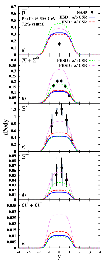
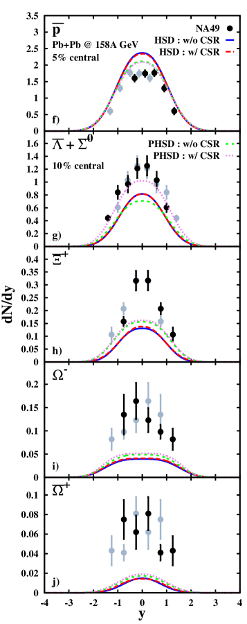
Figure 11: (Color online) Rapidity spectra for a central Pb+Pb collision at 30 and 158$A$ GeV; comparison between simulations with (PHSD) and without (HSD) the deconfinement transition and with activated and deactivated chiral symmetry restoration (CSR). The data points are taken from Refs. Anticic:2010mp ; Alt:2008qm ; Alt:2004kq ; Alt:2006dk .

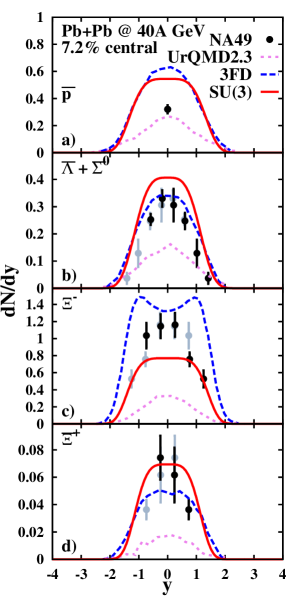
Figure 12: (Color online) Rapidity spectra for a central Pb+Pb collision at 40$A$ GeV; comparison between PHSD results with the $B\bar{B}\leftrightarrow 3M$ reactions including strangeness (red solid line), UrQMD-2.3 Petersen:2008kb (violet short-dashed line) and 3FD with a 2-phase equation of state Ivanov:2013yqa (blue dashed line). The experimental data are taken from Refs. Anticic:2010mp ; Alt:2008qm .

We now address the question with respect to traces of chiral symmetry restoration and deconfinement in the antibaryon and multi-strange baryon spectra from central Pb+Pb collisions at SPS energies. We recall that clear signals have been found before in the strange meson and baryon rapidity distributions Cass16 ; AlesPaper and one might speculate if a similar signal can be seen in the antibaryon sector. To this aim we perform transport calculations - including the $B{\bar{B}}\leftrightarrow 3M$ channels specified above - with different settings:

• HSD calculations without chiral symmetry restoration (CSR) and deconfinement since HSD does not include a partonic phase

• HSD calculations with chiral symmetry restoration (CSR) in the hadronic phase but without deconfinement

• PHSD calculations without chiral symmetry restoration (CSR) in the hadronic phase but with a deconfinement transition

• PHSD calculations with chiral symmetry restoration (CSR) in the hadronic phase and with a deconfinement transition.

The systems addressed are central Pb+Pb collisions at 30 and 158$A$ GeV. The rapidity spectra for antibaryons and $\Xi^{-}$ are displayed in Fig. 11 and show that at 158$A$ GeV the impact of chiral symmetry restoration is very small in the HSD calculations (without deconfinement) as well as for PHSD (including deconfinement) except for the ${\bar{\Lambda}}+{\bar{\Sigma}}^{0}$ spectrum. When comparing HSD and PHSD results including CSR we find a slight reduction of the ${\bar{p}}$ spectra, a moderate enhancement for the ${\bar{\Lambda}}+{\bar{\Sigma}}^{0}$ spectrum and only a small enhancement for $\Xi^{\pm}$ and $\Omega^{-}+{\bar{\Omega}}^{+}$ when including a partonic phase. Since the reproduction of the multistrange sector by PHSD is very poor one cannot conclude on the presence of a deconfinement transition on the basis of the rapidity spectra shown in Fig. 11. Note, however, that a clear signal has been found in the elliptic and triangular flow before in Ref. Konchakovski:2012yg at this energy.

At 30$A$ GeV the situation is not much better. The PHSD calculations with CSR perform best for $\Xi^{-}$ and ${\bar{\Xi}}^{+}$, however, overestimate the ${\bar{p}}$ and ${\bar{\Lambda}}+{\bar{\Sigma}}^{0}$ yield. The HSD calculations are too low in the strange antibaryon sector including/excluding CSR providing some hint that a partonic phase should be present in a moderate space-time volume at this energy. Accordingly, the antibaryons and in particular the multi-strange sector do not give additional information on chiral symmetry restoration or deconfinement within the framework of PHSD calculations.

V.3 Comparison to other dynamical models

In this subsection we compare our current PHSD results to those from other dynamical models which have been employed for heavy-ion reactions in the SPS energy regime, in particular from the Ultra-relativistic Quantum Molecular Dynamics model (UrQMD) Bass:1998ca ; Bleicher:1999xi and the three-fluid dynamics model (3FD) 3FD . The UrQMD is a hadronic transport model including a multitude of hadronic resonances as well as strings that are responsible for multi-particle production. The 3FD is a fluid dynamical model describing - within the framework of hydrodynamics - the transition from the initial baryonic fluids (projectile and target) to the newly produced fluid (around midrapidity). For details we refer the reader to the original literature Bass:1998ca ; Bleicher:1999xi ; 3FD . We show in Fig. 12 our actual results in case of the rapidity spectra for a central Pb+Pb collision at 40$A$ GeV with the $B\bar{B}\leftrightarrow 3M$ reactions including the strangeness sector in comparison to results from the UrQMD Petersen:2008kb and the 3FD using a 2-phase equation of state Ivanov:2013yqa . The 3FD model, like PHSD, overshoots the antiproton yield whereas UrQMD is close to the experimental data. The $\bar{\Lambda}+\bar{\Sigma}^{0}$ spectrum is described by PHSD and the 3FD model similarly close to the experimental data whereas UrQMD produces too few. For the $\Xi^{-}$ all models show different behaviors; whereas the 3FD model overpredicts the production, PHSD produces slightly too few $\Xi^{-}$ at midrapidity but describes otherwise the shape well. UrQMD predicts (just like for $\bar{\Lambda}+\bar{\Sigma}^{0}$ and $\bar{\Xi}^{+}$) too few antibaryons since $B{\bar{B}}$ annihilation is incorporated, however, not the backward channels thus violating detailed balance. PHSD and the 3FD model are close to the experimental data for $\bar{\Xi}^{+}$, with the 3FD slightly underpredicting the yield. Depending on the particle species of interest one model describes some yield better than the other at higher SPS energies. In general, the 3FD model and PHSD appear to be similarly capable of roughly describing the dynamics of baryons and antibaryons with strangeness content in this energy range.

VI Summary

In this work we have recapitulated and extended the quark rearrangement model for baryon-antibaryon annihilation ($B{\bar{B}}\leftrightarrow 3M$) in the course of heavy-ion collisions. The approximate validity of this model was motivated by the distribution in the number of final state pions in $p\bar{p}$ annihilation for $2.3$ GeV$\leq\sqrt{s}\leq 4$ GeV (cf. Fig. 1), where the 3-body channel $\pi\rho\rho$ e.g. leads to 5 pions (on average) in the final state. Additionally to the HSD calculations in Ref. Cassing:2001ds , we have included in the $2\leftrightarrow 3$ channels the strangeness sector with a suppression factor for the matrix elements of particles having strange and anti-strange quarks. We have shown, using simulations in a box with periodic boundary conditions, that the numerical implementation of the quark rearrangement model including the strangeness sector satisfies the detailed balance $2\leftrightarrow 3$ relation on a channel-by-channel basis as well as differentially as a function of the invariant energy $\sqrt{s}$.

We found that the earlier rates from HSD2.3 Cassing:2001ds differ substantially from the present results from PHSD (version 4.0) due to the different degrees of freedom in the initial phase of the collision. Both rates (from HSD2.3 and PHSD4.0) differ only slightly for times $\geq$ 6 fm/c (after contact of Pb+Pb at b=2fm) but the huge rates (from HSD2.3) at the first few fm/c are essentially missing in PHSD4.0. This is due to the fact that at the top SPS energy the initial energy conversion goes to interacting partons in PHSD4.0 and not to strings decaying to hadrons (and partly to $B{\bar{B}}$ pairs) in HSD2.3. Thus in PHSD4.0 (at the top SPS and higher energies) there are initially no $B{\bar{B}}$ pairs that might annihilate nor mesons that might fuse! Due to the very high hadron densities in HSD2.3 (after string decay) both the annihilation and reproduction rates are very high and about equal whereas in the hadronic expansion phase the densities are sizeably lower. In this dilute regime the 3-body channels first dominate and decrease fast in time whereas the 2-body annihilation reactions still continue for some time. However, in both transport calculations – incorporating the $2\leftrightarrow 3$ reactions – the time integrated rates for annihilation and reproduction turn out to be about equal.

The influence of the newly implemented channels in the strangeness sector on actual heavy-ion collisions has been investigated in PHSD simulations (version 4.0) of central Pb+Pb collisions from 11.7-158$A$ GeV. The rapidity spectra of antibaryons - using the quark rearrangement model with and without the strangeness sector - have been compared to experimental data where available. Changes could only be seen for the antibaryons in the investigated energy regime whereas the meson and baryon sector are practically unchanged AlesPaper . Due to the chemical rearrangement between the baryons and mesons considered in $B\bar{B}\leftrightarrow 3M$ reactions an overall higher anti-proton production was observed for all energies which pushed the PHSD results up thus overestimating the experimental data. The other antibaryons got closer to the experimental data when the strangeness sector was included for the $B\bar{B}\leftrightarrow 3M$ reactions. For the energies investigated the strangeness sector has the largest impact at the lowest energies. The results show that the $B\bar{B}\leftrightarrow 3M$ reactions indeed need the strangeness sector to describe the heavy-ion collisions more properly. We note, however, that the quark rearrangement model might be too crude to allow for robust conclusions. We still need experimental information on baryon-antibaryon annihilation cross sections other than $p\bar{p}$ and $p\bar{n}$ to achieve a better description and understanding of heavy-ion collisions.

In addition to the rapidity spectra, we have shown the transverse mass spectra for various antibaryons and have seen that the low $m_{t}$ region is well described for all antibaryons with the exception of the antiprotons that are overpredicted at energies lower than 80$A$ GeV. For higher transverse masses some spectra fall off too fast thus underestimating the experimental data to some extent. Accordingly, our understanding of antibaryon dynamics is far from being complete and we might still miss essential ingredients.

We have additionally addressed the question if the antibaryon spectra (with strangeness) from central heavy-ion reactions at SPS energies provide further information on the issue of chiral symmetry restoration and deconfinement. By comparing results from HSD (without partonic phase) with those from PHSD (with partonic degrees of freedom) as well as including/excluding effects from chiral symmetry restoration (Fig. 11) we did not find convincing signals for either transition due to the strong final-state interactions.

Appendix A Meson fusion

In order to determine the probability for the three-meson fusion rate we start with the Lorentz-invariant reaction rate for this process Cassing:2001ds ,

$$\begin{split}&\frac{\mathrm{d}N_{\mathrm{coll}}[3\leavevmode\nobreak\ \mathrm{mesons}\rightarrow B\bar{B}]}{\mathrm{d}t\,\mathrm{d}V}=\\ &\sum_{c}\sum_{c^{\prime}}\frac{1}{(2\pi)^{9}}\int\frac{\mathrm{d}^{3}p_{3}}{2E_{3}}\frac{\mathrm{d}^{3}p_{4}}{2E_{4}}\frac{\mathrm{d}^{3}p_{5}}{2E_{5}}\leavevmode\nobreak\ W_{2,3}(\sqrt{s})\\ &\times R_{2}(p_{3}+p_{4}+p_{5};c^{\prime})N_{B}^{c^{\prime}}f_{3}(x,p_{3})f_{4}(x,p_{4})f_{5}(x,p_{5}),\end{split}$$ (13)

where $N_{B}^{c^{\prime}}$ denotes the multiplicity of the final state and the two-body phase-space integral $R_{2}$ is given by

$$R_{2}(\sqrt{s};m_{1},m_{2})=\frac{\sqrt{\lambda(s,m_{1}^{2},m_{2}^{2})}}{8\pi s}$$ (14)

with $\lambda$ defined in Eq. (5). The transition matrix element squared $W_{2,3}$ is not known but using Eq. (9) for our special problem of $2\leftrightarrow 3$ processes one gets,

$$\begin{split}\sum_{c}P_{c\rightarrow c^{\prime}}(\sqrt{s})=&\sum_{c}W_{2,3}(\sqrt{s})R_{3}(\sqrt{s},c)N_{\mathrm{fin}}^{c}\\ =&W_{2,3}N_{3}^{-1}(\sqrt{s},c^{\prime})\\ =&4E_{1}E_{2}v_{\mathrm{rel}}\sigma_{\mathrm{ann}}^{c^{\prime}}(\sqrt{s}),\end{split}$$ (15)

where we have taken $W_{2,3}$ out of the sum over the baryon-antibaryon pairs and end up with the expression for the normalisation constant for the invariant energy $\sqrt{s}$ from Eq. (7). Inserting Eq. (15) for the transition matrix element squared into (13) gives the result for the transition probability for the meson fusion in Eq. (8). Note that all energies and momenta in the calculations of the transition probabilities are in the lab frame.

Appendix B Phase-space integrals

The on-shell phase-space integrals occurring throughout this work inhibit most of the dynamics of the system. As they play a major role this section is dedicated to some more details of phase-space integrals. We recall that the $n$-body phase-space integral is generally defined by

$$R_{n}(P;m_{1},\ldots,m_{n})=\\ \left(\frac{1}{(2\pi)^{3}}\right)^{n}\int\prod_{k=1}^{n}\mathrm{d}^{4}p_{k}\leavevmode\nobreak\ \rho_{k}(p_{k})(2\pi)^{4}\delta^{4}\left(P-\sum_{j=1}^{n}p_{j}\right),$$ (16)

with $\rho$ denoting the spectral function of the respective particle. Since the phase-space integrals are Lorentz invariant we will always work in the center-of-mass system. In the on-shell case the spectral function takes the form

$$\rho(p)=\delta(p^{2}-m_{1}^{2})$$ (17)

with $p$ denoting the 4-momentum in this case. Inserting the spectral function (17) into Eq. (16) and integrating over $p^{0}$ yields the on-shell phase-space integral of Eq. (2). To show (as an example) the behavior of the different $n$-body phase-space integrals it is instructive to look e.g. at the consecutive decays $p\bar{p}\rightarrow\pi\rho\rho\rightarrow 3\pi\rho\rightarrow 5\pi$ which are essentially the motivation for the QRM. Also, this example connects the 3-,4- and 5-body phase-space integrals as a function of the invariant energy above threshold (see below).

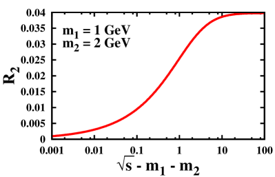
Figure 13: Two-body phase-space integral for particles with masses $m_{1}=1$ GeV and $m_{2}=2$ GeV as a function of the invariant energy above threshold.

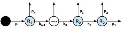
Figure 14: Illustration of the subsequent decay of an initial state (black dot) into $n$ particles. The initial state may consist of $m$ particles as only the invariant mass is relevant for the phase-space integral due to Lorentz invariance.

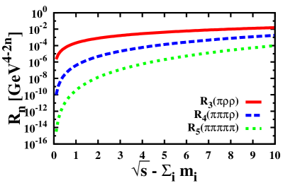
Figure 15: (Color online) Illustration of the 3-, 4-, and 5-body phase-space integrals as a function of the invariant energy above threshold. The red solid line shows the 3-body phase-space integral for $\pi\rho\rho$, the blue dashed line shows the 4-body phase-space integral for $3\pi\rho$ and the green dashed line shows the 5-body phase-space integral for 5 pions.

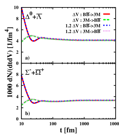
Figure 16: (Color online) Concistency check for a change in the cell size $\Delta V$ by 20%. a) for $\Delta^{0}+\bar{\Lambda}$ and b) for $\Sigma^{-}+\bar{\Omega}^{+}$ initalizations. The red solid line shows the baryon-antibaryon annihilation for the cell volume $\Delta V$, the green dashed line shows the baryon-antibaryon formation for $\Delta V$, the blue short-dashed line shows the baryon-antibaryon annihilation for $1.2\Delta V$ and the violet dotted line shows the baryon-antibaryon formation for $1.2\Delta V$.

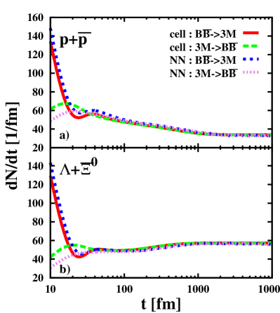
Figure 17: (Color online) Comparison of the reaction rates between the cell algorithm (cell) and the next-neighbor (NN) realization of the in-cell method. The systems shown are in a) the $p+\bar{p}$ and in b) the $\Lambda+\bar{\Xi}^{0}$ initialization. The red solid line shows the baryon-antibaryon annihilation for the cell method, the green dashed line shows the baryon-antibaryon formation for the cell method, the blue short-dashed line shows the baryon-antibaryon annihilation for the NN method and the violet dotted line shows the baryon-antibaryon formation for the NN method.

For the sake of completeness, we start with the 1-body phase-space integral,

$$R_{1}(\sqrt{s};m)=\frac{1}{(2\pi)^{3}}\int\frac{\mathrm{d}^{3}p}{2E}\leavevmode\nobreak\ (2\pi)^{4}\delta^{4}(\sqrt{s}-E)=\frac{\pi}{\sqrt{s}},$$ (18)

where E is the on-shell energy $E=\sqrt{m^{2}+p^{2}}$ and the mass $m$ of the particle is equal to the invariant energy $\sqrt{s}$. This result shows that the 1-body phase-space decreases with increasing $\sqrt{s}$. The 2-body phase space can also be evaluated analytically,

$$\begin{split}R_{2}&(\sqrt{s};m_{1},m_{2})=\\ &\leavevmode\nobreak\ \frac{1}{(2\pi)^{2}}\int\int\frac{\mathrm{d}^{3}p_{1}}{2E_{1}}\frac{\mathrm{d}^{3}p_{2}}{2E_{2}}\leavevmode\nobreak\ \delta^{3}(\vec{p}_{1}+\vec{p}_{2})\delta(\sqrt{s}-E_{1}-E_{2})\end{split}$$ (19)

$$= \frac{1}{4(2\pi)^{2}}\int\frac{\mathrm{d}^{3}p_{1}}{E_{1}E_{2}}\delta(\sqrt{s}-E_{1}-E_{2})$$ (20)

$$= \frac{1}{4(2\pi)^{2}}\int\limits_{0}^{\infty}\int\limits_{0}^{\pi}\int\limits_{0}^{2\pi}\frac{\mathrm{d}\phi\mathrm{d}\theta\mathrm{d}p_{1}\leavevmode\nobreak\ p_{1}^{2}\sin\theta}{E_{1}E_{2}}\delta(\sqrt{s}-E_{1}-E_{2})$$ (21)

$$= \frac{1}{4\pi}\int\limits_{0}^{\infty}\frac{\mathrm{d}p_{1}\leavevmode\nobreak\ p_{1}^{2}}{\sqrt{m_{1}^{2}+p_{1}^{2}}\sqrt{m_{2}^{2}+p_{1}^{2}}}\delta\left(\sqrt{s}-E_{1}-E_{2}\right).$$ (22)

The zeroes of the delta function are given by

$$p_{0}=\pm\frac{\sqrt{\lambda(s,m_{1}^{2},m_{2}^{2})}}{2\sqrt{s}},$$ (23)

where only the positive value has to be taken in our calculation. Rewriting the delta function as

$$\delta(\sqrt{s}-E_{1}-E_{2})=\frac{\delta(p_{1}-p_{0})}{p_{1}/E_{1}+p_{1}/E_{2}}$$ (24)

and plugging Eqs. (23) and (24) into Eq. (22) we obtain the two-body phase-space integral

$$\begin{split}R_{2}(\sqrt{s};m_{1},m_{2})=&\frac{1}{4\pi}\int\limits_{0}^{\infty}\frac{\mathrm{d}p_{1}\leavevmode\nobreak\ p_{1}}{E_{1}E_{2}}\frac{E_{1}E_{2}\delta(p_{1}-p_{0})}{E_{1}+E_{2}}\\ =&\frac{\sqrt{\lambda(s,m_{1}^{2},m_{2}^{2})}}{8\pi s},\end{split}$$ (25)

with $E_{1}+E_{2}=\sqrt{s}$ from the original delta function. The typical shape of $R_{2}(\sqrt{s},m_{1},m_{2})$ is shown in Fig. 13 for the masses $m_{1}=1$ GeV and $m_{2}=2$ GeV as a function of the invariant energy above threshold. The upper limit is independent of the masses and is given by $1/8\pi$.

The on-shell three-body phase-space integral $R_{3}(\sqrt{s},m_{1},m_{2},m_{3})$ is the most important one for our work and a good example for the evaluation of phase-space integrals of higher order since the $n$-body decay can be considered as consecutive 2-body decays, see Fig. 14 for an illustration. Note that in Fig. 14 $k_{n}=p$ and $k_{1}=p_{1}$. A prerequisite in calculating the phase-space integral is that we do not have any incoming momenta in between the first and final 2-body decay. For the calculation of the process we employ the recursion relation for phase-space integrals,

$$R_{n}(P)=\int\frac{\mathrm{d}^{4}p_{n}}{(2\pi)^{3}}\rho_{n}(p_{n})R_{n-1}(P-p_{n}),$$ (26)

and also insert two identities

$$1= \int\mathrm{d}M_{n-1}^{2}\delta(M_{n-1}^{2}-k_{n-1}^{2})),$$ (27)

$$1= \int\mathrm{d}^{4}k_{n-1}\delta^{4}(P-p_{n}-k_{n-1}).$$ (28)

The first identity from Eq. (27) gives the mass of the first cluster from which the 4-momentum $p_{n}$ splits. The second identity ensures energy-momentum conservation in the splitting process. Plugging both identities into Eq. (26) we find

$$R_{n}(P)= \int\mathrm{d}M^{2}_{n-1}\underbrace{\int\mathrm{d}^{4}k_{n-1}\int\frac{\mathrm{d}^{4}p_{n}}{(2\pi)^{3}}\delta^{4}(k_{n-1}^{2}-M_{n-1}^{2})\delta^{4}(p_{n}^{2}-m_{n}^{2})\delta^{4}(P-p_{n}-k_{n-1})}_{R_{2}(P;m_{n},M_{n-1})/(2\pi)}R_{n-1}(k_{n-1})$$ (29)

$$= \int\limits_{(\sum_{i=1}^{n-1}m_{i})^{2}}^{(M_{n}-m_{n})^{2}}\mathrm{d}M^{2}_{n-1}\frac{R_{2}(P;m_{n},M_{n-1})}{2\pi}R_{n-1}(k_{n-1}).$$ (30)

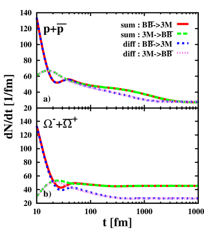
Figure 18: (Color online) Comparison of the reaction rate between the sum and the difference of the strange and antistrange quarks in the calculation of transition probabilities in $B\bar{B}\leftrightarrow 3M$ reactions (denoted by sum and diff). a) shows the $p+\bar{p}$ and b) the $\Omega^{-}+\bar{\Omega}^{+}$ initialization. The red solid line shows the baryon-antibaryon annihilation of the sum, the green dashed line shows the baryon-antibaryon formation of the sum, the blue short-dashed line shows the baryon-antibaryon annihilation of the difference and the violet dotted line shows the baryon-antibaryon formation of the difference.

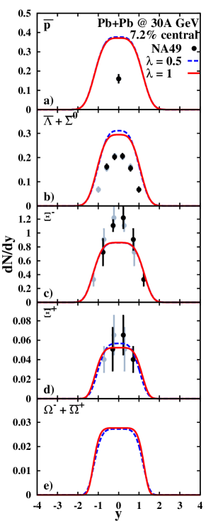
Figure 19: (Color online) Rapidity spectra for a central Pb+Pb collision at 30$A$ GeV; comparison between simulations with a strangeness suppression factor $\lambda=0.5$ (dashed lines) and no strangeness suppression, i.e. $\lambda=1$ (solid lines).

With this expression any $n$-particle phase-space integral can be calculated in a straight forward fashion as long as the masses $m_{i}$ are known. Note that the last $R_{2}$, which one gets after applying Eq. (30) several times, has no additional factor $1/(2\pi)$. In Fig. 15 the phase-space integrals for 3, 4 and 5 particles are shown as a function of the invariant energy above threshold for our example of initial $\pi\rho\rho$ with a subsequent decay into $3\pi\rho$ and a final decay to 5 pions. All phase-space integrals share a similar shape, only the magnitudes close to threshold vary substantially with the number of particles.

Appendix C In-cell method: cell-size dependence

We here show the stability of our approach with respect to the equilibrium state when changing the size of the cells. For this investigation we keep the time step d$t$ constant but enhance the cell volume $\Delta V$ by 20% and compare the reaction rate as a function of time to the default calculations in Fig. 16. We observe that the change in the cell size does not have any impact on the equilibration at all. For all times both cell sizes produce the same results giving testimony to the stability of the numerical implementation.

Appendix D In-cell method versus next-neighbor interaction

The in-cell method used for the description of the $B\bar{B}\leftrightarrow 3M$ reactions has been implemented cutting effectively the space-time into cells of cell-size $\Delta V\times\Delta t$ and letting only particles of the same cell interact with each other. Another possibility for the implementation of the baryon-antibaryon annihilation (and recreation) is by defining the volume $\Delta V$ by a sphere around the first particle and letting all particles in the sphere interact with each other; this implementation we denote by next-neighbor (NN) algorithm in the following. In Fig. 17 we compare the results of these two choices. Due to the large finite size effects for the NN method the volume of the box had to be enhanced and filled with the same density as the standard box but letting only the particles inside the standard box volume be the particles from whose sphere the partners are selected. After employing this minimization of finite size effects we find that both methods give the same reaction rates for times larger than $\approx$30 fm. A small deviation between both methods is seen for smaller times. As expected one might use in general also the NN method. The disadvantage of the numerical implementation of the NN method is the larger computational time in comparison to the discretization of space-time. Thus PHSD uses the in-cell method not for the individual cells from the NN method but for the fixed cells of the space-time discretization.

Appendix E Strangeness suppression

A further point to discuss in our model is whether to use the sum or the difference of the number of strange and anti-strange quarks in Eq. (9) for the strangeness suppression. Fig. 18 illustrates the deviation between the two suppression models for the total reaction rate. For the system consisting initially only of light quarks, $p+\bar{p}$, we see no sizeable differences between the sum and the difference of strange and anti-strange quarks in Eq. (9). The system with an initial large difference between the number of strange and anti-strange quarks, $\Omega^{-}+\bar{\Omega}^{+}$, converges to rather different equilibrium states for the two assumptions. The suppression with the sum leads to an overall larger total reaction rate and its equilibrium value is twice as large as the suppression with the difference assumption. However, both models produce rather similar results for times $t<50$ fm, which is of relevance for the heavy-ion collisions considered in this work. Accordingly we use in PHSD the suppression with the sum of the number of strange and anti-strange quarks since both models give practically identical results in PHSD simulations of relativistic heavy-ion reactions.

Another issue relates to the actual value of the strangeness suppression factor $\lambda$ which had been taken as $\lambda$ = 0.5. In order to demonstrate the impact of the parameter $\lambda$ on antibaryon spectra we show in Fig. 19 the rapidity distributions for central Pb+Pb collisions at 30 A GeV for $\lambda$=0.5 (dashed lines) and $\lambda$=1 (solid lines). Without strangeness suppression in $2\leftrightarrow 3$ reactions for hadrons with strange/antistrange quarks we find at 30$A$ GeV that the rapidity spectra of $\bar{\Lambda}+\bar{\Sigma}^{0}$ and $\bar{\Xi}^{+}$ are slightly shifted to lower values and broadened in comparison to the standard value of $\lambda=0.5$. The spectrum for $\Omega^{-}+\bar{\Omega}^{+}$ very slightly broadens and the $\bar{p}$ spectrum is basically not influenced by the change of $\lambda$.

References

- (1) Y. Aoki et al., Phys. Lett. B 643, 46 (2006).
- (2) S. Borsanyi et al., JHEP 1009, 073 (2010); JHEP 1011, 077 (2010); JHEP 1208, 126 (2012).
- (3) S. Borsanyi et al., Phys. Lett B 730, 99 (2014); Phys. Rev. D 92, 014505 (2015).
- (4) P. Petreczky [HotQCD Collaboration], PoS LATTICE 2012, 069 (2012); AIP Conf. Proc. 1520, 103 (2013).
- (5) H.-T. Ding, F. Karsch, and S. Mukherjee, Int. J. Mod. Phys. E 24, 1530007 (2015).
- (6) A. Bazavov et al., Phys. Rev. D 90, 094503 (2014).
- (7) P. Senger et al., Lect. Notes Phys. 814, 681 (2011).
- (8) F. Becattini et al., Phys. Rev. C 85, 044921 (2012); Phys. Rev. Lett. 111, 082302; Phys. Lett. B 764, 241 (2017).
- (9) J. Rafelski and B. Müller, Phys. Rev. Lett. 48, 1066 (1982) Erratum: [Phys. Rev. Lett. 56, 2334 (1986)].
- (10) P. Koch, B. Müller and J. Rafelski, Phys. Rept. 142, 167 (1986).
- (11) S. Soff, S. A. Bass, M. Bleicher, L. Bravina, M. Gorenstein, E. Zabrodin, H. Stöcker, and W. Greiner, Phys. Lett. B 471,89 (1999).
- (12) W. Cassing, A. Palmese, P. Moreau, and E. L. Bratkovskaya, Phys. Rev. C 93, 014902 (2016).
- (13) E. L. Bratkovskaya, W. Cassing, P. Moreau, and A. Palmese, Eur. Phys. J. A 52, 219 (2016).
- (14) A. Palmese, W. Cassing, E. Seifert, T. Steinert, P. Moreau and E. L. Bratkovskaya, Phys. Rev. C 94, 044912 (2016).
- (15) H. Suganuma, T. M. Doi, K. Redlich, and C. Sasaki, J. Phys. G 44, 124001 (2017).
- (16) C. Blume and C. Markert, Prog. Part. Nucl. Phys. 66, 834 (2011).
- (17) R. Stock, J. Phys. G 28, 1517 (2002).
- (18) S. Pal, C. M. Ko, and Z.-W. Lin, Nucl. Phys. A 730, 143 (2004).
- (19) S. Pal, C. M. Ko, J. M. Alexander, P. Chung, and R. A. Lacey, Phys. Lett. B 595, 158 (2004).
- (20) W. Cassing, Nucl. Phys. A 700, 618 (2002).
- (21) W. Cassing and E. L. Bratkovskaya, Phys. Rep. 308, 65 (1999).
- (22) W. Cassing and E. L. Bratkovskaya, Phys. Rev. C 78, 034919 (2008).
- (23) W. Cassing and E. Bratkovskaya, Nucl. Phys. A 831, 215 (2009).
- (24) E. L. Bratkovskaya, W. Cassing, V. P. Konchakovski and O. Linnyk, Nucl. Phys. A 856, 162 (2011).
- (25) O. Linnyk, E. L. Bratkovskaya, and W. Cassing, Prog. Part… Nucl. Phys. 87, 50 (2016).
- (26) O. Linnyk, V. Konchakovski, T. Steinert, W. Cassing and E. L. Bratkovskaya, Phys. Rev. C 92, 054914 (2015).
- (27) V. P. Konchakovski, E. L. Bratkovskaya, W. Cassing, V. D. Toneev, S. A. Voloshin and V. Voronyuk, Phys. Rev. C 85, 044922 (2012).
- (28) H. Petersen, M. Bleicher, S. A. Bass and H. Stöcker, arXiv:0805.0567 [hep-ph].
- (29) Y. B. Ivanov, Phys. Rev. C 87, 064905 (2013).
- (30) L. P. Kadanoff and G. Baym, Quantum Statistical Mechanics (Benjamin, New York, 1962).
- (31) J. S. Schwinger, J. Math. Phys. 2, 407 (1961).
- (32) L. V. Keldysh, Sov. Phys. JETP 20, 1018 (1965).
- (33) W. Botermans and R. Malfliet, Phys. Rept. 198, 115 (1990).
- (34) W. Cassing and S. Juchem, Nucl. Phys. A 665, 377 (2000).
- (35) W. Cassing and S. Juchem, Nucl. Phys. A 672, 417 (2000).
- (36) S. Juchem, W. Cassing and C. Greiner, Phys. Rev. D 69, 025006 (2004).
- (37) A. Peshier, Phys. Rev. D 70, 034016 (2004).
- (38) A. Peshier, J. Phys. G 31, S371 (2005).
- (39) A. Peshier and W. Cassing, Phys. Rev. Lett. 94, 172301 (2005).
- (40) W. Cassing, E. Phys. J. ST 168, 3 (2009).
- (41) V. Ozvenchuk et al., Phys. Rev. C 87, 024901 (2013).
- (42) W. Cassing et al., Phys. Rev. Lett. 110, 182301 (2013).
- (43) T. Steinert and W. Cassing, Phys. Rev. C 89, 035203 (2014).
- (44) B. Nilsson-Almqvist and E. Stenlund, Comput. Phys. Commun. 43, 387 (1987).
- (45) C. H. Li and C. M. Ko, Nucl. Phys. A 712,110 (2002).
- (46) F. Li, L. W. Chen, C. M. Ko and S. H. Lee, Phys. Rev. C 85, 064902 (2012).
- (47) V. Flaminio, W. G. Moorhead, D. R. O. Morrison, and N. Rivoire, CERN-HERA-83-02.
- (48) V. D. Toneev, V. Voronyuk, E. E. Kolomeitsev, and W. Cassing, Phys. Rev. C 95, 034911 (2017).
- (49) E. Byckling and K. Kajantie, Particle Kinematics (John Wiley & Sons Ltd, 1973).
- (50) T. Sjostrand, S. Mrenna, and P. Z. Skands, JHEP 0605, 026 (2006).
- (51) K. A. Olive et al. [Particle Data Group], Chin. Phys. C 38, 090001 (2014).
- (52) A. Lang, H. Babovsky, W. Cassing, U. Mosel, H.-G. Reusch and K. Weber, Journal of Computational Physics 106, 391 (1993).
- (53) Z. Xu and C. Greiner, Phys. Rev. C 71, 064901 (2005).
- (54) B. B. Back et al. [E917 Collaboration], Phys. Rev. Lett. 87, 242301 (2001).
- (55) T. Anticic et al. [NA49 Collaboration], Phys. Rev. C 83, 014901 (2011).
- (56) C. Alt et al. [NA49 Collaboration], Phys. Rev. C 78, 034918 (2008).
- (57) C. Alt et al. [NA49 Collaboration], Phys. Rev. Lett. 94, 192301 (2005).
- (58) C. Alt et al. [NA49 Collaboration], Phys. Rev. C 73, 044910 (2006).
- (59) S. A. Bass et al., Prog. Part. Nucl. Phys. 41, 255 (1998).
- (60) M. Bleicher et al., J. Phys. G 25, 1859 (1999).
- (61) Yu. B. Ivanov, V. N. Russkikh, and V. D. Toneev, Phys. Rev. C73, 044904 (2006); V. N. Russkikh, and Yu. B. Ivanov, Phys. Rev. C 74, 034904 (2006); Yu. B. Ivanov, Phys. Rev. C 87, 064904 (2013); Yu. B. Ivanov and D. Blaschke, Phys. Rev. C 92, 024916 (2015).