Role of three-particle vertex within dual fermion calculations

Abstract

We investigate the influence of self-energy diagrams beyond the two-particle vertex level within dual fermion theory. Specifically, we calculate the local three-particle vertex and construct from it selected dual fermion self-energy corrections to dynamical mean field theory. For the two-dimensional Hubbard model, the thus obtained self-energy corrections are small in the parameter space where dual fermion corrections based on the two-particle vertex only are small. However, in other parts of the parameter space, they are of a similar magnitude and qualitatively different from standard dual fermion theory. The high-frequency behavior of the self-energy correction is – surprisingly – even dominated by corrections stemming from the three-particle vertex.

I Introduction

Strongly correlated electron systems pose some of the greatest challenges in modern solid-state theory. The interplay between the interaction that is diagonal in real space and the kinetic energy that is diagonal in momentum space causes some fascinating, albeit hard to describe physical phenomena. Analytical solutions to interacting lattice fermion systems are scarce and numerical treatments have to face the exponential growth of the Hilbert space with the number of lattice sites. Quantum Monte Carlo methods, for their part, suffer from the fermionic sign problem. In this situation, dynamical mean field theory (DMFT)(Metzner89a, ; MuellerHartmann89, ; Georges92a, ) has become a standard method for the treatment of correlation effects in fermionic lattice systems. By considering local correlations only, DMFT self-consistently maps the lattice problem onto a single-site Anderson impurity model. This model can be solved reliably by a variety of algorithms. Often continuous-time quantum Monte Carlo (CT-QMC) simulations Rubtsov2005 ; Werner2006 ; Gull2008a ; Gull2011a are employed to this end because of their robustness, versatility, and the ability to treat continuous baths.

Nevertheless, DMFT is limited to local correlation effects by construction. Hence, more recently, diagrammatic extensions of DMFT have been at the focus of intense research efforts. These methods aim to utilize the well-established local quantities derived from DMFT as a starting point but add, on top of these, non-local correlations by means of Feynman diagrams. Examples of such diagrammatic extensions of DMFT are the dynamical vertex approximation (D$\Gamma$A)(DGAintro, ; DGA, ), the dual fermion (DF)(DF, ) theory and the one-particle-irreducible approach (1PI)(1PI, ) to mention just some of them; for a review see Ref. RMPVertex, . A common feature of all diagrammatic extensions is that they build upon the local (two- and more-particle) vertex and use it to construct non-local correlations in one- and two-particle quantities. These approaches allow for describing physical phenomena beyond the realm of DMFT, such as formation of a pseudogap Katanin2009 ; Rubtsov2009 ; Jung2010 ; Jung2011 ; Taranto2014 ; Schaefer2015-2 and (quantum) critical exponents Rohringer2011 ; Antipov2014 ; Hirschmeier2015 ; Schaefer2016 .

The mentioned diagrammatic extensions (D$\Gamma$A, DF and 1PI) should – in principle – include local vertex functions up to infinite order in the particle number. However, hitherto the application of these theories has been mostly restricted to the two-particle level. On the one hand it was argued that most of the relevant physics such as spin fluctuations should already be included in diagrams generated from the two-particle vertex (indeed in weak coupling perturbation theory this physics is generated from similar diagrams with the bare two-particle interaction instead of the vertex). On the other hand, a very practical reason for the truncation at the level of the two-particle vertex exists: three-particle vertices are numerically very expensive to calculate and only recently enhanced computer resources and improved algorithms made such calculations feasible. Furthermore, three-particle diagrammatics is much more complicated to treat (also combinatorically) than two-particle diagrammatics.

To the best of our knowledge, there are only two previous papers that include higher-order vertices within the DF framework. Ref. Hafermann2009, found only weak effects of selected low-order diagrams on the leading eigenvalue of the Bethe-Salpeter equation in the dual $ph$-channel for the Hubbard model. In contrast, Ref. Ribic2017, identified strong self-energy corrections due to the three-particle vertex in the Falicov-Kimball model.

It is the aim of this paper to further elucidate and to estimate the influence of higher order vertex correlations on the self-energy within DF. To this end, we calculate local three-particle vertices using CT-QMC. From these we evaluate a simple self-energy diagram and investigate its contribution in comparison to DMFT, the dynamical cluster approximation (DCA), standard DF, 1PI and D$\Gamma$A.

The study is conducted for the Hubbard model with nearest neighbor hopping $t$ and interaction $U$ on a square lattice which is described by the Hamiltonian

$${\mathcal{H}}=-t\sum_{\langle ij\rangle,\sigma}{c}_{i\sigma}^{\dagger}{c}_{j\sigma}^{\phantom{\dagger}}+U\sum_{i}{c}_{i\uparrow}^{\dagger}{c}_{i\uparrow}^{\phantom{\dagger}}{c}_{i\downarrow}^{\dagger}{c}_{i\downarrow}^{\phantom{\dagger}}$$ (1)

Here, $\langle ij\rangle$ denotes the summation over pairs of nearest neighbor sites $i$ and $j$; and ${c}_{i\sigma}^{({\dagger})}$ annihilates (creates) an electron on site $i$ with spin $\sigma$. In the following, the half-bandwidth ($4t$) is chosen as the unit of energy, i.e., $4t\equiv 1$.

The outline of the paper is as follows: Section II is devoted to the calculation of the local three-particle vertex. In Section II.1, the form of this three-particle vertex and how to obtain it from the three-particle Green’s function by subtracting disconnected contributions and amputating Green’s functions is discussed. The CT-QMC calculation of the three-particle Green’s functions is outlined in turn in Section II.2, with additional information in Appendix A. The Feynman diagrams that we consider in DF with this three-particle vertex as a starting point and the corresponding equations are given in Section III. This is supplemented in Appendix B by a derivation of a generalized Schwinger-Dyson equation. Section IV presents the results obtained for the two-dimensional Hubbard model. Finally, Section V provides a summary and an outlook.

II Calculation of local three-particle quantities within DMFT

II.1 Three-particle Green’s function and vertex

Let us start by formally defining the local three-particle Green’s function

$$G_{\nu_{1}\nu\nu^{\prime}\omega}^{(3)\sigma_{1}\sigma_{2}\sigma_{3}}=\langle{c}_{\sigma_{1}}^{\dagger}(\nu_{1}){c}_{\sigma_{1}}(\nu_{1})\times\\ {c}_{\sigma_{2}}^{\dagger}(\nu-\omega){c}_{\sigma_{2}}(\nu){c}_{\sigma_{3}}^{\dagger}(\nu^{\prime}){c}_{\sigma_{3}}(\nu^{\prime}-\omega)\rangle,$$ (2)

with three fermionic Matsubara frequencies $\nu_{1},\nu,\nu^{\prime}$ and one bosonic (transfer) frequency $\omega$, cf. Appendix A for the Fourier-transformation from imaginary times. Fig. 1 illustrates our frequency- and spin-convention for three-particle quantities.

To obtain the fully connected $n$-particle vertex functions $F^{(n)}$ from $G^{(n)}$, first any disconnected contribution to the propagators needs to be removed. Subsequently we need to amputate the outer legs of the remaining, fully connected three-particle Green’s function $G_{C}^{(n)}$. On the two-particle level, there are only two disconnected contributions to the Green’s function $G^{(2)}$, both consisting of a product of two one-particle Green’s functions: $G^{(1)}G^{(1)}$. On the three-particle level, there is much more variety among the disconnected terms. A three-particle Green’s function $G^{(3)}$ contains terms disconnected into three one-particle propagators, $G^{(1)}G^{(1)}G^{(1)}$ (for example $\delta_{\omega,0}\ G_{\nu_{1}}^{(1)\sigma_{1}}G_{\nu}^{(1)\sigma_{2}}G_{\nu_{3}}^{(1)\sigma_{3}}$), as well as other terms disconnected into a one-particle and a connected two-particle Green’s function, $G^{(1)}G_{C}^{(2)}$ (for example $G_{\nu_{1}}^{(1)\sigma_{1}}G_{C\ \nu\nu^{\prime}\omega}^{(2)\sigma_{2}\sigma_{3}}$), as well as a fully connected term, see Fig. 2 for an illustration.

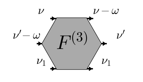
Figure 1: Frequency convention for the three-particle vertex $F^{(3)}$. Note that we consider throughout the paper the situation where no energy is transferred to frequency $\nu_{1}$ which reduces the frequency dependence of $F^{(3)}$ to four frequencies. As for spin degrees of freedom, $F^{\sigma_{1}\sigma_{2}\sigma_{3}}$ denotes the vertex component where both lines associated with frequency $\nu_{1}$ carry the spin $\sigma_{1}$, the lines associated with $\nu$ carry $\sigma_{2}$ and the lines associated with $\nu^{\prime}$ carry $\sigma_{3}$.

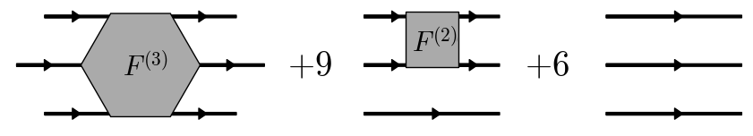
Figure 2: The three-particle Green’s function $G^{(3)}$ is decomposed into a three-particle connected contribution [$G_{C}^{(3)}=G^{(1)}G^{(1)}G^{(1)}F^{(3)}G^{(1)}G^{(1)}G^{(1)}$], nine terms consisting of a one-particle and connected two-particle Green’s functions [$G^{(1)}G_{C}^{(2)}$], and six disconnected contributions [$G^{(1)}G^{(1)}G^{(1)}$].

II.2 CT-QMC results for the local three-particle vertex functions

Continuous-time quantum Monte Carlo (CT-QMC) algorithms are based on a series expansion of the partition function, and here employed for the Anderson impurity model. While the specific Green’s function measurement depends on the choice of expansion, CT-QMC algorithms in general provide $n$-particle Green’s functions, consisting of fully connected as well as disconnected contributions. Extracting irreducible vertex functions by subtracting disconnected contributions and amputating outer legs, as discussed in the previous Section, is a post-processing step to the simulation. CT-QMC algorithms natively operate in the imaginary time domain. It is thus necessary to define a suitable Fourier transform to recover the Matsubara frequency representation of Eq. (2).

Here, we calculate the three-particle Green’s function for the auxiliary AIM associated to a DMFT solution at self-consistency, using both, CT-QMC in the hybridization expansion (CT-HYB)Werner2006 and in the auxiliary field expansion (CT-AUX).Gull2008 While in CT-AUX the single-particle Green’s function $G_{\nu}^{loc}$ is measured as a correction to the non-interacting Green’s function $G_{0}$, in CT-HYB the measurement is achieved by cutting hybridization lines, not correcting any prior Green’s function object. In CT-AUX, corrections hence converge rapidly in the high-frequency regions ($\sim 1/\nu^{2}$), while the CT-HYB result displays a constant error over the entire frequency range. This becomes much more relevant for the vertex where we have, as discussed, to amputate Green’s function lines. This corresponds to a division by a small number at large frequencies. Hence the CT-HYB three-particle vertex is noisy at larger frequencies, even more so than the two-particle vertex. This makes weak-coupling CT-QMC algorithms (e.g. CT-AUX) more suitable for the calculation of the vertex than strong-coupling algorithms (i.e. CT-HYB), at least when applied to single-orbital models. However, we note that the high-frequency behavior of CT-HYB algorithms is greatly alleviated by employing improved estimators on the one-particle level Hafermann2012 or vertex asymptotics on the two-particle level.Kaufmann2017 Moreover, when eventually calculating the self-energy, the aforementioned small Green’s functions are multiplied again so that the noise at high-frequencies has a negligible effect for calculations based on the two-particle vertex.JPSJ-XXX As we will see below this remains true for three-particle vertex corrections to the self-energy, but here only for the lowest few Matsubara frequencies.

of DMFT. Fig. 3 shows the local three-particle CT-AUX vertex calculated for the impurity problem of the DMFT solution for the Hubbard-model at $U=1$, inverse temperature $\beta=8$, and half-filling $n=1$. With the frequency $\nu_{1}$ fixed, the local three-particle vertex displays features very similar to a two-particle vertex. A cross-like structure is visible along the diagonal $\nu=\nu^{\prime}$ and the secondary diagonal $\nu=-\nu^{\prime}+\omega$. A plus-like structure extends from $\nu=\pm\pi/\beta$ and $\nu^{\prime}=\pm\pi/\beta$ as well as $\nu-\omega=\pm\pi/\beta$ and $\nu^{\prime}-\omega=\pm\pi/\beta$. The features of the vertex are more pronounced for $\nu=+\pi/\beta=\nu_{1}$, $\nu^{\prime}=+\pi/\beta=\nu_{1}$ etc. than for $\nu=-\pi/\beta=-\nu_{1}$, $\nu^{\prime}=-\pi/\beta=-\nu_{1}$. Additionally, a constant background is present. The observed structure is to be expected, as plotting the three-particle vertex along the $\nu_{1}$ diagonal can be physically interpreted as the scattering amplitude of a particle with energy $\nu_{1}$ with a particle and a hole at energies $\nu,\nu^{\prime}$ scattering with a transfer frequency $\omega$.

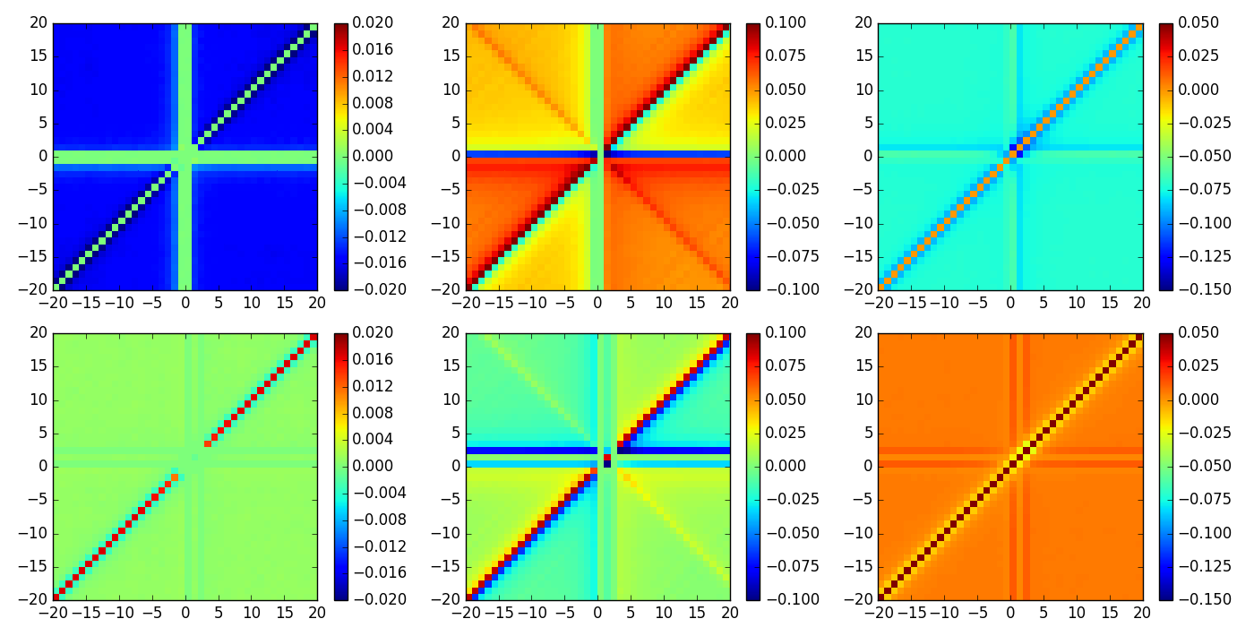
Figure 3: Full three-particle vertex $F^{\sigma_{1}\sigma\sigma^{\prime}}$ (imaginary part) for the parameters $U=1,\beta=8$ and $n=1$. The frequency $\nu_{1}$ was set to the first fermionic Matsubara frequency. The heatplots are given as functions of Matsubara frequency $n_{\nu}$ and $n_{\nu}^{\prime}$ [$\nu=(2n_{\nu}+1)\pi/\beta$] for $\omega=0$ (upper row) and $\omega=4\pi/\beta$ (lower row) for the spin configurations $\sigma_{1}\sigma\sigma^{\prime}=\uparrow\uparrow\uparrow$ (left), $\sigma_{1}\sigma\sigma^{\prime}=\uparrow\uparrow\downarrow$ (centre) and $\sigma_{1}\sigma\sigma^{\prime}=\uparrow\downarrow\downarrow$ (right).

III Dual fermion approach up to third order

The dual fermion approach allows for a systematic and – in principle – exact decoupling of local and non-local degrees of freedom for interacting lattice problems. This is achieved by a Hubbard-Stratonovich transformation, which yields a so-called dual action of the form (see Ref. RMPVertex, ):

$$\mathcal{S}_{dual}\left[\tilde{c}^{{\dagger}};\tilde{c}^{\phantom{{\dagger}}}\!\right]=\sum_{k_{1}}\dfrac{1}{G_{{\mathbf{k}}}-G_{\nu}^{loc}}\tilde{c}_{k_{1}}^{{\dagger}}\tilde{c}_{k_{1}}^{\phantom{{\dagger}}}+\\ \sum_{n=2}^{\infty}\sum_{{k_{1}},{k_{2}},{k_{3}},{k_{4}},...}\dfrac{1}{(n!)^{2}}F^{(n)}({k_{2}},{k_{1}},{k_{4}},{k_{3}},...)\tilde{c}_{k_{2}}^{\phantom{{\dagger}}}\tilde{c}_{k_{1}}^{{\dagger}}\tilde{c}_{k_{4}}^{\phantom{{\dagger}}}\tilde{c}_{k_{3}}^{{\dagger}}...$$ (3)

Here, the Grassmann fields $\tilde{c}^{({\dagger})}$ are associated with the dual fermion degrees of freedom, and we use a four-vector plus spin notation $k=({\mathbf{k}},\nu,\sigma)$. $G_{\nu}^{{\rm loc}}$ is the local DMFT Green’s function and $G_{k}$ the ${\mathbf{k}}$-dependent DMFT Green’s function for the Hubbard model that is obtained from the Dyson equation and the local DMFT self-energy. The non-interacting dual Green’s function is given by $\widetilde{\mathcal{G}}_{0,k}=G_{{k}}-G_{\nu}^{{\rm loc}}$. The full $n$-particle DMFT vertex functions $F^{(n)}$ are fully local and, hence, depend only on the frequency- and spin-arguments and scatter equally between all states obeying momentum conservation.

With the action Eq. (3) as a starting point we can calculate via Feynman diagrammatic methods the interacting DF Green’s function $\widetilde{\mathcal{G}}_{k}$ and self-energy $\widetilde{\Sigma}_{k}$. As we show in Appendix B, the latter is connected to the dual $n$-particle Green’s function $\widetilde{\mathcal{G}}^{(n)}$ via a generalized Schwinger-Dyson equation (or Heisenberg equation of motion)

$$\widetilde{\Sigma}_{k}=-\sum_{n=2}^{\infty}\sum_{{k_{2}},{k_{3}},{k_{4}},...}\dfrac{(-1)^{n}}{n!(n-1)!}\\ F^{(n)}({k_{2}},k,{k_{4}},{k_{3}},...)\widetilde{\mathcal{G}}^{(n)}(k,{k_{2}},{k_{3}},{k_{4}},...)/\widetilde{\mathcal{G}}_{k}$$ (4)

Diagrammatically, the interpretation of the above equation is straightforward: any dual self-energy diagram has to start with an interaction vertex. Since there are infinitely many types of interaction vertices, an infinite sum of contributions to the self-energy exists. Note that the dual Green’s functions $\widetilde{\mathcal{G}}^{(n)}$ describe all possible diagrams which can be built from the original local vertices $F^{(n)}$. The remaining external leg $\widetilde{\mathcal{G}}_{k}$ of the dual Green’s function has to be amputated to generate a self-energy diagram.

In Eq. (4) full dual $n$-particle Green’s functions appear. (not connected ones) However, any disconnected contribution to the Green’s function where a dual one-particle Green’s function closes a loop locally does not influence the dual self-energy if the one-particle dual Green’s functions are required to be completely non-local, i.e. $\sum_{\mathbf{k}}\widetilde{\mathcal{G}}_{\mathbf{k}\nu\sigma}=0$. For this reason, e.g. no Hartree or Fock term appears for the dual fermions when truncating on the two-particle vertex level.

In this paper, we consider local interaction terms up to the three-particle vertex in Eq. (3). The actual choice of diagrams, which are constructed from these building blocks, is dictated by the physics of the system: In fact, for electrons on a bipartite lattice at (or close to) half-filling antiferromagnetic spin fluctuations are the predominant mechanism through which non-local correlations affect self-energies and spectral functions. Diagrammatically, such spin fluctuations are captured by ladder diagrams for $G^{(2)}$ (or equivalently $\widetilde{\mathcal{G}}^{(2)}$) in the $ph$ (and $\overline{ph}$) channel. Considering first Eq. (4) for $n=2$ we construct the diagram in Fig. 4. This ladder-based contribution to the dual self-energy corresponds to the standard choice for DF calculations in previous works.(Brener2008, ; Hafermann2009, ) The simplest contributions to $\widetilde{\mathcal{G}}^{(3)}$ in Eq. (4) are the disconnected ones. For $\widetilde{\mathcal{G}}^{(3)}$, an equivalent decomposition to the one in Fig. 2 exists. In order to include antiferromagnetic spin fluctuations also for $n=3$ in Eq. 4, we consider the very same ladder diagrams for the disconnected contributions to $\widetilde{\mathcal{G}}^{(3)}$. The terms of the form $\widetilde{\mathcal{G}}_{k}\widetilde{\mathcal{G}}_{k}\widetilde{\mathcal{G}}_{k}$ vanish for the same reason the Hartree- and Fock terms vanish for the two-particle vertex: a closed Green’s function loop with $\sum_{\mathbf{k}}\widetilde{G}_{\mathbf{k}\nu\sigma}=0$. The same holds for six out of the nine $\widetilde{\mathcal{G}}^{(2)}\widetilde{\mathcal{G}}_{k}$ terms contributing to $\widetilde{\mathcal{G}}^{(3)}$ analogously to the decomposition in Fig. 2. The remaining three possibilities contribute equally. Thus, within our approximation, and taking into account all combinatorical prefactors our dual self-energy from the two- and three-particle vertex reads

$$\widetilde{\Sigma}_{k}\approx-\sum_{k_{2},k_{3},k_{4}}\dfrac{1}{2}F^{(2)}(k_{2},k,k_{4},k_{3})\ \widetilde{\mathcal{G}}_{0,k_{2}}\ \widetilde{\mathcal{G}}_{0,k_{3}}\ \widetilde{\mathcal{G}}_{0,k_{4}}\ \mathcal{F}^{(2)}(k,k_{2},k_{3},k_{4})\,\\ +\sum_{k_{1},k_{2},k_{3},k_{4}}\dfrac{1}{4}F^{(3)}(k,k,k_{2},k_{1},k_{4},k_{3})\ \widetilde{\mathcal{G}}_{0,k_{1}}\ \widetilde{\mathcal{G}}_{0,k_{2}}\ \widetilde{\mathcal{G}}_{0,k_{3}}\ \widetilde{\mathcal{G}}_{0,k_{4}}\ \mathcal{F}^{(2)}(k_{1},k_{2},k_{3},k_{4}).$$ (5)

The diagrammatic representation of the first line is given in Fig. 4; it corresponds to standard DF and $n=2$ in Eq. (4). The new contribution in the second line stems from $n=3$ and is illustrated in Fig. 5. The vertex $\mathcal{F}^{(2)}$ in Eq. (5) denotes the full vertex of the dual fermions. In principle it can be obtained from the action Eq. (3) or all Feynman diagrams with ${F}^{(n)}$ and $\widetilde{\mathcal{G}}$ as building blocks. Since an exact calculation of this quantity proves elusive, further approximations are needed on its part. We employ the standard approximation to this end, the $ph$ ladder approximation for $\mathcal{F}^{(2)}$:

$$\mathcal{F}_{kk^{\prime}q,lad}^{(2)}=F_{kk^{\prime}q}^{(2)}-\sum_{k_{1}}\mathcal{F}_{kk_{1}q,lad}^{(2)}\widetilde{\mathcal{G}}_{k_{1}}\widetilde{\mathcal{G}}_{k_{1}-q}F_{k_{1}k^{\prime}q}^{(2)}.$$ (6)

Where a three-variable notation

$$\mathcal{F}_{kk^{\prime}q}^{(2)}=\mathcal{F}^{(2)}(k,k-q,k^{\prime}-q,k^{\prime})$$ (7)

was adapted.

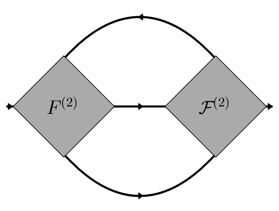
Figure 4: Feynman-diagrammatic representation of the dual self-energy in terms of the local two-particle vertex $F^{(2)}$, the dual propagator $\widetilde{\mathcal{G}}$ (line) and the full DF vertex ${\cal F}^{(2)}$ (obtained, e.g., through a ladder series).

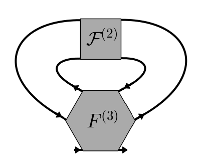
Figure 5: Feynman-diagrammatic representation of an additional contribution to the dual self-energy that includes the local three-particle vertex of the real fermions $F^{(3)}$.

The self-energy as obtained in Eq. (5) is the one for the dual electrons, i.e., it corrects the dual non-interacting Green’s function. In order to obtain from it nonlocal correlations for real electrons it has to be transformed to the space of the original particles. For this purpose, the formalism of the DF theory provides an exact relation DF which reads

$$\Sigma_{k}=\Sigma_{\nu}^{loc}+\dfrac{\widetilde{\Sigma}_{k}}{1+G_{\nu}^{loc}\widetilde{\Sigma}_{k}}.$$ (8)

While this relation certainly holds for the exact $\tilde{\Sigma}$ (i.e., where all diagrams for vertices of all orders are taken into account) it has been argued on the basis of diagrammatic considerations at weak couplingsixpoint ; 1PI ; RMPVertex that it should be modified if only certain subsets of diagrams are considered:

$$\Sigma_{k}=\Sigma_{\nu}^{{\rm loc}}+\widetilde{\Sigma}_{k},$$ (9)

The (weak-coupling) arguments in favor of Eq. (9) given in the aforementioned Refs. 1PI, ; RMPVertex, are also valid for the choice of diagrams for $\tilde{\Sigma}$ of the present paper. However, as there is no conclusive understanding regarding the choice of Eq. (8) or Eq. (9) for all coupling regimes, and an analysis of the difference between them are outside of the scope of this paper, we will consider both for the presentation of our numerical results in the next section.

IV Results: self-energy corrections

Let us now present the numerical results for one-shot DF calculations based on converged DMFT baths for the two-dimensional Hubbard model. For every discussed point, Fig. 6 shows the (Matsubara) frequency dependence of the DF self-energy correction . This self-energy needs to be added to the DMFT self-energy to obtain the physical self-energy of the Hubbard model. We compare in Fig. 6 the standard DF self-energy $\widetilde{\Sigma}_{2{\mathbf{k}}\nu}$ [first line of Eq. (4)] at the nodal $(\pi/2,\pi/2)$ and antinodal $(\pi,0)$ ${\mathbf{k}}$-point of the Fermi surface with the selected additional contribution based on the three-particle vertex [second line of Eq. (4)]. This specific three-particle correction couples the two-particle ladder diagrams with the three particle vertex, see Fig. 5, and is ${\mathbf{k}}$-independent.

Additionally, in Fig. 7 the real and imaginary part of the dual self-energy corrections is given along a path through the Brillouin zone, including as well as excluding the three-particle vertex correction. Because of its ${\mathbf{k}}$-independence, the latter just gives a constant offset in these plots. Since the DF self-energy is only a correction to the DMFT self-energy in Eq. (9), a positive imaginary part only means that the finite life time (damping) effect of DMFT is reduced. For all investigated points the physical self-energy remains negative.

Let us now discuss and interpret these results. At high temperatures [($U=1$, $\beta=8$, $n=1$) and ($U=2$, $\beta=8$, $n=1$)] and for the doped system [($U=1$, $\beta=15$, $n=0.8$)], the standard dual Fermion self-energy $\widetilde{\Sigma}_{2}$ is only a relatively small correction to the DMFT self-energy [${\rm Im}\Sigma_{n_{\nu}=1}^{{\rm loc}}$= $-0.14$, $-0.96$ and $-0.075$, respectively]. For $U=1$, the DF corrections based on the three-particle vertex $\widetilde{\Sigma}_{3}$ are again considerably smaller than $\widetilde{\Sigma}_{2}$. Note that this does not hold for all ${\mathbf{k}}$-points. For example, the scattering rate due to ${\rm Im}\widetilde{\Sigma}_{3}$ is larger than for ${\rm Im}\widetilde{\Sigma}_{2}$ for ${\mathbf{k}}=(\pi/2,\pi/2)$. But $\widetilde{\Sigma}_{2}$ is much larger for ${\mathbf{k}}=(\pi,0)$, and also in general the variation of $\widetilde{\Sigma}_{2}$ with ${\mathbf{k}}$ is much larger than $\widetilde{\Sigma}_{3}$. While the three-particle vertex corrections appear small in Fig. 7, Fig. 6 reveals that $\widetilde{\Sigma}_{3}$ is actually comparable in magnitude to $\widetilde{\Sigma}_{2}$ when taking the second (not the first) Matsubara frequency into account. This is particularly true for ($U=2$, $\beta=8$, $n=1$) which happens to have a particularly small $\widetilde{\Sigma}_{3}$ at the lowest Matsubara frequency.

We can trace these large DF contributions, both for $\widetilde{\Sigma}_{3}$ and $\widetilde{\Sigma}_{2}$, back to the strong enhancement of ${\cal F}^{2}$ in the ladder series for spin-$\uparrow\downarrow$ and ${\mathbf{q}}=(\pi,\pi)$. Physically this corresponds to strong spin fluctuations in the two-dimensional Hubbard model. For $\widetilde{\Sigma}_{2}$ these spin fluctuations combine with one more interacting vertex $F^{(2)}$ in Eq. (4) to yield a strongly ${\mathbf{k}}$-dependent self-energy and pseudogap physics. But the very same spin fluctuations also couple to the three-particle vertex in Eq. (4), and yield a ${\mathbf{k}}$-independent imaginary part of the self-energy of similar magnitude. We additionally compared the self-energies, as extracted from DMFT, dual fermion, based on two and three-particle vertices, D$\Gamma$A and DCA in Fig. 9. The results were obtained $\beta=8$. The general trend, however, of the dominant fluctuations influencing the three-particle corrections in a sizable fashion is expected to persist within a stable, self-consistent approach.

An important remark is in order regarding the $1/i\nu$ asymptotic behavior of the self-energy $\Sigma_{k}$ for the real electrons: The correction $\tilde{\Sigma}^{(3)}$ [second line in Eq.(5)] gives rise to a $1/\nu$ contribution in $\tilde{\Sigma}$ (see inset in Fig. 6, left panel). This modifies the – already correct – $1/i\nu$ asymptotics of the local DMFT self-energy and leads, hence, to a wrong $1/i\nu$ behavior of the total self-energy in Eqs. (8) or (9). Such a violation of the asymptotic behavior of the self-energy can be also observed in the D$\Gamma$A and the 1PI approaches Katanin2009 ; RohringerToschi2016 ; 1PI and can be traced back RohringerToschi2016 to a violation of the Pauli principle at the two-particle level [i.e., more precisely to a violation of the sum rule $\frac{1}{\beta}\sum_{k}\chi_{\uparrow\uparrow}^{k}=\frac{n}{2}\left(1-\frac{n}{2}\right)$] in ladder based approaches. In the D$\Gamma$A and the 1PI approach this problem has been overcome Katanin2009 ; 1PI ; RohringerToschi2016 ) by renormalizing the corresponding spin- and/or charge-susceptibilities through a Moriya $\lambda$ correction. Such a procedure could be also applied for the situation in this paper where the violation of the asymptotics of $\Sigma$ originates from the inclusion of the local three-particle vertex. An alternative route, which is more in the spirit of the DF method, would be to choose an appropriate (outer) self-consistency condition for the local reference system which removes the spurious asymptotic behavior. The question of which of the proposed methods is more suitable needs further discussions and goes beyond the scope of the present paper.

Let us note that we find good agreement between DF calculations based on vertices from CT-AUX and CT-HYB calculations, as exemplarily shown in Fig. 10, though a separate investigation of the vertices themselves showed that CT-AUX vertices display less noise, especially at high frequencies. Let us note that for higher frequencies, outside the range of Fig. 10, the CT-HYB self-energy becomes more noisy.

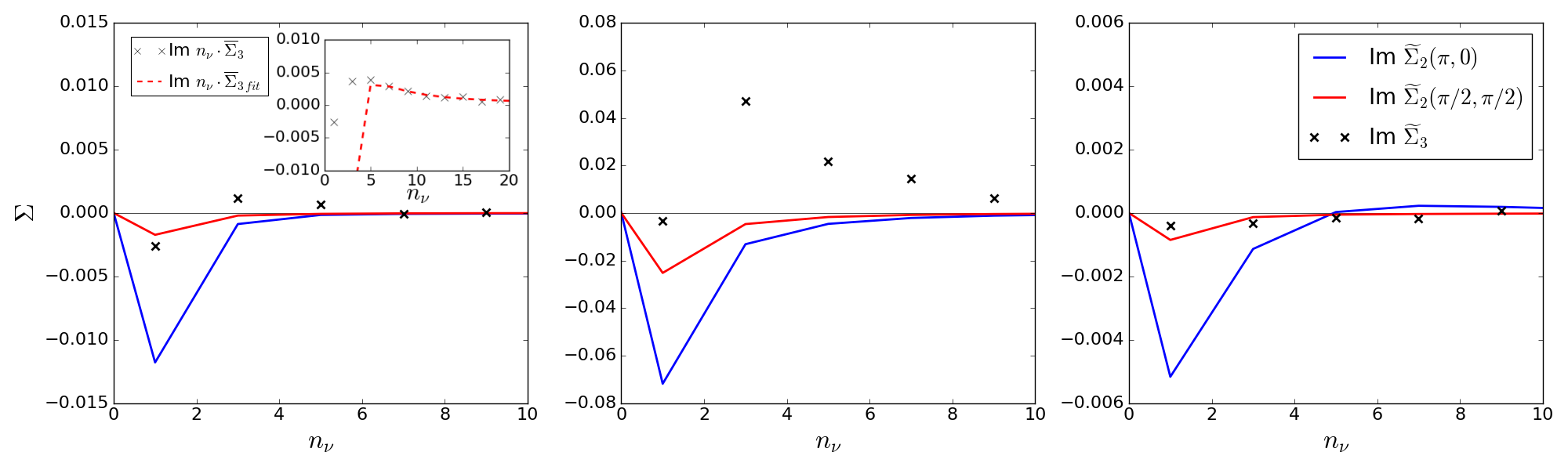
Figure 6: Imaginary part of the dual self-energy correction of the standard DF theory $\widetilde{\Sigma}_{{\mathbf{k}}\nu}$ for two ${\mathbf{k}}$-points and the correction $\widetilde{\Sigma}_{3}$ based on the three particle vertex and diagram Fig. 5. From left to right, we present data for $U=1$, $\beta=8$, $n=1$; $U=2$, $\beta=8$, $n=1$ and $U=1$, $\beta=15$, $n=0.8$, cf. phase diagram Fig. 8. Inset in the first figure shows fitting function used to estimate high-frequency behavior.

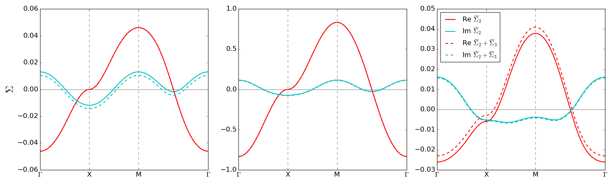
Figure 7: Same as Fig. 6 but now presenting the ${\mathbf{k}}$-dependence of the DF self-energy with ($\widetilde{\Sigma}_{2}+\widetilde{\Sigma}_{3}$) and without ($\widetilde{\Sigma}_{2}$) three-particle vertex corrections. The figure shows the imaginary and real part of the DF self-energy at the lowest Matsubara frequency along the path $\Gamma=(0,0)\rightarrow X=(\pi,0)\rightarrow M=(\pi,\pi)\rightarrow\Gamma$ through the Brillouin zone.

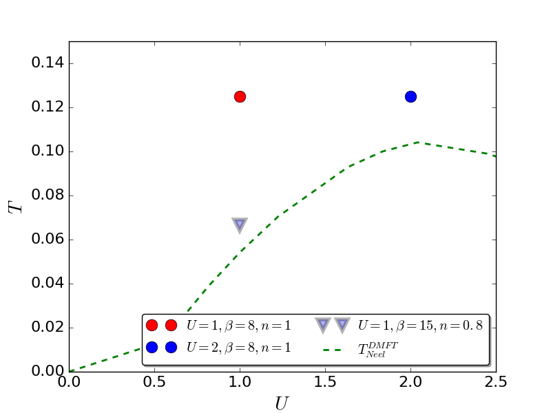
Figure 8: Positions of investigated points in parameter space relative to the Néel-temperature within DMFT for the half-filled system (which is an indication where spin fluctuations become more relevant).

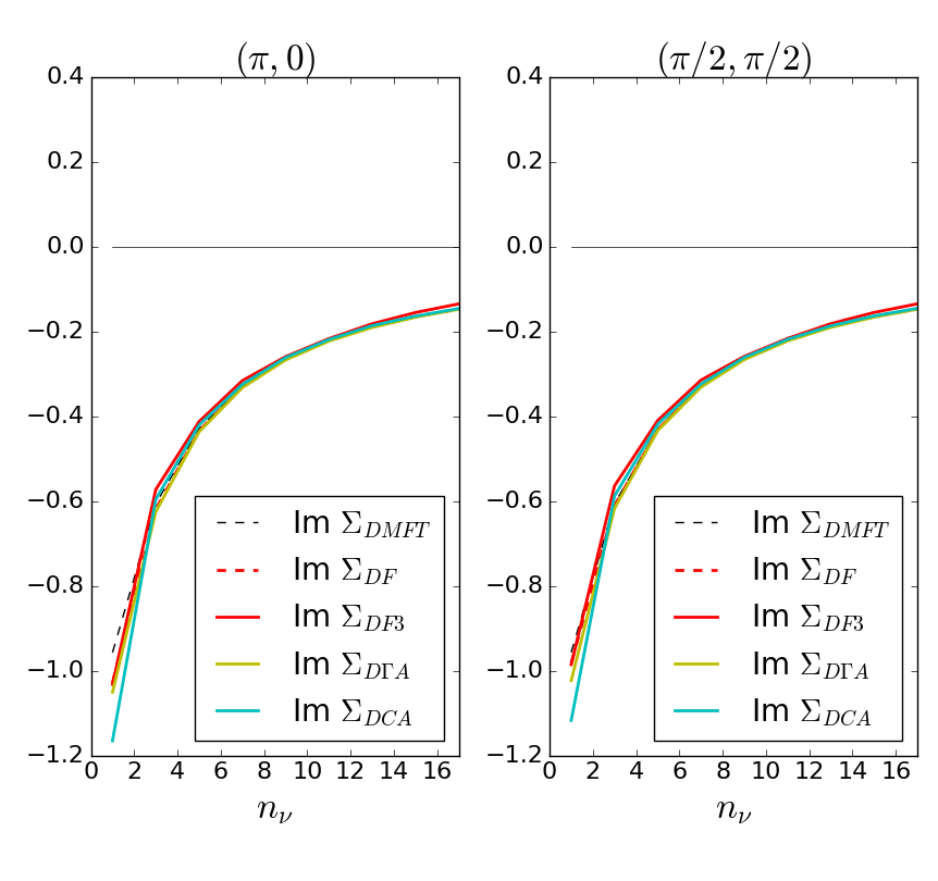
Figure 9: Comparison of the self-energy for the k-points $(\pi,0)$ and $(\pi/2,\pi/2)$ calculated from DMFT, two-particle dual fermion ($\Sigma_{DF}$), three-particle dual fermion ($\Sigma_{DF3}$), D$\Gamma$A and DCA for $72$ lattice sites for the parameters $U=2$, $\beta=8$ and $n=1$.

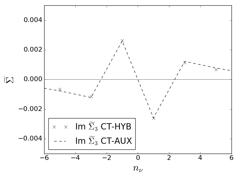
Figure 10: Comparison of $\overline{\Sigma}_{3}$ calculated from CT-AUX (dashed line) and CT-HYB (crosses) for the parameters $U=1$, $\beta=8$ and $n=1$.

V Conclusion

We have calculated local three-particle Green’s functions and vertices employing CT-QMC algorithms in the hybridization (CT-INT) and the auxiliary field expansion (CT-AUX). The structure of the vertices for a fixed entering and leaving frequency $\nu_{1}$ is found to be similar to the two-particle case. High frequency features persist in the Green’s function, and by extension, the vertex functions. Unavoidable noise in the high-frequency parts of the vertices has only weak effects when calculating three-particle self-energy corrections at small frequencies as the dual propagators within DF introduce enough damping. For larger frequencies however, the high noise level of the CT-INT vertex also reflects in a noisy self-energy, whereas the CT-AUX vertex and constructed self-energy have a low statistical error.

For different points in the parameter space of the Hubbard model, we find sizable corrections to the DF self-energy when including specific three-particle diagrams. For high enough temperatures and for the doped model, these three-particle vertex corrections are considerably smaller than the standard DF self-energy. In particular they are smaller than the two-particle DF corrections for the nodal point $(\pi/2,\pi/2)$. In this parameter regime, our calculations indicate a proper convergence of the DF theory when going to higher orders in the expansions (from the $n=2$- to the $n=3$-vertex).

For higher interaction values, this picture changes. Spin fluctuations are the dominant driving force influencing the self-energy on the two-particle level. The same kind of strong two-particle ladder contributions (the same kind of spin fluctuations) couple additionally via the three-particle vertex to an additional self-energy correction. This correction term yields an additional $\mathbf{k}$-independent contribution to the imaginary part of the self-energy, which can be interpreted as additional scattering at spin fluctuations. The considered three-particle vertex correction term also gives a $1/\nu$ asymptotic behavior which is absent in standard DF and calls for a closer investigation.

Appendix A CT-QMC measurement of the three-particle Green’s function

For completeness, this Appendix attempts to briefly summarize the construction of an estimator for the impurity three-particle Green’s function $G^{(3)}$ defined in Eq. (2). This is not a comprehensive introduction, rather it can be read as an addendum to Ref. Gull2011a, .

In the hybridization expansion (CT-HYB), we can define the interacting Green’s function by cutting hybridization lines from a given partition function configuration, i.e.:

$$G_{ij}(\tau,\tau^{\prime}) =\frac{1}{Z}\frac{\delta Z}{\delta\Delta_{ji}(\tau^{\prime},\tau)}$$

$$=\Big{\langle}\sum_{\alpha\beta}M_{\beta\alpha}\delta(\tau-\tau_{\alpha})\delta(\tau^{\prime}-\tau_{\beta}^{\prime})\delta_{ii_{\alpha}}\delta_{jj_{\beta}}\Big{\rangle}$$

$$=:\langle g_{ij}(\tau,\tau^{\prime})\rangle$$ (10)

where $\Delta(\tau,\tau^{\prime})$ is the hybridization function, $M_{\alpha\beta}^{-1}=\Delta_{i_{\alpha}j_{\beta}}(\tau_{\alpha},\tau_{\beta}^{\prime})$ is the matrix of hybridization lines, $\alpha$ and $\beta$ are indices that run over the local creation and annihilation operators, respectively, $i$ and $j$ denote spin-orbitals, and $\langle\cdot\rangle$ denote the Monte Carlo sum over the configurations of $Z$. We introduce the shorthand $g(\tau,\tau^{\prime})$ for the sum of all contributions to the Green’s function for a single configuration. Note that while the expectation value $G(\tau,\tau^{\prime})$ is time-translational invariant, this is not the case for the individual configuration $g(\tau,\tau^{\prime})$, since the inner time indices of the diagram have not yet been integrated over.

Generalizing Eq. (10) to the three-particle Green’s function, we find:

$$G_{ijklmn}(\tau_{1},\ldots,\tau_{6})= \langle g_{ij}(\tau_{1,}\tau_{2})g_{kl}(\tau_{3,}\tau_{4})g_{mn}(\tau_{5},\tau_{6})$$

$$-g_{il}(\tau_{1,}\tau_{4})g_{kj}(\tau_{3,}\tau_{2})g_{mn}(\tau_{5},\tau_{6})$$

$$-g_{in}(\tau_{1,}\tau_{6})g_{kl}(\tau_{3,}\tau_{4})g_{mj}(\tau_{5},\tau_{2})$$

$$+g_{il}(\tau_{1,}\tau_{4})g_{kn}(\tau_{3,}\tau_{6})g_{mj}(\tau_{5},\tau_{2})$$

$$+g_{in}(\tau_{1,}\tau_{6})g_{kj}(\tau_{3,}\tau_{2})g_{ml}(\tau_{5},\tau_{4})$$

$$-g_{ij}(\tau_{1,}\tau_{2})g_{kn}(\tau_{3,}\tau_{6})g_{ml}(\tau_{5},\tau_{4})\rangle\;.$$ (11)

This is nothing but the antisymmetrized sum over all possible removals of three hybridization lines, which reflects the fact that Wick’s theorem is valid for the (non-interacting) bath propagator. The frequency convention chosen in Eq. (2) translates to the following definition of the Fourier transform:

$$G_{\nu_{1}\nu\nu^{\prime}\omega}^{(3)\sigma_{1}\sigma_{2}\sigma_{3}}=\int_{0}^{\beta}d^{6}\tau\>G_{\sigma_{1}\sigma_{1}\sigma_{2}\sigma_{2}\sigma_{3}\sigma_{3}}(\tau_{1},\ldots,\tau_{6})$$

$$\qquad\qquad\times\mathrm{e}^{\mathrm{i}(\nu_{1}\tau_{1}-\nu_{1}\tau_{2}+\nu\tau_{3}-(\nu-\omega)\tau_{4}+(\nu^{\prime}-\omega)\tau_{5}-\nu^{\prime}\tau_{6})}$$ (12)

A naive implementation of Eq. (12) scales as $O(k^{6}N_{\omega}^{4})$, where $k$ is the current expansion order and $N_{\omega}$ is the number of frequencies, and is thus prohibitively expensive for even moderate $k$. A binned measurement in imaginary time, while having superior scaling $O(k^{6})$, is problematic, because $G_{ijklmn}(\tau_{1},\ldots,\tau_{6})$ is discontinuous on a set of hyperplanes $\tau_{i}=\tau_{j}$ and their intersections, which in turn translate to large binning artefacts in the Fourier transform.

It is thus advantageous split the estimator into two parts: first, we perform a Fourier transform of the single particle quantity from Eq. (10)

$$g_{ij}(\nu,\nu^{\prime}) =\int_{0}^{\beta}d\tau\,d\tau^{\prime}\,g_{ij}(\tau,\tau^{\prime})$$

$$=\sum_{\alpha\beta}M_{\beta\alpha}\exp(i\nu\tau_{\alpha}-\nu^{\prime}\tau_{\beta}^{\prime})\delta_{ii_{\alpha}}\delta_{jj_{\beta}},$$ (13)

which we can speed up by using a non-equidistant fast Fourier transform. Note again that we need to retain both frequencies, as the quantity is not time-translational invariant. Finally we perform the assembly in Eq. (11) directly in Fourier space:

$$G_{\nu_{1}\nu\nu^{\prime}\omega}^{(3)\sigma_{1}\sigma_{2}\sigma_{3}}=\langle g_{\sigma_{1}}(\nu_{1},\nu_{1})g_{\sigma_{2}}(\nu,\nu-\omega)g_{\sigma_{3}}(\nu^{\prime}-\omega,\nu^{\prime})$$

$$\qquad-g_{\sigma_{1}}(\nu_{1},\nu-\omega)g_{\sigma_{2}}(\nu,\nu_{1})g_{\sigma_{3}}(\nu^{\prime}-\omega,\nu^{\prime})\delta_{\sigma_{1}\sigma_{2}}$$

$$\qquad-g_{\sigma_{1}}(\nu_{1},\nu^{\prime})g_{\sigma_{2}}(\nu,\nu-\omega)g_{\sigma_{3}}(\nu^{\prime}-\omega,\nu_{1})\delta_{\sigma_{1}\sigma_{3}}$$

$$\qquad+g_{\sigma_{1}}(\nu_{1},\nu-\omega)g_{\sigma_{2}}(\nu,\nu^{\prime})g_{\sigma_{3}}(\nu^{\prime}-\omega,\nu_{1})\delta_{\sigma_{1}\sigma_{2}\sigma_{3}}$$

$$\qquad+g_{\sigma_{1}}(\nu_{1},\nu^{\prime})g_{\sigma_{2}}(\nu,\nu_{1})g_{\sigma_{3}}(\nu^{\prime}-\omega,\nu-\omega)\delta_{\sigma_{1}\sigma_{2}\sigma_{3}}$$

$$\qquad-g_{\sigma_{1}}(\nu_{1},\nu_{1})g_{\sigma_{2}}(\nu,\nu^{\prime})g_{\sigma_{3}}(\nu^{\prime}-\omega,\nu-\omega)\delta_{\sigma_{2}\sigma_{3}}\rangle\;.$$ (14)

Putting it all together, this reduces the scaling to $O(k^{2}N_{\omega}\log N_{\omega})+O(N_{\omega}^{4})$, which improves also on the scaling of the time binning and makes the estimator computationally feasible.

It is worth pointing out that Eq. (11), and in general any estimator for $n>1$ particles constructed in this fashion, is not valid for systems with interactions beyond density-density type and a hybridization function that is (block-)diagonal in $i$ and $j$. In such case, one would have to resort to worm sampling, which we however gauge as a formidable computational challenge in itself due to the sheer size of the worm configuration space and the size of the measured object itself. Fortunately, this is not an issue here, as we are studying the single-orbital case.

In the auxiliary field expansion (CT-AUX), one follows the same procedure of applying Eq. (14) to a Fourier transformed quantity. However, since the CT-AUX estimator is formed by adding a pair of local operators rather than cutting hybridization lines, the single particle contribution is instead given by:

$$g_{\sigma}(\nu,\nu^{\prime}) =G_{0\sigma}(\nu,\nu^{\prime})+G_{0\sigma}(\nu,\nu^{\prime})m_{\sigma}(\nu,\nu^{\prime})G_{0\sigma}(\nu,\nu^{\prime})$$ (15)

$$m_{\sigma}(\nu,\nu^{\prime}) =\sum_{\alpha\beta}M_{\alpha\beta}\exp(i\nu\tau_{\alpha}-\nu^{\prime}\tau_{\beta}^{\prime})\delta_{\sigma\sigma_{\alpha}\sigma_{\beta}},$$ (16)

where $G_{0}$ is the non-interacting Green’s functions, and $M_{\alpha\beta}$ is the matrix of auxiliary spin system. The scaling for the estimator is the same as for the CT-HYB case; however, it is evident from Eq. (15) that the CT-AUX estimator is more well-behaved at large frequencies, since the Monte Carlo signal drops as $1/\nu^{2}$ .

Appendix B Derivation of generalized Schwinger-Dyson equation

Starting from the dual fermion action Eq. (3), we can rewrite the functional-integral expression for the dual fermion propagator $\widetilde{\mathcal{G}}$ as

$$\widetilde{\mathcal{G}}_{k}=\dfrac{\int\mathcal{D}\left[\tilde{c}^{{\dagger}}\tilde{c}^{\phantom{{\dagger}}}\!\right]e^{\mathcal{S}_{dual}}\tilde{c}_{k}^{{\dagger}}\tilde{c}_{k}^{\phantom{{\dagger}}}}{\int\mathcal{D}\left[\tilde{c}^{{\dagger}}\tilde{c}^{\phantom{{\dagger}}}\!\right]e^{\mathcal{S}_{dual}}}.$$ (17)

Let us now systematically decompose $\mathcal{S}_{dual}$ into two parts $\mathcal{S}_{dual}^{k}$ and $\mathcal{S}_{dual}^{\neg k}$, where $\mathcal{S}_{dual}^{k}$ consists of all summands containing $\tilde{c}_{k}^{{\dagger}}$ and $\mathcal{S}_{dual}^{\neg k}$ of all the remaining ones (containing no $\tilde{c}_{k}^{{\dagger}}$). Since all terms in the action have an even number of Grassmann-fields, they commute and we can write

$$e^{\mathcal{S}_{dual}}=e^{\mathcal{S}_{dual}^{k}}e^{\mathcal{S}_{dual}^{\neg k}}.$$ (18)

We also know that

$$\left(\mathcal{S}_{dual}^{k}\right)^{2}=0,$$ (19)

because all of its constituting terms contain $\tilde{c}_{k}^{{\dagger}}$ (and $(\tilde{c}_{k}^{{\dagger}})^{2}=0$). Therefore, we also have

$$e^{\mathcal{S}_{dual}^{k}}=\left(1+\mathcal{S}_{dual}^{k}\right)$$ (20)

and

$$\mathcal{S}_{dual}^{k}\cdot e^{\mathcal{S}_{dual}^{k}}=\mathcal{S}_{dual}^{k}.$$ (21)

We use the relations above to rewrite Eq. (17) as

$$\widetilde{\mathcal{G}}_{k}=\dfrac{\int\mathcal{D}\left[\tilde{c}^{{\dagger}}\tilde{c}^{\phantom{{\dagger}}}\!\right]e^{\mathcal{S}_{dual}}\tilde{c}_{k}^{{\dagger}}\tilde{c}_{k}^{\phantom{{\dagger}}}}{\int\mathcal{D}\left[\tilde{c}^{{\dagger}}\tilde{c}^{\phantom{{\dagger}}}\!\right]e^{\mathcal{S}_{dual}}\mathcal{S}_{dual}^{k}}.$$ (22)

The next steps in expressing the dual self-energy are a division of both enumerator and denominator in Eq. (22) by the dual partition function $\int\mathcal{D}\left[\tilde{c}^{{\dagger}}\tilde{c}^{\phantom{{\dagger}}}\!\right]e^{\mathcal{S}_{dual}}$ and an explicit decomposition of $\mathcal{S}_{dual}^{k}$.

$$\mathcal{S}_{dual}^{k}=\left(\widetilde{\mathcal{G}}_{0,k}\right)^{-1}\tilde{c}_{k}^{{\dagger}}\tilde{c}_{k}^{\phantom{{\dagger}}}+\\ \sum_{n=2}^{\infty}\sum_{k_{1},k_{2},k_{3},...}\dfrac{1}{n!(n-1)!}F^{(n)}(k_{1},k,k_{3},k_{2},...)\tilde{c}_{k_{1}}^{\phantom{{\dagger}}}\tilde{c}_{k}^{{\dagger}}\tilde{c}_{k_{3}}^{\phantom{{\dagger}}}\tilde{c}_{k_{2}}^{{\dagger}}...$$ (23)

Here, the sum over all $k$ is gone as only the terms containing $\tilde{c}_{k}^{{\dagger}}$ are included in $\mathcal{S}_{dual}^{k}$; multiple possibilities for the summed-over indices to generate the index $k$ are taken care of by replacing one of the factors $n!$ by $(n-1)!$. We now restore normal ordering to the Grassmann-variables in $\mathcal{S}_{dual}^{k}$, yielding another factor $(-1)^{n}$ for the term containing vertices. Inserting Eq. (23) into Eq. (22), we get

$$\widetilde{\mathcal{G}}_{k}=\dfrac{\dfrac{\int\mathcal{D}\left[\tilde{c}^{{\dagger}}\tilde{c}^{\phantom{{\dagger}}}\!\right]e^{\mathcal{S}_{dual}}\tilde{c}_{k}^{{\dagger}}\tilde{c}_{k}^{\phantom{{\dagger}}}}{\int\mathcal{D}\left[\tilde{c}^{{\dagger}}\tilde{c}^{\phantom{{\dagger}}}\!\right]e^{\mathcal{S}_{dual}}}}{\dfrac{\int\mathcal{D}\left[\tilde{c}^{{\dagger}}\tilde{c}^{\phantom{{\dagger}}}\!\right]e^{\mathcal{S}_{dual}}(\widetilde{\mathcal{G}}_{0,k})^{-1}\tilde{c}_{k}^{{\dagger}}\tilde{c}_{k}^{\phantom{{\dagger}}}+\sum_{n=2}^{\infty}\sum_{k_{1},k_{2},k_{3},...}\dfrac{(-1)^{n}}{n!(n-1)!}F^{(n)}(k_{1},k,k_{3},k_{2},...)\tilde{c}_{k}^{{\dagger}}\tilde{c}_{k_{1}}^{\phantom{{\dagger}}}\tilde{c}_{k_{2}}^{{\dagger}}\tilde{c}_{k_{3}}^{\phantom{{\dagger}}}...}{\int\mathcal{D}\left[\tilde{c}^{{\dagger}}\tilde{c}^{\phantom{{\dagger}}}\!\right]e^{\mathcal{S}_{dual}}}}.$$ (24)

The enumerator by itself yields $\widetilde{\mathcal{G}}_{k}$ when performing the Grassmann-integration, while in the denominator a sum of $n$-particle dual Green’s functions multiplied by $n$-particle DMFT vertex functions and a term $\widetilde{\mathcal{G}}_{k}(\widetilde{\mathcal{G}}_{0,k})^{-1}$ appear. We divide both by the enumerator $\widetilde{\mathcal{G}}_{k}$, and end up with

$$\widetilde{\mathcal{G}}_{k}=\Bigg{(}\left(\widetilde{\mathcal{G}}_{0,k}\right)^{-1}+\sum_{n=2}^{\infty}\sum_{k_{1},k_{2},k_{3},...}\dfrac{(-1)^{n}}{n!(n-1)!}\\ F^{(n)}(k_{1},k,k_{3},k_{2},...)\widetilde{\mathcal{G}}^{(n)}(k,k_{1},k_{2},k_{3},...)/\widetilde{\mathcal{G}}_{k}\Bigg{)}^{-1},$$ (25)

where $\widetilde{\mathcal{G}}^{(n)}$ denotes the dual $n$-particle Green’s function. Employing Dyson’s equation, we recover an exact expression for the self-energy of the dual fermions

$$\widetilde{\Sigma}_{k}=-\sum_{n=2}^{\infty}\sum_{k_{1},k_{2},k_{3},...}\dfrac{(-1)^{n}}{n!(n-1)!}\\ F^{(n)}(k_{1},k,k_{3},k_{2},...)\widetilde{\mathcal{G}}^{(n)}(k,k_{1},k_{2},k_{3},...)/\widetilde{\mathcal{G}}_{k}$$ (26)

that is reminiscent of the Schwinger-Dyson equation.

References

- [1] Walter Metzner and Dieter Vollhardt. Correlated lattice fermions in dimensions. Phys. Rev. Lett., 62:324–327, Jan 1989.
- [2] E. Müller-Hartmann. Correlated fermions on a lattice in high dimensions. Zeitschrift für Physik B Condensed Matter, 74:507–512, 1988.
- [3] Antoine Georges and Gabriel Kotliar. Hubbard model in infinite dimensions. Phys. Rev. B, 45:6479–6483, Mar 1992.
- [4] A. N. Rubtsov, V. V. Savkin, and A. I. Lichtenstein. Continuous-time quantum monte carlo method for fermions. Phys. Rev. B, 72:035122, Jul 2005.
- [5] Philipp Werner, Armin Comanac, Luca de’ Medici, Matthias Troyer, and Andrew J. Millis. Continuous-time solver for quantum impurity models. Phys. Rev. Lett., 97:076405, Aug 2006.
- [6] E. Gull, P. Werner, O. Parcollet, and M. Troyer. Continuous-time auxiliary-field monte carlo for quantum impurity models. EPL (Europhysics Letters), 82(5):57003, 2008.
- [7] Emanuel Gull, Andrew J. Millis, Alexander I. Lichtenstein, Alexey N. Rubtsov, Matthias Troyer, and Philipp Werner. Continuous-time monte carlo methods for quantum impurity models. Rev. Mod. Phys., 83(2):349, May 2011.
- [8] K. Held. Dynamical vertex approximation. Dynamical Vertex Approximation [arXiv:1411.5191], 2014. in Lecture Notes ”Autumn School on Correlated Electrons. DMFT at 25: Infinite Dimensions”, Reihe Modeling and Simulation, Vol. 4, Forschungszentrum Juelich GmbH (publisher), E. Pavarini, E. Koch, D. Vollhardt, and A. I. Lichtenstein (editors) [ISBN 978-3-89336-953-9].
- [9] A. Toschi, A. A. Katanin, and K. Held. Dynamical vertex approximation; a step beyond dynamical mean-field theory. Phys Rev. B, 75:045118, 2007.
- [10] A. N. Rubtsov, M. I. Katsnelson, A. I. Lichtenstein, and A. Georges. Dual fermion approach to the two-dimensional hubbard model: Antiferromagnetic fluctuations and fermi arcs. Phys. Rev. B, 79(4):045133, 2009.
- [11] G. Rohringer, A. Toschi, H. Hafermann, K. Held, V. I. Anisimov, and A. A. Katanin. One-particle irreducible functional approach: A route to diagrammatic extensions of the dynamical mean-field theory. Phys. Rev. B, 88:115112, 2013.
- [12] G. Rohringer, H. Hafermann, A. Toschi, A. A. Katanin, A. E. Antipov, M. I. Katsnelson, A. I. Lichtenstein, A. N. Rubtsov, and K. Held. Diagrammatic routes to non-local correlations beyond dynamical mean field theory. ArXiv e-prints, 2017.
- [13] A. A. Katanin, A. Toschi, and K. Held. Comparing pertinent effects of antiferromagnetic fluctuations in the two- and three-dimensional hubbard model. Phys. Rev. B, 80:075104, Aug 2009.
- [14] A. N. Rubtsov, M. I. Katsnelson, A. I. Lichtenstein, and A. Georges. Dual fermion approach to the two-dimensional hubbard model: Antiferromagnetic fluctuations and fermi arcs. Phys. Rev. B, 79(4):045133, 2009.
- [15] C. Jung. Superperturbation theory for correlated fermions. PhD thesis, University of Hamburg, 2010.
- [16] C. Jung, A. Wilhelm, H. Hafermann, S. Brener, and A. Lichtenstein. Superperturbation theory on the real axis. Annalen der Physik, 523(8-9):706–714, 2011.
- [17] C. Taranto, S. Andergassen, J. Bauer, K. Held, A. Katanin, W. Metzner, G. Rohringer, and A. Toschi. From infinite to two dimensions through the functional renormalization group. Phys. Rev. Lett., 112:196402, May 2014.
- [18] T. Schäfer, F. Geles, D. Rost, G. Rohringer, E. Arrigoni, K. Held, N. Blümer, M. Aichhorn, and A. Toschi. Fate of the false mott-hubbard transition in two dimensions. Phys. Rev. B, 91:125109, Mar 2015.
- [19] G. Rohringer, A. Toschi, A. Katanin, and K. Held. Critical properties of the half-filled hubbard model in three dimensions. Phys. Rev. Lett., 107:256402, Dec 2011.
- [20] Andrey E. Antipov, Emanuel Gull, and Stefan Kirchner. Critical exponents of strongly correlated fermion systems from diagrammatic multiscale methods. Phys. Rev. Lett., 112:226401, Jun 2014.
- [21] D. Hirschmeier, H. Hafermann, E. Gull, A. I. Lichtenstein, and A. E. Antipov. Mechanisms of finite-temperature magnetism in the three-dimensional hubbard model. Phys. Rev. B, 92:144409, Oct 2015.
- [22] T. Schäfer, A.A. Katanin, K. Held, and A. Toschi. Quantum criticality with a twist - interplay of correlations and kohn anomalies in three dimensions. preprint, 2016.
- [23] H. Hafermann, G. Li, A. N. Rubtsov, M. I. Katsnelson, A.I. Lichtenstein, and H. Monien. Efficient perturbation theory for quantum lattice models. Phys. Rev. Lett., 102:206401, 2009.
- [24] T. Ribic, G. Rohringer, and K. Held. Local correlation functions of arbitrary order for the falicov-kimball model. Phys. Rev. B, 95:155130, 2017.
- [25] E. Gull, P. Werner, X. Wang, M. Troyer, and A. J. Millis. Local order and the gapped phase of the hubbard model: A plaquette dynamical mean-field investigation. EPL (Europhysics Letters), 84(3):37009, 2008.
- [26] Hartmut Hafermann, Kelly R. Patton, and Philipp Werner. Improved estimators for the self-energy and vertex function in hybridization-expansion continuous-time quantum monte carlo simulations. Phys. Rev. B, 85:205106, May 2012.
- [27] J. Kaufmann, P. Gunacker, and K. Held. High-frequency asymptotics of multi-orbital vertex functions in continuous-time quantum monte carlo. preprint, 2017.
- [28] A. Galler, J. Kaufmann, P. Gunacker, P. Thunström, J. M. Tomczak, and K. Held. Towards ab initio calculations with the dynamical vertex approximation. ArXiv e-prints, September 2017.
- [29] S. Brener, H. Hafermann, A. N. Rubtsov, M. I. Katsnelson, and A. I. Lichtenstein. Dual fermion approach to susceptibility of correlated lattice fermions. Phys. Rev. B, 77:195105, May 2008.
- [30] A. A. Katanin. The effect of six-point one-particle reducible local interactions in the dual fermion approach. Journal of Physics A: Mathematical and Theoretical, 46(4):045002, 2013.
- [31] The presented DF results are without self-consistency. However, for the parameters considered, imposing an inner self-energy self-consistency (not shown) leads only to minor modifications for and reduces both two- and three-particle corrections to about half their values for . A closer investigation should also include an outer self-consistency with an update of the vertex and local problem, but is beyond the scope of the present paper.
- [32] G. Rohringer and A. Toschi. Impact of nonlocal correlations over different energy scales: A dynamical vertex approximation study. Phys. Rev. B, 94:125144, Sep 2016.
- [33] T Schäfer, A Toschi, and K Held. Dynamical vertex approximation for the two-dimensional hubbard model. Journal of Magnetism and Magnetic Materials, 1506(05706), 2015.
- [34] John D. Hunter. Matplotlib: A 2d graphics environment. Computing In Science & Engineering, 9, May-Jun 2007.
- [35] Nicolaus Parragh, Alessandro Toschi, Karsten Held, and Giorgio Sangiovanni. Conserved quantities of -invariant interactions for correlated fermions and the advantages for quantum monte carlo simulations. Phys. Rev. B, 58:155158, 2012.
- [36] Markus Wallerberger et al. in preparation.
- [37] A. Gaenko, A. E. Antipov, G. Carcassi, T. Chen, X. Chen, Q. Dong, L. Gamper, J. Gukelberger, R. Igarashi, S. Iskakov, M. Könz, J. P.F. LeBlanc, R. Levy, P. N. Ma, J. E. Paki, H. Shinaoka, S. Todo, M. Troyer, and E. Gull. Updated core libraries of the alps project. Comput. Phys. Commun., 213:235–251, 4 2017.
- [38] Andrey E. Antipov, James P.F. LeBlanc, and Emanuel Gull. Opendf - an implementation of the dual fermion method for strongly correlated systems. Physics Procedia, 68:43 – 51, 2015. Proceedings of the 28th Workshop on Computer Simulation Studies in Condensed Matter Physics (CSP2015).
- [39] In the denominator, the in the expansion vanishes when integrating. The remaining term can be rewritten according to Eq. (21).