Distributed Representations of Tuples for Entity Resolution \vldbAuthorsMuhammad Ebraheem, Saravanan Thirumuruganathan, Shafiq Joty, Mourad Ouzzani, and Nan Tang \vldbDOIhttps://doi.org/10.14778/3236187.3236198
Distributed Representations of Tuples for Entity Resolution
Abstract
Despite the efforts in years in all aspects of entity resolution (ER), there is still a high demand for democratizing ER – by reducing the heavy human involvement in labeling data, performing feature engineering, tuning parameters, and defining blocking functions. With the recent advances in deep learning, in particular distributed representations of words (a.k.a. word embeddings), we present a novel ER system, called DeepER, that achieves good accuracy, high efficiency, as well as ease-of-use (i.e., much less human efforts). We use sophisticated composition methods, namely uni- and bi-directional recurrent neural networks (RNNs) with long short term memory (LSTM) hidden units, to convert each tuple to a distributed representation (i.e., a vector), which can in turn be used to effectively capture similarities between tuples. We consider both the case where pre-trained word embeddings are available as well the case where they are not; we present ways to learn and tune the distributed representations that are customized for a specific ER task under different scenarios. We propose a locality sensitive hashing (LSH) based blocking approach that takes all attributes of a tuple into consideration and produces much smaller blocks, compared with traditional methods that consider only a few attributes. We evaluate our algorithms on multiple datasets (including benchmarks, biomedical data, as well as multi-lingual data) and the extensive experimental results show that DeepER outperforms existing solutions.
1 Introduction
Entity resolution (ER) (a.k.a. record linkage), a fundamental problem in data integration, has been extensively studied for years [20], from different aspects such as declarative rules [8, 46, 50], machine learning (or probabilistic) [23, 8, 44, 13], and crowdsourcing [49, 26], to name a few, and in many domains such as health care [20], e-commerce [26], data warehouses [53], and many more.
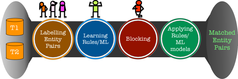
Despite the great efforts in all aspects of ER, there is still a long journey ahead in democratizing ER. Adding to the difficulty is the rapidly increasing size, number, and variety of sources of big data. Consider Figure 1 for a typical ER pipeline that consists of four main steps: (1) labeling entity pairs as either matching or non-matching pairs; (2) learning rules/ML models using the labeled data111Rules can also be hand-crafted based on domain knowledge.; (3) blocking for reducing the number of comparisons; and (4) applying the learned rules/ML models. Step (1) decides what are the matched entities. Step (2) reasons about why they match. Step (3) reduces the number of pairwise comparisons for step (4) (i.e., how), usually by expert specified blocking functions, which generate blocks such that matched entities co-exist in the same block.
Challenges. The major challenge of current solutions in democratizing ER is that each step needs human-in-the-loop. Even a “simple” step, such as step (1), which is thought to be trivial, turned out to be difficult in practice [19]. Moreover, the human resources required in each step might be different – knowing what (i.e., step (1)) is easier than telling why (i.e., step (2)) or how (i.e., step (3)). Wouldn’t it be great if we significantly reduce human cost for each step, but with a comparable if not better accuracy?
Observations. (i) In practice, step (1) is tedious because humans can only label up to several hundred (or few thousands) entity pairs and are error-prone. Intuitively, the hope to reduce this effort is to have a “prior knowledge” about what values would most likely match. (ii) Regardless of using rule-based [46, 50] or ML-based [23, 8] methods, step (2) requires experts to provide (domain-specific) similarity functions from a large pool, for example, SimMetrics (https://github.com/Simmetrics/simmetrics) has symbolic similarity functions. In addition, experts may also need to specify the thresholds. Ideally, this step needs a unified metric that can decide different cases of matched entities, from both syntactic and semantic perspectives. (iii) For step (3), a blocking function is typically defined over few attributes, e.g., and country and and gender in a table about demographic information, without a holistic view over all attributes or the semantics of the entities.
Our Methodology. We present DeepER, a system for democratizing ER that needs much less labeled data by considering prior knowledge of matched values (observation (i)), captures both syntactic and semantic similarities without feature engineering and parameter tuning (observation (ii)), and provides an automated and customizable blocking method that takes a holistic view of all attributes (observation (iii)) – all of these targets are achieved by gracefully using distributed representations, or DRs for short, (of tuples), a fundamental concept in deep learning (DL).
DRs of tuples is an extension of DRs of words (a.k.a. word embeddings) where a word is mapped to a high dimensional dense vector such that the vectors for similar words are close to each other in their semantic space. Well known methods include word2vec [40] and GloVe [43]. Word embeddings have become conventional wisdom in other fields such as NLP and have many appealing properties: (a) They are known to well capture semantic string similarities, e.g., “William” and “Bill”, and “Apple Phone” and “iPhone”. (b) Using pre-trained word embeddings (e.g., GloVe is trained on a corpus with 840 billion tokens), we can tremendously reduce the human effort of labeling matched values per dataset. (c) Due to their generality, it is possible that the same intermediate representation (such as from word2vec, GloVe, or fastText) can work for multiple datasets out-of-the-box. In contrast, traditional ER approaches require hand tuning for each dataset. (d) DR toolkits such as fastText [9] provide support for almost 294 languages allowing them, and thereby DeepER, to work seamlessly on different languages. (e) They provide a new opportunity of blocking over the vectors representing the tuples.
Contributions. In this paper, we present DeepER, a novel ER system powered by DRs of tuples, which is accurate, efficient, and easy-to-use.
1. [Distributed representations of tuples for ER.] We present two methods for effectively computing DRs of tuples by composing the DRs of all the tokens within all attribute values of a tuple. The first method is a simple averaging of the tokens’ DRs while the second uses uni- and bi-directional recurrent neural networks (RNNs) with long short term memory (LSTM) hidden units to convert each tuple to a DR (i.e., a vector).
2. [Learning/tuning distributed representations.] We introduce an end-to-end approach to tune the DRs that is customized for a specific ER task which improves the performance of DeepER (Section 3).
3. [Blocking for distributed representations.] We propose two efficient and effective blocking algorithms based on the DRs for tuples and locality sensitive hashing, which takes the semantic relatedness of all attributes into account (Section 4).
4. [Experiments.] We conducted extensive experiments (Section 5). DeepER shows superior performance compared to a state-of-the-art ER solution as well to published methods on several benchmark datasets from citations, products, and proteomics. Finally, the proposed blocking delivers outstanding results under different conditions.
2 Distributed Representations of Tuples for Entity Resolution
2.1 Entity Resolution
Let be a set of entities with tuples and attributes . Note that these entities can come from one table or multiple tables (with aligned attributes). We denote by the value of attribute on tuple . The problem of entity resolution (ER) is, given all distinct tuple pairs from where , to determine which pairs of tuples refer to the same real-world entities (a.k.a. a match).
2.2 Distributed Representations of Words
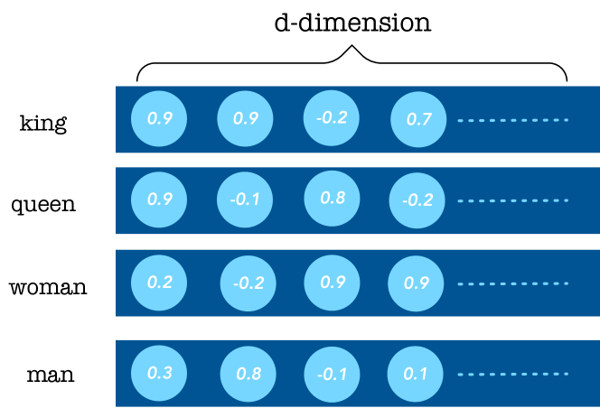
We briefly describe the concept of distributed representations (DRs) of words (please refer to [27] for more details). DRs of words (a.k.a.word embeddings) are learned from the data in such a way that semantically related words are often close to each other; i.e., the geometric relationship between words often also encode a semantic relationship between them. This embedding method seeks to map each word in a given vocabulary into a high dimensional vector with a fixed dimension (e.g., for GloVe). In other words, each word is represented as a distribution of weights (positive or negative) across these dimensions. Figure 2 shows some sample word embeddings.
Often, many of these dimensions can be independently varied. The representation is considered “distributed” since each word is represented by setting appropriate weights over multiple dimensions while each dimension of the vector contributes to the representation of many words. DRs can express an exponential number of “concepts” due to the ability to compose the activation of many dimensions [27]. In contrast, the symbolic (a.k.a. discrete) representation often leads to data sparsity and requires substantially more data to train ML models successfully [6]. Word embeddings have been successfully used to solve various tasks such as topic detection, document classification, and named entity recognition.
A number of methods have been proposed to compute the DRs of words including word2vec [40], GloVe [43], and fastText [9]. Generally speaking, these approaches attempt to capture the semantics of a word by considering its relations with neighboring words in its context. In this paper, we use GloVe, which is based on a key observation that the ratios of co-occurrence probabilities for a pair of words have some potential to encode a notion of its meaning. GloVe formalizes this observation as a log-bilinear model with a weighted least-squares objective function. This objective function has a number of appealing properties such as the vector difference between the representations for (man, woman) and (king, queen) are roughly equal.
2.3 Distributed Representations of Tuples
Similar to word embeddings, given a tuple, we need to convert it to a vector representation, such that we can measure the similarity between two tuples by computing the distance between their corresponding vectors.
Consider a tuple with attributes . Let be the vector representation of value , and be the vector representation of tuple . Also, we write the vector representation of a word . We also write as the number of dimensions of vector .
Running Example. We use the following example to illustrate our approaches. Table 2 provides a toy relation with 2 tuples and Table 2 provides word embeddings with dimensions.
| Tuple ID | : Name | : City |
|---|---|---|
| Bill Gates | Seattle | |
| William Gates | Seattle |
| Word | Distributed Representation |
|---|---|
| Bill | |
| William | |
| Gates | |
| Seattle |
Below, we describe two approaches for computing : a simple approach and a compositional approach. We then explain how we compute the similarity between two vectors.
A Simple Approach – Averaging
For each attribute value , we first break it into individual words using a standard tokenizer. For each token (word) , we look up the GloVe pre-trained dictionary and retrieve the -dimensional vector . If a word is not found in the GloVe dictionary (dubbed out-of-vocabulary scenario) or if the attribute has a NULL value, GloVe contains a special token Unk to represent such out-of-vocabulary word (we postpone the discussion of a better handling of out-of-vocabulary values to Section 3). Tokens such as IDs and some numeric values are often assigned Unk.
In our initial approach, the vector representation for an attribute value is obtained by simply averaging the vectors of its tokens in . The vector representation of tuple is the concatenation of all vectors (). That is, if each attribute value corresponds to a -dimensional vector, . Algorithm 1 describes this process.
Example 2.1.
Using our running example, and . = . The DR for and are obtained by concatenating the DRs for and .
A Compositional Approach – RNN with LSTM
We can see that the averaging based approach ignores the word order. However, it has the appealing property of being simple and very efficient to train. An alternative approach for computing is to use a compositional technique motivated by the linguistic structures (e.g., -grams, sequence, and tree) in Natural Language Processing (NLP). In this approach, instead of simple averaging, we use a neural network to semantically compose the word vectors (retrieved from GloVe) into an attribute-level vector. Considering the word order (and linguistic structure in general) could be important as many attributes contain multi-word content such as title in the citation dataset and description in the product dataset. As we shall show in our experiments, there are certain challenging datasets where being cognizant of word order improves performance. Furthermore, a tuple binds the attributes of a single entity, thus the attributes are related. Thus, an appropriate compositional approach should consider the relation between them rather than treating them separately. Different neural network architectures have been proposed to consider different types of linguistic structures, the most popular of which use a recurrent structure [36].
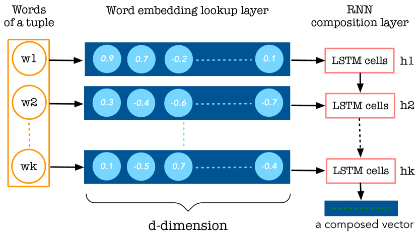
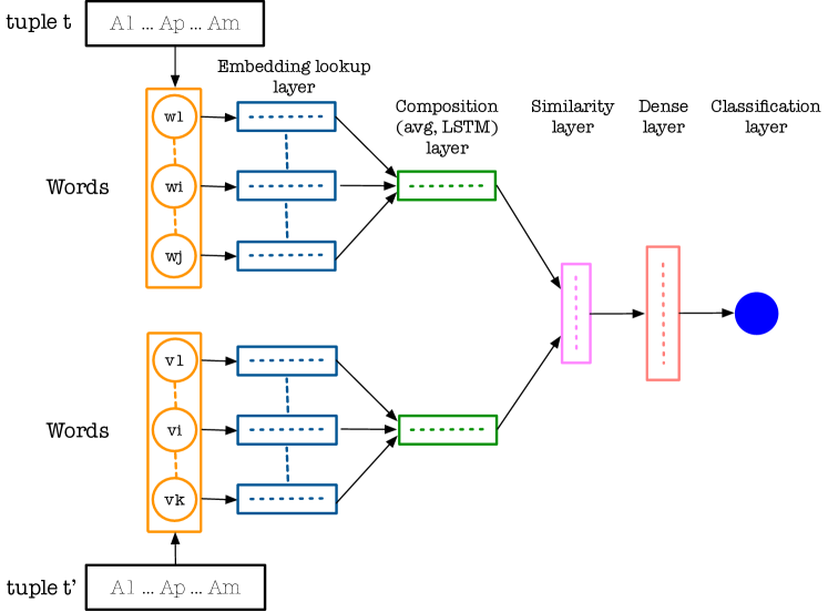
We use uni- and bi-directional recurrent neural networks (RNN) with long short term memory (LSTM) hidden units [28], a.k.a. LSTM-RNNs. As shown in Figure 3, RNNs encode a sequence of words for all attribute values (i.e., words of a tuple) into a composed vector by processing its word vectors sequentially (i.e., the word embedding lookup layer), at each time step, combining the current input word vector with the previous hidden state (i.e., the RNN composition layer). The outputted composed vector of has dimensions, where is determined by LSTM and may be different than . RNNs thus create internal states by remembering the output of the previous time step, which allows them to exhibit dynamic temporal behavior. We can interpret the hidden state at time as an intermediate representation summarizing the past. The output of the last time step thus represents the tuple. LSTM cells contain specifically designed gates to store, modify or erase information, which allow RNNs to learn long range sequential dependencies. The LSTM-RNN shown in Figure 3 is unidirectional in the sense that it encodes information from left to right.
Bidirectional RNNs [45] capture dependencies from both directions, thus provide two different views of the same sequence. For bidirectional RNNs, we use the concatenated vector as the final representation of the attribute value, where and are the encoded vectors from left to right and right to left, respectively.
Algorithm 2 gives the overall compositional process. For each word token in an attribute, we first look up its GloVe vector. Then we use a “shared”222By the term ‘shared’ we mean the parameters of the model are shared across the attributes. In other words, the LSTM-RNNs for different attributes in a table share the same parameters. LSTM-RNN to compose each attribute value in a tuple into a vector. This results in a vector of dimensions. It is important to note that the parameters of the LSTM-RNN model need to be learned on the ER task in a DL framework before it can be used to compose vectors for other off-the-shelf classifiers.
The order of attributes might not have a big effect when the number of attributes is small (such as 4 for the citations benchmark datasets). However, it might become significant when the number of attributes is large. In this case, a simple heuristic would be to ensure that semantically related attributes are close to each other. This is performed by profiling the data to find possible data dependencies. For example, if one identified that two attributes and are closely related (e.g. Country often determines Capital), then these can be ordered so that they are closer to each other.
Example 2.2.
Assume that we used a LSTM with output dimension of 2. In other words, it processes the entire tuple and produces a DR of dimension . Assume that and .
Computing Distributional Similarity
Given the DR of a pair of tuples and , the next step is to compute the similarity between their DRs and . Note that for the DRs computed by averaging, each vector has dimensions. We apply the cosine similarity on every dimensions (each dimension corresponds to one attribute), which results in a -dimensional similarity vector. For the DRs computed by LSTM, each vector has dimensions, we can use methods including subtracting (vector difference) or multiplying (hadamard product) the corresponding vector entries, resulting in a -dimensional similarity vector.
Example 2.3.
Continuing our running example, the similarity vector for tuples and for averaging is . The first component corresponds to cosine similarity of name and second the city. The distributional similarity for LSTM with vector differencing is .
2.4 ER as a Classification Problem using Distributed Representations of Tuples
ER is typically treated as a binary classification problem [23, 21, 42, 8]. Given a pair of tuples , the classifier outputs true (resp. false) to indicate that and match (resp. mismatch). The Fellegi-Sunter model [23] is a formal framework for probabilistic ER and most prior machine learning (ML) works are simple variants of this approach.
Intuitively, given two tuples and , we compute a set of similarity scores between aligned attributes based on predefined similarity functions. The vectors of known matching (resp. non-matching) tuple pairs – that are also referred to as positive (resp. negative) examples – are used to train a binary classifier (e.g., SVMs, decision trees, or random forests). The trained binary classifier can then be used to predict whether an arbitrary tuple pair is a match.
It is fairly straightforward to build a classifier for ER using the above steps. For each pair of tuples in the training dataset, we compute their DRs through either Algorithm 1 or Algorithm 2. We then compute the similarity between tuple pairs using different metrics. Given a set of positive and negative matching examples, we pass their similarity vectors to a classifier such as SVM along with their labels. Algorithm 3 provides the pseudocode.
3 Learning and Tuning
Distributed Representations
Composing DRs of words to generate DRs of tuples, as discussed in Section 2, works effectively for an ER task based on two assumptions: (i) there exist pre-trained word embeddings for most (if not all) words in the dataset; and (ii) the pre-trained word embeddings that were trained in a task agnostic manner are sufficient for the ER task. However, the above two assumptions may not hold for many real-world scenarios. The datasets that follow the above assumptions are considered as general data with full coverage (Section 3.1); the datasets that are not well covered, are considered as general data with partial coverage (Section 3.2); and the datasets that are minimally covered, are considered as specific data with minimal coverage (Section 3.3). Finally, we discuss how to tune word embeddings for an ER task (Section 3.4).
3.1 General Data with Full Coverage
Many of the benchmark datasets used in ER [18] such as Citations, Products, Restaurants, and Movies, are often generic and do not require substantial specialized knowledge. While they may be noisy and incomplete, the content is often in English and use common words. For such generic datasets, the approach that we have proposed so far – convert pairs of tuples to similarity vectors using GloVe – is often adequate. As we shall show in the experiments, we obtain competitive results for all of them.
3.2 General Data with Partial Coverage
Another case is where a significant number of words that are relevant for an ER task in a dataset are not present in the word embedding dictionary. It is well known that natural languages exhibit a Zipfian distribution with a heavy tail of infrequently used words. For computational efficiency, these “rare” words are often pruned. For example, even though GloVe was trained on a very large document corpus with 840 billion tokens and a vocabulary size of 2.2 million, it can miss many words such as from technical domains, names of people, or institutions, which would be useful for performing ER on a Citation dataset. Our approach from Section 2 replaces any word not present in the dictionary with a unique token UNK (Unknown). However, it is possible that these words are especially relevant for identifying duplicate tuples.
Vocabulary Expansion is the process of expanding the embedding dictionary to words that were not observed during training. The naive approach of adding new documents to the original corpus and re-run the whole algorithm is not always possible or feasible. For example, the popular GloVe dictionary is trained on the Common Crawl corpus, which is almost 2 TB requiring exorbitant computing resources. Given an unseen word, another simplistic approach is to take the top- words that co-occur the most with the unseen word in the ER dataset and simply average them. Another popular approach is to use character level embeddings such as fastText instead of word level embeddings or use subword information [9]. These approaches can recognize that the rare word “dendritic” is similar to “dendrites” even if it is not explicitly present in the dictionary.
While these approaches are simple and often effective, in this paper, we advocate an alternative approach inspired from [22], as described below.
Vocabulary Retrofitting. Intuitively, this approach seeks to adapt word embeddings such as GloVe by using auxiliary semantic resources such as WordNet. If there are two words that are related in WordNet, [22] seeks to refine their word embeddings to be similar. This approach is especially relevant to our scenario where our input is a tuple with explicit attribute structure and has relational interpretations.
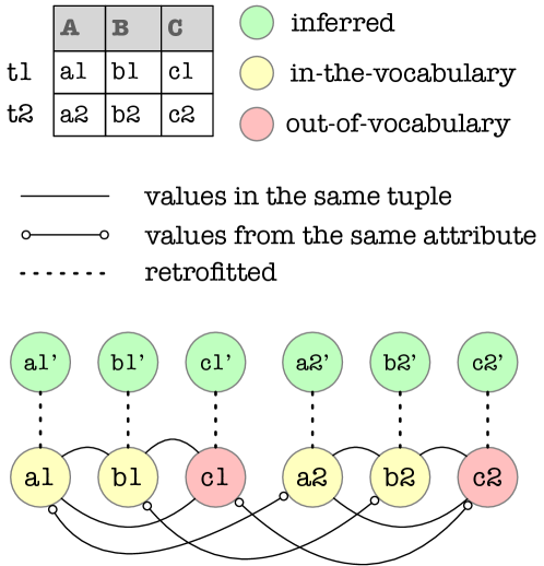
Let be the set of words from the ER dataset. Let be the set of words with no word embeddings. We begin by creating an undirected graph with one vertex for each word in . Two vertices are connected if they co-occur in some tuple. One can also define other additional edge semantics such as an edge connecting two vertices if they occur in the same attribute and so on. For vertex , we assign its word embedding from the dictionary. For vertex , we assign its initial value as the average of of its most frequent co-occurring words. We then create a set of new vertices for each word and connect it to its corresponding vertex from . These vertices correspond to the retrofitted word embeddings that will be learned through probabilistic inference. We set the objective function such that we learn the word embeddings for each vertex such that they are both closer to its counterpart in and also closer to its other neighboring vertices. Figure 4 shows an example.
This approach has a number of appealing properties. First, this is an efficient mechanism to learn the word embeddings of unknown words such as IDs. Second, it provides an elegant mechanism to “tune” the word embeddings that is in sync with the ER dataset. For example, if two words do not co-occur a lot in Common Crawl (such as SIGMOD and Stonebraker) but does in our dataset, this approach tunes the embeddings appropriately. Finally, it allows one to encode a diverse array of options to define relatedness (such as present in the same attribute or tuple) that is more generic than the simple co-occurrence idea used by GloVe.
3.3 Specific Data with Minimal Coverage
Another common scenario occurs when one performs ER on datasets with specialized information. Examples include performing ER on scientific articles for specialized fields or in data that is specific to an organization. In this case, the attributes often contain esoteric words that are not present in GloVe dictionary. What is worse, it might not know that two terms such as p53 and cancer are related. If most of the words are not present in the dictionary, then approaches such as retrofitting might be applicable. This problem could be exacerbated if the ER dataset belongs to complex domains such as Genomics. Finding if two tuples describe the same protein might not be possible with GloVe or word2vec.
We use one of the following approaches to handle such scenarios:
(1) Unsupervised Representation from Datasets. If the two datasets that are to be merged are large enough (typically in the order of millions of tuples), they might contain enough patterns to automatically learn word embeddings from them. One could pool all the tuples from both datasets and train GloVe/word2vec on them by treating each tuple as a document.
(2) Unsupervised Learning from related Corpus. If the datasets are not large enough, then one can find another surrogate resource to learn word embeddings. GloVe and word2vec learned the word embeddings by training on a large corpus such as Common Crawl and Google News respectively. If one can find an analogous vast corpus of domain information in the form of unstructured data such as documents, it could be used to learn the word embeddings for this specialized dataset. For example, while word embeddings from GloVe might not know that p53 and cancer are related, the word embeddings trained from PubMed articles would be able to. Similarly, one could learn word embeddings from the enterprise’s document repository for ER on data in the same organization.
(3) Customized Word Embeddings. In some cases, it is possible that direct application of GloVe or word2vec does not solve the problem. For example, when given a huge amount of training they might not find if, for example, two strings encode the same protein. In such cases, one has to check if there exist prior methods for learning word embeddings for the task of interest. For example, there exist prior work on word embeddings for proteins and genes from sequences of amino acids and DNA respectively [3].
Of course, the worst case scenario is a specialized database where no auxiliary resources are available to automatically learn the representation for key concepts. In this scenario, any machine learning approach is doomed to fail unless one provides hand crafted features or a substantially large number of training examples that are sufficient for learning representations using deep learning.
3.4 Tuning Word Embeddings for an ER Task
Recall that word embeddings such as GloVe/word2vec are learned in an unsupervised task-agnostic manner so that they can be used for arbitrary tasks. If the corpus used to train them is large and representative enough, the learned word embeddings can be used in a turn-key manner for ER tasks. While unsupervised pre-training on a large corpus does give the DL model better generalization, in many cases the learned representations often lack task-specific knowledge. One can achieve the best of both worlds by fine-tuning the pre-trained word representations to achieve better accuracy. In fact, this paradigm of unsupervised pre-training followed by supervised fine-tuning often beats methods that are based on only supervision [15].
Our proposed approach can be easily extended for this purpose. Let us now consider our deep neural network in Figure 5. We train this network using Stochastic Gradient Descent (SGD) based learning algorithms, where gradients (errors) are obtained via backpropagation. In other words, errors in the output layer (i.e., the classification layer) are backpropagated through the hidden layers using the chain rule of derivatives. The parameters of the hidden layers are slightly altered such that when the model accuracy improves. For learning or fine-tuning the embeddings, we allow these errors to be backpropagated all the way till the word embedding layer. In contrast, our approach from Section 2 can only tune parameters up to the composition layer. Allowing error to be back propagated to the embedding layer allows one additional level of freedom to tinker model parameters. Instead of limiting ourselves to how the attributes are composed or how similarity is computed, we can also modify the word embeddings themselves (if necessary).
One common issue with backpropagation through a deep neural network (i.e., neural networks with many hidden layers such as RNNs) is that as the errors get propagated, they may soon become very small (a.k.a. gradient vanishing problem) or very large (a.k.a. gradient exploding problem) that can lead to undesired values in weight matrices, causing the training to fail [7]. We did not observe such problems in our end-to-end training with simple averaging compositional method, and the gates in LSTM cells automatically tackle these issues to some extent [28].
4 Blocking for Distributed Representations
Efficient ER systems avoid comparing all possible pairs of tuples ( for one table of for two tables) through the use of blocking [4, 12]. Blocking identifies groups of tuples (called blocks) such that the search for duplicates need to be done only within these blocks, thus greatly reducing the search space. While blocking often substantially reduces the number of comparisons, it may also miss some duplicates that fall in two different blocks.
4.1 New Opportunities for Blocking
We observe that blocking is very related to the classical problem of approximate nearest neighbor (ANN) search in a similarity space, which has been extensively studied (see [51]). Locality sensitive hashing (LSH) [29] is a popular probabilistic technique for finding ANNs in a high dimensional space. In the blocking context, the more similar input vectors are, the higher the probability that they both will be put in the same block. While we are not the first to propose LSH for blocking or automated tuning for blocking (see Section 6), we are the first to propose a series of truly turn-key algorithms for blocking.
Challenges in Traditional Blocking Approaches
(i) Identifying good blocking rules often requires the assistance of domain experts.
(ii) Blocking rules often consider few (e.g., 2-3) attributes which could result in comparing tuples that agree on those attributes but have very different values on other attributes.
(iii) Prior blocking methods often do not take semantic similarity between tuples into consideration.
(iv) It is usually hard to tune the blocking strategy to control the recall and/or the size of the blocks.
We can readily see that LSH for blocking over DRs of tuples obviates many of these issues. First, we free the domain experts from providing a blocking function. Instead the combination of LSH and DRs transforms the problem of blocking into finding tuples in a high dimensional similarity space. Note that a DR encodes semantic similarity into the mix and that LSH considers the entire tuple for computing similarity. The extensive amount of theoretical work on LSH (see Section 4.5) can be used to both tune and provide rigorous theoretical guarantees on the performance.
4.2 LSH Primer
Definition 4.1.
The smaller the value of (), the better the search performance. For many popular distance measures such as cosine, Euclidean, and Jaccard, there exists an algorithm for the -nearest neighbor problem that requires space (where is the dimensionality of ), query time, and invocations of hash functions. In practice, LSH requires linear space and time [25, 51].
Implementing LSH. Given a table , LSH seeks to index all the tuples in a hash table that is composed of multiple buckets each of which is identified by a unique hash code. Given a tuple , the bucket in which it is placed by a (single) hash function is denoted as - which is often a binary value. If two tuples and are very similar, then with high probability. Typically, one uses hash functions , , to encode a single tuple . We represent as a dimensional binary vector which in turn is represented by its hash code . Since the usage of hash functions reduces the likelihood that similar items will obtain the same ( dimensional) hash code, we repeat the above process times - . Intuitively, we build hash tables where each bucket in a hash table is represented by a hash code of size . Each tuple is then hashed into different hash tables where its hash codes are . For example, if and , every tuple is represented as a 10-dimensional binary vector that is stored in 2 different hash tables.
Hash Families for Cosine Distance. Cosine similarity provides an effective method for measuring semantic similarity between two DRs [43]. Since the DRs can have both positive and negative real numbers, the cosine similarity varies between and . The family of hash functions for cosine is obtained using the random hyperplane method. Intuitively, we choose a random hyperplane through the origin that is defined by a normal unit vector . This defines a hash function with two buckets where if and if where “” denotes the dot product between vectors. Since we require hash functions , we randomly pick hyperplanes and each tuple is hashed with them to obtain a dimensional hash code. This process is then repeated for all hash tables.
4.3 LSH-based Blocking
We begin by generating hash codes for each of the hash tables using the random hyperplane method. The set of hash functions is analogous to a single blocking rule. The dimensional binary hash code is equivalent to an identifier to a distinct block where falls into. Each hash table performs “blocking” using a different blocking rule.
We index the DR of every tuple in each of the hash tables. LSH guarantees that similar tuples get the same hash code (and hence fall into the same block) with high probability. Then, we consider each of the blocks for every hash table and invoke the classifier over the distinct pairs of tuples found in them. Algorithm 4 provides the corresponding pseudocode.
Example 4.2.
For simplicity, let us only hash the DR for attribute of tuples and . Let and . Let the hash functions be , , and . Recall that and . If you do a dot product of with each of the ’s, you get . The corresponding output for is . Note that the LSH hash code is obtained by thresholding the values such that positive values get and negative values . So the hash code of both these tuples is .
Algorithm 4 is a fairly straightforward adaptation of LSH to ER. As we shall see in the experiments, it works well empirically. However, the number of times a classifier would be invoked can be as much as where is the number of hash tables, is the size of the largest block in any hash table and is the maximum number of non-empty blocks in any hash table. While the traditional LSH based approach is often efficient and effective, one can achieve improved performance with some additional domain knowledge. We next describe a sophisticated approach to reduce the impact of and .
4.4 Multi-Probe LSH for Blocking
Recall that by increasing , we ensure that the probability of dissimilar tuples falling into the same block is reduced. By increasing , we ensure that similar tuples fall into the same block in at least one of the hash tables. Hence while increasing ensures that we will not miss a true duplicate pair, it is achieved at the additional cost of making extraneous comparisons between non-duplicate tuples. We wish to come up with a LSH based approach that achieves two objectives: (a) reduce the number of unnecessary comparisons and (b) reduce the number of hash tables without seriously affecting recall.
Reducing Unnecessary Comparisons. Intuitively, we expect duplicate tuples to have a high similarity with each other and thereby more likely to be “near” each other. Hence, even if a block has a large number of tuples, it is not necessary to compare all pairs of tuples. Instead, given a tuple , we retrieve the top- nearest neighbors of and invoke the classifier between and these nearest neighbors. This is achieved by collating all the tuples that fall into the same block as in each of the hash tables. We then compute the similarity between and each of the candidates and return the top- tuples. If the block is large with tuples, then we only require classifier invocations instead of . We can see that by choosing , we can achieve considerable reduction in classifier invocations.
Reducing . Naively decreasing the number of hash tables can decrease the recall as a pair of duplicate tuples might fall into different blocks. The key idea is to augment a traditional LSH scheme with a carefully designed probing sequence that looks for multiple buckets (of the same hash table) that could contain similar tuples with high probability. This approach is called multi-probe LSH [37]. Consider a tuple and another very similar tuple . It is possible that and do not fall into the same bucket (especially if is large). However, due to the design of LSH, we would expect to fall into a “close by” bucket whose hash code is very similar to the bucket in which fell. Multi-probe leverages this observation by perturbing in a systematic manner and looking at all buckets in which the perturbed fell into. By carefully designing the perturbation process one can consider the buckets that have the highest probability of containing similar tuples. For example, a multi-probe of size 1 will consider all buckets whose hash codes have a hamming distance of 1 and so on. It has been shown that this approach often requires substantially less number of hash tables (as much as 20x) than a traditional approach [37]. Algorithm 5 provides the pseudocode of this approach.
4.5 Tuning LSH Parameters for Blocking
In contrast to traditional blocking rules that are often heuristics, the hash functions in LSH allow us to provide rigorous theoretical guarantees. While the list of LSH guarantees is beyond the scope of this paper (see [47] for details), we highlight two major ones.
Parameter Tuning for Recall. We can control the false positive and negative values (and thereby recall) by varying the values of and , such as by setting the values that get the best results for the tuples in the training dataset. We can obtain a fixed approximation ratio of by setting [51],
| (1) |
Parameter Tuning for Occupancy. LSH also allows us to control the occupancy - the expected number of tuples in any given block. This can be achieved by varying the size of the number of hash functions in every hash table. Informally, if one uses multiple hash functions, we would expect very similar items to be stored in the same blocks but at the expense of low occupancy and a large number of blocks. On the other hand, a smaller number of hash functions results in less similar tuples being put in the same block. Intuitively, if we use only one hash function, this results in 2 buckets - one for and . Since the hyperplane for the hash function is chosen randomly, we would expect each bucket to have an occupancy around 50% for all but most of the skewed data distributions. One can reduce the occupancy rate by increasing the number of hash functions. Alternatively, one can also use sophisticated methods such as [16] to achieve guaranteed limits.
| Dataset | #Tuples | #Matches | #Attr |
| Walmart-Amazon‡[18] | 2,554 - 22,074 | 1,154 | 17 |
| Amazon-Google‡ [1] | 1,363 - 3,226 | 1,300 | 5 |
| DBLP-ACM∗ [1] | 2,616 - 2,294 | 2,224 | 4 |
| DBLP-Scholar∗ [1] | 2,616 - 64,263 | 5,347 | 4 |
| DBLP-Citeseer∗ [18] | 1,823,978-2,512,927 | 558,787 | 4 |
| Fodors-Zagat∗ [2] | 533 - 331 | 112 | 7 |
| Dataset | Magellan | DeepER | Published |
| Prod-WA | 82.99 | 88.06 | 89.3 [26] (Crowd) |
| Prod-AG | 87.68 | 96.029 | 62.2 [33] (ML) |
| Pub-DA | 97.6 | 98.6 | N/A |
| Pub-DS | 98.84 | 97.67 | 92.1 [26] (Crowd) |
| Pub-DC | 96.4 | 99.1 | 95.2 [17] (Crowd) |
| Rest-FZ | 100 | 100 | 96.5 [26] (Crowd) |
5 Experimental Results
5.1 Experimental Setup
Hardware and Platform. All our experiments were performed on a Core i7 6700HQ Skylake chip, with four cores running eight threads at speeds of up to 3.5GHz, along with 16GB of DDR4 RAM and the GTX 980M, complete with 8GB of DDR5 RAM. We used Torch [14] and Keras [11], a deep learning framework, to train and test our models.
Datasets. We conducted extensive experiments over different datasets covering diverse domains such as citations, e-commerce, and proteomics. Table 4 provides some statistics of these datasets. All are popular benchmark datasets and have been extensively evaluated by prior ER work using both ML and non-ML based approaches. We partition our datasets into two categories: “easy” and “challenging”. The former consists of datasets that are mostly structured and often have less noise in terms of typos and missing information. On the “easy” datasets most of the best existing ER approaches routinely exceed an F-score of . The challenging datasets often have unstructured attributes (such as product description) which are also noisy. On the “challenging” datasets that we study, both ML and rule based methods have struggled to achieve high F measures, with values between and being the norm. What these two categories have in common is that they require extensive effort from domain experts for cleaning, feature engineering and blocking to achieve good results. As we shall show later, our approach exceeds best existing results on all the datasets with minimal expert effort.
DeepER Setup. Our experimental setup was an adaptation of prior ER evaluations methods [32, 33, 46] to handle DRs. For example, [32] used an arbitrary threshold (such as 0.1) on Jaccard similarity of trigram to eliminate tuple pairs that are clearly non-matches. We make two changes to this procedure. First, we use Cosine similarity to compute similarity between tuple pairs as it is more appropriate for DRs [40, 43]. Second, instead of picking an arbitrary threshold, we set it to the minimum similarity of matched tuple pairs in the training dataset. We obtain the negative examples (non duplicates) by picking one tuple from the positive example and randomly picking another tuple from the relation that is not its match. For example, if is a duplicate, we pick a pair as a negative example such that is not a duplicate already given in the training data and has cosine similarity with below the above computed threshold. This approach is chosen to verify the robustness of our models against near matches. For each of the datasets, we performed -fold cross validation with K=5. We report the average of the F-measure values obtained across all the folds. We observed that in all cases, the standard deviation of the F-measure values was below 1%.
DeepER Architecture. Since our objective is to highlight the turn-key aspect of DeepER, we choose the simplest possible architecture. We use GloVe[43] as our DR. Figure 5 shows the architecture of DeepER. We used Adam for optimizing the DL model that were trained for 20 epochs with a batch size of 16. The learning rate was set to 0.01 and a regularization of 1e-3. For RNN-LSTM composition, we used a single RNN layer where the memory dimension for LSTM is 150. The dimension of the similarity layer is 50. When end-to-end learning is enabled, the embeddings update rate was set to 0.01.
Each tuple is represented as a dimensional vector where is the number of attributes with being the dimension of DRs. For each attribute, we apply a standard tokenizer and average the DR obtained from GloVe (as against more sophisticated approaches such as Bi-LSTM). Given a pair of tuples, the compositional similarity is computed as the Cosine similarity of the corresponding attributes resulting in a dimensional similarity vector. As mentioned above, we used -fold validation with a duplicate to non-duplicate ratio of 1:100 that is comparable to the ratio used by the competing approaches. This is to ensure fair comparison. Note that the non-duplicates are sampled automatically from the positive examples. This is achieved by selecting other tuple pairs that have a low cosine similarity with the duplicate being perturbed. This approach was inspired from [34] where they demonstrate that an informative negative example is one that is far from the positive example. Quoting from their example, “truck” is selected over “dog” as the negative example for “cat”. We also do not tune the DR for the ER task. Even with this restricted setup, DeepER is competitive with existing approaches.
5.2 Comparison with Existing Methods
We first compare the performance of DeepER with the best reported results from non-learning, learning and crowd based approaches in [33, 26, 17]. Table 4 shows that the simple DeepER architecture has better performance, except for one dataset, namely Prod-WA, where a crowd-based approach does slightly better.
Performing ER on a large dataset requires a number of design choices from the expert such as feature engineering, selection of appropriate similarity functions and thresholds, parameter tuning for ML models, selection of appropriate blocking functions, and so on. Hence, it is incredibly hard to take any of the existing approaches and apply it as-is on a new dataset. A key advantage of DeepER is the ability to dramatically reduce this effort. In order to highlight this feature, we evaluated DeepER against Magellan [31] that also has a end-to-end EM pipeline. We would like to emphasize that both DeepER and Magellan share the dream of making the EM process as frictionless as possible. While Magellan uses a series of sophisticated heuristics internally, DeepER leverages DRs as a foundational technique. It is very easy to incorporate features from DeepER and Magellan to each other. For example, one can augment Magellan’s automatically derived similarity based features to DeepER while Magellan can readily use the blocking of DeepER and so on. Table 4 compares the performance of DeepER and Magellan using their default settings. Specifically, we adapted the end-to-end EM workflow for Magellan [38]. We can see that DeepER beats Magellan on two datasets, while performing slightly worst in one datasets. Both systems delivered perfect results in the rather simple Fodors-Zagat dataset.
Evaluating DeepER for Other Domains. In order to show that our approach can be readily applied to other domains, we consider the problem of determining duplicates in a nucleotide database. We assumed that we were provided with an appropriate dictionary for biomedical embeddings. We evaluated our model on a large benchmark dataset [10] consisting of 21 most heavily studied organisms in molecular biology. Our method was able to beat ML models with hand-crafted approach in 11 of these cases while it was within a F1-score of 5 for the remaining. Overall, our approach achieved an F1-measure of 87.4 for the automatic curation benchmark where the state-of-the-art is 83.9. This shows that our approach can be readily applied to other domains given the availability of effective embeddings.
5.3 Understanding DeepER Performance
We next investigate how each of the enhancements to the basic DeepER architecture impacts its performance. For this subsection, we use a positive to negative ratio of 1:4. This is different from the ratio we used when compared to competing approaches as this turned to be best for DeepER.
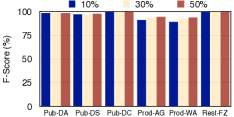
Varying the Size of Training Data. Figure 8 shows the results of varying the amount of training data. DeepER is robust enough to be competitive with other approaches with as little as 10% of training data. Note that 10% translates to as little as 11 examples to label in the case of Rest-FZ and to 543 in the case of Pub-DS. As expected, our method improves its excellent results with larger training data. This is due to two key aspects: (a) the ability of DeepER to leverage/transfer the semantic similarity learned by DRs for ER and (b) a DL architecture that is customized for ER. Please refer to [5, 27, 54] for additional details about the beneficial impact of effective representation/transfer learning and well designed DL architectures.
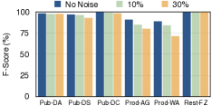
Impact of Incorrect Labels. Most of the prior work on ER assumes that the training data is perfect. However, this assumption might not always hold in practice. Given the increasing popularity of crowdsourcing for obtaining training data, it is likely that some of the labels for matching and non-matching pairs are incorrect. We investigate the impact of incorrect labels in this experiment. For a fixed set of training data (10%), we vary the fraction of labels that are marked incorrectly. Figure 8 shows the results. While the F-measure reduces with larger fraction of incorrect labels, the experiments also show that our approach is very robust. The average drop in F-measure values compared to the perfect labeling case across all datasets at 10% noise is just 2.6 with a standard deviation of 2.6. At 30% the average drop is 8% with a standard deviation of 7%. We can also see that at 10% noising, our approach is still competitive with state-of-the-art approaches.
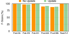
Dynamic vs Static Word Embeddings. In this set of experiments, we evaluated the effect of updating (or fine-tuning) the initial word embeddings obtained from GloVe as part of training the model. In other words, we evaluated if tuning the DR for ER tasks improves the performance of our model. Figure 8 shows the results. The results matched our intuition that for the “challenging” datasets, updating the word embeddings in an end-to-end learning framework helped boost the results a little, whilst for the “easy” ones, it had either a small negative effect or no effect at all. Thus, we advise that in general, it is better to use the end-to-end framework.
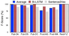
Varying Composition. In this set of experiments, we vary the compositional method we use to combine the individual word embeddings into a single representative vector for the tuple/attribute. In addition to word averaging and LSTM, we added a method based on Sentence2Vec [35] and that is tuned using our end-to-end learning methods (Section 3.4), for completeness. Figure 9 shows that for the “easy” datasets, simple word averaging work usually better than recurrent compositional models (LSTM or BiLSTM). This flips for the “challenging” datasets where sophisticated compositional approaches perform slightly better. This is especially noticeable for Prod-AG. Understanding and automatically recommending the appropriate architecture for a given dataset is a key focus of our future research. In order to use the more complex compositional methods (LSTM or BiLSTM) one has to pay the price of its longer training times, one also has to tune its additional hyperparameters. However, even the simple averaging compositional technique is competitive with prior approaches on all datasets. We also observe that both methods are superior to Sentence2Vec with a slight exception on the Prod-AG dataset where it is superior to Average.
Varying Word Embedding Dictionaries. Here, we study the impact of the dictionary used for DRs. GloVe has two major dictionaries : one trained on Common Crawl web corpus (840B tokens, 2.2M words) and one on Wikipedia (6B tokens, 400K words). We used the vocabulary retrofitting to handle words not present in the dictionary. Table 5 shows the result of the experiments. As expected, there is a steep drop in F1 score when trained on a smaller dictionary. The larger the corpus used for training the word embeddings, the better they are identifying semantic relationships.
| Dataset | GloVe | GloVe-Wiki |
| Pub-DA | 98.6 | 82.1 |
| Pub-DS | 97.67 | 77.8 |
| Pub-DC | 99.1 | 79.2 |
| Prod-WA | 88.06 | 77.4 |
| Prod-AG | 96.029 | 87.2 |
| Rest-FZ | 100 | 91.2 |
Varying Word Embedding Models. We conducted experiments on three popular models, GloVe, Word2Vec, and FastText, which were trained on a corpus with 840B tokens, 100B tokens and 600B tokens, respectively. The number of words identified are 2.2M, 3M, and 1M, respectively. Note that for fairness of comparison, we only considered word embeddings in FastText even though it also allows character embeddings. We used the vocabulary retrofitting to handle words not present in the dictionary. Table 6 shows the results of the experiments. In general, there are only minor variations between the different approaches.
| Dataset | GloVe | Word2Vec | FastText |
| Pub-DA | 98.6 | 97.9 | 98.2 |
| Pub-DS | 97.6 | 96.9 | 97.2 |
| Pub-DC | 99.1 | 99 | 99 |
| Prod-WA | 88.06 | 86.1 | 88.89 |
| Prod-AG | 96.03 | 95.1 | 95.7 |
| Rest-FZ | 100 | 100 | 100 |
Multi-Lingual Datasets. We now show an auxiliary benefit of using a DR-based approach. We took three datasets that were originally in English and translated them to Spanish. We then used the DRs for Spanish and repeated our approach. Table 7 shows that while there is a reduction in F1-score, our approaches can seamlessly work on multi-lingual datasets. Since we used “Google translate”, we had to limit how much we could translate. However, we expect to see similar results with the other datasets.
| Dataset | English | Spanish |
|---|---|---|
| Prod-AG | 96.029 | 89.1 |
| Rest-FZ | 100 | 92.6 |
| Pub-DS | 97.67 | 88.1 |
5.4 Evaluating LSH-based Blocking
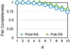
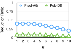
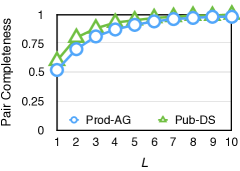
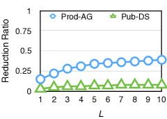
In this subsection, we evaluate the performance of our LSH based blocking approach. Our approach allows us to vary (the size of the hash code) and (the number of hash tables) in order to achieve a tunable performance. Recall that one can use Equation 1 to derive and based on the task requirements. Suppose we wish that similar tuples should fall into same bucket with probability and dissimilar tuples should fall into the same bucket with probability . Suppose that we index the DBLP dataset of Pub-DS. Then based on Equation 1, we need a LSH with and .
In our first set of experiments, we verify that the behavior of blocking is synchronous with the theoretical expectations. We evaluate the performance of blocking based on two metrics widely used in prior research [4, 12, 39]. The first metric, efficiency or reduction ratio (RR), is the ratio of the number of tuple pairs compared by our approach to the number of all possible pairs in . In other words, a smaller value indicates a higher reduction in the number of comparisons made. The second metric, recall or pair completeness (PC), is the ratio of the number of true duplicates compared by our approach against the total number of duplicates in . A higher value for PC means that our approach places the duplicate tuple pairs in the same block.
Figures 10(a)-10(d) show the results of our experiments. As is increased, the value of PC decreases. This is due to the fact that for a fixed , increasing reduces the likelihood that two similar tuples will be placed in the same block which in turn reduces the number of duplicates that falls into the same block. However, for a fixed , increasing dramatically decreases the RR. This is to be expected as a larger value of increases the number of LSH buckets into which tuples can be assigned to.
A complementary behavior can be observed when we fix and vary . When increases, PC also increases. This is to be expected as the probability that two similar tuples being assigned to the same bucket increases when more than one hash table is involved. In other words, even if a true duplicate does not fall into the same bucket in one hash table, it can fall into the same bucket in other hash tables. However, increasing has a negative impact on RR as some false positive tuple pairs can fall into the same bucket in at least one hash table thereby increasing the value of RR.
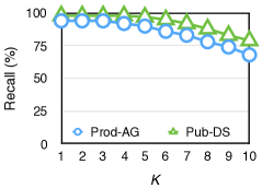
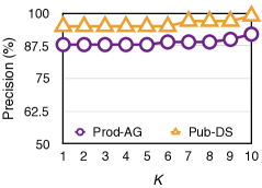
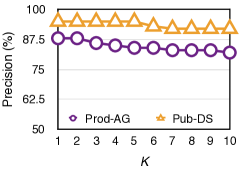
Evaluating DeepER End-to-End. We next evaluate the performance of DeepER by combining both the blocker and the matcher. The results are shown in Figure 11. First, we study how precision and recall are impacted by varying for a fixed . The recall decreases with increased as more and more duplicates are not put in the same block which results in DeepER missing them. The precision increases mildly with increasing as an increasing number of spurious non-duplicates are no longer being compared. For example, when , almost half of all possible pairs are classified by DeepER, which reduces the precision with potential false positives. However, when , only a quarter of all possible pairs are classified, resulting in mild increase of precision. The reason for the mild increase is that the classifier of DeepER is relatively robust and achieved high precision even for low value of .
Figures 10 c-d study the impact of varying for a fixed on precision and recall. As expected, the recall increases with higher as almost all the true duplicates are put in the same block and end up being classified as such by DeepER. Since DeepER is quite accurate, this results in increased recall. The precision declines mildly with increasing . The reason is that more and more non-duplicates are put in the same block resulting in potential false positives. Once again, the impact is mild as the classifier is relatively robust.
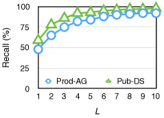
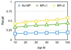
Evaluating Multi-Probe LSH. We evaluate Algorithm 5 using Multi-probe and comparing a tuple only with top- most similar tuples instead of all tuples in a block. Figure 12 shows the result for Pub-AG. We vary the number of multi-probes and pick the top-N most similar tuples to be classified. We measure the recall of this approach for and an extreme case with a single hash table where . We wish to highlight two trends. First, even using a single multi-probe sequence can dramatically increases the recall. This supports our claim that one can increase recall using a small number of hash tables by using multi-probe LSH. Second, increasing the size of does not dramatically increase the recall. This is due to the fact that duplicate tuples have high similarity between their corresponding distributed representations. Our top- based approach would be preferable to reduce the number of classifier invocations when the block size is much higher than 10.
6 Related Work
Entity Resolution. A good overview of ER can be found in surveys such as [21, 42]. Prior work can be categorized as based on (a) declarative rules, (b) ML and (c) expert or crowd based. Declarative rules, such as DNF which specify rules for matching tuples, are easily interpretable [46] but often requires a domain expert. Most of the ML approaches are variants of the classical Fellegi-Sunter model [23]. Popular approaches include SVM [8], active learning [44], clustering [13]. Recently, ER using crowdsourcing has become popular [49, 26]. While there exist some work for learning similarity functions and thresholds [8, 50], ER often requires substantial involvement of the expert.
There has been extensive work on building EM systems. [31] provides a comprehensive survey of the current EM systems. Most of the prior works often do not cover the entire EM pipeline, require extensive interaction with experts and are not turn-key systems. The key objective of DeepER is the same as Magellan [31]. We propose a end-to-end EM system based on DR that minimizes the burden on the experts. Our techniques are modular enough and can be easily incorporated into any of the existing systems.
There has been extensive interest in applying DL in data cleaning [48]. A recent work that extends DeepER [41] explored the design space of ER using DRs. The authors introduce four different choices for the attribute summarization process, namely, SIF, RNN, Attention, and Hybrid. The first two methods are similar to our AVG and LSTM-RNN methods. Attention uses decomposable attention for attribute summarization and vector concatenation to perform attribute comparison. Hybrid uses a bidirectional RNN with decomposable attention for attribute summarization and a vector concatenation and element-wise absolute difference during attribute comparison. While this work shares some similarities with DeepER, there are two notable differences. We present solutions for the practical situations where for dealing with data with partial or minimal coverage. We also propose efficient and effective blocking solutions.
Blocking. Blocking has been extensively studied as a way to scale ER systems and a good overview can be found in surveys such as [4, 12]. Common approaches include key-based blocking that partitions tuples into blocks based on their values on certain attributes and rule-based blocking where a decision rule determines which block a tuple falls into. There has been limited work on simplifying this process by either learning blocking schemes such as [39] or tuning the blocking [30]. In contrast, our work automates the blocking process by requiring minimal input from the domain expert.
Some recent works used LSH for blocking. [47] uses MinHashing where tuples with high Jaccard similarity are likely to be assigned to the same block. [52] improves it by proposing a MinHashing with semantic similarity based on concept hierarchy to assign conceptually similar tuples to the same block. [24] proposed a clustering based method to satisfy size constraints with upper and lower size thresholds for blocks for performance and privacy reasons.
7 Final Remarks
In this paper, we introduced DeepER, a DL-based approach for ER. Our fundamental contribution is the identification of the concept of DRs as a key building block for designing effective ER classifiers. We also propose algorithms to transform a tuple to a DR, building DR-aware classifiers and an efficient blocking strategy based on LSH. Our extensive experiments show that our approach is promising and already achieves or surpasses the state-of-the-art on multiple benchmark datasets. We believe that DL is a powerful tool that has applications in databases beyond ER and it is our hope that our ideas be extended to build practical and effective ER systems.
There are several avenues for improving DeepER. First, understand and automatically recommend the appropriate DL architecture for a given dataset, especially complex ones. Another line of work is to design a hybrid system that leverages both automatic features, such as DRs, and manual features, such as a similarity metric for IDs. Finally, we will also need to address the cases where the data is dirty.
References
- [1] Benchmark datasets for entity resolution. https://dbs.uni-leipzig.de/en/research/projects/object_matching/fever/benchmark_datasets_for_entity_resolution.
- [2] Duplicate detection, record linkage, and identity uncertainty: Datasets. http://www.cs.utexas.edu/users/ml/riddle/data.html.
- [3] E. Asgari and M. R. Mofrad. Continuous distributed representation of biological sequences for deep proteomics and genomics. PloS one, 10(11):e0141287, 2015.
- [4] R. Baxter, P. Christen, and T. Churches. A comparison of fast blocking methods for record linkage. In SIGKDD Workshop on Data Cleaning, Record Linkage, and Object Consolidation, 2003.
- [5] Y. Bengio, A. Courville, and P. Vincent. Representation learning: A review and new perspectives. IEEE transactions on pattern analysis and machine intelligence, 35(8):1798–1828, 2013.
- [6] Y. Bengio, R. Ducharme, P. Vincent, and C. Janvin. A neural probabilistic language model. JMLR, 2003.
- [7] Y. Bengio, P. Simard, and P. Frasconi. Learning long-term dependencies with gradient descent is difficult. Trans. Neur. Netw., 5(2):157–166, Mar. 1994.
- [8] M. Bilenko and R. J. Mooney. Adaptive duplicate detection using learnable string similarity measures. In KDD, 2003.
- [9] P. Bojanowski, E. Grave, A. Joulin, and T. Mikolov. Enriching word vectors with subword information. arXiv preprint arXiv:1607.04606, 2016.
- [10] Q. Chen, J. Zobel, and K. Verspoor. Benchmarks for measurement of duplicate detection methods in nucleotide databases. Database, 2016.
- [11] F. Chollet. Deep learning with Python. Manning Publications, 2018.
- [12] P. Christen. A survey of indexing techniques for scalable record linkage and deduplication. TKDE, 2012.
- [13] W. W. Cohen and J. Richman. Learning to match and cluster large high-dimensional data sets for data integration. In KDD, 2002.
- [14] R. Collobert, K. Kavukcuoglu, and C. Farabet. Torch7: A matlab-like environment for machine learning. In BigLearn, NIPS Workshop, 2011.
- [15] R. Collobert, J. Weston, L. Bottou, M. Karlen, K. Kavukcuoglu, and P. Kuksa. Natural language processing (almost) from scratch. JMLR, 2011.
- [16] M. Covell and S. Baluja. Lsh banding for large-scale retrieval with memory and recall constraints. In ICASSP, 2009.
- [17] S. Das, P. S. G. C., A. Doan, J. F. Naughton, G. Krishnan, R. Deep, E. Arcaute, V. Raghavendra, and Y. Park. Falcon: Scaling up hands-off crowdsourced entity matching to build cloud services. In SIGMOD, pages 1431–1446, 2017.
- [18] S. Das, A. Doan, P. S. G. C., C. Gokhale, and P. Konda. The magellan data repository. https://sites.google.com/site/anhaidgroup/projects/data.
- [19] A. Doan, A. Ardalan, J. R. Ballard, S. Das, Y. Govind, P. Konda, H. Li, S. Mudgal, E. Paulson, P. S. G. C., and H. Zhang. Human-in-the-loop challenges for entity matching: A midterm report. In HILDA@SIGMOD, 2017.
- [20] H. L. Dunn. Record linkage. American Journal of Public Health, 36 (12), 1946.
- [21] A. K. Elmagarmid, P. G. Ipeirotis, and V. S. Verykios. Duplicate record detection: A survey. TKDE, 19(1), 2007.
- [22] M. Faruqui, J. Dodge, S. K. Jauhar, C. Dyer, E. Hovy, and N. A. Smith. Retrofitting word vectors to semantic lexicons. arXiv preprint arXiv:1411.4166, 2014.
- [23] I. Fellegi and A. Sunter. A theory for record linkage. Journal of the American Statistical Association, 64 (328), 1969.
- [24] J. Fisher, P. Christen, Q. Wang, and E. Rahm. A clustering-based framework to control block sizes for entity resolution. In KDD, 2015.
- [25] A. Gionis, P. Indyk, R. Motwani, et al. Similarity search in high dimensions via hashing. In PVLDB, volume 99, pages 518–529, 1999.
- [26] C. Gokhale, S. Das, A. Doan, J. F. Naughton, N. Rampalli, J. W. Shavlik, and X. Zhu. Corleone: hands-off crowdsourcing for entity matching. In SIGMOD, pages 601–612, 2014.
- [27] I. Goodfellow, Y. Bengio, and A. Courville. Deep Learning. MIT Press, 2016. http://www.deeplearningbook.org.
- [28] S. Hochreiter and J. Schmidhuber. Long short-term memory. Neural computation, 9(8):1735–1780, 1997.
- [29] P. Indyk and R. Motwani. Approximate nearest neighbors: Towards removing the curse of dimensionality. In Proceedings of the Thirtieth Annual ACM Symposium on the Theory of Computing, Dallas, Texas, USA, May 23-26, 1998, pages 604–613, 1998.
- [30] B. Kenig and A. Gal. Mfiblocks: An effective blocking algorithm for entity resolution. Information Systems, 2013.
- [31] P. Konda, S. Das, P. Suganthan GC, A. Doan, A. Ardalan, J. R. Ballard, H. Li, F. Panahi, H. Zhang, J. Naughton, et al. Magellan: Toward building entity matching management systems. PVLDB, 9(13):1581–1584, 2016.
- [32] H. Köpcke and E. Rahm. Training selection for tuning entity matching. In QDB/MUD, 2008.
- [33] H. Köpcke, A. Thor, and E. Rahm. Evaluation of entity resolution approaches on real-world match problems. PVLDB, 3(1):484–493, 2010.
- [34] A. Lazaridou, G. Dinu, and M. Baroni. Hubness and pollution: Delving into cross-space mapping for zero-shot learning. In Proceedings of the 53rd Annual Meeting of the Association for Computational Linguistics and the 7th International Joint Conference on Natural Language Processing (Volume 1: Long Papers), volume 1, pages 270–280, 2015.
- [35] Q. Le and T. Mikolov. Distributed representations of sentences and documents. In ICML, 2014.
- [36] J. Li, T. Luong, D. Jurafsky, and E. Hovy. When are tree structures necessary for deep learning of representations? In EMNLP, 2015.
- [37] Q. Lv, W. Josephson, Z. Wang, M. Charikar, and K. Li. Multi-probe lsh: efficient indexing for high-dimensional similarity search. In PVLDB, pages 950–961, 2007.
- [38] Magellan. End-to-end em workflows, 2017.
- [39] M. Michelson and C. A. Knoblock. Learning blocking schemes for record linkage. In AAAI, pages 440–445, 2006.
- [40] T. Mikolov, I. Sutskever, K. Chen, G. S. Corrado, and J. Dean. Distributed representations of words and phrases and their compositionality. In NIPS, 2013.
- [41] S. Mudgal, H. Li, T. Rekatsinas, A. Doan, Y. Park, G. Krishnan, R. Deep, E. Arcaute, and V. Raghavendra. Deep learning for entity matching: A design space exploration. In SIGMOD, 2018.
- [42] F. Naumann and M. Herschel. An introduction to duplicate detection. Synthesis Lectures on Data Management, 2(1):1–87, 2010.
- [43] J. Pennington, R. Socher, and C. D. Manning. Glove: Global vectors for word representation. In EMNLP, 2014.
- [44] S. Sarawagi and A. Bhamidipaty. Interactive deduplication using active learning. In KDD, 2002.
- [45] M. Schuster and K. K. Paliwal. Bidirectional recurrent neural networks. IEEE TSP, 1997.
- [46] R. Singh, V. Meduri, A. K. Elmagarmid, S. Madden, P. Papotti, J. Quiané-Ruiz, A. Solar-Lezama, and N. Tang. Synthesizing entity matching rules by examples. PVLDB, 11(2):189–202, 2017.
- [47] R. C. Steorts, S. L. Ventura, M. Sadinle, and S. E. Fienberg. A comparison of blocking methods for record linkage. In PSD, 2014.
- [48] S. Thirumuruganathan, N. Tang, and M. Ouzzani. Data curation with deep learning : Towards self driving data curation. arXiv preprint arXiv:1803.01384, 2018.
- [49] J. Wang, T. Kraska, M. J. Franklin, and J. Feng. Crowder: Crowdsourcing entity resolution. PVLDB, 5(11):1483–1494, 2012.
- [50] J. Wang, G. Li, J. X. Yu, and J. Feng. Entity matching: How similar is similar. PVLDB, 4(10):622–633, 2011.
- [51] J. Wang, H. T. Shen, J. Song, and J. Ji. Hashing for similarity search: A survey. arXiv preprint arXiv:1408.2927, 2014.
- [52] Q. Wang, M. Cui, and H. Liang. Semantic-aware blocking for entity resolution. TKDE, 2016.
- [53] W. E. Winkler. Data quality in data warehouses. In Encyclopedia of Data Warehousing and Mining, Second Edition (4 Volumes), pages 550–555. 2009.
- [54] J. Yosinski, J. Clune, Y. Bengio, and H. Lipson. How transferable are features in deep neural networks? In Advances in neural information processing systems, pages 3320–3328, 2014.