One-loop perturbative coupling of $A$ and $A_{\star}$ through the chiral overlap operator

Abstract

Recently, Grabowska and Kaplan constructed a four-dimensional lattice formulation of chiral gauge theories on the basis of the chiral overlap operator. At least in the tree-level approximation, the left-handed fermion is coupled only to the original gauge field $A$, while the right-handed one is coupled only to the gauge field $A_{\star}$, a deformation of $A$ by the gradient flow with infinite flow time. In this paper, we study the fermion one-loop effective action in their formulation. We show that the continuum limit of this effective action contains local interaction terms between $A$ and $A_{\star}$, even if the anomaly cancellation condition is met. These non-vanishing terms would lead an undesired perturbative spectrum in the formulation.

1 Introduction and discussion

Recently, Grabowska and Kaplan proposed a four-dimensional lattice formulation of chiral gauge theories Grabowska:2016bis . This formulation is based on the so-called overlap operator, which can be obtained from their five-dimensional domain-wall formulation Grabowska:2015qpk by the traditional way Neuberger:1997bg ; Vranas:1997da ; Kikukawa:1999sy . In this formulation, along the fifth dimension, the original gauge field $A$ is deformed by the gradient flow Narayanan:2006rf ; Luscher:2009eq ; Luscher:2010iy ; Luscher:2011bx for infinite flow time. Since the gradient flow preserves the gauge covariance, this formulation is manifestly gauge invariant, even if the anomaly cancellation condition is not met. Although there is a subtlety associated with the topological charge Grabowska:2015qpk ; Grabowska:2016bis ; Okumura:2016dsr ; Makino:2016auf ; Hamada:2017tny , the smeared gauge field after the infinite-flow time, $A_{\star}$, only to which the right-handed (invisible) fermion would be coupled, can be basically considered as pure gauge (see Appendix A). Then one would regard their setup as the system of the left-handed fermion interacting with the gauge field $A$; this picture was however confirmed only in the tree-level approximation Grabowska:2016bis . It is thus a crucial problem whether radiative corrections induce the physical coupling of the right-handed fermion or not.

First, let us see the tree-level decoupling between the physical and invisible sectors. So far, only when the transition of the flowed gauge field along the fifth dimension is abrupt, the four-dimensional lattice Dirac operator has been obtained as an explicit form; this is referred to as the chiral overlap operator $\hat{\mathcal{D}}_{\chi}$. The operator $\hat{\mathcal{D}}_{\chi}$ is given by Grabowska:2016bis

$$a\hat{\mathcal{D}}_{\chi}=1+\gamma_{5}\left[1-(1-\epsilon_{\star})\frac{1}{\epsilon\epsilon_{\star}+1}(1-\epsilon)\right],$$ (1)

where $a$ is the lattice spacing, and $\epsilon$ ($\epsilon_{\star}$) is the sign function Neuberger:1997fp ; Neuberger:1998wv

$$\epsilon\equiv\frac{H_{w}(A)}{\sqrt{H_{w}(A)^{2}}}\qquad\left(\epsilon_{\star}\equiv\frac{H_{w}(A_{\star})}{\sqrt{H_{w}(A_{\star})^{2}}}\right),$$ (2)

of the Hermitian Wilson Dirac operator

$$H_{w}=\gamma_{5}\left[\frac{1}{2}\gamma_{\mu}(\nabla_{\mu}+\nabla_{\mu}^{*})-\frac{1}{2}a\nabla_{\mu}\nabla_{\mu}^{*}-m\right],$$ (3)

where $m$ is the parameter of the domain-wall height, and $\gamma_{\mu}$ is the Dirac matrix. In this expression, $\nabla_{\mu}$ is the forward gauge covariant lattice derivative and $\nabla_{\mu}^{*}$ is the backward one. With the assumption of abruptness, this Dirac operator depends on the two gauge fields, $A$ and $A_{\star}$. In the classical continuum limit Grabowska:2016bis ,

$$am\hat{\mathcal{D}}_{\chi}\stackrel{{\scriptstyle a\to 0}}{{\to}}\gamma_{\mu}D_{\mu}(A)P_{-}+\gamma_{\mu}D_{\mu}(A_{\star})P_{+},$$ (4)

where $D_{\mu}(A)$ ($D_{\mu}(A_{\star})$) is the covariant derivative defined with respect to $A$ ($A_{\star}$), and $P_{\pm}=(1\pm\gamma_{5})/2$ are the chirality projection operators. Therefore, the coupling between the gauge fields, $A$ and $A_{\star}$, is not produced in the tree-level approximation.

Let us study how the decoupling between $A$ and $A_{\star}$ is modified under radiative corrections. The fermion one-loop effective action is defined by

$$\ln\mathcal{Z}[A,A_{\star}]\equiv\ln\int\prod_{x}\left[d\psi(x)d\bar{\psi}(x)\right]\exp\left[-a^{4}\sum_{x}\bar{\psi}(x)\hat{\mathcal{D}}_{\chi}\psi(x)\right],$$ (5)

where $A$ and $A_{\star}$ are regarded as independent non-dynamical variables. To investigate the (de)coupling, two infinitesimal variations $\delta$ and $\delta_{\star}$ are introduced such that $\delta$ acts only on $A$ but not on $A_{\star}$,

$$\delta A\neq 0,\qquad\delta A_{\star}\equiv 0,$$ (6)

and $\delta_{\star}$ acts in an opposite way,

$$\delta_{\star}A\equiv 0,\qquad\delta_{\star}A_{\star}\neq 0.$$ (7)

Then, we will find that in the continuum limit a double variation of the effective action is given as

$$\delta\delta_{\star}\ln\mathcal{Z}[A,A_{\star}]=-\int d^{4}x\,\mathcal{L}(A,A_{\star};\delta A,\delta_{\star}A_{\star}),$$ (8)

where $\mathcal{L}(A,A_{\star};\delta A,\delta_{\star}A_{\star})$ is a local polynomial of its arguments and their spacetime derivatives.

To find a possible implication of Eq. (8), we take gauge variations as $\delta$ and $\delta_{\star}$:

$$\delta^{\omega}A_{\mu}(x) \equiv\partial_{\mu}\omega(x)+[A_{\mu}(x),\omega(x)], \delta^{\omega}A_{\star\mu}(x) =0,$$ (9)

$$\delta_{\star}^{\omega}A_{\star\mu}(x) \equiv\partial_{\mu}\omega(x)+[A_{\star\mu}(x),\omega(x)], \delta_{\star}^{\omega}A_{\mu}(x) =0.$$ (10)

Since, as a property of the gradient flow, the two gauge fields $A$ and $A_{\star}$ transform in the same way under the gauge transformation, the gauge invariance of the effective action implies

$$(\delta^{\omega}+\delta_{\star}^{\omega})\ln\mathcal{Z}[A,A_{\star}]=0\Rightarrow\delta(\delta^{\omega}+\delta_{\star}^{\omega})\ln\mathcal{Z}[A,A_{\star}]=0.$$ (11)

Therefore, using Eq. (8), we can obtain

$$\delta\delta^{\omega}\mathcal{Z}[A,A_{\star}]=-\delta\delta_{\star}^{\omega}\mathcal{Z}[A,A_{\star}]=\int d^{4}x\,\mathcal{L}(A,A_{\star};\delta A,\delta_{\star}^{\omega}A_{\star}).$$ (12)

Now, let us assume that $A_{\star}$ becomes pure gauge under the gradient flow with infinite flow time (see Appendix A):

$$A_{\star}=g^{-1}dg.$$ (13)

Then the gauge transformation $A^{g^{-1}}$ makes $A_{\star}=0$, where

$$A^{g}=g^{-1}(d+A)g.$$ (14)

That is, we can impose the $A_{\star}=0$ gauge on Eq. (12)

$$\delta\delta^{\omega}\ln\mathcal{Z}[A,0]=\int d^{4}x\,\mathcal{L}(A,A_{\star}=0;\delta A,\delta_{\star}^{\omega}A_{\star}|_{A_{\star}=0}).$$ (15)

We will see below that the right-hand side does not vanish even if the anomaly cancellation condition is met.

It will be shown in the next section that $\ln\mathcal{Z}[A,0]$ has the term

$$\ln\mathcal{Z}[A,0]=\int d^{4}x\,\frac{f_{0}}{2a^{2}}\operatorname{tr}A_{\mu}A_{\mu}+\cdots,$$ (16)

thus the mass term $\operatorname{tr}A_{\mu}A_{\mu}$ is produced in the one-loop level. The propagator of the gauge potential in this $A_{\star}=0$ thus has the structure,

$$\left\langle A_{\mu}^{a}(x)A_{\nu}^{a}(y)\right\rangle=g_{0}^{2}\,\delta^{ab}\int\frac{d^{4}p}{(2\pi)^{4}}\,e^{ip(x-y)}\left(\delta_{\mu\nu}-\frac{p_{\mu}p_{\nu}}{p^{2}}\right)\frac{1}{p^{2}+m_{A}^{2}+\cdots},$$ (17)

where we have defined the mass parameter $m_{A}$ as

$$m_{A}^{2}=g_{0}^{2}\frac{f_{0}}{2a^{2}}.$$ (18)

Therefore, the perturbative spectrum is modified in a weird way; this would not be what we want to obtain for chiral gauge theories. Since these effects in the one-loop effective action (16) should be removed by local counterterms, the formulation of Grabowska and Kaplan will be undesirable as a non-perturbative formulation of chiral gauge theories. Then their formulation with the abrupt transition should be improved in some possible way.

2 Explicit forms of $\mathcal{L}$ and $\delta^{\omega}\ln\mathcal{Z}$

In this section, we show the results of the continuum limit of $\mathcal{L}(A,A_{\star};\delta A,\delta_{\star}A_{\star})$. In what follows, we use the variables

$$C_{\mu} \equiv A_{\star\mu}-A_{\mu},$$ (19)

$$\bar{A}_{\mu} \equiv\frac{1}{2}(A_{\mu}+A_{\star\mu}),$$ (20)

$$\bar{D}_{\mu} \equiv\partial_{\mu}+[\bar{A}_{\mu},\cdot],$$ (21)

and the field strength

$$\bar{F}_{\mu\nu} =\partial_{\mu}\bar{A}_{\nu}-\partial_{\nu}\bar{A}_{\mu}+[\bar{A}_{\mu},\bar{A}_{\nu}].$$ (22)

We also define the following lattice integrals:

$$f_{0}(am) \equiv\int_{p}\left(-\frac{1}{4t}-\frac{s_{\rho}^{2}}{4t}-\frac{cc_{\rho}}{4t}\right),$$ (23)

$$f_{1}(am) \equiv\int_{p}\left(\frac{1}{64t^{2}}-\frac{c_{\rho}c_{\sigma}}{128t}+\frac{s_{\rho}^{2}s_{\sigma}^{2}}{32t^{2}}\right),$$ (24)

$$f_{2}(am) \equiv\int_{p}\left(-\frac{c_{\rho}c_{\sigma}}{32t}+\frac{7s_{\rho}^{2}s_{\sigma}^{2}}{64t^{2}}+\frac{cs_{\rho}^{2}c_{\sigma}}{32t^{2}}+\frac{c^{2}c_{\rho}c_{\sigma}}{64t^{2}}\right),$$ (25)

$$f_{3}(am) \equiv\int_{p}\left(-\frac{c_{\rho}c_{\sigma}}{32t}+\frac{3s_{\rho}^{2}s_{\sigma}^{2}}{32t^{2}}-\frac{s_{\rho}^{2}}{32t^{2}}-\frac{cc_{\rho}}{32t^{2}}\right),$$ (26)

$$f_{4}(am) \equiv\int_{p}\left(\frac{1}{96t}+\frac{s_{\rho}^{2}}{96t}+\frac{cc_{\rho}}{96t}+\frac{1}{16t^{2}}\right),$$ (27)

$$f_{5}(am) \equiv\int_{p}\left(\frac{1}{16t}+\frac{c_{\rho}c_{\sigma}}{32t}+\frac{7}{32t^{2}}-\frac{c^{2}}{32t^{2}}+\frac{cc_{\rho}}{16t^{2}}+\frac{s_{\rho}^{2}}{32t^{2}}\right),$$ (28)

where

$$s_{\rho} \equiv\sin p_{\rho}, c_{\rho} \equiv\cos p_{\rho},$$ (29)

$$c \equiv\sum_{\mu}(c_{\mu}-1)+am, t \equiv\sum_{\mu}s_{\mu}^{2}+c^{2},$$ (30)

$$\int_{p} \equiv\int_{-\pi}^{\pi}\frac{d^{4}p}{(2\pi)^{4}}.$$ (31)

$f_{i}(am)$ ($i=0,\dots,5$) as the function of $am$ are plotted in Figs. 2–6.

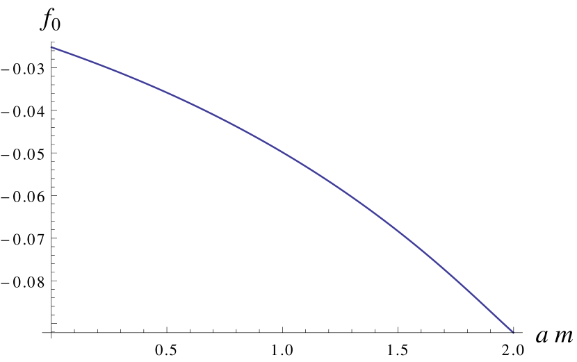
Figure 1: $f_{0}(am)$

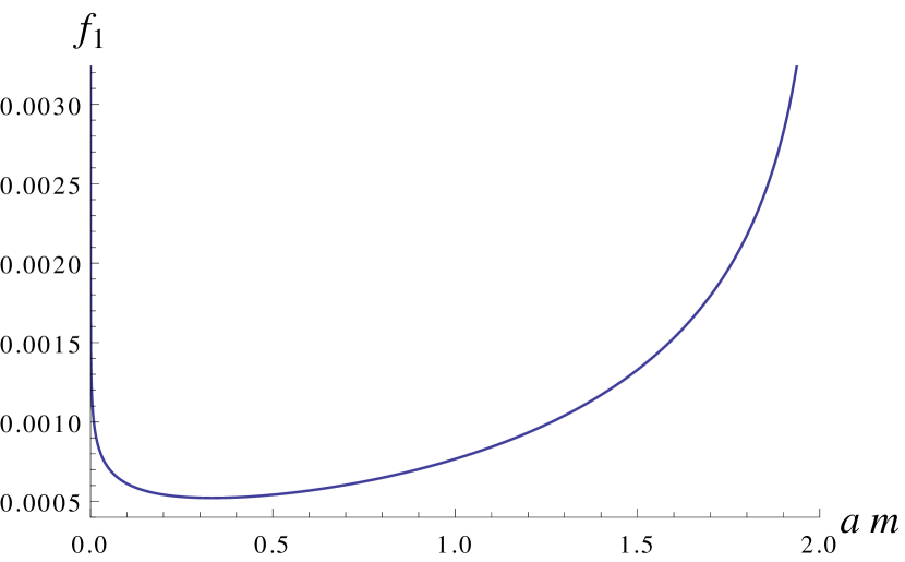
Figure 2: $f_{1}(am)$

Figure 3: $f_{2}(am)$

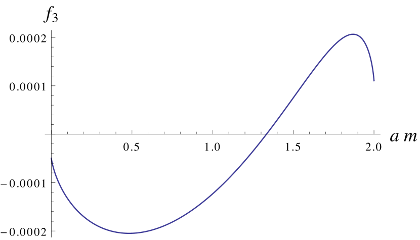
Figure 4: $f_{3}(am)$

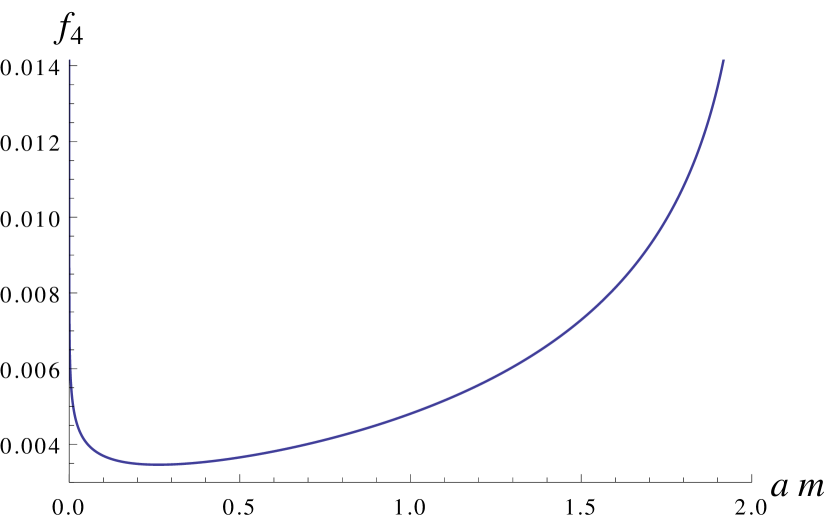
Figure 5: $f_{4}(am)$

Figure 6: $f_{5}(am)$

The local functional $\mathcal{L}$ has three parts, according to the parity and Lorentz symmetry: (i) the parity-odd and Lorentz-preserving part, (ii) the parity-even and Lorentz-preserving part, and (iii) the parity-even and Lorentz-violating part. First, the parity-odd part of $\mathcal{L}$ is given by

$$\left.\mathcal{L}(A,A_{\star};\delta A,\delta_{\star}A_{\star})\right|_{\text{parity-odd}}$$

$$=-\frac{1}{32\pi^{2}}\epsilon_{\mu\nu\rho\sigma}\Biggl{[}\left(\bar{F}_{\mu\nu}+\frac{1}{12}[C_{\mu},C_{\nu}]\right)\{\delta A_{\rho},\delta_{\star}A_{\star\sigma}\}$$

$$\qquad\qquad\qquad\qquad{}-\frac{1}{3}C_{\mu}\left(\{\delta A_{\nu},\bar{D}_{\rho}\delta_{\star}A_{\star\sigma}\}+\{\delta_{\star}A_{\star\nu},\bar{D}_{\rho}\delta A_{\sigma}\}\right)\Biggr{]},$$ (32)

where and in what follows the symbol $\operatorname{tr}$ is assumed to be omitted. This part is proportional to the gauge anomaly coefficient; thus this vanishes if the anomaly cancellation condition is met. Second, we have the parity-even and Lorentz-preserving part of $\mathcal{L}$,

$$\left.\mathcal{L}(A,A_{\star};\delta A,\delta_{\star}A_{\star})\right|_{\text{parity-even, Lorentz-preserving}}$$

$$=\frac{f_{0}}{a^{2}}\delta A_{\mu}\delta_{\star}A_{\star\mu}$$

$$\qquad{}+\left(-\frac{3f_{1}}{2}+\frac{f_{2}}{2}-\frac{f_{3}}{2}\right)[(\bar{D}_{\mu}\delta A_{\mu})C_{\nu}\delta_{\star}A_{\star\nu}-C_{\mu}\delta A_{\mu}(\bar{D}_{\nu}\delta_{\star}A_{\star\nu})]$$

$$\qquad{}-\left(\frac{f_{1}}{2}+\frac{f_{2}}{2}-\frac{3f_{3}}{2}\right)[C_{\mu}(\bar{D}_{\nu}\delta A_{\mu})\delta_{\star}A_{\star\nu}-\delta A_{\mu}C_{\nu}(\bar{D}_{\mu}\delta_{\star}A_{\star\nu})]$$

$$\qquad{}-\left(\frac{f_{1}}{2}+\frac{f_{2}}{2}-\frac{3f_{3}}{2}\right)[C_{\nu}\delta A_{\mu}(\bar{D}_{\mu}\delta_{\star}A_{\star\nu})-(\bar{D}_{\nu}\delta A_{\mu})C_{\mu}\delta_{\star}A_{\star\nu}]$$

$$\qquad{}+\left(-\frac{7f_{1}}{2}+\frac{f_{2}}{2}+\frac{f_{3}}{2}\right)[(\bar{D}_{\mu}C_{\mu})\delta A_{\nu}\delta_{\star}A_{\star\nu}-\delta A_{\nu}(\bar{D}_{\mu}C_{\mu})\delta_{\star}A_{\star\nu}]$$

$$\qquad{}-\left(\frac{3f_{1}}{2}-\frac{f_{2}}{2}+\frac{f_{3}}{2}\right)[\delta A_{\mu}C_{\mu}(\bar{D}_{\nu}\delta_{\star}A_{\star\nu})-C_{\nu}(\bar{D}_{\mu}\delta A_{\mu})\delta_{\star}A_{\star\nu}]$$

$$\qquad{}+\left(13f_{1}-3f_{2}-3f_{3}\right)(\bar{D}_{\mu}\delta A_{\mu})(\bar{D}_{\nu}\delta_{\star}A_{\star\nu})$$

$$\qquad{}+\left(9f_{1}-3f_{2}-f_{3}\right)(\bar{D}_{\mu}\delta A_{\nu})(\bar{D}_{\mu}\delta_{\star}A_{\star\nu})$$

$$\qquad{}+\left(-19f_{1}+5f_{2}+5f_{3}\right)(\bar{D}_{\nu}\delta A_{\mu})(\bar{D}_{\mu}\delta_{\star}A_{\star\nu})$$

$$\qquad{}+\left(\frac{11f_{1}}{6}-\frac{f_{2}}{6}-\frac{7f_{3}}{6}\right)C_{\mu}\delta A_{\nu}C_{\mu}\delta_{\star}A_{\star\nu}$$

$$\qquad{}+\left(-\frac{13f_{1}}{6}+\frac{11f_{2}}{6}-\frac{7f_{3}}{6}\right)(C_{\mu}\delta A_{\mu}C_{\nu}\delta_{\star}A_{\star\nu}+C_{\nu}\delta A_{\mu}C_{\mu}\delta_{\star}A_{\star\nu})$$

$$\qquad{}+\left(-\frac{5f_{1}}{12}+\frac{19f_{2}}{12}-\frac{17f_{3}}{12}\right)(C_{\nu}C_{\mu}\delta A_{\mu}\delta_{\star}A_{\star\nu}+\delta A_{\mu}C_{\mu}C_{\nu}\delta_{\star}A_{\star\nu})$$

$$\qquad{}+\left(\frac{19f_{1}}{12}-\frac{5f_{2}}{12}-\frac{5f_{3}}{12}\right)(C_{\mu}C_{\nu}\delta A_{\mu}\delta_{\star}A_{\star\nu}+\delta A_{\mu}C_{\nu}C_{\mu}\delta_{\star}A_{\star\nu})$$

$$\qquad{}+\left(-\frac{17f_{1}}{12}+\frac{19f_{2}}{12}-\frac{11f_{3}}{12}\right)(C_{\mu}C_{\mu}\delta A_{\nu}\delta_{\star}A_{\star\nu}+\delta A_{\nu}C_{\mu}C_{\mu}\delta_{\star}A_{\star\nu}),$$ (33)

and finally the parity-even and Lorentz-violating part is given by

$$\left.\mathcal{L}(A,A_{\star};\delta A,\delta_{\star}A_{\star})\right|_{\text{parity-even, Lorentz-violating}}$$

$$=\frac{3}{2}\left(9f_{1}-f_{2}-f_{3}-\frac{f_{4}}{2}-\frac{f_{5}}{2}\right)[(\bar{D}_{\nu}C_{\nu})\delta A_{\nu}\delta_{\star}A_{\star\nu}-\delta A_{\nu}(\bar{D}_{\nu}C_{\nu})\delta_{\star}A_{\star\nu}]$$

$$\qquad{}-\left(9f_{1}-f_{2}-f_{3}-\frac{f_{4}}{2}-\frac{f_{5}}{2}\right)(\bar{D}_{\nu}\delta A_{\nu})(\bar{D}_{\nu}\delta_{\star}A_{\star\nu})$$

$$\qquad{}+\left(\frac{47f_{1}}{2}-\frac{7f_{2}}{2}-\frac{7f_{3}}{2}+\frac{f_{4}}{4}-\frac{7f_{5}}{4}\right)C_{\nu}\delta A_{\nu}C_{\nu}\delta_{\star}A_{\star\nu}$$

$$\qquad{}+\left(\frac{67f_{1}}{4}-\frac{11f_{2}}{4}-\frac{11f_{3}}{4}+\frac{5f_{4}}{8}-\frac{11f_{5}}{8}\right)(C_{\nu}C_{\nu}\delta A_{\nu}\delta_{\star}A_{\star\nu}+\delta A_{\nu}C_{\nu}C_{\nu}\delta_{\star}A_{\star\nu}).$$ (34)

By using the above form of $\mathcal{L}(A,A_{\star};\delta A,\delta_{\star}A_{\star})$, one can deduce the gauge variation of $\ln\mathcal{Z}[A,0]$, $\delta^{\omega}\ln\mathcal{Z}[A,0]$ (see Appendix A of Ref. Makino:2017pbq for details). The parity-odd part of $\mathcal{L}$ gives rise to (leaving out the symbol $\int d^{4}x\,\operatorname{tr}$)

$$\left.\delta^{\omega}\ln\mathcal{Z}[A,0]\right|_{\text{parity-odd}}=\frac{1}{24\pi^{2}}\epsilon_{\mu\nu\rho\sigma}(\partial_{\mu}\omega)\left(A_{\nu}\partial_{\rho}A_{\sigma}+\frac{1}{2}A_{\nu}A_{\rho}A_{\sigma}\right),$$ (35)

which is the consistent gauge anomaly associated with a left-handed fermion. It is impossible to rewrite this expression as the gauge variation of a local term. On the other hand, the parity-even part of $\delta^{\omega}\ln\mathcal{Z}$ can be written as the gauge variation of local terms:

$$\left.\delta^{\omega}\ln\mathcal{Z}[A,0]\right|_{\text{parity-even}}$$

$$=\delta^{\omega}\Biggl{[}\frac{f_{0}}{2a^{2}}A_{\mu}A_{\mu}$$

$$\qquad\qquad{}+\frac{1}{2}(-13f_{1}+3f_{2}+3f_{3})A_{\mu}\partial_{\mu}\partial_{\nu}A_{\nu}$$

$$\qquad\qquad\qquad{}+(5f_{1}-f_{2}-2f_{3})(A_{\mu}\partial_{\nu}\partial_{\nu}A_{\mu}-A_{\mu}A_{\nu}\partial_{\mu}A_{\nu}+A_{\mu}A_{\nu}\partial_{\nu}A_{\mu})$$

$$\qquad\qquad\qquad\qquad{}+\frac{2}{3}(f_{1}+f_{2}-2f_{3})A_{\mu}A_{\mu}A_{\nu}A_{\nu}+\frac{1}{12}(-11f_{1}+f_{2}+7f_{3})A_{\mu}A_{\nu}A_{\mu}A_{\nu}$$

$$\qquad\qquad\qquad\qquad\qquad{}+\frac{1}{2}\left(9f_{1}-f_{2}-f_{3}-\frac{f_{4}}{2}-\frac{f_{5}}{2}\right)A_{\mu}\partial_{\mu}\partial_{\mu}A_{\mu}$$

$$\qquad\qquad\qquad\qquad\qquad\qquad{}+\frac{1}{4}\left(19f_{1}-3f_{2}-3f_{3}+\frac{f_{4}}{2}-\frac{3f_{5}}{2}\right)A_{\mu}A_{\mu}A_{\mu}A_{\mu}\Biggr{]}.$$ (36)

The last two lines are not Lorentz invariant. This parity-even part does not vanish even if the gauge representation is anomaly-free. For example, the first term $\delta^{\omega}[(f_{0}/2a^{2})A_{\mu}A_{\mu}]$ corresponds to the gauge variation of the mass term of the gauge field. The regularization garbage in Eq. (36) can be subtracted by local counterterms. However, such a necessity for counterterms will be undesirable from a perspective of a non-perturbative formulation of chiral gauge theories.

We would like to thank Shoji Hashimoto, Yoshio Kikukawa, and Ken-ichi Okumura for valuable remarks. We are grateful to Ryuichiro Kitano and Katsumasa Nakayama for intensive discussions on a related subject.

Appendix A Gradient flow for infinite flow time

The gradient flow of the gauge field is defined by

$$\partial_{t}B_{\mu}(t,x)=D_{\nu}G_{\nu\mu}(t,x),\qquad B_{\mu}(t=0,x)=A_{\mu}(x).$$ (37)

In the abelian theory, we can solve this equation as

$$B_{\mu}(t,x)=\int d^{4}y\int\frac{d^{4}p}{(2\pi)^{4}}e^{ip(x-y)}\left[\left(\delta_{\mu\nu}-\frac{p_{\mu}p_{\nu}}{p^{2}}\right)e^{-tp^{2}}+\frac{p_{\mu}p_{\nu}}{p^{2}}\right]A_{\nu}(y).$$ (38)

This shows that after infinite flow time the configuration becomes pure gauge:

$$B_{\mu}(t,x)\stackrel{{\scriptstyle t\to\infty}}{{\to}}g(x)^{-1}\partial_{\mu}g(x),$$ (39)

where

$$g(x)=\exp\left[-\int d^{4}y\int\frac{d^{4}p}{(2\pi)^{4}}\frac{e^{ip(x-y)}}{p^{2}}\partial_{\mu}A_{\mu}(y)\right].$$ (40)

Note that $g(x)$ is a non-local functional of the original gauge field $A_{\mu}(y)$.

For the non-abelian theory, we cannot solve the flow equation in a closed form. However, we can show that the Euclidean action integral $S=\int d^{4}x\,\frac{1}{4g_{0}^{2}}G_{\mu\nu}^{a}(x)G_{\mu\nu}^{a}(x)$ monotonically decreases along the flow. Since the minimum of the action integral in the topologically trivial sector is given by a pure gauge configuration, the flowed configuration in the topologically trivial sector approaches a pure gauge configuration. In fact, the pure gauge configuration

$$B_{\mu}(t,x)=g(x)^{-1}\partial_{\mu}g(x)$$ (41)

is a stationary solution of the flow equation, $\partial_{t}B(t,x)=0$.

References

• (1) D. M. Grabowska and D. B. Kaplan, Phys. Rev. D 94 no.11, 114504 (2016) [arXiv:1610.02151 [hep-lat]].
• (2) D. M. Grabowska and D. B. Kaplan, Phys. Rev. Lett.  116 no.21, 211602 (2016) [arXiv:1511.03649 [hep-lat]].
• (3) H. Fukaya, T. Onogi, S. Yamamoto and R. Yamamura, PTEP 2017 no.3, 033B06 (2017) [arXiv:1607.06174 [hep-th]].
• (4) H. Neuberger, Phys. Rev. D 57, 5417 (1998) [hep-lat/9710089].
• (5) P. M. Vranas, Phys. Rev. D 57, 1415 (1998) [hep-lat/9705023].
• (6) Y. Kikukawa and T. Noguchi, Lattice field theory. Proceedings, 17th International Symposium, Lattice’99, Pisa, Italy, June 29-July 3, 1999, Nucl. Phys. Proc. Suppl.  83 (2000) 630 [hep-lat/9902022].
• (7) R. Narayanan and H. Neuberger, JHEP 0603, 064 (2006) [hep-th/0601210].
• (8) M. Lüscher, Commun. Math. Phys.  293, 899 (2010) [arXiv:0907.5491 [hep-lat]].
• (9) M. Lüscher, JHEP 1008, 071 (2010) Erratum: [JHEP 1403, 092 (2014)] [arXiv:1006.4518 [hep-lat]].
• (10) M. Lüscher and P. Weisz, JHEP 1102, 051 (2011) [arXiv:1101.0963 [hep-th]].
• (11) K. Okumura and H. Suzuki, PTEP 2016 no.12, 123B07 (2016) [arXiv:1608.02217 [hep-lat]].
• (12) H. Makino and O. Morikawa, PTEP 2016 no.12, 123B06 (2016) [arXiv:1609.08376 [hep-lat]].
• (13) Y. Hamada and H. Kawai, PTEP 2017 no.6, 063B09 (2017) [arXiv:1705.01317 [hep-lat]].
• (14) L. Álvarez-Gaumé and P. H. Ginsparg, Nucl. Phys. B 243, 449 (1984).
• (15) H. Neuberger, Phys. Lett. B 417, 141 (1998) [hep-lat/9707022].
• (16) H. Neuberger, Phys. Lett. B 427, 353 (1998) [hep-lat/9801031].
• (17) H. Makino, O. Morikawa and H. Suzuki, PTEP 2017 no.6, 063B08 (2017) [arXiv:1704.04862 [hep-lat]].