Belief Dynamics in Social Networks:
A Fluid-Based Analysis

Abstract

The advent and proliferation of social media have led to the development of mathematical models describing the evolution of beliefs/opinions in an ecosystem composed of socially interacting users. The goal is to gain insights into collective dominant social beliefs and into the impact of different components of the system, such as users’ interactions, while being able to predict users’ opinions. Following this thread, in this paper we consider a fairly general dynamical model of social interactions, which captures all the main features exhibited by a social system. For such model, by embracing a mean-field approach, we derive a diffusion differential equation that represents asymptotic belief dynamics, as the number of users grows large. We then analyze the steady-state behavior as well as the time dependent (transient) behavior of the system. In particular, for the steady-state distribution, we obtain simple closed-form expressions for a relevant class of systems, while we propose efficient semi-analytical techniques in the most general cases. At last, we develop an efficient semi-analytical method to analyze the dynamics of the users’ belief over time, which can be applied to a remarkably large class of systems.

1 Introduction

Since the advent and proliferation of social media, the research community has devoted significant effort to develop mathematical models describing the evolution of beliefs/opinions in an ecosystem composed of socially interacting users [1, 2, 3, 4]. In addition, many enterprises and government agencies have shown great interest in using social media data with the aim to improve customer relationship as well as public opinion management. For example, understanding the sentiment in the public opinion allows an effective management of the public response to natural disasters by clarifying facts; political parties can use social media to sense people’s opinion about their actions [5, 6]; knowledge of brand sentiment acquired through social sites can lead to effective marketing campaigns.

In this context, several approaches to opinion sensing, based on sentiment analysis [7], have been recently presented. Furthermore, several studies, e.g., [8, 9, 10, 3, 4, 11, 12], have addressed the need to understand and forecast belief dynamics by developing theoretical models. These models have provided important insights into the impact of social interactions, as well as possible explanatory mechanisms to the emergence of strong collective opinions. Interestingly, they have also analyzed the impact of possible strategies to influence social beliefs.

A typical way to model social interactions between users (hereinafter also called agents) is to use graphs, either static or dynamic, which reflect the social structure of the system and how users interact. In this representation, often users directly interact only with their neighbors, varying their beliefs for effect of pairwise “attractive” interactions [9, 12]. In the case of social graph whose structure varies dynamically [3] a class of models that have attained considerable popularity, is represented by the so-called bounded confidence, in which interactions between agents are effective only if the agents’ beliefs are sufficiently similar (i.e., the difference between their beliefs is below a given prefixed threshold) [13, 14]. On the one hand, bounded confidence models are particularly interesting because they permit to represent belief-dependent social behaviors, such as “homophily”, which are often observed in real systems. On the other hand, their analysis poses several challenges because the equations driving the agents’ interactions become non linear [15, 11, 16, 17, 18, 19, 20].

In this paper, we focus on developing a convenient and comprehensive model of social belief dynamics which can account for bounded confidence. With respect to previous work (discussed in detail in Section 7), we make a significant step forward.

• We generalize the model proposed in [4], which combines features such as constrained social interactions, bounded confidence and agent endogenous opinion dynamics, by introducing the agent’s prejudice. This is an important component originally introduced by Friedkin and Johnsen [9], but neglected in [4]. We show that the introduction of agents’ prejudices ensures system stability (i.e., beliefs cannot drift to infinite) – an important, amenable property for a model of belief dynamics.

• In order to represent the dynamics of the agents’ belief over time, we develop an efficient method based on mean-field analysis, which applies to the case of a large number of agents and in absence of bounded confidence. We also show how simple closed-form expressions for the steady-state distribution can be derived in this case.

• In the general scenario where bounded confidence is in place, we give insights into the beliefs steady-state distribution, and, under mild assumptions, we provide a computationally efficient method to derive it.

• We exploit our analytical results to show interesting belief dynamics in scenarios where agents exhibit different personalities and degree of stubbornness. In particular, we show the beliefs’ temporal evolution right after a breaking news has been posted, and how the interaction between two different user communities affects opinions. The observed behaviors match those described by sociology studies such as [21, 22].

2 System model and properties

We start by casting the beliefs’ temporal evolution in a system including a discrete set of agents, each of which may have a different belief and personality. Then we let the number of agents grow large and we define a continuous belief-personality bi-dimensional space. Through such an asymptotic representation of the system, and by by using a mean-field approach we derive the equation representing how the probability density of agents varies over time in the belief-personality space.

2.1 Temporal evolution of agents’ beliefs

Consider a set of agents $\mathcal{U}$, with cardinality $U$, with agent $i$ exhibiting personality $P_{i}\in\mathcal{P}$. The agent’s personality accounts for the interests and the habits of a user, e.g., the social networks to which she has subscribed or the forums in which she participates. Agent $i\in\mathcal{U}$ has a belief $X_{i}(t)\in\mathcal{X}$, which evolves over continuous time, $t\in\mathbb{R}_{+}$. We define the prejudice $u(P_{i})$ as the a-priori belief of agent $i$, which depends on the agent’s personality. The opportunity that agents have to interact with each other is modeled through a graph representing the existence and the intensity of social relationships between users, which depend on the personality of the agents and on the similarity between their beliefs. The actual influence that agents exert on each other then depends on the opportunity they have to interact, as well as on their willingness to exchange beliefs.

As a result, the evolution of agent $i$’s belief over time can be represented as:

$$X_{i}(t\mathord{+}{\rm\,d}t) \mathord{=} X_{i}(t)$$ (1)

$$+\frac{1\mathord{-}\alpha(P_{i})}{U}\sum_{\begin{subarray}{c}j\in\mathcal{U}\\ j\neq i\end{subarray}}\zeta\left(|X_{j}(t)\mathord{-}X_{i}(t)|\mathord{,}P_{i}\mathord{,}P_{j}\right)\left[X_{j}(t)\mathord{-}X_{i}(t)\right]{\rm\,d}t$$

$$+\alpha(P_{i})\left[u(P_{i})\mathord{-}X_{i}(t)\right]{\rm\,d}t$$

$$+\sigma{\rm\,d}W_{i}(t)\,.$$

The meaning of the terms in the right hand side (RHS) of the above expression is as follows.

• The first term denotes the belief of user $i$ at the current time instant.

• The second term represents the interaction of agent $i$ with all other agents in $\mathcal{U}$. In particular,

  • $\alpha(P_{i})\in[0,1]$ indicates how sensitive $i$ is to other agents’ beliefs, which, as also discussed in [22], plays an important role in opinion dynamics. This parameter will also be referred to as user’s level of stubbornness. When $\alpha(P_{i})\to 1$, the agent becomes completely insensitive to other beliefs (stubborn). Instead, as $\alpha(P_{i})$ decreases, the agent is more inclined to accept others’ beliefs and is less conditioned by her own prejudice. For brevity, in the following we denote $\bar{\alpha}(p)=1-\alpha(p)$;

  • $\zeta(|X_{j}(t)\mathord{-}X_{i}(t)|,P_{i},P_{j})\geq 0$ represents the presence and the strength of interactions between agents $i$ and $j$ (hereinafter also referred to as mutual influence). In the most general case, it is a function of both agents’ personality and of the distance between the agents’ beliefs which define the structure of the social graph [22]. Note that, whenever $\zeta(\cdot,P_{i},P_{j})=0$, the two agents do not influence each other, i.e., two agents never interact. Also, it is fair to assume that $\zeta(|X_{j}(t)\mathord{-}X_{i}(t)|,P_{i},P_{j})$ is (i) upper bounded by a constant and (ii) a smooth function (i.e., it has at least the first derivative continuous everywhere) with respect to its first argument.

• The third term represents the tendency of an agent to retain her prejudice.

• The fourth term accounts for the endogenous process of the belief evolution within each user. Such process is modeled as an i.i.d. standard Brownian motion with zero drift and scale parameter $\sigma$ [4].

Note that $X_{i}(t+{\rm\,d}t)$, i.e., the belief of agent $i$ at time $t+{\rm\,d}t$, depends on her personality $P_{i}$ and the current agent’s belief. In other words, the temporal evolution of agents’ beliefs $\{X_{i}(t),\;i\in\mathcal{U}\}$ is Markovian over $\mathcal{Z}^{U}$, where $\mathcal{Z}=\mathcal{P}\times\mathcal{X}$ is a bi-dimensional continuous space.

2.2 From a discrete to a continuous system model

Given that $\mathcal{P}$ and $\mathcal{X}$, hence $\mathcal{Z}$, are continuous spaces, we define the empirical probability measure, $\rho^{(U)}({\rm\,d}p,{\rm\,d}x,t)$, over the belief-personality space $\mathcal{Z}$ at time $t$, as:

$$\rho^{(U)}({\rm\,d}p,{\rm\,d}x,t)=\frac{1}{U}\sum_{i\in\mathcal{U}}\delta_{(P_{i},X_{i}(t))}({\rm\,d}p,{\rm\,d}x)\,.$$ (2)

In the above expression, $\delta_{(P_{i},X_{i}(t))}({\rm\,d}p,{\rm\,d}x)$ is the Dirac measure centered at $(P_{i},X_{i}(t))$. i.e., $\delta_{(P_{i},X_{i}(t))}({\rm\,d}p,{\rm\,d}x)$ represents the mass probability associated with opinion $X_{i}(t)$ of agent $i$, which has personality $P_{i}$. Note that in (2) agents are seen as particles in the continuous space $\mathcal{Z}$, moving along the opinion axis $x$. Our goal is to describe the evolution of $\rho^{(U)}({\rm\,d}p,{\rm\,d}x,t)$. To this end, we perform an asymptotic analysis by considering the number of agents to grow to infinity, i.e., $U\to\infty$. In this case, agents become a continuous fluid of particles characterized by personality $p$ and opinion $x$ with $(p,x)\in\mathcal{Z}$. In particular, similarly to [11], we apply the mean-field theory, according to which, the effect of all other agents on any given agent can be represented by a single average effect. So doing, we can exploit the results in [23, 24] and state that, as $U\to\infty$, $\rho^{(U)}({\rm\,d}p,{\rm\,d}x,t)$ converges in law to the asymptotic distribution $\rho(p,x,t)$, provided that $\rho^{(U)}({\rm\,d}p,{\rm\,d}x,0)$ converges in law to $\rho(p,x,0)$. Also, $\rho(p,x,t)$ can be obtained from the following non-linear Fokker-Planck (FP) equation [23, 24]:

$$\frac{\partial\rho(p,x,t)}{\partial t}=-\frac{\partial[\mu_{x}(p,x,t,\rho)\rho(p,x,t)]}{\partial x}+\frac{\sigma^{2}}{2}\frac{\partial^{2}\rho(p,x,t)}{\partial x^{2}}\,.$$ (3)

In (3), $\mu_{x}(p,x,t,\rho)$ is defined as the instantaneous average speed along axis $x$ of a generic agent located at position $(p,x)$ at time $t$ (i.e., of an agent with personality $p$ and belief $x$). Such instantaneous average speed is given by:

$$\mu_{x}(p,x,t,\rho)=\lim_{\Delta t\to 0}\frac{\mathbb{E}[X(t\mathord{+}\Delta t)\mid P=p,X(t)=x]\mathord{-}x}{\Delta t}\,.$$ (4)

From (1) and considering that the Brownian motion process $W(t)$ has zero drift, we write:

$$\mu_{x}(p,x,t,\rho) = \bar{\alpha}(p)\int_{\mathcal{Z}}\zeta(|x^{\prime}\mathord{-}x|,p,p^{\prime})(x^{\prime}\mathord{-}x)$$ (5)

$$\cdot\rho(p^{\prime},x^{\prime},t){\rm\,d}p^{\prime}{\rm\,d}x^{\prime}+\alpha(p)[u(p)\mathord{-}x]$$

where both $u(p)$ and $\alpha(p)$ are assumed to be continuous functions in $p$ and $\zeta(|x^{\prime}-x|,p,p^{\prime})$ to be continuous with respect to its second and third arguments. Note that, in the RHS of the above expression, agent interactions are represented by the integral over $\mathcal{Z}$ instead of the sum over the set of agents $\mathcal{U}$.

In the following, we analyze the system dynamics by solving the above FP equation in terms of $\rho(p,x,t)$ so as to obtain the distribution of agents over $\mathcal{Z}$. To this end, we wish to emphasize that the following properties hold with regard to the system stability:

• When $\mathcal{X}=\mathbb{R}$ and $\zeta(|x^{\prime}-x|,p,p^{\prime})=1$, $\forall x,x^{\prime}\in\mathcal{X}$ and $\forall p,p^{\prime}\in\mathcal{P}$, it has been shown [12] that whenever $\alpha(p)>0$ $\forall p$, the system is stable (i.e., beliefs do not drift to infinite);

• More in general, in Appendix A we show that the Markovian process defined by (1) and, hence, by (3), is ergodic when $\inf_{p\in\mathcal{P}}\alpha(p)>0$. Thus, the empirical distribution of beliefs $\{X_{i}(t),i\in\mathcal{U}\}$, $\rho^{(U)}({\rm\,d}p,{\rm\,d}x,t)$, converges in law to a limiting distribution for $t\to\infty$, $\rho^{(U)}({\rm\,d}p,{\rm\,d}x)$, which is unique and independent of the initial condition;

• As a consequence of the fact that $\rho^{(U)}({\rm\,d}p,{\rm\,d}x)$ converges to $\rho(p,x,t)$ as $U\to\infty$, also the asymptotic distribution $\rho(p,x,t)$ admits a unique limit for $t\to\infty$, $\rho(p,x)$, independently from the initial condition. Note that this limit can be found as the unique stationary solution of (3).

In light of the above observations, in the following one of our main objectives is to find a stationary solution of the above FP equation.

3 Stationary analysis of the FP equation

In this section, we analyze the stationary solution of the FP equation in (3). Specifically,

• we start with the most general scenario and we show that such solution corresponds to the fixed point of a properly defined operator (Sec. 3.1);

• then we deal with the case of unbounded confidence in Sec. 3.2, where we provide an alternative, simpler, expression for the stationary solution. This allows us to derive, under mild additional assumptions, a closed-form expression for the stationary solution of the FP equation;

• in Sec. 3.3, we focus on the case where bounded confidence holds. We propose an iterative procedure and prove that it actually converges to the stationary solution of the FP equation in some relevant cases.

3.1 Stationary analysis under general conditions

By definition, in stationary conditions $\rho(p,x,t)$ is constant over $t$, i.e., $\frac{\partial}{\partial t}\rho(p,x,t)=0$. In such a case, we drop the time dependence from the symbols $\rho(p,x,t)$ and $\mu_{x}(p,x,t,\rho)$. Then the stationary solution can be found by setting to zero the LHS of (3) and integrating the resulting equation, i.e.,

$$C=-\mu_{x}(p,x,\rho)\rho(p,x)+\frac{\sigma^{2}}{2}\frac{\partial}{\partial x}\rho(p,x)$$ (6)

where $C$ is a constant that can be determined by imposing boundary conditions. Observe that, in order to be a solution of the FP equation, $\rho(p,x)$ must be twice differentiable with respect to $x$, $\forall p\in\mathcal{P}$, with continuous derivatives at every point of the domain $\mathcal{X}$. Moreover, we assume $\rho(p,x)$ to be continuous at every point $(p,x)\in\mathcal{Z}$.

We first focus on the solution of (6) when $\mathcal{X}=\mathbb{R}$. In such a case, we impose the following conditions: (i) $\int_{\mathcal{P}}\int_{\mathcal{X}}x^{2}\rho(p,x){\rm\,d}x{\rm\,d}p<\infty$, i.e., the second moment of the steady-state belief distribution to be finite (note that this obviously implies that $\rho(p,x)\to 0$ faster than $1/|x|^{3}$ as $x\to\infty$), and (ii) $\int_{\mathcal{X}}x^{2}\frac{\partial{\rho(p,x)}}{{\partial x}}{\rm\,d}x<\infty$ $\forall p\in\mathcal{P}$. For short, we denote by $\mathbb{C}^{2}_{x}(\mathcal{P},\mathcal{X},x^{2})$ the space of distributions that satisfy the above conditions, and by $\mathbb{L}_{1}(\mathcal{P},\mathcal{X},x^{2})$ the class of summable functions satisfying (i) only.

Since (6) must hold for any $x$ and, hence, also as $x\to\infty$, we must have $C=0$. Indeed, by (5), $\mu_{x}(p,x,\rho)<C_{1}|x|$ for a properly defined $C_{1}$, thus, for $\rho(p,x)\in\mathbb{C}^{2}_{x}(\mathcal{P},\mathcal{X},x^{2})$, both terms on the RHS of (6) tend to 0 as $x\to\infty$. By setting $C=0$ in (6), we have

$$\mu_{x}(p,x,\rho)\rho(p,x)=\frac{\sigma^{2}}{2}\frac{\partial}{\partial x}\rho(p,x)\,.$$ (7)

For every $p\in\mathcal{P}$, (7) can be formally solved by dividing by $\rho(p,x)$ (under the assumption that $\rho(p,x)>0$ at every point) and integrating both sides, as:

$$\rho(p,x)=K(p)\exp\left(\frac{2}{\sigma^{2}}\int_{0}^{x}\mu_{x}(p,y,\rho){\rm\,d}y\right)\rho_{0}(p)$$ (8)

where $K(p)$ is a normalizing function such that

$$K(p)\int_{\mathcal{X}}\exp\left(\frac{2}{\sigma^{2}}\int_{0}^{x}\mu_{x}(p,y,\rho){\rm\,d}y\right){\rm\,d}x=1\,,$$

and $\rho_{0}(p)$ is the distribution representing the agent personality density, i.e.,

$$\rho_{0}(p)=\int_{\mathcal{X}}\rho(p,x){\rm\,d}x=\int_{\mathcal{X}}\rho(p,x,0){\rm\,d}x\,.$$ (9)

Note that the (9) descends from the fact that agents’ personality exhibits no dynamics; in the following we assume $\rho_{0}(p)$ to be a continuous and bounded function.

Importantly, the solution in (8) is an implicit expression for $\rho(p,x)$, since $\mu_{x}$ actually depends on $\rho$. Also, we remark that when $\mathcal{X}$ is compact, (8) is the solution of (6) under reflection boundary conditions which are obtained by imposing that no mass crosses the boundaries $\partial\mathcal{X}$, i.e., $\mu(p,x)\rho(p,x)-\frac{\sigma^{2}}{2}\frac{\partial\rho(p,x)}{\partial x}\mid_{x\in\partial\mathcal{X}}=0$.

By replacing the expression of $\mu_{x}(p,x,\rho)$ in (8) with (5), we get:

$$\rho(p,x) = K(p)\exp\left(\frac{2\bar{\alpha}(p)}{\sigma^{2}}\int_{0}^{x}\int_{\mathcal{Z}}\zeta(|y^{\prime}\mathord{-}y|\mathord{,}p\mathord{,}p^{\prime})\right.$$ (10)

$$\qquad\bigg{.}\cdot(y^{\prime}\mathord{-}y)\rho(p^{\prime}\mathord{,}y^{\prime}){\rm\,d}p^{\prime}{\rm\,d}y^{\prime}{\rm\,d}y\bigg{)}$$

$$\qquad\cdot\exp\left(-\frac{\alpha(p)[x-u(p)]^{2}}{\sigma^{2}}\right)\rho_{0}(p)\,.$$

The solution in (10) corresponds to the fixed point of the operator $\mathcal{A}\{\rho\}:\mathbb{L}_{1}(\mathcal{P},{\mathbb{R}},x^{2})\to\mathbb{C}^{2}_{x}(\mathcal{P},{\mathbb{R}},x^{2})$, defined as:

$$\mathcal{A}\{\rho\}=K(p)\exp\left(\frac{2}{\sigma^{2}}\int_{0}^{x}\mu_{x}(p,y,\rho){\rm\,d}y\right)\rho_{0}(p)\,.$$ (11)

Note that the image of $\mathcal{A}\{\rho\}$ belongs to $\mathbb{C}^{2}_{x}(\mathcal{P},{\mathbb{R}},x^{2})$. Indeed, by construction, $\mu_{x}(p,x,\rho)$ (see (5)) is continuous and differentiable with continuous derivative with respect to $x$ over $\mathcal{X}$, for any choice of a summable $\rho(p,x)$ (we recall that $\zeta(|x-x^{\prime}|,p,p^{\prime})$ is assumed smooth). This implies that the image of any summable function $\rho(p,x)$ through $\mathcal{A}\{\rho\}$ is necessarily continuous and twice differentiable with respect to $x$. Similarly, for $x\to\pm\infty$, it can be shown that $\mathcal{A}\{\rho\}$, along with its first derivative, exhibits a tail that goes to zero faster than exponentially, since $\rho(p,x)\to 0$ faster than $1/x^{3}$ (implied by the fact that $\rho(p,x)\in\mathbb{L}_{1}(\mathcal{P},{\mathbb{R}},x^{2})$).

Also, the fixed point of operator $\mathcal{A}\{\rho\}$, being a point of the image of $\mathcal{A}\{\rho\}$, must belong to $\mathbb{C}^{2}_{x}(\mathcal{P},{\mathbb{R}},x^{2})$. As an immediate consequence, by construction, any solution of the original stationary FP equation is necessarily a fixed point of (10) and vice versa. At last, observe that the argumentation at the end of Section 2 about the existence and uniqueness of the stationary distribution for the considered dynamical system (and the associated FP equation), guarantees that a unique fixed point (satisfying $\rho(p,x)\geq 0$) of the previous operator always exists.

3.2 The case of unbounded confidence

We now consider the simpler case in which $\mathcal{X}=\mathbb{R}$ and $\zeta(|x^{\prime}-x|,p,p^{\prime})=\zeta(p,p^{\prime})$. The latter reflects the scenario in which the interactions between agents are effective regardless of the difference between their beliefs (no bounded confidence). In this case, we show that an expression for the steady-state distribution $\rho(p,x)$ can be obtained in terms of the solution of a linear second-type Fredholm integral equation. In particular, when we consider that the influence of interactions on the user’s belief is modeled as $\zeta(p,p^{\prime})=\zeta_{1}(p)\zeta_{2}(p^{\prime})$, i.e., according to the well-known gravity model, a closed-form expression for $\rho(p,x)$ is obtained.

We start by rewriting the integrals in (10), as:

$$I = \int_{0}^{x}\int_{\mathcal{Z}}\zeta(p,p^{\prime})(y^{\prime}\mathord{-}y)\rho(p^{\prime},y^{\prime}){\rm\,d}y^{\prime}{\rm\,d}p^{\prime}{\rm\,d}y$$ (12)

$$= \int_{0}^{x}\int_{\mathcal{P}}\int_{\mathcal{X}}y^{\prime}\zeta(p,p^{\prime})\rho(p^{\prime},y^{\prime}){\rm\,d}y^{\prime}{\rm\,d}p^{\prime}{\rm\,d}y$$

$$\qquad-\int_{0}^{x}y\int_{\mathcal{P}}\zeta(p,p^{\prime})\rho_{0}(p^{\prime}){\rm\,d}p^{\prime}{\rm\,d}y$$

$$= \int_{0}^{x}\left[\beta(p)-y\eta(p)\right]{\rm\,d}y$$

$$= -\frac{\eta(p)}{2}[x-\phi(p)]^{2}+\frac{\eta(p)}{2}\phi(p)^{2}$$

where we used the definition of $\rho_{0}(p)$ given in (9) and we defined:

$$\eta(p)=\int_{\mathcal{P}}\zeta(p,p^{\prime})\rho_{0}(p^{\prime}){\rm\,d}p^{\prime}\,,$$ (13)

$$\beta(p)=\int_{\mathcal{P}}\zeta(p,p^{\prime})\int_{\mathcal{X}}y^{\prime}\rho(p^{\prime},y^{\prime}){\rm\,d}y^{\prime}{\rm\,d}p^{\prime}\,,$$ (14)

and $\phi(p)=\beta(p)/\eta(p)$ (we assume $\inf_{p\in\mathcal{P}}\eta(p)>0$). By substituting (12) in (10) and after some algebra, we get the distribution $\rho_{\phi}(p,x)$, which, given $p$, turns out to be Gaussian with mean $m(p)$. Indeed, we obtain:

$$\rho_{\phi}(p,x)=\sqrt{\frac{w(p)}{\pi\sigma^{2}}}\exp\left(-\frac{w(p)\left[x\mathord{-}m(p)\right]^{2}}{\sigma^{2}}\right)\rho_{0}(p)$$ (15)

where $w(p)=\alpha(p)+\bar{\alpha}(p)\eta(p)$, and

$$m(p)=\frac{\alpha(p)u(p)+\bar{\alpha}(p)\eta(p)\phi(p)}{w(p)}\,.$$ (16)

Intuitively, $m(p)$ can be seen as the convex combination of the prejudice and $\phi(p)$, with the latter representing the (normalized) impact of social interaction on the opinion of agents with personality $p$. In (15) we added the subscript $\phi$ to $\rho(p,x)$ in order to stress the dependence on $\phi$. Therefore, the image of the operator $\mathcal{A}\{\rho_{\phi}\}$ lies within the space of functions defined by (15). It is then licit to expect that also the fixed point of operator $\mathcal{A}\{\rho_{\phi}\}$, i.e., $\rho_{\phi}^{*}(p,x)$, is in the form (15) for a specific function $\phi^{*}(p)$. Now, in order to find $\phi^{*}(p)$, we must impose that $\rho_{\phi}^{*}(p,x)=\mathcal{A}\{\rho_{\phi}^{*}(p,x)\}$. After some algebra, it turns out that $\phi^{*}(p)$ satisfies the following inhomogeneous Fredholm integral equation of the second kind [25]:

$$\phi^{*}(p)=h(p)+\int_{\mathcal{P}}\Gamma(p,p^{\prime})\phi^{*}(p^{\prime}){\rm\,d}p^{\prime}$$ (17)

with $h(p)\mathord{=}\int_{\mathcal{P}}\frac{\zeta(p,p^{\prime})\rho_{0}(p^{\prime})\alpha(p^{\prime})u(p^{\prime})}{\eta(p)w(p^{\prime})}{\rm\,d}p^{\prime}$ and $\Gamma(p,p^{\prime})=\frac{\zeta(p,p^{\prime})\rho_{0}(p^{\prime})\bar{\alpha}(p^{\prime})\eta(p^{\prime})}{\eta(p)w(p^{\prime})}$.

Under the assumption that $\Gamma(p,p^{\prime})$ is bounded over its domain, the existence and uniqueness of the solution of (17) is guaranteed whenever the associated homogeneous Fredholm operator $\mathcal{B}\{V(p)\}=W(p)=\int\Gamma(p,p^{\prime})V(p^{\prime}){\rm\,d}p^{\prime}$ does not admit non-zero fixed points (i.e., function $V(p)\neq 0$ satisfying $V(p)=\mathcal{B}\{V(p)\}$) [26]. In our case, by direct inspection, it can be verified that $\sup_{p}\int_{\mathcal{P}}\Gamma(p,p^{\prime}){\rm\,d}p^{\prime}<1$, and therefore $\forall p\in\mathcal{P}$:

$$|V(p)|\! = \!\Big{|}\int_{\mathcal{P}}\Gamma(p,p^{\prime})W(p^{\prime}){\rm\,d}p^{\prime}\Big{|}\leq\int_{\mathcal{P}}\Gamma(p,p^{\prime})|W(p^{\prime})|{\rm\,d}p^{\prime}$$ (18)

$$\leq \int_{\mathcal{P}}\Gamma(p,p^{\prime})\sup_{p^{\prime}}|W(p^{\prime})|{\rm\,d}q<\sup_{p^{\prime}}|W(p^{\prime})|\,.$$

We conclude that $\sup_{p}|V(p)|<\sup_{p}|W(p)|$ whenever $\sup_{p}|W(p)|>0$ and, therefore, the equation $\mathcal{B}\{V(p)\}=V(p)$ does not admit non-zero solutions.

Also, under the previous assumption, the unique solution of the Fredholm equation in (17) can be expressed in terms of the so-called Kernel resolvent $H(p,p^{\prime})$ as:

$$\phi^{*}(p)=h(p)-\int_{\mathcal{P}}H(p,p^{\prime})h(p^{\prime}){\rm\,d}p^{\prime}\,.$$ (19)

In the simplest case (i.e., when the $\mathbb{L}_{2}$-norm of the kernel is smaller than 1: $\int_{\mathcal{P}}\int_{\mathcal{P}}\Gamma^{2}(p,p^{\prime}){\rm\,d}p{\rm\,d}p^{\prime}<1$), $H(p,p^{\prime})$ can be expressed as $H(p,p^{\prime})=\sum_{m=0}^{\infty}\Gamma_{m}(p,p^{\prime})$, being $\Gamma_{m}(p,p^{\prime})$ the $m$-th iterated kernel satisfying the following recursion [26, 25]: $\Gamma_{m}(p,p^{\prime})=\int_{\mathcal{P}}\Gamma_{m-1}(p,w)\Gamma(w,p^{\prime}){\rm\,d}w$. In such a case, $H_{n}(p,p^{\prime})=\sum_{m=0}^{n}\Gamma_{m}(p,p^{\prime})$ converges uniformly to $H(p,p^{\prime})$ over the whole domain [25, 26]. Therefore, the sequence $\rho_{\phi,n}^{*}(p)$, where $\phi_{n}^{*}(p)=h(p)-\int_{\mathcal{P}}H_{n}(p,p^{\prime})h(p^{\prime}){\rm\,d}p^{\prime}$, converges uniformly to $\rho_{\phi}^{*}(p)$ as immediate consequence of the theorem below.

Theorem 1

Whenever $\phi(p)\to\phi^{*}(p)$ uniformly over $\mathcal{P}$, then $\rho_{\phi}(p,x)\to\rho_{\phi}^{*}(p,x)$ uniformly over $\mathcal{Z}$ under the assumptions: $\sup_{p}\rho_{0}(p)<\infty$ and $\inf_{p}\alpha(p)>0$.

Proof: See Appendix B.

It is worth noticing that when the $\mathbb{L}_{2}$-norm of the kernel is greater than 1, the resolution kernel $H(p,p^{\prime})$ can still be expressed as a ratio of two series [25, 26]. Also, several efficient numerical techniques have been developed for the solution of Fredholm equations.

Finally, we focus on the case where $\zeta(p,p^{\prime})=\zeta_{1}(p)\zeta_{2}(p^{\prime})$. We stress that $\zeta_{1}(p)$ essentially measures to what extent the belief of agents with personality $p$ are influenced by other agents’ beliefs; $\zeta_{2}(p^{\prime})$ instead measures the degree of influence exerted by agents with personality $p^{\prime}$ on all other agents. In such a case the above steady-state analysis greatly simplifies.

Indeed, $\eta(p)$ and $\beta(p)$ (in (13) and (14), respectively) can be expressed in terms of the unknown scalar parameter $\eta$ and $\beta$, respectively:

$$\eta(p)=\zeta_{1}(p)\int_{\mathcal{P}}\zeta_{2}(p^{\prime})\rho_{0}(p^{\prime}){\rm\,d}p^{\prime}=\zeta_{1}(p)\eta$$

with $\eta=\int_{\mathcal{P}}\zeta_{2}(p^{\prime})\rho_{0}(p^{\prime}){\rm\,d}p^{\prime}$, and

$$\beta(p)=\zeta_{1}(p)\int_{\mathcal{Z}}y\zeta_{2}(p^{\prime})\rho(p^{\prime},y){\rm\,d}y{\rm\,d}p^{\prime}=\zeta_{1}(p)\beta$$

with $\beta=\int_{\mathcal{Z}}y\zeta_{2}(p^{\prime})\rho(p^{\prime},y){\rm\,d}y{\rm\,d}p^{\prime}$. Hence, $\phi(p)=\frac{\beta(p)}{\eta(p)}=\frac{\beta}{\eta}=\phi^{*}$ becomes a constant, .e., it does not depend on the agent’s personality $p$. By casting (17) in this specific case, we can express $\phi^{*}$ as:

$$\phi^{*}=\frac{1}{\eta}\frac{\int_{\mathcal{P}}\frac{\zeta_{2}(p^{\prime})\rho_{0}(p^{\prime})\alpha(p^{\prime})u(p^{\prime})}{\alpha(p^{\prime})+\bar{\alpha}(p^{\prime})\zeta_{1}(p^{\prime})\eta}{\rm\,d}p^{\prime}}{1-\int_{\mathcal{P}}\frac{\zeta_{2}(p^{\prime})\rho_{0}(p^{\prime})\bar{\alpha}(p^{\prime})\zeta_{1}(p^{\prime})}{\alpha(p^{\prime})+\bar{\alpha}(p^{\prime})\zeta_{1}(p^{\prime})\eta}{\rm\,d}p^{\prime}}\,.$$ (20)

In conclusion, by replacing the above expression into (16) and using (15), we obtain a closed-form expression for the steady-state distribution of the agents’ beliefs.

We remark that this result can be generalized to the case of any $\zeta(p,p^{\prime})$ that can be expressed as: $\zeta(p,p^{\prime})=\sum_{i=1}^{K}\sum_{j=1}^{K}a_{ij}\zeta^{(i)}(p)\zeta^{(j)}(p^{\prime})$, for some $K\in\mathbb{N}$ and with $\zeta^{(k)}(p)$ being orthonormal functions. The class including such functions is dense in $\mathbb{L}_{2}$-norm, hence every $\zeta(p,p^{\prime})\in\mathbb{L}_{2}$ can be approximated with an arbitrary degree of accuracy (with respect to the $\mathbb{L}_{2}$-norm) by a function belonging to such class.

3.3 The case of bounded confidence

The study of belief dynamics in the presence of bounded confidence is challenging, due to the non-linearity emerging in the interactions between agents. Thus, in this case we propose an iterative procedure to obtain the unique stationary distribution of the FP equation.

3.3.1 A successive approximation methodology

The solution of the FP equation, i.e., the fixed point of the operator $\mathcal{A}\{\rho\}$ in (11), can be, in principle, obtained by a successive approximation method, provided that the sequence of functions we use converges. Let us then define $k$ as the iteration index and the following sequence of functions:

$$\mu_{x}^{(k)}(p,x,\rho^{(k)}) \triangleq \bar{\alpha}(p)\int_{\mathcal{Z}}\zeta(|x^{\prime}\mathord{-}x|,p,p^{\prime})(x^{\prime}\mathord{-}x)$$ (21)

$$\qquad\cdot\rho^{(k)}(p^{\prime},x^{\prime}){\rm\,d}p^{\prime}{\rm\,d}x^{\prime}$$

$$\rho^{(k+1)}(p,x) \triangleq K^{(k)}(p)\exp\left(-\frac{\alpha(p)}{\sigma^{2}}[x-u(p)]^{2}\right)$$

$$\cdot\exp\left(\int_{0}^{x}\frac{2\mu_{x}^{(k)}(p,y,\rho^{(k)})}{\sigma^{2}}{\rm\,d}y\right)\rho_{0}(p)$$

where $K^{(k)}(p)$ is the normalization constant at the $k$-th iteration. The iterative procedure starts with $\mu_{x}^{(0)}=0$.

Note that, if (i) $\rho^{(k)}(p,x)$ converges to a point $\rho^{*}(p,x)$ under some convergence criterion and (ii) the operator $\mathcal{A}\{\rho\}$ is continuous at $\rho^{*}(p,x)$ under the same convergence criterion, then $\rho^{(k)}(p,x)$ converges to the fixed point of operator $\mathcal{A}\{\rho\}$ (which we know to exist and to be unique) [27]. In particular, convergence to the unique fixed point is exponentially fast whenever the operator $\mathcal{A}\{\rho\}$ is a contraction map [27].

Proving properties for the operator $\mathcal{A}\{\rho\}$ in the general case of $\mathcal{X}=\mathbb{R}$ is challenging. However, in the case of practical relevance where $\mathcal{X}$ is compact and under reflection boundary conditions and weak interactions between agents, we show below (Sec. 3.3.2) that $\mathcal{A}\{\rho\}$ is a contraction map, thus our successive approximation procedure converges to the solution of the FP equation. Furthermore, we prove the continuity of the operator $\mathcal{A}\{\rho\}$ (i.e., condition (ii) above) under fairly general conditions, i.e., even when we relax the assumption about the strength of interactions, or $\mathcal{X}=\mathbb{R}$ (see Appendices C and D). Thanks to this result, in these latter cases we can consistently apply our iterative procedure whenever we have (numerical) evidence that $\rho^{(k)}(p,x)$ converges (i.e., also condition (i) above is met).

3.3.2 Compact $\mathcal{X}$ and limited agents’ interactions

Here we consider the belief space, $\mathcal{X}$, to be compact and the strength of interactions, i.e., $\zeta(|x^{\prime}-x|,p,p^{\prime})$, to be relatively small. In this case, the following theorem holds.

Theorem 2

Whenever $\mathcal{X}$ is a compact set, the operator $\mathcal{A}\{\rho\}$ is a contraction map operating over probability distribution functions with respect to the $\mathbb{L}_{1}$-norm if:

$$S_{\zeta}S_{x}X_{0}<\frac{\sigma^{2}}{8}$$ (23)

where $S_{\zeta}=\sup_{|x^{\prime}-x|,p,p^{\prime}}\zeta(|x^{\prime}-x|,p,p^{\prime})$, $\zeta(|x^{\prime}-x|,p,p^{\prime})=0$ for any $|x^{\prime}-x|>X_{0}$, and $S_{x}=\sup_{x\in\mathcal{X}}{|x|}<\infty$.

Proof: See Appendix D.

By virtue of the above result, under (23) it is guaranteed that our iterative procedure converges to the only fixed point of the operator $\mathcal{A}\{\rho\}$ in the $\mathbb{L}_{1}(\mathcal{P},\mathcal{X})$-space. Additionally, as observed before, the fixed point of the operator $\mathcal{A}\{\rho\}$ is twice differentiable, which therefore represents a suitable solution of the FP equation.  Indeed, recall that the solution of the FP equation must be continuous and twice differentiable in $\mathcal{X}$, and continuous in $\mathcal{P}$. Alternatively, when the condition stated in (23) does not hold, we can prove the following results:

(1) the operator $\mathcal{A}\{\rho\}$ is continuous at the fixed point (w.r.t. convergence in $\mathbb{L}_{1}$-norm), as shown in Appendix C. Thus, provided that $\rho^{(k)}(p,x)$ converges to $\rho^{*}(p,x)$, necessarily $\rho^{*}(p,x)$ is the fixed point of the operator $\mathcal{A}\{\rho\}$;

(2) under milder conditions with respect to Theorem 2, $\mathcal{A}\{\rho\}$ is shown in Theorem 3 below, to be a contraction map in an arbitrarily small neighborhood $\mathcal{U}$ of the fixed point $\rho^{*}(p,x)$. This guarantees that the successive approximation procedure converges to the operator’s fixed point whenever it reaches $\mathcal{U}$.

Theorem 3

Whenever $\mathcal{X}$ is a compact set, the operator $\mathcal{A}\{\rho\}$ is a contraction map, operating over probability distribution functions in a neighborhood of $\rho^{*}(p,x)$, if:

$$S_{\zeta}S_{x}X_{0}<\frac{\sigma^{2}}{2}-\epsilon\qquad\forall\epsilon>0\,.$$

Proof: See Appendix D.

4 Results on stationary belief distribution

Here we present some numerical results obtained by casting our techniques and the expressions obtained above, considering $\mathcal{X}=\mathbb{R}$. Specifically,

• in Sec. 4.1 we start with the simplest case in which beliefs evolve according to an unbounded confidence model and $\zeta(p,p^{\prime})$ can be expressed in product form, i.e., $\zeta(p,p^{\prime})=\zeta_{1}(p)\zeta_{2}(p^{\prime})$. Under these conditions, (20) along with (15) and (16) provide a direct expression for the steady-state distribution;

• then in Sec. 4.2 we move to the more general case of unbounded confidence and a generic $\zeta(p,p^{\prime})$. The steady-state distribution can now be obtained by solving the Fredholm integral equation (19) in $\phi^{*}(p)$;

• at last, in Sec. 4.3 we consider the most challenging scenario where bounded confidence is in place. In this case, we evaluate numerically the steady-state distribution through the method of successive approximations presented in Sec. 3.3.1.

4.1 Unbounded confidence with $\zeta(|x\mathord{-}x^{\prime}|\mathord{,}p\mathord{,}p^{\prime})=\zeta_{1}(p)\zeta_{2}(p^{\prime})$

We consider agents’ personalities to be distributed over a finite interval centered around the origin, i.e., $\mathcal{P}=[-P,P]$. Without loss of generality, we set $P=1$. In this case we observe that when $\alpha(p)$, $\rho_{0}(p)$, $\zeta_{1}(p)$ and $\zeta_{2}(p^{\prime})$ are even functions, while $u(p)$ is an odd function, we have $\phi^{*}=0$. Indeed, the numerator of (20) is the integral of an odd function over a domain that is symmetric w.r.t. the origin. Thus, the steady-state distribution is given by:

$$\rho(p,x)=\sqrt{\frac{w(p)}{\pi\sigma^{2}}}\exp\left(-\frac{w(p)[x-m(p)]^{2}}{\sigma^{2}}\right)\rho_{0}(p)$$ (24)

with $m(p)=\frac{\alpha(p)u(p)}{w(p)}$. Note that we can easily obtain the marginal distribution of the beliefs at steady state, $\rho(x)$, by integrating $\rho(p,x)$ over $\mathcal{P}$.

In the following, unless otherwise specified, we set $u(p)=p$, i.e., we identify the user’s prejudice with her personality; hence, the user’s stubbornness, $\alpha(p)$, and the users’ mutual influence, $\zeta(p,p^{\prime})$, depend on the user’s prejudice. Below we consider two specific scenarios highlighting the impact of the system parameters on the belief stationary distribution.

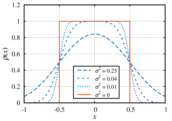
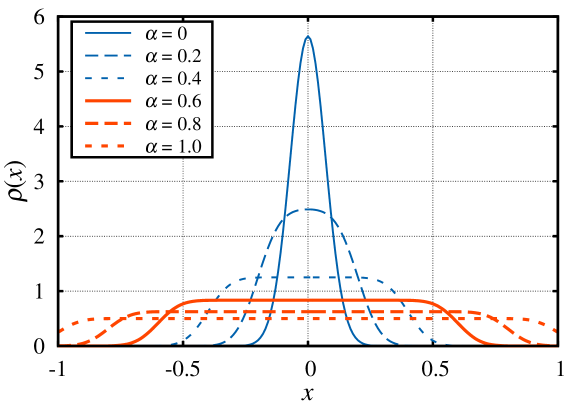
Figure 1: Steady-state distribution of beliefs under unbounded confidence and in the case of homogeneous agents and constant mutual influence. (Top) Impact of the endogenous noise when $\alpha=0.5$. (Bottom) Impact of users’ stubbornness ($\alpha$) when endogenous noise is constant ($\sigma^{2}=0.01$).

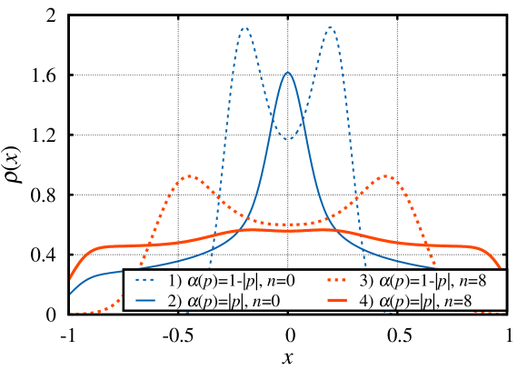
Figure 2: Steady-state distribution of beliefs under unbounded confidence and in the case of inhomogeneous agents and asymmetric mutual influence, different levels of stubbornness, and $\sigma^{2}=0.01$.

Homogeneous agents and constant mutual influence. In this case we consider that all agents exhibit the same level of stubbornness ($\alpha(p)=\alpha$) and the strength of their interaction does not depend on their beliefs or personality ($\zeta_{1}(p)=\zeta_{2}(p^{\prime})=1$). Also, we assume a uniform distribution of agents’ personality over $\mathcal{P}=[-1,1]$, i.e., $\rho_{0}(p)=1/2$, $p\in\mathcal{P}$.

In this case, from (13), we get $\eta(p)=1$ and $w(p)=1$, and, from (24) we obtain the following simple closed-form expression for the steady-state distribution:

$$\rho(x)=\frac{1}{4\alpha}\left[{\rm erf}\left(\frac{\alpha+x}{\sigma}\right)+{\rm erf}\left(\frac{\alpha-x}{\sigma}\right)\right].$$

The results are presented in the plots in Fig. 1, which show the significant role played on $\rho(x)$ by, respectively, the noise variance $\sigma^{2}$ and the parameter $\alpha$.

We observe that when the impact of the endogenous noise is negligible ($\sigma^{2}\to 0$), the belief steady-state distribution becomes uniform as the personality distribution, although more concentrated around 0. As $\sigma^{2}$ increases, the noise process tends to dominate over the agents’ interactions, and the belief distribution tends to become smoother (see Fig. 1(top)). We remark that, since our expressions cannot be directly applied when $\sigma^{2}=0$, this case has been extrapolated as limiting trajectory for the steady-state distribution when $\sigma^{2}\to 0$.

Then in Fig. 1(bottom) we set $\sigma^{2}=0.01$ and let the level of stubbornness, $\alpha$, vary. We note that in the case of highly fickle agents (i.e., $\alpha\to 0$), the belief distribution tends to concentrate around 0, and consensus is not reached only because of the noise (note that also the curve for $\alpha=0$ is obtained as a limit). Indeed, by letting both $\alpha$ and $\sigma^{2}$ tend to 0, it can be easily shown that the steady-state distribution tends to a Dirac measure centered in 0. As $\alpha$ increases, agents become less and less sensitive to others’ beliefs, weighting more their own prejudice. As a result, beliefs are increasingly spread out as $\alpha$ grows. For $\alpha=1$, all agents are stubborn (i.e., completely insensitive to others’ beliefs), thus the steady-state distribution closely resembles the one of the prejudice, and the differences are only due to the presence of noise.

Inhomogeneous agents and asymmetric mutual influence. We now consider a more complex scenario where both agents’ stubbornness and their mutual influence depend on the agents’ personality. In particular, we recall that $u(p)=p$ and we set $\zeta_{1}(p)=1$ and $\zeta_{2}(p^{\prime})=(\alpha(p^{\prime}))^{n}$, i.e., the more stubborn an agent is, the higher her influence on others’ beliefs.

Fig. 2 depicts $\rho(x)$ in the following scenarios:

1. $\alpha(p)=1-|u(p)|=1-|p|$ and $n=0$;

2. $\alpha(p)=|u(p)|=|p|$ and $n=0$;

3. $\alpha(p)=1-|u(p)|=1-|p|$ and $n=8$;

4. $\alpha(p)=|u(p)|=|p|$ and $n=8$.

In scenarios 1) and 3), stubborn agents have a “neutral value” as prejudice (i.e., prejudice equal to 0), while in scenarios 2) and 4) stubborn agents have extremal prejudices (i.e., equal to 1 or $-1$). Moreover, in scenarios 1) and 2) all agents exert the same (high) degree of influence (i.e., $\zeta_{2}(p^{\prime})=1$). Instead, in scenarios 3) and 4), agents exert different degrees of influence, with stubborn agents being the top influential ones and most of the remaining agents exerting marginal influence on other agents.

As expected, in the case in which stubborn users have neutral belief (dotted lines in Fig. 2), they tend to attract other agents, shifting their beliefs toward the center. Such an action is not completely successful since the other agents are still conditioned by their prejudice and the probability mass corresponding to stubborn agents is limited. Comparing scenario 1) to scenario 3) (dotted lines, blue and red, respectively), we can observe that in the former case the mutual influence between fickle agents reinforces the attractive effect of stubborn agents. When instead stubborn agents have extremal beliefs, i.e., in scenarios 2) and 4) denoted by solid lines in Fig. 2, the attractive influence on others exerted by stubborn agents with positive belief, is almost nullified by the attractive influence exerted by stubborn agents with negative belief. Therefore, the vast majority of fickle users tend to converge toward a neutral belief, due to the mutual attraction between themselves. This effect of convergence toward the center tends to vanish as the mutual attraction between fickle agents becomes weaker (i.e., $n$ increases).

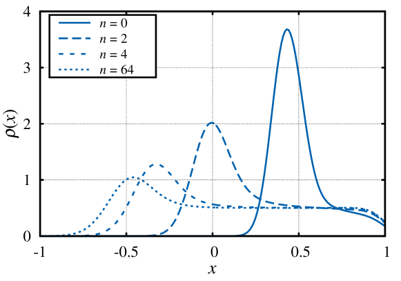
Figure 3: Belief steady-state distribution under unbounded confidence and in the case of proximity-based influence. Stubborn users have biased positive prejudice, and $\sigma^{2}=0.01$.

4.2 Unbounded confidence with $\zeta(|x,x^{\prime}|,p,p^{\prime})=\zeta(p,p^{\prime})$

Now we move to the more general case in which $\zeta$ cannot be expressed in product form. In this case, our goal is to assess the possible effects of the underlying social structure (social graph) on the belief dynamics. We still consider a scenario in which agents’ personalities are uniformly distributed over $\mathcal{P}=[-1,1]$ and $u(p)=p$.

Proximity-based mutual influence. We set $\alpha(p)=(p+1)^{2}/4$, so that stubborn users are those with $p=1$ while fickle users are those with $p=-1$ (hence, they have biased positive and negative prejudice, respectively). We compare scenarios obtained by selecting $\zeta(p,p^{\prime})=\frac{2}{1+(5|p-p^{\prime}|)^{n}}$ for different values of $n$. This expression for $\zeta(p,p^{\prime})$ allows us to study several interesting cases. For $n=0$, it reduces to the case in which $\zeta$ is constant, namely, $\zeta=1$. As $n$ increases, the attraction between agents with similar prejudice (i.e., whenever $|p-p^{\prime}|<1/5$) tends to become stronger ( $\zeta(p,p^{\prime})$ for $|p-p^{\prime}|<1/5$ saturates to 2 as $n\to\infty$), while the attraction between agents with different prejudice (i.e., $|p-p^{\prime}|>1/5$) tends to vanish. It follows that, although we consider the unbounded case, users only interact with other agents in their “proximity”.

Fig. 3 shows the results for a decreasing interaction strength ($n=0,2,4,64$). As expected, the underlying social structure plays a relevant role in the belief dynamics, as it mitigates the ability of stubborn agents to attract other agents.

Community-based mutual influence. Now, we consider a case of practical relevance where two communities of users, with opposite biased prejudice, may interact. We express the level of interaction between the two communities by the parameter $\kappa$, and set the mutual influence to $\zeta(p,p^{\prime})=\frac{1}{2}+\frac{1}{2}\mbox{\rm erf}(pp^{\prime}/\kappa)$. Note that, the larger the $\kappa$, the stronger the mutual influence. Fig. 4(top) depicts the belief distribution when the two communities exhibit a perfectly symmetric structure in terms of agents’ stubbornness and strength of interactions within each community. The plot highlights the importance of interaction between users belonging to two different communities, in view of reaching a global agreement. Indeed, as $\kappa$ (hence the interaction between communities) increases, users’ beliefs tend to mix, and an agreement is essentially reached for $\kappa=10$.

Fig. 4(bottom) instead shows the belief distribution in a similar scenario where stubborn users are now present only in the community characterized by biased positive prejudice. Interestingly, for very small values of $\kappa$ (i.e., when the interaction within each community dominates), the community with negative prejudice (the weak community) reaches a local agreement around its center of mass, while the other (the strong community) remains anchored to the belief of its stubborn agents. As the inter-community interaction increases, the beliefs of the weak community tend to move toward those of the strong one. In particular, for a given level of interaction, the distance between the communities’ beliefs decreases significantly with respect to the case described in the top plot. We also remark that the average belief is now always biased toward the opinion of the strong community, further underlying the importance of the role of stubborn users in belief dynamics.

We remark that similar behaviors have been observed in sociology studies such as [22] and references therein.

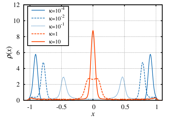
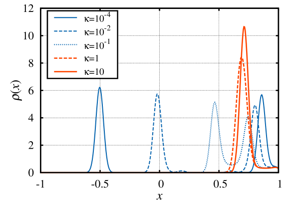
Figure 4: Steady-state belief distribution under unbounded confidence and in the case of community-based influence, as the level of interaction ($\kappa$) varies. Stubborn users are present in both communities (top), or in only one community (bottom).

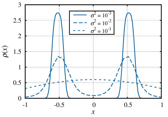
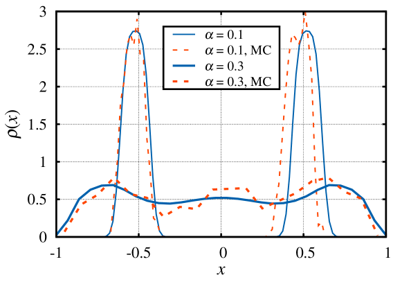
Figure 5: Steady-state belief distribution under bounded confidence, when all agents have the same level of stubbornness and mutual influence vanishes with the distance between agents’ beliefs: (top) impact of the endogenous noise; (bottom) impact of agents’ stubbornness. The bottom plot also presents Monte Carlo (MC) simulation results.

4.3 Bounded confidence

Here we consider the most challenging scenario in which bounded confidence is accounted for. We recall that the results presented in this case can be numerically obtained through the successive approximation technique described in Sec. 3.3.1.

We assume that the agents’ personality is uniformly distributed in $\mathcal{P}=[-1,1]$, agents’ stubbornness is constant ($\alpha(p)=\alpha$), and $u(p)=p$. Also, the mutual influence is a smooth approximation of a centered rectangular function , whose support is given by $|x-x^{\prime}|\leq 1/3$. Fig. 5(top) shows the belief distribution for $\alpha=0.1$ and different variance of the endogenous noise. As previously observed in the literature [11], a clusterization of the agents’ beliefs may occur for effect of the bounded confidence. In particular, for small values of $\sigma^{2}$ (i.e., $\sigma^{2}=10^{-3}$) agents’ beliefs are well partitioned into two distinct clusters centered around $-0.5$ and $0.5$, respectively. The inter-distance of clusters is sufficiently large that agents in the two clusters do not interact, while agents within the same cluster are mutually attracted. By increasing $\sigma^{2}$, the spread of beliefs within each cluster grows, and the clusters start to “interfere” ($\sigma^{2}=10^{-2}$) as a consequence of the reduced distance between the cluster tails. Then clusters completely disappear as the noise variance further increases ($\sigma^{2}=0.1$).

Next, in Fig. 5(bottom) we look at the impact of agents’ stubbornness. This parameter too plays a significant role: increasing $\alpha$ to 0.3 makes clusterization vanish, even for small values of $\sigma^{2}$. The reason is that the higher the $\alpha$, the weaker the mutual attraction between agents’ belief and, the smaller the deviation from the original prejudice. For the sake of validation of our semi-analytical technique, Fig. 5(bottom) reports also the long-run distribution of the agents’ belief obtained with a Monte Carlo simulator, in the case where the system includes $1000$ agents and beliefs evolve according to (1).

5 Transient analysis under unbounded confidence

This section addresses the time evolution of agent’s beliefs under the hypothesis of unbounded confidence (i.e., $\zeta(|x^{\prime}-x|,p,p^{\prime})=\zeta(p,p^{\prime})$) and $\mathcal{X}=\mathbb{R}$.

In this case, the expression of $\mu_{x}(p,x,t,\rho)$ in (5) becomes

$$\mu_{x}(p,x,t,\rho)=\bar{\alpha}(p)\eta(p)\left[\phi(p,t)-x\right]+\alpha(p)[u(p)-x]$$

where $\eta(p)$ is defined in (13) and

$$\phi(p,t)\triangleq\frac{1}{\eta(p)}\int_{\mathcal{Z}}x^{\prime}\zeta(p,p^{\prime})\rho(p^{\prime},x^{\prime},t){\rm\,d}x^{\prime}{\rm\,d}p^{\prime},$$ (25)

is the extension of $\phi(p)$ (defined as the ratio of (14) and (13)) to the transient analysis.

In this case, the FP equation describes an Ornstein-Uhlenbeck random process, whose Green function (impulse response) can be obtained by the method of characteristics, as shown in Appendix E. So doing, we obtain that, for a given value of $p$ and starting from a mass point in $x=u(p)$, the agent density in the belief dimension is Gaussian with mean

$$m(p,t) = {\rm e}^{-w(p)t}u(p)+[1-{\rm e}^{-w(p)t}]\frac{\alpha(p)u(p)}{w(p)}$$ (26)

$$\quad+\bar{\alpha}(p)\eta(p)\int_{0}^{t}{\rm e}^{w(p)(\tau-t)}\phi(p,\tau){\rm\,d}\tau$$

and variance $\sigma^{2}(p,t)=\sigma^{2}(1-{\rm e}^{-2w(p)t})/(2w(p))$ where, we recall that $w(p)=\alpha(p)+\bar{\alpha}(p)\eta(p)$. We remark that $m(p,t)$ in (26) is composed of three terms. The first, which eventually fades away with time constant $1/w(p)$, is due to the initial condition. The second term, which includes a stationary contribution, contains the prejudice of the agents with personality $p$. The third term is related to the interaction between agents. Also, $\lim_{t\to\infty}m(p,t)=m(p)$, as defined in (16).

However, notice that $m(p,t)$ above is a function of $\phi(p,t)$, which is in turn a function of $\rho(p,x,t)$ (see (25)). As such, we have to impose a self-consistency condition, as we have done for the stationary analysis. Precisely, the solution must satisfy

$$\phi(p,t) = \frac{1}{\eta(p)}\int_{\mathcal{P}}\zeta(p,p^{\prime})\int_{\mathbb{R}}x\rho(p^{\prime},x,t){\rm\,d}x{\rm\,d}p^{\prime}$$ (27)

$$= \frac{1}{\eta(p)}\int_{\mathcal{P}}\zeta(p,p^{\prime})\rho_{0}(p^{\prime})\int_{\mathbb{R}}x\frac{{\rm e}^{-\frac{(x-m(p^{\prime},t))^{2}}{2\sigma^{2}(p^{\prime},t)}}}{\sqrt{2\pi\sigma^{2}(p^{\prime},t)}}{\rm\,d}x{\rm\,d}p^{\prime}$$

$$= \frac{1}{\eta(p)}\int_{\mathcal{P}}\zeta(p,p^{\prime})\rho_{0}(p^{\prime})m(p^{\prime},t){\rm\,d}p^{\prime}$$

$$= I_{0}(p,t)+I_{1}(p,t)+\frac{1}{\eta(p)}\int_{\mathcal{P}}\zeta(p,p^{\prime})\rho_{0}(p^{\prime})\bar{\alpha}(p^{\prime})$$

$$\quad\cdot\eta(p^{\prime})\int_{0}^{t}{\rm e}^{w(p^{\prime})(\tau-t)}\phi(p^{\prime},\tau){\rm\,d}\tau{\rm\,d}p^{\prime}$$

where we have defined for brevity:

$$I_{0}(p,t)\triangleq\frac{1}{\eta(p)}\int_{\mathcal{P}}\zeta(p,p^{\prime})\rho_{0}(p^{\prime}){\rm e}^{-w(p^{\prime})t}u(p^{\prime}){\rm\,d}p^{\prime}$$

$$I_{1}(p,t)\triangleq\!\frac{1}{\eta(p)}\int_{\mathcal{P}}\zeta(p,p^{\prime})\rho_{0}(p^{\prime})(1-{\rm e}^{-w(p^{\prime})t})\frac{\alpha(p^{\prime})u(p^{\prime})}{w(p^{\prime})}{\rm\,d}p^{\prime}\,.$$

In order to solve (27) for $\phi(p,t)$, we take its Laplace transform over time (whose variable will be denoted by $s$) and get

$$\widehat{\phi}(p,s) = \widehat{I}_{0}(p,s)\mathord{+}\widehat{I}_{1}(p,s)\mathord{+}\frac{1}{\eta(p)}\int_{\mathcal{P}}\zeta(p,p^{\prime})\rho_{0}(p^{\prime})\bar{\alpha}(p^{\prime})$$ (28)

$$\quad\cdot\eta(p^{\prime})\frac{\widehat{\phi}(p^{\prime},s)}{s+w(p^{\prime})}{\rm\,d}p^{\prime}$$

where $\widehat{\phi}(p,s)$, $\widehat{I}_{0}(p,s)$ and $\widehat{I}_{1}(p,s)$ are the Laplace transforms of $\phi(p,t)$, $I_{0}(p,t)$ and $I_{1}(p,t)$, respectively. Eq. (28) is the integral equation for the transient analysis, which corresponds to (17) in the stationary solution.

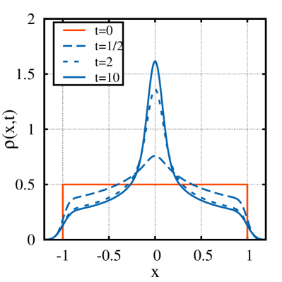
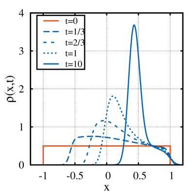
Figure 6: Time evolution of the belief distribution for $\sigma^{2}=0.01$ and constant mutual influence. (Left) Stubborn users have biased prejudice ($\alpha(p)=|p|$); (Right) stubborn users have prejudice biased toward 1.

In the particular case where $\zeta(p,p^{\prime})\equiv\zeta_{1}(p)\zeta_{2}(p^{\prime})$, we have that $\widehat{\phi}(p,s)$, $\widehat{I}_{0}(p,s)$ and $\widehat{I}_{1}(p,s)$ in (28) do not depend anymore on $p$, and, as a consequence, (28) reduces to

$$\widehat{\phi}(s)=\frac{\widehat{I}_{0}(s)+\widehat{I}_{1}(s)}{1-\widehat{I}_{2}(s)}$$ (29)

where $\widehat{I}_{2}(s)=\int_{\mathcal{P}}\zeta_{1}(p)\zeta_{2}(p)\frac{\rho_{0}(p)\bar{\alpha}(p)}{s+w(p)}{\rm\,d}p$. In conclusion, we obtain an explicit solution for $\widehat{\phi}(s)$ (in the Laplace domain), whose singularities are the values of $s$ for which $\widehat{I}_{2}(s)=1$.

Notice that, if $\alpha(p)$ takes only a finite number of values, so does $w(p)$ and the resulting $\widehat{\phi}(s)$ is a rational function, which can be inverse-transformed. In particular, suppose $\alpha(p)\equiv\alpha$. Then $w(p)\equiv w$ and all the integrals can be explicitly computed. If $\overline{m}(t)$ is the average belief at time $t$, i.e.,

$$\overline{m}(t)\triangleq\int_{\mathcal{P}}m(p,t){\rm\,d}p\,,$$

it can be easily found that $\overline{m}(t)=\overline{u}$ where $\overline{u}$ is the average prejudice value.

6 Results on the transient belief distribution

The time evolution of the belief distribution, $\rho(x,t)=\int_{\mathcal{P}}\rho(p,x,t){\rm\,d}p$, is depicted in Figs. 6 and 7 for $u(p)=p$.

Constant mutual influence. Here we show the results obtained for constant mutual influence (i.e., $\zeta=1$). Fig. 6(left) refers to the case of stubborn agents with extremal prejudices ($\alpha(p)=|p|$). Fig. 6(right), instead, corresponds to the case where stubborn users are those with $p=1$ ($\alpha(p)=(p+1)^{2}/4$). We remark that in both cases $\rho(p,x,t)$ can be computed through the analytical expressions presented in the previous subsection. Specifically, we have $\phi(p,t)=0$ for the case outlined in Fig. 6(left), and $\phi(p,t)=\frac{1}{2}\mathbbm{1}_{\{t>0\}}$ for the case shown in Fig. 6(right). In both cases, the dominant time constant is $1/w(p)=1$, and we have observed that $\rho(x,10)$ already closely matches the steady-state distributions.

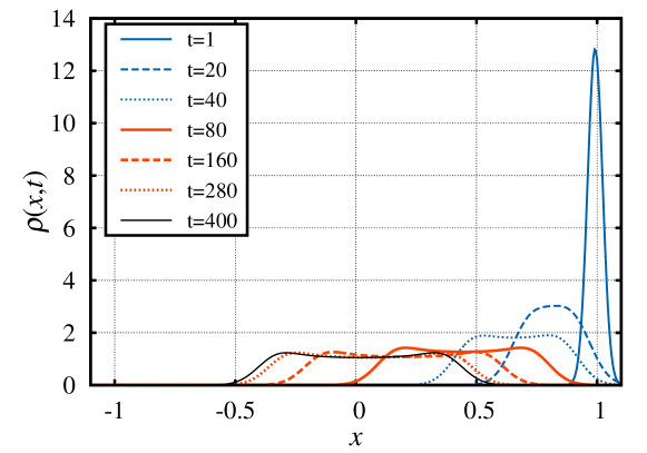
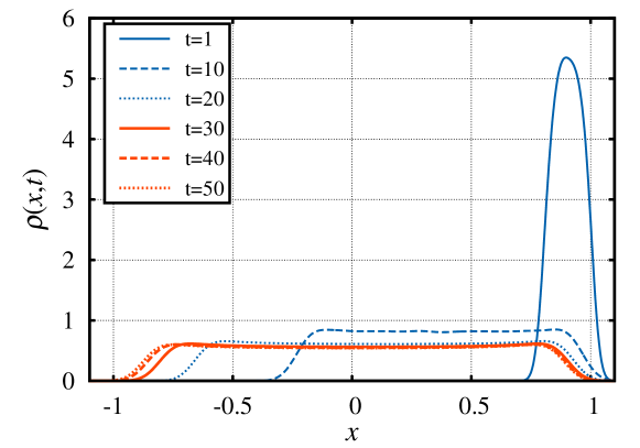
Figure 7: Time evolution of the belief distribution when the mutual influence increases with prejudice similarity and the initial belief density is Gaussian with mean equal to 1. The value of agents’ stubbornness is constant: (top) low stubbornness ($\alpha=0.01$); (bottom) high stubbornness ($\alpha=0.1$).

Event-driven time evolution. Fig. 7 shows the evolution of the belief distribution over time, right after an event that has strongly affected the agents’ belief. We stress that such scenario has been addressed in sociology studies, and similar phenomena have been observed (see, e.g., [21]). A typical example is the impact of breaking news on the public opinion. We model such a situation with a Gaussian distribution with mean equal to 1 and very small variance ($10^{-4}$).

We consider a case where agents show the same level of stubbornness, and the closer the agents’ prejudice, the stronger the interaction ($\zeta(p,p^{\prime})=(1+(p-p^{\prime})^{2})^{-1}$). The top plot refers to the scenario with fickle agents ($\alpha=0.01$); in this case the convergence to the steady-state distribution is slow. A much faster dynamic is instead observed in the bottom plot, which refers to a higher level of user stubbornness ($\alpha=0.1$). In this case, after the initial event, it takes just 1/10 of the time to return to the steady-state distribution, suggesting that the time constant is inversely proportional to the level of user stubbornness.

7 Related work

Several models appeared in the literature represent social interactions between agents through static graphs. In this representation, often users directly interact only with their neighbors, varying their beliefs for effect of pairwise “attractive” interactions [9, 12]. In particular, agent $i$, interacting with agent $j$, updates her belief, represented by a real number, to a new value, which is a convex combination of her own original belief and the belief of agent $j$. As an alternative, a growing thread of works considers highly dynamical settings, in which every agent may interact, still through pairwise “attractive” interactions, with every other agent in the system [8, 10]. Such models have been applied to describe interactions through on-line forums like Reddit, Popurls or Newsvine, as well as direct face-to-face interactions in crowded places such as meetings and conferences. A third thread of work has modeled social interactions through a graph whose structure varies dynamically [3]. These pieces of work capture the fact that in many social networks, e.g., Twitter, agents dynamically follow or divert from other agents’ beliefs based on interests/beliefs similarity.

Another relevant class of models is represented by the so-called bounded confidence, in which social interactions occur only between agents with similar beliefs [13, 14, 15, 11, 16, 17, 18, 19, 20]. In particular, [19, 20] show how bounded confidence models can be used to represent social interactions between Bayesian decision makers. Relevantly to our work, [15] models the social influence on the global opinion evolution in the case of homogeneous agent interactions. By adopting a mean-field approach, the authors derive a differential equation whose solution asymptotically (when the number of agents grows large) represents the opinion evolution. Mean-field theory is applied to the study of opinion dynamics also in [11], where Garnier et al. derive a FP equation modeling the time evolution of beliefs in a neighborhood of $t=0$, in the case of a large number of agents. Through their model, the authors obtain conditions under which a clusterization of the agents’ beliefs occurs. Another study that is particularly relevant to our work is [4], where Baccelli et al. propose a fairly general model that combines several features of previous representations: (i) agent interactions constrained by a graph, (ii) bounded confidence, and (iii) agent endogenous belief random dynamics. For such a model, the authors derive sufficient and necessary conditions for stability, i.e., conditions under which the relative spread of beliefs keeps finite.

We remark that our work significantly differs from the existing studies. In particular, with respect to [15], our model, hence our analysis, is much more general, since it captures non-homogeneous social interactions, the agents’ prejudice and personality, as well as exogenous random perturbations in the agents’ beliefs. The effect of the agents’ prejudice has been neglected also in [11, 4]. Furthermore, unlike [11], which focuses on early stages of the belief temporal evolution, we aim to study the whole-time evolution of the system in the simple case with no bounded confidence, and the steady-state ($t\to\infty$) under more general conditions. Finally, we stress that the goal of our work is not limited to obtaining results on the system stability (as in [4]), but it also studies the transient and steady-state opinion dynamics.

8 Conclusions

Motivated by the great advent of social networks, we investigated the evolution of beliefs within a social system and how they are affected by the interactions between users. Our model captures all the main features characterizing a social system. Through such model and a mean-field approach, we analyzed the system behavior as the number of users grows large. In particular, by representing the belief evolution through a Fokker-Plank partial differential equation, we studied the steady state as well as the transient behavior of the social system. Our main results include: (i) closed-form expressions for the steady-state distribution, which hold in some relevant cases, and (ii) semi-analytical techniques to obtain the steady-state distribution of social beliefs in the most general cases as well as the transient distribution for a remarkably large class of systems. Our analytical derivations are complemented with numerical results, which show interesting dynamics due to social relationships and different degrees of dependence on the users’ prejudice.

Future work will address the model validation through experiments with real-world, Twitter data sets. To this end, by using existing APIs, we intend to collect tweets related to a 2-3 weeks’ time period around an event of particular interest, such as a political election. This set, organized in chronological order, should be filtered by using hashtags that well represent the selected event; then, a sentiment analysis tool should be run on the filtered set. As done in our work, we can assume that the personality coincides with the prejudice, and we can take the first value of sentiment expressed by a user as her prejudice. Contextually, we will need to track the follower-followee relationship between users appearing in our trace and showing to be sufficiently active. A fair (conservative) approximation would be to consider as follower a user that either re-tweets another user’s message or write a new message referring to it. Finally, we will use part of the obtained data as training set to estimate the model parameters, and the rest as testing to validate the prediction capabilities of our model.

Appendix A Ergodicity of the dynamic system described by (1)

We consider Equation (1) in the main manuscript, with a finite number of agents ($U$) and we show that the agents’ belief exhibits a negative drift outside a compact domain, therefore the associated Markov chain is ergodic.

First, it can be easily seen that ours is not an explosive Markovian model (see [28, Sec. 20.3.1]). Second, we remark that a time-sampled version of our model can be seen as a special case of the Non-Linear State Space (NSS(F)) model defined in [28]. Thus, in light of the fact that the noise term in (1) is Gaussian and additive, the Markov chain describing the dynamics of agents’s belief results to be:

i) $\psi$-irreducible over $\mathcal{Z}=\mathcal{X}\times\mathcal{P}$, where measure $\psi$ is equal to the product measure generated by the Lebesque measure over $\mathcal{X}=\mathbb{R}$ and a discrete measure on $\mathcal{P}$ (see again [28, Sec. 20.3.1 and Th. 6.0.1]);

ii) forward accessible and, hence, a $T$-chain (see [28, Prop. 7.1.5]).

Now observe that we can rewrite (1) as:

$$X_{i}(t+{\rm\,d}t)=X_{i}(t)+\Delta X_{i}(t)dt+\sigma dW_{i}$$

where the belief drift $\Delta X_{i}(t)=\frac{[1-\alpha(P_{i})]}{U}\sum_{j\in\mathcal{U},j\neq i}\zeta(|X_{i}(t)-X_{j}(t)|,P_{i},P_{j})(X_{j}(t)-X_{i}(t))+\alpha(P_{i})(u(P_{i})-X_{i}(t))$.

Next, for ease of presentation, we limit ourselves to consider the set of agents with positive belief $X_{i}(t)$, the same derivation applies to negative values of $X_{i}(t)$ (just changing the sign of both belief and drift). If we consider an agent $k$ s.t. $k\in\operatorname*{arg\,max}_{i}X_{i}(t)$, then:

$$\Delta X_{k}(t)= = \frac{[1-\alpha(P_{k})]}{U}\sum_{j\in\mathcal{U},j\neq k}\zeta(|X_{k}(t)-X_{j}(t)|,P_{k},P_{j})(X_{j}(t)-X_{k}(t))+\alpha(P_{k})(u(P_{k})-X_{k}(t))$$

$$\leq [\alpha(P_{k})u(P_{k})-\alpha(P_{k})X_{k}(t)]$$

$$\leq [\sup_{k}\alpha(P_{k})u(P_{k})-\inf_{k}\alpha(P_{k})X_{k}(t)]$$

where we bounded the first term on the RHS with zero since, by construction, $X_{j}(t)-X_{k}(t)=X_{j}(t)-\max_{i}X_{i}(t)\leq 0$.

Similarly, if we consider an agent $l$, we have:

$$\Delta X_{l}(t) = \frac{[1-\alpha(P_{l})]}{U}\sum_{j\in\mathcal{U},j\neq l}\zeta(|X_{l}(t)-X_{j}(t)|,P_{l},P_{j})(X_{j}(t)-X_{l}(t))+\alpha(P_{l})(u(P_{l})-X_{l}(t))$$

$$= \frac{[1-\alpha(P_{l})]}{U}\sum_{j\in\mathcal{U},j\neq l}\zeta(|X_{l}(t)-X_{j}(t)|,P_{l},P_{j})[(X_{j}(t)-X_{k}(t))+(X_{k}(t)-X_{l}(t))]$$

$$+ \alpha(P_{l})(u(P_{l})-X_{l}(t))$$

$$\leq [\sup_{i}\alpha(P_{i})u(P_{i})-\alpha(P_{l})X_{l}(t))+(1-\alpha(P_{l}))S_{\zeta}(X_{k}(t)-X_{l}(t))]$$

where $S_{\zeta}=\sup_{x_{i},x_{j},P_{i},P_{j}}\zeta(|x_{i}-x_{j}|,P_{i},P_{j})<\infty$ with $x_{i},x_{j}\in\mathbb{R}$. By considering sufficiently large $X_{l}(t)$ such that $X_{l}(t)=(1-\beta_{l})X_{k}(t)$ (with $\beta_{l}<1$), we obtain:

$$\Delta X_{l}(t)\leq[\sup_{i}\alpha(P_{i})u(P_{i})-\alpha(P_{l})(1-\beta_{l})X_{k}(t)+(1-\alpha(P_{l}))S_{\zeta}\beta_{l}X_{k}(t)]\leq\sup_{i}\alpha(P_{i})u(P_{i})-\epsilon X_{k}(t)$$

for any arbitrarily chosen $0<\epsilon<\inf_{i}\alpha(P_{i})$ whenever $\beta_{l}\leq\frac{\alpha(P_{l})-\epsilon}{\alpha(P_{l})+S_{\zeta}(1-\alpha(P_{l}))}$. Thus, given $\beta_{0}=\inf_{i}\frac{\alpha(P_{i})-\epsilon}{\alpha(P_{i})+S_{\zeta}(1-\alpha(P_{i}))}>0$, we have that $\Delta X_{l}(t)\leq\sup_{i}\alpha(P_{i})u(P_{i})-\epsilon X_{k}(t)$, uniformly over all $l$ such that $X_{l}(t)>(1-\beta_{0})X_{k}(t)$. At last, observe that the following holds uniformly on every $l$ whenever $\sup_{\alpha}(P_{i})u(P_{i})\leq\alpha(P_{k})S_{\zeta}X_{k}(t)$:

$$\Delta X_{l}(t)\leq[\sup_{i}\alpha(P_{i})u(P_{i})+(1-\alpha(P_{l})S_{\zeta}X_{k}(t)]\leq S_{\zeta}X_{k}(t)\,.$$

Next, let us define the following Lyapunov function: $\mathcal{L}(t)=\frac{1}{n+1}\sum_{i}X_{i}(t)^{n+1}$ for a sufficiently large odd $n$ such that $\epsilon/3X_{k}(t)^{n+1}>US_{\zeta}X_{k}(t)\left[(1-\beta_{0})X_{k}(t)\right]^{n}$, hence $\epsilon/3>US_{\zeta}(1-\beta_{0})^{n}$.

Then, we can write:

$$\Delta\mathcal{L}(t) = \mathbb{E}\left[\mathcal{L}(t+{\rm\,d}t)-\mathcal{L}(t)\mid\{X_{i}(t)\}_{i}\right]$$

$$= \mathbb{E}\left[\sum_{i}X_{i}^{n}(t)\cdot(\Delta X_{i}(t){\rm\,d}t+\sigma{\rm\,d}W_{i})\right]+o\left(\mathbb{E}\left[\sum_{i}X_{i}^{n}(t)\cdot(\Delta X_{i}(t){\rm\,d}t+\sigma{\rm\,d}W_{i})\right]\right)\,.$$

Now, let us focus on the first term on the RHS of the previous expression and consider that $X_{k}(t)$ is sufficiently large. We get:

$$\mathbb{E}\left[\sum_{i}X_{i}^{n}(t)\cdot(\Delta X_{i}(t){\rm\,d}t+\sigma{\rm\,d}W_{i})\right]$$

$$= \sum_{i}X_{i}^{n}(t)\cdot\Delta X_{i}(t){\rm\,d}t$$

$$= \sum_{l:X_{l}(t)>(1-\beta_{0})X_{k}(t)}X_{l}^{n}(t)\cdot\Delta X_{l}(t){\rm\,d}t$$

$$+ \sum_{l:X_{l}(t)\leq(1-\beta_{0})X_{k}(t)}X_{l}^{n}(t)\cdot\Delta X_{l}(t){\rm\,d}t$$

$$\leq X_{k}^{n}(t)[\alpha(P_{k})u(P_{k})-\alpha(P_{k})X_{k}(t)]{\rm\,d}t$$

$$+ \sum_{l\neq k:X_{l}(t)>(1-\beta_{0})X_{k}(t)}X_{l}^{n}(t)\cdot[\sup_{i}\alpha(P_{i})u(P_{i})-\epsilon X_{k}(t)]{\rm\,d}t$$

$$+ \sum_{l:X_{l}(t)\leq(1-\beta_{0})X_{k}(t)}X_{l}^{n}(t)\cdot S_{\zeta}X_{k}(t){\rm\,d}t$$

$$\leq X_{k}^{n}(t)[\sup_{i}\alpha(P_{i})u(P_{i})-\inf_{i}\alpha(P_{i})X_{k}(t)]{\rm\,d}t+\frac{\epsilon}{3}X_{k}(t)^{n+1}{\rm\,d}t\,.$$

Note that we obtained the second inequality from the first one by bounding the second sum with zero, which holds true when $X_{k}$ is sufficiently large.

Now observe that the term $o\left(\mathbb{E}\left[\sum_{i}X_{i}^{n}(t)\cdot(\Delta X_{i}(t){\rm\,d}t+\sigma{\rm\,d}tW_{i})\right]\right)$, can be assumed smaller than $\epsilon/3X_{k}(t)^{n+1}{\rm\,d}t$, for $X_{k}(t)$ sufficiently large. Thus, we have:

$$\Delta\mathcal{L}(t) \leq X_{k}^{n}(t)\sup_{i}\alpha(P_{i})u(P_{i}){\rm\,d}t-\inf_{i}\alpha(P_{i})X_{k}^{n+1}(t){\rm\,d}t+\frac{2\epsilon}{3}X_{k}^{n+1}(t){\rm\,d}t$$

$$\leq X_{k}^{n}(t)\sup_{i}\alpha(P_{i})u(P_{i}){\rm\,d}t-\frac{\epsilon}{3}X_{k}^{n+1}(t){\rm\,d}t$$

where we exploited the fact that $\epsilon<\inf_{i}\alpha(P_{i})$. At last, chosing $B$ such that

$$X_{k}(t)^{n}\sup_{i}\alpha(P_{i})u(P_{i}){\rm\,d}t\leq\max\left(B^{n}\sup_{i}\alpha(P_{i})u(P_{i}){\rm\,d}t,\frac{\epsilon}{12}X_{k}(t)^{n+1}{\rm\,d}t\right),$$

we can bound:

$$\Delta\mathcal{L}(t) \leq B^{n}\sup_{i}\alpha(P_{i})u(P_{i}){\rm\,d}t-\frac{\epsilon}{4}X_{k}^{n+1}(t){\rm\,d}t\,.$$

It follows that the drift of $\mathcal{L}(t)$ becomes negative outside a compact set. Now, in light of the fact that our system is a $\psi$-irreducible $T$-chain, every compact set is petite (see [28, Th. 6.2.5]). Consequently, we can invoke the counterpart of [28, Th. 14.2.3] for continuous-time processes, in order to state that our Markov chain is $\max|X_{l}|^{n+1}$-regular, and therefore ergodic.

Appendix B Continuity of the map $\phi(p)\to\rho_{\phi(p)}(p,x)$

Our goal is to show that the mapping $\phi(p)\to\rho_{\phi(p)}(p,x)$ is continuous under $\mathbb{L}_{\infty}$ norm, i.e., that

$$\|\rho_{\phi(p)}(p,x)-\rho_{\phi^{*}(p)}(p,x)\|_{\infty}\to 0$$

whenever $\phi(p)\to\phi^{*}(p)$ uniformly, for any arbitrary $\phi^{*}(p)$.

We recall that $w(p)=\alpha(p)+\bar{\alpha}(p)\eta(p)$. By dropping the dependency on $p$ in the following expressions, we have

$$\|\rho_{\phi}(x)-\rho^{*}_{\phi}(x)\|_{\infty}$$ (30)

$$= \left\|\sqrt{\frac{w}{\pi\sigma^{2}}}\left({\rm e}^{-\frac{w[x-m]^{2}}{\sigma^{2}}}-{\rm e}^{-\frac{w[x-m^{*}]^{2}}{\sigma^{2}}}\right)\rho_{0}\right\|_{\infty}$$

$$\leq K^{\infty}\left\|{\rm e}^{-\frac{w[x-m]^{2}}{\sigma^{2}}}-{\rm e}^{-\frac{w[x-m^{*}]^{2}}{\sigma^{2}}}\right\|_{\infty}$$

where $K^{\infty}=\|\sqrt{\frac{w}{\pi\sigma^{2}}}\rho_{0}\|_{\infty}$, $m$ is defined in [OurPaper, eq. (15)] and $m^{*}$ is given in [OurPaper, eq. (15)] where $\phi$ is replaced with $\phi^{*}$. Observe that, for any continuously differentiable function $f(x)$, we can write $f(x+m-m^{*})=f(x)+\int_{0}^{m-m^{*}}f^{\prime}(x+y){\rm\,d}y=f(x)+(m-m^{*})f^{\prime}(x+\xi)$ with $\xi\in[0,m-m^{*}]$, where in the last equality we used the mean value theorem for integrals. Thus, $|f(x+m-m^{*})-f(x)|\leq|m-m^{*}|\sup|f^{\prime}(x)|$. Then we have

$$\left\|{\rm e}^{-\frac{w(x-m)^{2}}{\sigma^{2}}}\mathord{-}{\rm e}^{-\frac{w(x-m^{*})^{2}}{\sigma^{2}}}\right\|_{\infty} \leq |m\mathord{-}m^{*}|\sup_{x}\left[\frac{{\rm\,d}e^{-\frac{wx^{2}}{\sigma^{2}}}}{{\rm\,d}x}\right]$$ (31)

$$= |m\mathord{-}m^{*}|\sup_{x}\frac{2wx}{\sigma^{2}}{\rm e}^{-\frac{wx^{2}}{\sigma^{2}}}$$

$$< \sqrt{\frac{2w}{\sigma^{2}{\rm e}}}|m-m^{*}|\,.$$

Therefore, combining (30) and (31), we have:

$$\left|{\rm e}^{-\frac{w(x-m)^{2}}{\sigma^{2}}}-{\rm e}^{-\frac{w(x-m)^{2}}{\sigma^{2}}}\right|\leq\sqrt{\frac{2w}{\sigma^{2}{\rm e}}}\frac{\bar{\alpha}\eta}{w}|\phi-\phi^{*}|$$

and finally:

$$\|\rho_{\phi}(x)-\rho_{\phi^{*}}(x)\|_{\infty}\leq K^{\infty}\sqrt{\frac{2w}{\sigma^{2}{\rm e}}}\frac{\bar{\alpha}\eta}{w}|\phi^{*}-\phi|$$

which goes uniformly to $0$ as $\phi\to\phi^{*}$ uniformly, under the assumption that $\sup_{p}\rho_{0}(p)<\infty$.

Appendix C Continuity of the operator $\mathcal{A}$

Theorem 4

The operator $\mathcal{A}$ is continuous at the fixed point with respect to norm $\mathbb{L}_{1}$ convergence, whenever $\mathcal{X}$ compact, or $\mathcal{X}=\mathbb{R}$ and $\zeta(p,p^{\prime},|x-x^{\prime}|)=0$ for $|x-x^{\prime}|>X_{0}<\infty$.

We now prove the continuity of the operator $\mathcal{A}\{\cdot\}$ around the fixed point. To this end, let $\rho^{*}(p,x)$ be the fixed point of the operator $\mathcal{A}\{\cdot\}$, i.e., $\rho^{*}(p,x)=\mathcal{A}\{\rho^{*}(p,x)\}$. Let us consider a perturbation of the fixed point solution

$$\tilde{\rho}(p,x)=\rho^{*}(p,x)+\epsilon\rho(p,x)$$

where, without lack of generality we assume $\|\rho(p,x)\|_{1}=1$. We have to show that

$$\lim_{\epsilon\to 0}\mathcal{A}\{\tilde{\rho}(p,x)\}=\mathcal{A}\{\rho^{*}(p,x)\}=\rho^{*}(p,x)$$

To this purpose we define

$$\mu_{x,1}(p,x,\rho)=\bar{\alpha}(p)\int_{\mathcal{Z}}\zeta(|x^{\prime}-x|)(x^{\prime}-x)\rho(p^{\prime},x^{\prime}){\rm\,d}x^{\prime}{\rm\,d}p^{\prime}\,.$$ (32)

In the following we drop the dependency on $p$ when not necessary. We note that

$$\mu_{x,1}(x,\tilde{\rho})-\mu_{x,1}(x,\rho^{*})=\mu_{x,1}(x,\tilde{\rho}-\rho^{*})$$

since $\mu_{x,1}(x,\rho)$ is linear w.r.t. the parameter $\rho$. Therefore, we can write the following bound:

$$|\mu_{x,1}(x,\tilde{\rho}-\rho^{*})| = |\mu_{x,1}(x,\epsilon\rho(x))|$$ (33)

$$\leq \bar{\alpha}\epsilon S_{\zeta}X_{0}\int_{\mathcal{Z}}\rho(p^{\prime},x^{\prime}){\rm\,d}x^{\prime}{\rm\,d}p^{\prime}$$

$$\leq \epsilon S_{\zeta}X_{0}$$

where we exploited the fact that $\rho(x)$ is a distribution, $S_{\zeta}=\sup_{|x^{\prime}-x|,p,p^{\prime}}\zeta(|x^{\prime}-x|,p,p^{\prime})<\infty$ and we assumed that $\zeta(|x^{\prime}-x|,p,p^{\prime})=0$ for $|x^{\prime}-x|>X_{0}$. Therefore, using [OurPaper, eq. (10)], we can write:

$$\mathcal{A}\{\tilde{\rho}(x)\} = K{\rm e}^{\frac{2\bar{\alpha}}{\sigma^{2}}\int_{0}^{x}\int_{\mathcal{P},x^{\prime}}\zeta(|x^{\prime}-y|)(x^{\prime}-y)\rho^{*}(p^{\prime},x^{\prime}){\rm\,d}p^{\prime}{\rm\,d}x^{\prime}{\rm\,d}y}$$ (34)

$$\cdot{\rm e}^{\frac{2\bar{\alpha}}{\sigma^{2}}\int_{0}^{x}\int_{\mathcal{P},x^{\prime}}\zeta(|x^{\prime}-y|)(x^{\prime}-y)\epsilon\rho(p^{\prime},x^{\prime}){\rm\,d}p^{\prime}{\rm\,d}x^{\prime}{\rm\,d}y}$$

$$\cdot{\rm e}^{-\frac{\alpha[x-u]^{2}}{\sigma^{2}}}\rho_{0}$$

$$= K{\rm e}^{\frac{2}{\sigma^{2}}\int_{0}^{x}\mu_{x,1}(y,\rho^{*}){\rm\,d}y}{\rm e}^{\frac{2}{\sigma^{2}}\int_{0}^{x}\mu_{x,1}(y,\epsilon\rho)]{\rm\,d}y}$$

$$\cdot{\rm e}^{-\frac{\alpha[x-u]^{2}}{\sigma^{2}}}\rho_{0}$$

Now, defined $v(x)=\frac{1}{x}\int_{0}^{x}\mu_{x,1}(y,\epsilon\rho){\rm\,d}y$ (with $v(0)=0$), we have:

$$\mathcal{A}\{\tilde{\rho}(x)\} = K^{\prime}{\rm e}^{\frac{2}{\sigma^{2}}\int_{0}^{x}\mu_{x,1}(y,\rho^{*}){\rm\,d}y}\cdot{\rm e}^{-\frac{\alpha}{\sigma^{2}}[x-u-v(x)]^{2}}\rho_{0}$$

where $K^{\prime}=K{\rm e}^{-[2uv(x)+v(x)^{2}/\alpha]}$. Since $|\int_{0}^{x}\mu(y,\epsilon\rho){\rm\,d}y|\leq\epsilon S_{\zeta}X_{0}x$, and

$$\mathcal{A}\{\rho^{*}(x)\}=\rho^{*}(x)=K{\rm e}^{2\frac{\int_{0}^{x}\mu_{x,1}(y,\rho^{*}){\rm\,d}y}{\sigma^{2}}}{\rm e}^{-\frac{\alpha(x-u)^{2}}{\sigma^{2}}}\rho_{0}$$

subtracting $\mathcal{A}\{\rho^{*}(x)\}$ from both sides of (C), we have:

$$\mathcal{A}\{\tilde{\rho}(x)\}-\mathcal{A}\{\rho^{*}(x)\}$$ (36)

$$= K^{\prime}{\rm e}^{2\frac{\int_{0}^{x}\mu_{x,1}(y,\rho^{*}){\rm\,d}y}{\sigma^{2}}}{\rm e}^{-\frac{\alpha[(x-u-v(x))^{2}}{\sigma^{2}}}\rho_{0}$$

$$-K{\rm e}^{2\frac{\int_{0}^{x}\mu_{x,1}(y,\rho^{*}){\rm\,d}y}{\sigma^{2}}}{\rm e}^{-\frac{\alpha[(x-u)^{2}}{\sigma^{2}}}\rho_{0}$$

$$\leq \rho^{*}(x)\left(\frac{K^{\prime}}{K}{\rm e}^{-\frac{\alpha[x-u-v(x)]^{2}}{\sigma^{2}}+\frac{\alpha[(x-u)^{2}}{\sigma^{2}}}-1\right)\,.$$

Note that

$${\rm e}^{-\frac{\alpha[x-u-v(x)]^{2}}{\sigma^{2}}+\frac{\alpha[(x-u)^{2}}{\sigma^{2}}}={\rm e}^{-\frac{\alpha v(x)^{2}}{\sigma^{2}}+\frac{2\alpha(x-u)v(x)}{\sigma^{2}}}$$

Since $|v(x)|\leq\epsilon S_{\zeta}X_{0}\to 0$ as $\epsilon\to 0$, then the above quantity tends to 1 uniformly. Similarly, $K^{\prime}/K\to 1$ uniformly for any $p$. Thus, the term $|\mathcal{A}\{\tilde{\rho}(x)\}-\mathcal{A}\{\rho^{*}(x)\}|\to 0$ as $\epsilon\to 0$.

When $\mathcal{X}$ is a finite interval, continuity of the operator $\mathcal{A}\{\cdot\}$ can be proven under general conditions on $\zeta(p,p^{\prime},|x-x^{\prime}|)$ by uniformly bounding $|\mu_{x,1}(x,\tilde{\rho}-\rho^{*})|$ and then applying the same arguments as before.

Appendix D On the local/global contraction properties of operator $\mathcal{A}\{\cdot\}$ under compact $\mathcal{X}$

Without loss of generality, let us consider the set $\mathcal{X}$ as symmetric with respect to 0 and define

$$\|\rho(p,x)\|_{1}=\int_{\mathcal{Z}}|\rho(p,x)|{\rm\,d}x{\rm\,d}p$$

Observe that the class of probability density functions (i.e., functions $\rho(p,x)\geq 0$ with $\|\rho(p,x)\|_{1}=1$) forms an invariant set under the operator $\mathcal{A}\{\cdot\}$ (i.e., any probability density function $\rho(p,x)$ is mapped by $\mathcal{A}$ onto a probability density function). Furthermore, note that if $\rho^{(k)}(p,x)$ is a probability density, then $\rho^{(k+1)}(p,x)=\mathcal{A}\{\rho^{(k)}(p,x)\}$ belongs to the same class. It follows that we can limit our analysis to the case where the operator $\mathcal{A}\{\cdot\}$ is applied on probability densities.

In order to show that the operator $\mathcal{A}\{\cdot\}$ is a contraction, we need to show that for any two probability densities, $\rho_{1}(p,x)$ and $\rho_{2}(p,x)$, we have [27]:

$$\|\mathcal{A}\{\rho_{2}(p,x)\}-\mathcal{A}\{\rho_{1}(p,x)\}\|_{1}<c\|\rho_{2}(p,x)-\rho_{1}(p,x)\|_{1}$$ (37)

where $c<1$ and where $\|\cdot\|_{1}$ is the above defined norm. We first apply the operator $\mathcal{A}\{\cdot\}$ on $\rho_{1}(p,x)$ and $\rho_{2}(p,x)$ separately. By the definition of $\mathcal{A}\{\cdot\}$, we have

$$\mathcal{A}\{\rho_{1}(p,x)\}=K_{1}(p){\rm e}^{\frac{2}{\sigma^{2}}\int_{0}^{x}\mu_{x,1}(p,y,\rho_{1}){\rm\,d}y}{\rm e}^{-\frac{\alpha(p)[x-u(p)]^{2}}{\sigma^{2}}}\rho_{0}(p)$$

where the positive normalization factor $K_{1}(p)$ is such that

$$K_{1}(p)^{-1}=\int_{\mathcal{X}}{\rm e}^{\frac{2}{\sigma^{2}}\int_{0}^{x}\mu_{x,1}(p,y,\rho_{1}){\rm\,d}y}{\rm e}^{-\frac{\alpha(p)[x-u(p)]^{2}}{\sigma^{2}}}{\rm\,d}x\,.$$

To proceed further, we observe that $\mu_{x}(p,y,\rho)$ is linear in $\rho$. Indeed [OurPaper, eq. (4)], we have $\mu_{x,1}(p,y,\rho_{1}+\rho_{2})=\mu_{x,1}(p,y,\rho_{1})+\mu_{x,1}(p,y,\rho_{2})$. Let us define $M_{x,1}(p,\rho)=\frac{2}{\sigma^{2}}\int_{0}^{x}\mu_{x,1}(p,y,\rho){\rm\,d}y$ and $G(x,p)={\rm e}^{-\frac{\alpha(p)[x-u(p)]^{2}}{\sigma^{2}}}\rho_{0}(p)$. It follows

$$\mathcal{A}\{\rho_{2}(p,x)\} = K_{2}(p){\rm e}^{M_{x,1}(p,\rho_{2})}{\rm e}^{-\frac{\alpha(p)[x-u(p)]^{2}}{\sigma^{2}}}\rho_{0}(p)$$ (38)

$$= K_{2}(p){\rm e}^{M_{x,1}(p,\rho_{1}+(\rho_{2}-\rho_{1}))}G(x,p)$$

$$= K_{2}(p){\rm e}^{M_{x,1}(p,\rho_{1})+M_{x,1}(p,\rho_{2}-\rho_{1})}G(x,p)$$

$$= K_{2}(p){\rm e}^{M_{x,1}(p,\rho_{1})}{\rm e}^{M_{x,1}(p,\rho_{2}-\rho_{1})}G(x,p)$$

$$= \mathcal{A}\{\rho_{1}(p,x)\}\frac{K_{2}(p)}{K_{1}(p)}{\rm e}^{M_{x,1}(p,\rho_{2}-\rho_{1})}$$

with

$$K_{2}(p)^{-1}=\int_{\mathcal{X}}{\rm e}^{M_{x,1}(p,\rho_{1})}{\rm e}^{M_{x,1}(p,\rho_{2}-\rho_{1})}{\rm e}^{-\frac{\alpha(p)[x-u(p)]^{2}}{\sigma^{2}}}{\rm\,d}x\,.$$ (39)

Therefore,

$$\|\mathcal{A}\{\rho_{2}(p,x)\}-\mathcal{A}\{\rho_{1}(p,x)\}\|_{1}$$ (40)

$$\leq \left\|\mathcal{A}\{\rho_{1}(p,x)\}\left(\frac{K_{2}(p)}{K_{1}(p)}{\rm e}^{M_{x,1}(p,\rho_{2}-\rho_{1})}-1\right)\right\|_{1}$$

$$\leq \left\|\mathcal{A}\{\rho_{1}(p,x)\}\left|\frac{K_{2}(p)}{K_{1}(p)}{\rm e}^{M_{x,1}(p,\rho_{2}-\rho_{1})}-1\right|\right\|_{1}$$

$$\leq \|\mathcal{A}\{\rho_{1}(p,x)\}\|_{1}\sup_{(p,x)}\left|\frac{K_{2}(p)}{K_{1}(p)}{\rm e}^{M_{x,1}(p,\rho_{2}-\rho_{1})}-1\right|$$

$$= \sup_{(p,x)}\left|\frac{K_{2}(p)}{K_{1}(p)}{\rm e}^{M_{x,1}(p,\rho_{2}-\rho_{1})}-1\right|$$

Now, observe that

$$|M_{x,1}(p,\rho_{2}-\rho_{1})| = \left|\frac{2}{\sigma^{2}}\int_{0}^{x}\mu_{x,1}(p,y,\rho_{2}-\rho_{1}){\rm\,d}y\right|$$

$$\leq \frac{2}{\sigma^{2}}\left|\int_{0}^{x}|\mu_{x,1}(p,y,\rho_{2}-\rho_{1})|{\rm\,d}y\right|$$

and

$$|\mu_{x,1}(p,x,\rho_{2}-\rho_{1})|$$

$$= \left|\bar{\alpha}(p)\int_{\mathcal{Z}}\zeta(|x^{\prime}-x|,p,p^{\prime})(x^{\prime}-x)R(p^{\prime},x^{\prime}){\rm\,d}x^{\prime}{\rm\,d}p^{\prime}\right|$$

$$\leq \bar{\alpha}(p)\int_{\mathcal{Z}}\zeta(|x^{\prime}-x|,p,p^{\prime})|x^{\prime}-x|\left|R(p^{\prime},x^{\prime})\right|{\rm\,d}x^{\prime}{\rm\,d}p^{\prime}$$

$$\leq S_{\zeta}X_{0}\|R(p,x)\|_{1}$$

where $R(p,x)=\rho_{2}(p,x)-\rho_{1}(p,x)$, we defined

$$S_{\zeta}=\sup_{x,x^{\prime}\in\mathcal{X}}\zeta(|x^{\prime}-x|,p,p^{\prime})<\infty$$

and assumed $\zeta(p,p^{\prime},|x-x^{\prime}|)=0$ whenever $|x-x^{\prime}|>X_{0}$. Moreover, $\sup\{1-\alpha(p)\}\leq 1$ since $0\leq\alpha(p)\leq 1$. We also observe that by definition $\|\rho(p,x)\|_{1}=1$ for any distribution $\rho(p,x)$. Thus $\forall x\in\mathcal{X}$

$$|M_{x,1}(p,\rho_{2}-\rho_{1})| \leq \frac{2}{\sigma^{2}}\left|\int_{0}^{x}2\bar{\alpha}(p)S_{\zeta}X_{0}\|R(p,x)\|_{1}{\rm\,d}y\right|$$ (42)

$$= \frac{2}{\sigma^{2}}S_{\zeta}X_{0}\|R(p,x)\|_{1}\left|\int_{0}^{x}{\rm\,d}y\right|$$

$$\leq \frac{2}{\sigma^{2}}S_{\zeta}X_{0}|x|\|R(p,x)\|_{1}$$

$$\leq \frac{2}{\sigma^{2}}S_{\zeta}X_{0}S_{x}\|R(p,x)\|_{1}$$

$$= \Delta$$

where $S_{x}=\sup_{x\in\mathcal{X}}|x|<\infty$. The above inequality implies that uniformly on $x$ we have: $-\Delta\leq M_{x,1}(p,\rho_{2}-\rho_{1})\leq\Delta$, i.e.,

$${\rm e}^{-\Delta}\leq{\rm e}^{M_{x,1}(p,\rho_{2}-\rho_{1})}\leq{\rm e}^{\Delta}\,.$$

Furthermore, observe that from (39) we can obtain the following bounds on the normalization factor $K_{2}(p)$:

$$K_{2}(p)^{-1} = \int_{\mathcal{X}}{\rm e}^{M_{x,1}(p,\rho_{1})}{\rm e}^{-\frac{\alpha(p)[x-u(p)]^{2}}{\sigma^{2}}}{\rm e}^{M_{x,1}(p,\rho_{2}-\rho_{1})}{\rm\,d}x$$ (43)

$$\leq K_{1}(p)^{-1}{\rm e}^{\Delta}$$

and

$$K_{2}(p)^{-1} = \int_{\mathcal{X}}{\rm e}^{M_{x,1}(p,\rho_{1})}{\rm e}^{-\frac{\alpha(p)[x-u(p)]^{2}}{\sigma^{2}}}{\rm e}^{M_{x,1}(p,\rho_{2}-\rho_{1})}{\rm\,d}x$$ (44)

$$\geq K_{1}(p)^{-1}{\rm e}^{-\Delta}$$

which can be summarized as

$${\rm e}^{-\Delta}\leq\frac{K_{2}(p)}{K_{1}(p)}\leq{\rm e}^{\Delta}\,.$$

Note also that, for any $|w|<1/2$, we have ${\rm e}^{2|w|}-1\leq 4|w|$ and $1-{\rm e}^{-2|w|}\leq 2|w|$. It follows that for $\Delta<1/2$ the term $|K_{2}(p)/K_{1}(p){\rm e}^{M_{x,1}(p,\rho_{2}-\rho_{1})}-1|$ can be bounded as

$$\left|\frac{K_{2}(p)}{K_{1}(p)}{\rm e}^{M_{x,1}(p,\rho_{2}-\rho_{1})}-1\right| \leq \max\left\{{\rm e}^{2\Delta}-1,1-{\rm e}^{-2\Delta}\right\}$$ (45)

$$\leq \max\left\{4\Delta,2\Delta\right\}$$

$$\leq 4\Delta$$

$$= \frac{8}{\sigma^{2}}S_{\zeta}S_{x}X_{0}\|R(p,x)\|_{1}\,.$$

In conclusion, we get

$$\|\mathcal{A}\{\rho_{2}(p,x)\}-\mathcal{A}\{\rho_{1}(p,x)\}\|_{1}\leq\frac{8}{\sigma^{2}}S_{\zeta}S_{x}X_{0}\|R(p,x)\|_{1}$$ (46)

Therefore, $\mathcal{A}\{\cdot\}$ is a contraction operator if

$$\frac{8S_{\zeta}S_{x}X_{0}}{\sigma^{2}}<1$$

which implies $\frac{S_{\zeta}S_{x}X_{0}}{\sigma^{2}}<\frac{1}{8}$. Note that, by the definition of $\Delta$ given in (42), we have

$$\Delta = \frac{2S_{\zeta}S_{x}X_{0}}{\sigma^{2}}\|R(p,x)\|_{1}$$ (47)

$$\leq 2\frac{1}{8}\|R(p,x)\|_{1}$$

$$\leq \frac{1}{2}$$

since $\|R(p,x)||_{1}\leq\|\rho_{2}(p,x)\|_{1}+\|\rho_{1}(p,x)||_{1}\leq 2$. Thus, the condition $\Delta<\frac{1}{2}$ is met.

Following the same approach, we can easily prove that $\mathcal{A}\{\cdot\}$ is a contraction locally in a neighborhood of $\rho^{*}(p,x)$ (i.e., the fixed point of $\mathcal{A}\{\cdot\}$) whenever $\frac{2S_{\zeta}S_{x}}{\sigma^{2}}<1-\epsilon\quad\forall\epsilon>0$. To this end, it is enough to note that for sufficiently small $w$ and $\forall\epsilon>0$, $e^{w}<1+(1+\epsilon)w$ and that $w/(1-w)<(1+\epsilon)w$.

At last, observe that from (46) we can immediately deduce the continuity at every point of operator $\mathcal{A}\{\cdot\}$ w.r.t. the convergence in norm $\mathbb{L}_{1}$, provided that $S_{\zeta}<\infty$ and $S_{x}<\infty$ (and noticing that by construction $X_{0}\leq 2S_{x}$). Indeed, as $\|\rho_{2}(p,x)-\rho_{1}(p,x)\|_{1}\to 0$, necessarily $\|\mathcal{A}\{\rho_{2}(p,x)\}-\mathcal{A}\{\rho_{1}(p,x)\}\|_{1}\to 0$.

Appendix E Derivation of (57)

Consider the FP equation in [OurPaper, eq. (2)], which, thanks to [OurPaper, eq. (24)], can be written as

$$\begin{split}\frac{\partial}{\partial t}\rho(p,x,t)=&\frac{\partial}{\partial x}[(w(p)x-\psi(p,t))\rho(p,x,t)]+\\ &\,\,\,\,\,\frac{1}{2}\sigma^{2}\frac{\partial^{2}}{\partial x^{2}}\rho(p,x,t)\end{split}$$ (48)

where $w(p)=\alpha(p)+\bar{\alpha}(p)\eta(p)$ and $\psi(p,t)=\bar{\alpha}(p)\eta(p)\phi(p,t)+\alpha(p)u(p)$. In this appendix, we will omit the argument $p$ unless necessary.

In the following, we will derive the Green function (i.e., the impulse response) of this FP equation for an initial condition $\rho(p,x,0)=\delta(x-x^{\prime})\delta(p-p^{\prime})$. To this purpose, let us Fourier-transform from variable $x$ to variable $\nu$, obtaining the first-order PDE

$$\left[\frac{\partial}{\partial t}\mathord{+}w\nu\frac{\partial}{\partial\nu}\right]\widehat{\rho}(p,\nu,t)=\mathord{-}\left[j2\pi\nu\psi(t)\mathord{+}2\pi^{2}\nu^{2}\sigma^{2}\right]\widehat{\rho}(p,\nu,t).$$ (49)

Next, we introduce an auxiliary parameter $u$ and consider $t=t(u)$, $\nu=\nu(u)$ and $\widehat{\rho}=\widehat{\rho}(u)$, with initial conditions $t(0)=0$, $\nu(0)=\nu_{0}$ and

$$\widehat{\rho}(0)=\widehat{\rho}(p,\nu_{0},0)=e^{-j2\pi\nu_{0}x^{\prime}}\delta(p-p^{\prime})$$ (50)

Parameterizing over $u$, we transform the PDE in (49) into a system of ODEs by exploiting the identity

$$\left[\frac{{\rm\,d}t}{{\rm\,d}u}\frac{\partial}{\partial t}+\frac{{\rm\,d}\nu}{{\rm\,d}u}\frac{\partial}{\partial\nu}\right]\widehat{\rho}=\frac{{\rm\,d}\widehat{\rho}}{{\rm\,d}u}\,.$$ (51)

By comparing (49) and (51), we then get

$$\left\{\begin{array}[]{ccl}\frac{{\rm\,d}t}{{\rm\,d}u}&=&1\\ \frac{{\rm\,d}\nu}{{\rm\,d}u}&=&w\nu\\ \frac{{\rm\,d}\widehat{\rho}}{{\rm\,d}u}&=&-\left[j2\pi\nu\psi(u)+2\pi^{2}\nu^{2}\sigma^{2}\right]\widehat{\rho}\end{array}\right.$$ (52)

which is easily solved as

$$t(u)=u,\,\,\,\,\nu(u)=\nu_{0}{\rm e}^{wu}$$ (53)

and

$$\frac{{\rm\,d}\widehat{\rho}}{{\rm\,d}u}=-\left[j2\pi\nu_{0}e^{wu}\psi(u)+2\pi^{2}\sigma^{2}\nu_{0}^{2}e^{2wu}\right]\widehat{\rho}\,.$$ (54)

The solution of (54) is

$$\widehat{\rho}(u) = \widehat{\rho}(0){\rm e}^{-j2\pi\nu_{0}\int_{0}^{u}{\rm e}^{wv}\phi(v){\rm\,d}v}\exp\left(\pi^{2}\sigma^{2}\nu_{0}^{2}\frac{1-{\rm e}^{2wu}}{w}\right)$$ (55)

$$= \delta(p-p^{\prime})\exp\left\{-j2\pi\nu_{0}\left[x^{\prime}+\int_{0}^{u}{\rm e}^{wv}\psi(v){\rm\,d}v\right]\right.$$

$$\left.-\pi^{2}\sigma^{2}\nu_{0}^{2}\frac{{\rm e}^{2wu}-1}{w}\right\}\,.$$

By substituting equations (53) into (55), we finally obtain

$$\widehat{\rho}(p,\nu,t|p^{\prime},x^{\prime}) = \delta(p-p^{\prime})\exp\left\{-j2\pi\nu{\rm e}^{-wt}\left[x^{\prime}\right.\right.$$

$$\left.\left.+\int_{0}^{t}{\rm e}^{w\tau}\psi(\tau){\rm\,d}\tau\right]-\pi^{2}\sigma^{2}\nu^{2}\frac{1-{\rm e}^{-2wt}}{w}\right\}\,.$$

Taking the inverse Fourier transform, we get the Green function of the FP equation as

$$\rho(p,x,t|p^{\prime},x^{\prime}) = \delta(p-p^{\prime})\sqrt{\frac{w}{\pi\sigma^{2}(1-{\rm e}^{-2wt})}}$$

$$\exp\left\{-\frac{w\left(x-{\rm e}^{-wt}\left[x^{\prime}+\int_{0}^{t}{\rm e}^{w\tau}\psi(p,\tau){\rm\,d}\tau\right]\right)^{2}}{\sigma^{2}(1-{\rm e}^{-2wt})}\right\}$$

which, as a function of $x$, is a Gaussian pdf with variance

$$\sigma^{2}(p,t)\triangleq\frac{\sigma^{2}(1-{\rm e}^{-2w(p)t})}{2w(p)}$$ (56)

and mean

$$m(p,x^{\prime},t) \triangleq {\rm e}^{-w(p)t}\left[x^{\prime}+\int_{0}^{t}{\rm e}^{w(p)\tau}\psi(p,\tau){\rm\,d}\tau\right]$$

$$= e^{-w(p)t}x^{\prime}+(1-e^{-w(p)t})\frac{\alpha(p)u(p)}{w(p)}$$

$$+\bar{\alpha}(p)\eta(p)\int_{0}^{t}e^{w(p)(\tau-t)}\phi(p,\tau)d\tau\,.$$

For a general initial density value $\rho(p,x,0)=\rho_{0}(x|p)\rho_{0}(p)$, we obtain the solution of the FP equation $\rho(p,x,t)$ as

$$\rho(p,x,t)=\rho_{0}(p)\int_{\mathcal{Z}}\rho(p,x,t|p^{\prime},x^{\prime})\rho_{0}(x^{\prime}|p^{\prime}){\rm\,d}x^{\prime}{\rm\,d}p^{\prime}.$$ (57)

References

• [1] R. Colbaugh, K. Glass, and P. Ormerod, Predictability and Prediction for an Experimental Cultural Market.   Springer Berlin Heidelberg, 2010, pp. 79–86.
• [2] S. Asur and B. A. Huberman, “Predicting the future with social media,” in IEEE/WIC/ACM International Conference on Web Intelligence and Intelligent Agent Technology, Washington, DC, USA, 2010, pp. 492–499.
• [3] G. Shi, M. Johansson, and K. H. Johansson, “How agreement and disagreement evolve over random dynamic networks,” IEEE Journal on Selected Areas in Communications, vol. 31, no. 6, pp. 1061–1071, 2013.
• [4] F. Baccelli, A. Chatterjee, and S. Vishwanath, “Pairwise stochastic bounded confidence opinion dynamics: Heavy tails and stability,” IEEE Transactions on Automatic Control, 2017.
• [5] M. E. Yildiz, R. Pagliari, A. Ozdaglar, and A. Scaglione, “Voting models in random networks,” in Information Theory and Applications Workshop, 2010, pp. 1–7.
• [6] M. Farajtabar, N. Du, M. Gomez-Rodriguez, I. Valera, L. Song, and H. Zha, “Shaping social activity by incentivizing users,” in NIPS, 2014.
• [7] B. Pang and L. Lee, “Opinion mining and sentiment analysis,” Found. Trends Inf. Retr., vol. 2, no. 1-2, pp. 1–135, Jan. 2008.
• [8] M. H. DeGroot, “Reaching a consensus,” Journal of the American Statistical Association, vol. 69, no. 345, pp. 118–121, 1974.
• [9] N. E. Friedkin and E. C. Johnsen, “Social positions in influence networks,” Social Networks, vol. 19, no. 3, pp. 209–222, 1997.
• [10] D. Acemoglu, G. Como, F. Fagnani, and A. Ozdaglar, “Opinion fluctuations and persistent disagreement in social networks,” in 2011 50th IEEE Conference on Decision and Control and European Control Conference, Dec 2011, pp. 2347–2352.
• [11] J. Garnier, G. Papanicolaou, and T.-W. Yang, “Consensus convergence with stochastic effects,” Vietnam Journal of Mathematics, vol. 1, no. 1, pp. 1–25, March 2016. [Online]. Available: arXiv:1508.07313
• [12] C. Ravazzi, P. Frasca, R. Tempo, and H. Ishii, “Ergodic randomized algorithms and dynamics over networks,” IEEE Transactions on Control of Network Systems, vol. 2, no. 1, pp. 78–87, March 2015.
• [13] G. Deffuant, D. Neau, F. Amblard, and G. Weisbuch, “Mixing beliefs among interacting agents,” Advances in Complex Systems, vol. 03, no. 01n04, pp. 87–98, 2000. [Online]. Available: http://www.worldscientific.com/doi/abs/10.1142/S0219525900000078
• [14] R. Hegselmann and U. Krause, “Opinion dynamics and bounded confidence: models, analysis and simulation,” Journal of Artificial Societies and Social Simulation, vol. 5, no. 3, pp. 87–98, June 2002. [Online]. Available: http://jasss.soc.surrey.ac.uk/5/3/2.html
• [15] G. Como and F. Fagnani, “Scaling limits for continuous opinion dynamics systems,” vol. 21, no. 4.   Institute of Mathematical Statistics, 2011, pp. 1537–1567. [Online]. Available: http://www.jstor.org/stable/23033379
• [16] V. D. Blondel, J. M. Hendrickx, and J. N. Tsitsiklis, “On krause’s multi-agent consensus model with state-dependent connectivity,” IEEE Transactions on Automatic Control, vol. 54, no. 11, pp. 2586–2597, Nov 2009.
• [17] G. Weisbuch, G. Deffuant, F. Amblard, and J.-P. Nadal, “Meet, discuss, and segregate!” Complexity, vol. 7, no. 3, pp. 55–63, 2002. [Online]. Available: http://dx.doi.org/10.1002/cplx.10031
• [18] A. Bhattacharyya, M. Braverman, B. Chazelle, and H. L. Nguyen, “On the convergence of the hegselmann-krause system,” in 4th Conference on Innovations in Theoretical Computer Science, ser. ITCS ’13.   New York, NY, USA: ACM, 2013, pp. 61–66. [Online]. Available: http://doi.acm.org/10.1145/2422436.2422446
• [19] K. R. Varshney, “Bounded confidence opinion dynamics in a social network of bayesian decision makers,” IEEE Journal of Selected Topics in Signal Processing, vol. 8, no. 4, pp. 576–585, Aug 2014.
• [20] L. R. Varshney and K. R. Varshney, “Decision making with quantized priors leads to discrimination,” Proceedings of the IEEE, vol. 105, no. 2, pp. 241–255, Feb 2017.
• [21] H. G. Boomgaarden and C. H. de Vreese, “Dramatic real-world events and public opinion dynamics: Media coverage and its impact on public reactions to an assassination,” International Journal of Public Opinion Research, vol. 19, no. 3, pp. 354–366, 2007.
• [22] A. Baronchelli, “The Emergence of Consensus,” ArXiv e-prints, Apr. 2017.
• [23] J. Gärtner, “On the McKean-Vlasov limit for interacting diffusions,” Mathematische Nachrichten, vol. 137, no. 1, pp. 197–248, 1988.
• [24] D. A. Dawson, “Critical dynamics and fluctuations for a mean-field model of cooperative behavior,” Journal of Statistical Physics, vol. 31, no. 1, pp. 29–85, 1983.
• [25] A. N. Kolmogorov and S. V. Fomin, Elements of the Theory of Functions and Functional Analysis.   Martino Publishing, 2012.
• [26] R. Kress, Linear integral equations.   Springer, 1989.
• [27] A. N. Kolmogorov and S. V. Fomin, Introductory real analysis.   Courier, 2012.
• [28] S. Meyn and R. Tweedie, Markov Chains and Stochastic Stability.   Cambridge University Press, 2009.