A progressive reduced basis/empirical interpolation method for nonlinear parabolic problems

Abstract

We investigate new developments of the combined Reduced-Basis and Empirical Interpolation Methods (RB-EIM) for parametrized nonlinear parabolic problems. In many situations, the cost of the EIM in the offline stage turns out to be prohibitive since a significant number of nonlinear time-dependent problems need to be solved using the high-fidelity (or full-order) model. In the present work, we develop a new methodology, the Progressive RB-EIM (PREIM) method for nonlinear parabolic problems. The purpose is to reduce the offline cost while maintaining the accuracy of the RB approximation in the online stage. The key idea is a progressive enrichment of both the EIM approximation and the RB space, in contrast to the standard approach where the EIM approximation and the RB space are built separately. PREIM uses high-fidelity computations whenever available and RB computations otherwise. Another key feature of each PREIM iteration is to select twice the parameter in a greedy fashion, the second selection being made after computing the high-fidelity solution for the firstly selected value of the parameter. Numerical examples are presented on nonlinear heat transfer problems.

1 Introduction

The Reduced-Basis (RB) method devised in [14, 17] (see also the recent textbooks [11, 18]) is a computationally effective approach to approximate parametrized Partial Differential Equations (PDEs) encountered in many problems in science and engineering. For instance, the RB method is often used in real-time simulations, where a problem needs to be solved very quickly under limited computational resources, or in multi-query simulations, where a problem has to be solved repeatedly for a large number of parameter values. Let $\mathcal{P}$ denote the parameter set. The RB method is split into two stages: (i) an offline stage where a certain number of so-called High-Fidelity (HF) trajectories are computed for a training subset of parameters $\mathcal{P}^{\mathrm{tr}}\subsetneq\mathcal{P}$(typically a finite element space based on a fine mesh); (ii) an online stage for real-time or multi-query simulations where the parameter set $\mathcal{P}$ is explored more extensively. The output of the offline phase includes an approximation space of small dimension spanned by the so-called RB functions. The reduced space then replaces the much larger HF space in the online stage. The crucial point for the computational efficiency of the overall procedure is that computations in the HF space are allowed only in the offline stage.

In the present work, we are interested in nonlinear parabolic problems for which a RB method has been successfully developed in [7, 8]. A key ingredient to treat the nonlinearity so as to enable an online stage without HF computations is the Empirical Interpolation Method (EIM) [1, 15]. The EIM provides a separated approximation of the nonlinear (or non-affine) terms in the PDE. This approximation is built using a greedy algorithm as the sum of $M$ functions where the dependence on the space variable is separated from the dependence on the parameter (and the time variable for parabolic problems). The integer $M$ is called the rank of the EIM and controls the accuracy of the approximation. Although the EIM is performed during the offline stage of the RB method, its cost can become a critical issue since the EIM can require an important number of HF computations for an accurate approximation of the nonlinearity. The cost of the EIM typically scales with the size of the training set $\mathcal{P}^{\mathrm{tr}}$.

The goal of the present work is to overcome this issue. To this purpose, we devise a new methodology, the Progressive RB-EIM (PREIM) method, which aims at reducing the computational cost of the offline stage while maintaining the accuracy of the RB approximation in the online stage. The key idea is a progressive enrichment of both the EIM approximation and the RB space, in contrast to the standard approach where the EIM approximation and the RB space are built separately. In PREIM, the number of HF computations is at most $M$, and it is in general much lower than $M$ in a time-dependent context where the greedy selection of the pair $(\mu,k)$ to build the EIM approximation (where $\mu$ is the parameter and $k$ refers to the discrete time node) can lead to repeated values of $\mu$ for many different values of $k$. In other words, PREIM can select multiple space fields within the same HF trajectory to build the EIM space functions. In this context, only a modest number of HF trajectories needs to be computed, yielding significant computational savings with respect to the standard offline stage. PREIM is driven by convergence criteria on the quality of both the EIM and the RB approximation, as in the standard RB-EIM procedure. Moreover, as the PREIM iteration progresses, more and more HF functions are used to approximate the nonlinearity, thus attaining the same quality as the standard approach at convergence. The benefit of PREIM is to deliver accurate EIM and RB approximations at moderate offline costs. This is possible in situations where the computation of HF trajectories dominates the cost of the progressive construction of the EIM and the RB, which is observed to be the case in our numerical experiments. Moreover, PREIM is expected to bring computational savings whenever the nonlinearity can be represented by a separated approximation of relatively modest rank since otherwise PREIM will need to compute a number of HF trajectories comparable to that of the standard procedure.

The idea of a progressive enrichment of both the EIM approximation and the RB space has been recently proposed in [3] for stationary nonlinear PDEs, where it is called Simultaneous EIM/RB (SER). Thus, PREIM extends this idea to time-dependent PDEs. In addition, there is an important difference in the greedy algorithms between SER and PREIM. Whereas SER uses only RB computations, PREIM uses HF computations whenever available, both for the greedy selection of the parameters and the time nodes, as well as for the space-dependent functions in the EIM approximation. These aspects are particularly relevant since they improve the accuracy of the EIM approximation. This is illustrated in our numerical experiments on nonlinear parabolic PDEs. The progressive construction of the EIM and the RB has been recently addressed within the Empirical Interpolation Operator Method in [4]. Therein, the enrichment criterion is common to both the EIM and the RB, and the snapshot maximizing an a posteriori error estimator is selected to enrich both bases. Instead, PREIM has dedicated criteria for the quality of the EIM approximation and for the RB approximation. Furthermore, PREIM systematically exploits the knowledge of the HF trajectories whenever available, and an update step is performed so as to assess the current parameter selection. We also mention the Proper Orthogonal Empirical Interpolation Method from [20] where a progressive construction of the EIM approximation is devised using POD-based approximations of the HF trajectories.

The paper is organized as follows. In Section 2, we introduce the model problem. In Section 3, we briefly recall the main ideas of the nonlinear RB method devised in [7, 8], and in Section 4, we briefly recall the EIM procedure in the standard offline stage as devised in [1, 15]. The reader familiar with the material can jump directly to Section 5 where PREIM is introduced and discussed. Section 6 presents numerical results illustrating the performance of PREIM on nonlinear parabolic problems related to heat transfer. Finally, Section 7 draws some conclusions and outlines some perspectives.

2 Model problem

In this section, we present a prototypical example of a nonlinear parabolic PDE. The methodology we propose is illustrated on this model problem but can be extended to other types of parabolic equations. We consider a spatial domain (open, bounded, connected subset) $\Omega\subset\mathbb{R}^{d}$, $d\geq 1$, with a Lipschitz boundary, a finite time interval $I=[0,T]$, with $T>0$, and a parameter set $\mathcal{P}\subset\mathbb{R}^{p}$, $p\geq 1$, whose elements are generically denoted by $\mu\in\mathcal{P}$. Our goal is to solve the following nonlinear parabolic PDE for many values of the parameter $\mu\in\mathcal{P}$: find $u_{\mu}:I\times\Omega\rightarrow\mathbb{R}$ such that

$$\left\{\begin{aligned} \frac{\partial u_{\mu}}{\partial t}-\nabla\cdot\big{(}(\kappa_{0}+\Gamma(\mu,u_{\mu}))\nabla u_{\mu}\big{)}&=f,&&\mathrm{in}\ I\times\Omega,\\ -\big{(}\kappa_{0}+\Gamma(\mu,u_{\mu})\big{)}\frac{\partial u_{\mu}}{\partial n}&=\phi_{e},\ \ \ \ &&\mathrm{on}\ I\times\partial\Omega,\\ u_{\mu}(t=0,\cdot)&=u_{0}(\cdot),\quad&&\mathrm{in}\ \Omega,\end{aligned}\right.$$ (1)

where $\kappa_{0}>0$ is a fixed positive real number, $\Gamma:\mathcal{P}\times\mathbb{R}\rightarrow\mathbb{R}$ is a given nonlinear function, $f:I\times\Omega\rightarrow\mathbb{R}$ is the source term, $\phi_{e}:I\times\partial\Omega\rightarrow\mathbb{R}$ is the time-dependent Neumann boundary condition on $\partial\Omega$, and $u_{0}:\Omega\rightarrow\mathbb{R}$ is the initial condition. For simplicity, we assume without loss of generality that $f$, $\phi_{e}$, and $u_{0}$ are parameter-independent. We assume that $f\in L^{2}(I;L^{2}(\Omega))$ and $\phi_{e}\in L^{2}(I;L^{2}(\partial\Omega))$ (this means that $f(t)\in L^{2}(\Omega)$ and $\phi_{e}(t)\in L^{2}(\partial\Omega)$ for (almost every) $t\in I$), and we also assume that $u_{0}\in H^{1}(\Omega)$. We make the standard uniform ellipticity assumption $\beta_{1}\leq\kappa_{0}+\Gamma(\mu,z)\leq\beta_{2}$ with $0<\beta_{1}<\beta_{2}<\infty$, for all $(\mu,z)\in\mathcal{P}\times\mathbb{R}$. We do not specify a functional setting for the nonlinear parabolic PDE (1); with the above assumptions, it is reasonable to look for a weak solution $u\in L^{2}(I;Y)$ with $Y=H^{1}(\Omega)$.

Remark 1 (Initial condition)

For parabolic PDEs, the initial condition is often taken to be in a larger space, e.g., $u_{0}\in L^{2}(\Omega)$. Our assumption that $u_{0}\in Y$ is motivated by the RB method where basis functions in $Y$ are sought as solution snapshots in time and for certain parameter values. In this context, we want to include the possibility to select the initial condition as a RB function.

Remark 2 (Heat transfer)

One important application we have in mind for (1) is heat transfer problems. In this context, the PDE can take the slightly more general form

$$\alpha(u_{\mu})\frac{\partial u_{\mu}}{\partial t}-\nabla\cdot\big{(}(\kappa_{0}+\Gamma(\mu,u_{\mu}))\nabla u_{\mu}\big{)}=f,\quad\mathrm{in}\ I\times\Omega,$$

where $\alpha(u_{\mu})$ stands for the mass density times the heat capacity. Moreover, the quantity $(\kappa_{0}+\Gamma(\mu,u_{\mu}))$ represents the thermal conductivity. Note also that $\phi_{e}>0$ means that the system is heated.

In practice, one way to solve (1) is to use a $Y$-conforming Finite Element Method [6] to discretize in space and a time-marching scheme to discretize in time. The Finite Element Method is based on a finite element subspace $X\varsubsetneq Y$ defined on a discrete nodal subset $\Omega^{\mathrm{tr}}\varsubsetneq\Omega$, where $\mathrm{Card}(\Omega^{\mathrm{tr}})=\mathcal{N}$. To discretize in time, we consider an integer $K\geq 1$, we let $0=t^{0}<\cdots<t^{K}=T$ be $(K+1)$ distinct time nodes over $I$, and we set $\mathbb{K}^{\mathrm{tr}}=\{1,\cdots,K\}$, $\overline{\mathbb{K}}^{\mathrm{tr}}=\{0\}\cup\mathbb{K}^{\mathrm{tr}}$, $I^{\mathrm{tr}}=\{t^{k}\}_{k\in\overline{\mathbb{K}}^{\mathrm{tr}}}$, and $\Delta t^{k}=t^{k}-t^{k-1}$ for all $k\in\mathbb{K}^{\mathrm{tr}}$. As is customary with the RB method, we assume henceforth that the mesh-size and the time-steps are small enough so that the above space-time discretization method delivers HF approximate trajectories within the desired level of accuracy. These trajectories, which then replace the exact trajectories solving (1), are still denoted $u_{\mu}$ for all $\mu\in\mathcal{P}$. Henceforth, we use the convention that the superscript $k$ always indicates a time index; thus, we write $u^{k}_{\mu}(\cdot)=u_{\mu}(t^{k},\cdot)\in X$, $f^{k}(\cdot)=f(t^{k},\cdot)\in L^{2}(\Omega)$, and $\phi_{e}^{k}(\cdot)=\phi_{e}(t^{k},\cdot)\in L^{2}(\partial\Omega)$. Applying a semi-implicit Euler scheme, our goal is, given $u^{0}_{\mu}=u_{0}\in X$, to find $(u^{k}_{\mu})_{k\in\mathbb{K}^{\mathrm{tr}}}\in X^{K}$ such that, for all $k\in\mathbb{K}^{\mathrm{tr}}$,

$$\forall v\in X,\enskip m(u^{k}_{\mu},v)+\Delta t^{k}a_{0}\big{(}u^{k}_{\mu},v\big{)}+\Delta t^{k}n_{\Gamma}\big{(}\mu,u^{k-1}_{\mu},v\big{)}=m(u^{k-1}_{\mu},v)+\Delta t^{k}l^{k}(v),$$ (2)

with the bilinear forms $m:Y\times Y\rightarrow\mathbb{R}$, $a_{0}:Y\times Y\rightarrow\mathbb{R}$ and the linear forms $l^{k}:Y\rightarrow\mathbb{R}$ such that

$$m(v,w)=\int_{\Omega}vw,\qquad a_{0}(v,w)=\kappa_{0}\int_{\Omega}\nabla v\cdot\nabla w,\qquad l^{k}(v)=\int_{\Omega}f^{k}v+\int_{\partial\Omega}\phi_{e}^{k}v,$$ (3)

and the nonlinear form $n_{\Gamma}:\mathcal{P}\times Y\times Y\rightarrow\mathbb{R}$ such that

$$n_{\Gamma}(\mu,v,w)=\int_{\Omega}\Gamma(\mu,v)\nabla v\cdot\nabla w,$$ (4)

for all $\mu\in\mathcal{P}$ and all $v,w\in Y$. In (2), the nonlinearity is treated explicitly, whereas the diffusive term is treated implicitly. This choice avoids dealing with a nonlinear solver at each time-step. The computation of derivatives of discrete operators within Newton’s method is addressed, e.g., in [4].

3 The Reduced-Basis method

In this section, we briefly recall the Reduced-Basis (RB) method for the nonlinear problem (2) [8, 7]. Let $\hat{X}_{N}\subset X$ be a so-called reduced subspace such that $N=\mathrm{dim}(\hat{X}_{N})\ll\mathrm{dim}(X)=\mathcal{N}$. Let $(\theta_{n})_{1\leq n\leq N}$ be a $Y$-orthonormal basis of $\hat{X}_{N}$. For all $\mu\in\mathcal{P}$ and $k\in\overline{\mathbb{K}}^{\mathrm{tr}}$, the RB solution $\hat{u}^{k}_{\mu}\in\hat{X}_{N}$ that approximates the HF solution $u^{k}_{\mu}\in X$ is decomposed as

$$\hat{u}^{k}_{\mu}=\sum_{n=1}^{N}\hat{u}^{k}_{\mu,n}\theta_{n},$$ (5)

with real numbers $\hat{u}^{k}_{\mu,n}$ for all $n\in\{1,\ldots,N\}$. Let us introduce the component vector $\mathbf{\hat{u}}^{k}_{\mu}:=(\hat{u}^{k}_{\mu,n})_{1\leq n\leq N}\in\mathbb{R}^{N}$, for all $\mu\in\mathcal{P}$ and $k\in\overline{\mathbb{K}}^{\mathrm{tr}}$. Let $\hat{u}^{0}$ be the $Y$-orthogonal projection of the initial condition $u_{0}\in X$ onto $\hat{X}_{N}$ with associated component vector $\mathbf{\hat{u}}^{0}\in\mathbb{R}^{N}$. Replacing $u^{k}_{\mu}\in X$ in the weak form (2) by the approximation $\hat{u}^{k}_{\mu}\in\hat{X}_{N}$ with associated component vector $\mathbf{\hat{u}}^{k}_{\mu}\in\mathbb{R}^{N}$, and using the test functions $(\theta_{p})_{1\leq p\leq N}$, we obtain the following problem written in algebraic form: Given $\mathbf{\hat{u}}^{0}_{\mu}=\mathbf{\hat{u}}^{0}\in\mathbb{R}^{N}$, find $(\mathbf{\hat{u}}^{k}_{\mu})_{k\in{\mathbb{K}}^{\mathrm{tr}}}\in(\mathbb{R}^{N})^{K}$ such that, for all $k\in{\mathbb{K}}^{\mathrm{tr}}$,

$$(\mathbf{M}+\Delta t^{k}{\mathbf{A}_{0}})\mathbf{\hat{u}}^{k}_{\mu}=\Delta t^{k}\mathbf{f}^{k}+\mathbf{M}\mathbf{\hat{u}}^{k-1}_{\mu}-\Delta t^{k}\mathbf{g}(\mathbf{\hat{u}}^{k-1}_{\mu}),$$ (6)

with the matrices $\mathbf{M},\mathbf{A}_{0}\in\mathbb{R}^{N\times N}$ and the vectors $\mathbf{f}^{k}\in\mathbb{R}^{N}$ such that

$$\mathbf{M}=\Big{(}m(\theta_{n},\theta_{p})\Big{)}_{1\leq p,n\leq N},\qquad\mathbf{A}_{0}=\Big{(}a_{0}(\theta_{n},\theta_{p})\Big{)}_{1\leq p,n\leq N},\qquad\mathbf{f}^{k}=\big{(}l^{k}(\theta_{p})\big{)}_{1\leq p\leq N},$$ (7)

and the vector ${\mathbf{g}}(\mathbf{\hat{u}}^{k-1}_{\mu})\in\mathbb{R}^{N}$ such that

$${\mathbf{g}}(\mathbf{\hat{u}}^{k-1}_{\mu})=\bigg{(}\sum_{n=1}^{N}\hat{u}^{k-1}_{\mu,n}\int_{\Omega}\Gamma\bigg{(}\mu,\sum_{n^{\prime}=1}^{N}\hat{u}^{k-1}_{\mu,n^{\prime}}\theta_{n^{\prime}}\bigg{)}\nabla\theta_{n}\cdot\nabla\theta_{p}\bigg{)}_{1\leq p\leq N}.$$ (8)

The difficulty is that the computation of ${\mathbf{g}}(\mathbf{\hat{u}}^{k-1}_{\mu})$ requires a parameter-dependent reconstruction using the RB functions so as to compute the integral over $\Omega$. To avoid this, we need to build an approximation $\gamma_{M}$ of the nonlinear function $\gamma:\mathcal{P}\times\overline{\mathbb{K}}^{\mathrm{tr}}\times\Omega\rightarrow\mathbb{R}$ such that

$$\gamma(\mu,k,x):=\Gamma(\mu,u_{\mu}^{k}(x)),$$ (9)

in such a way that the dependence on $x$ is separated from the dependence on $(\mu,k)$. More precisely, for some integer $M>0$, we are looking for an (accurate) approximation $\gamma_{M}:\mathcal{P}\times\overline{\mathbb{K}}^{\mathrm{tr}}\times\Omega\rightarrow\mathbb{R}$ of $\gamma$ under the separated form

$$\gamma_{M}(\mu,k,x):=\sum_{j=1}^{M}\varphi_{\mu,j}^{k}q_{j}(x),$$ (10)

where $M$ is called the rank of the approximation and $\varphi^{k}_{\mu,j}$ are real numbers that we find by interpolation over a set of $M$ points $\{x_{1},\ldots,x_{M}\}$ in $\Omega^{\mathrm{tr}}$ by requiring that

$$\gamma_{M}(\mu,k,x_{i})=\gamma(\mu,k,x_{i})=\Gamma(\mu,u^{k}_{\mu}(x_{i})),\quad\forall i\in\{1,\cdots,M\}.$$ (11)

The interpolation property (11) is achieved by setting

$$\varphi_{\mu,j}^{k}=(\mathbf{B}^{-1}\bm{\gamma}_{\mu}^{k})_{j},\;\forall j\in\{1,\cdots,M\},\quad\text{where}\quad\bm{\gamma}_{\mu}^{k}:=\big{(}\Gamma(\mu,u^{k}_{\mu}(x_{i}))\big{)}_{1\leq i\leq M}\in\mathbb{R}^{M},$$ (12)

and $\mathbf{B}=(q_{j}(x_{i}))_{1\leq i,j\leq M}\in\mathbb{R}^{M\times M}$ must be an invertible matrix. Therefore, (10) can be rewritten as follows:

$$\gamma_{M}(\mu,k,x)=\sum_{j=1}^{M}(\mathbf{B}^{-1}\bm{\gamma}_{\mu}^{k})_{j}q_{j}(x).$$ (13)

The points $(x_{i})_{1\leq i\leq M}$ in $\Omega^{\mathrm{tr}}$ and the functions $(q_{j})_{1\leq j\leq M}$ defined on $\Omega$ are determined by the EIM algorithm [1] which is further described in Section 4 below.

Let us now describe how we can use the EIM approximation (13) to allow for an offline/online decomposition of the computation of the vector ${\mathbf{g}}(\mathbf{\hat{u}}^{k-1}_{\mu})$ defined in (8). Under the (reasonable) assumptions $\hat{u}^{k}_{\mu}\approx u_{\mu}^{k}$ and $\Gamma(\mu,\hat{u}^{k}_{\mu}(x))\approx\Gamma\big{(}\mu,u_{\mu}^{k}(x)\big{)}$, we obtain

$$\Gamma(\mu,\hat{u}^{k}_{\mu}(x)) \approx\Gamma\big{(}\mu,u_{\mu}^{k}(x)\big{)}=\gamma(\mu,{k},x)\approx\gamma_{M}(\mu,{k},x)=\sum_{j=1}^{M}(\mathbf{B}^{-1}\bm{\gamma}_{\mu}^{k})_{j}q_{j}(x)\approx\sum_{j=1}^{M}(\mathbf{B}^{-1}\bm{\hat{\gamma}}_{\mu}^{k})_{j}q_{j}(x)$$ (14)

with the vector $\bm{\hat{\gamma}}_{\mu}^{k}:=(\Gamma(\mu,\hat{u}^{k}_{\mu}(x_{i})))_{1\leq i\leq M}\in\mathbb{R}^{M}$. The problem (6) then becomes: Given $\mathbf{\hat{u}}^{0}_{\mu}=\mathbf{\hat{u}}^{0}\in\mathbb{R}^{N}$, find $(\mathbf{\hat{u}}^{k}_{\mu})_{k\in\mathbb{K}^{\mathrm{tr}}}\in(\mathbb{R}^{N})^{K}$ such that, for all $k\in\mathbb{K}^{\mathrm{tr}}$,

$$(\mathbf{M}+\Delta t^{k}{\mathbf{A}_{0}})\mathbf{\hat{u}}^{k}_{\mu}=\Delta t^{k}\mathbf{f}^{k}+\big{(}\mathbf{M}-\Delta t^{k}\mathbf{D}^{k-1}_{\mu}\big{)}\mathbf{\hat{u}}^{k-1}_{\mu},$$ (15)

with the matrix $\mathbf{D}^{k-1}_{\mu}\in\mathbb{R}^{N\times N}$ such that

$$\mathbf{D}^{k-1}_{\mu}=\sum_{j=1}^{M}\big{(}\mathbf{B}^{-1}\bm{\hat{\gamma}}_{\mu}^{k-1}\big{)}_{j}\mathbf{C}^{j}\quad\mbox{where}\quad\mathbf{C}^{j}=\bigg{(}\int_{\Omega}q_{j}\nabla\theta_{n}\cdot\nabla\theta_{p}\bigg{)}_{1\leq p,n\leq N}\in\mathbb{R}^{N\times N},\;\forall 1\leq j\leq M.$$ (16)

The overall computational procedure can now be split into two stages:

1. An offline stage where one precomputes on the one hand the RB functions $(\theta_{n})_{1\leq n\leq N}$ leading to the vectors $\mathbf{\hat{u}}^{0}\in\mathbb{R}^{N}$, $(\mathbf{f}^{k})_{k\in\mathbb{K}^{\mathrm{tr}}}\in(\mathbb{R}^{N})^{K}$ and the matrices $\mathbf{M},\mathbf{A}_{0}\in\mathbb{R}^{N\times N}$, and on the other hand the EIM points $(x_{i})_{1\leq i\leq M}$ and the functions $(q_{j})_{1\leq j\leq M}$ leading to the matrices $\mathbf{B}\in\mathbb{R}^{M\times M}$ and $\mathbf{C}^{j}\in\mathbb{R}^{N\times N}$, for all $j\in\{1,\ldots,M\}$. The offline stage is discussed in more detail in Section 4.

2. An online stage to be performed each time one wishes to compute a new trajectory for a parameter $\mu\in\mathcal{P}$. All what remains to be performed is to compute the vector $\widehat{\bm{\gamma}}_{\mu}^{k-1}\in\mathbb{R}^{M}$ and the matrix $\mathbf{D}^{k-1}_{\mu}\in\mathbb{R}^{N\times N}$ and to solve the $N$-dimensional linear problem (15) for all $k\in\mathbb{K}^{\mathrm{tr}}$. The online stage is summarized in Algorithm 1.

Algorithm 1 Online stage

1:Input : $\mu$, $(\theta_{n})_{1\leq n\leq N}$, $\mathbf{\hat{u}}^{0}$, $(\mathbf{f}^{k})_{k\in{\mathbb{K}}^{\mathrm{tr}}}$, $\mathbf{M}$, $\mathbf{A}_{0}$, $(x_{i})_{1\leq i\leq M}$, $(q_{j})_{1\leq j\leq M}$, and $(\mathbf{C}^{j})_{1\leq j\leq M}$

2:Set $k=1$ and $\mathbf{\hat{u}}^{0}_{\mu}=\mathbf{\hat{u}}^{0}$

3:while $k\in\mathbb{K}^{\mathrm{tr}}$  do

4:     Compute $\mathbf{D}_{\mu}^{k-1}$ using (16) and $\mathbf{\hat{u}}^{k-1}_{\mu}$

5:     Solve the reduced system (15) to obtain $\mathbf{\hat{u}}^{k}_{\mu}$

6:     Set $k=k+1$

7:end while

8:Output : $(\mathbf{\hat{u}_{\mu}}^{k})_{k\in\mathbb{K}^{\mathrm{tr}}}$

4 The standard offline stage

There are two tasks to be performed during the offline stage:

1. Build the rank-$M$ EIM approximation (10) of the nonlinear function $\gamma$ defined by (9);

2. Explore the solution manifold in order to construct a linear subspace $\hat{X}_{N}\subset X$ of dimension $N$.

In the standard offline stage, these two tasks are performed independently.

Algorithm 2 Standard EIM

1:Input : $\mathcal{P}^{\mathrm{tr}}$, $\overline{\mathbb{K}}^{\mathrm{tr}}$, $\Omega^{\mathrm{tr}}$, and $\epsilon_{\textsc{eim}}>0$

2:Compute $\mathcal{S}=(u^{k}_{\mu})_{(\mu,k)\in\mathcal{P}^{\mathrm{tr}}\times\overline{\mathbb{K}}^{\mathrm{tr}}}$ $P$ HF trajectories

3:Set $m=1$ and $\gamma_{0}\equiv 0$

4:Search $(\mu_{m},k_{m})\in\underset{(\mu,k)\in\mathcal{P}^{\mathrm{tr}}\times\overline{\mathbb{K}}^{\mathrm{tr}}}{\operatorname{argmax}}\|\Gamma(\mu,u^{k}_{\mu}(\cdot))-\gamma_{m-1}(\mu,k,\cdot)\|_{\ell^{\infty}(\Omega^{\mathrm{tr}})}$

5:Set $r_{m}(\cdot):=\Gamma(\mu_{m},u^{k_{m}}_{\mu_{m}}(\cdot))-\gamma_{m-1}(\mu_{m},{k_{m}},\cdot)$ and $x_{m}\in\underset{x\in\Omega^{\mathrm{tr}}}{\mathrm{argmax}}\ |r_{m}(x)|$

6:while ($|r_{m}(x_{m})|>\epsilon_{\textsc{eim}})$ do

7:     Set $q_{m}:={r_{m}}/{r_{m}(x_{m})}$ and compute $(\mathbf{B}_{mi})_{1\leq i\leq m}$ by setting $\mathbf{B}_{mi}:=(q_{i}(x_{m}))$

8:     Set $m=m+1$

9:     Search $(\mu_{m},k_{m})\in\underset{(\mu,k)\in\mathcal{P}^{\mathrm{tr}}\times\overline{\mathbb{K}}^{\mathrm{tr}}}{\operatorname{argmax}}\|\Gamma(\mu,u^{k}_{\mu}(\cdot))-\gamma_{m-1}(\mu,k,\cdot)\|_{\ell^{\infty}(\Omega^{\mathrm{tr}})}$

10:     Set $r_{m}(\cdot):=\Gamma(\mu_{m},u^{k_{m}}_{\mu_{m}}(\cdot))-\gamma_{m-1}(\mu_{m},{k_{m}},\cdot)$ and $x_{m}\in\underset{x\in\Omega^{\mathrm{tr}}}{\mathrm{argmax}}\ |r_{m}(x)|$

11:end while

12:Set $M:=m-1$

13:Output : $(x_{i})_{1\leq i\leq M}$ and $(q_{j})_{1\leq j\leq M}$

Let us first discuss Task (T₁), i.e., the construction of the rank-$M$ EIM approximation. Recall from Section 3 that the goal is to find the interpolation points $(x_{i})_{1\leq i\leq M}$ in $\Omega^{\mathrm{tr}}\varsubsetneq\Omega$ and the functions $(q_{j})_{1\leq j\leq M}$ where $q_{m}:\Omega\rightarrow\mathbb{R}$. The construction of the EIM approximation additionally uses a training set $\mathcal{P}^{\mathrm{tr}}\subset\mathcal{P}$ for the parameter values; in what follows, we denote by $P$ the cardinality of $\mathcal{P}^{\mathrm{tr}}$. For a real-valued function $v$ defined on $\Omega^{\mathrm{tr}}$, we define $\|v\|_{\ell^{\infty}(\Omega^{\mathrm{tr}})}:=\mathrm{max}{{}_{x\in\Omega^{\mathrm{tr}}}|v(x)|}$. Given an iteration counter $m\geq 1$ and a function $\gamma_{m-1}$ defined on $\mathcal{P}^{\mathrm{tr}}\times\overline{\mathbb{K}}^{\mathrm{tr}}\times\Omega$, with the convention that $\gamma_{0}\equiv 0$, an EIM iteration consists of the following steps. First, one defines $(\mu_{m},k_{m})\in\mathcal{P}^{\mathrm{tr}}\times\overline{\mathbb{K}}^{\mathrm{tr}}$ by

$$(\mu_{m},k_{m})\in\underset{(\mu,k)\in\mathcal{P}^{\mathrm{tr}}\times\overline{\mathbb{K}}^{\mathrm{tr}}}{\mathrm{argmax}}\ \|\Gamma(\mu,u^{k}_{\mu}(\cdot))-\gamma_{m-1}(\mu,k,\cdot)\|_{\ell^{\infty}(\Omega^{\mathrm{tr}})},$$ (17)

where we notice the use of the HF trajectories for all values of the parameter $\mu$ in the training set $\mathcal{P}^{\mathrm{tr}}$. Once $(\mu_{m},k_{m})$ has been determined, one sets

$$r_{m}(\cdot):=\Gamma(\mu_{m},u_{\mu_{m}}^{k_{m}}(\cdot))-\gamma_{m-1}(\mu_{m},{k_{m}},\cdot),\qquad x_{m}\in\underset{x\in\Omega^{\mathrm{tr}}}{\mathrm{argmax}}\ |r_{m}(x)|,$$ (18)

and one checks whether $|r_{m}(x_{m})|>\epsilon_{\textsc{eim}}$ for some user-defined positive threshold $\epsilon_{\textsc{eim}}$. If this is the case, one sets

$$q_{m}(\cdot):=\frac{r_{m}(\cdot)}{r_{m}(x_{m})},$$ (19)

and one computes the new row of the matrix $\mathbf{B}$ by setting $\mathbf{B}_{mi}:=(q_{i}(x_{m}))$, for all $1\leq i\leq m$. The standard EIM procedure is presented in Algorithm 2.

Let us now briefly discuss Task (T₂) above, i.e., the construction of a set of RB functions with cardinality $N$. First, as usual in RB methods, the solution manifold is explored by considering a training set for the parameter values; for simplicity, we consider the same training set $\mathcal{P}^{\mathrm{tr}}$ as for the EIM approximation. This way, one only explores the collection of points $\{u^{k}_{\mu}\}_{(\mu,k)\in\mathcal{P}^{\mathrm{tr}}\times\overline{\mathbb{K}}^{\mathrm{tr}}}$ in the solution manifold. For this exploration to be informative, the training set $\mathcal{P}^{\mathrm{tr}}$ has to be chosen large enough. The exploration can be driven by means of an a posteriori error estimator (see, e.g., [19]) which allows one to evaluate only $N$ HF trajectories. However, in the present setting where HF trajectories are to be computed for all the parameters in $\mathcal{P}^{\mathrm{tr}}$ when constructing the EIM approximation, it is natural to exploit these computations by means of a Proper Orthogonal Decomposition (POD) [12, 13] to define the RB. This technique is often considered in the literature to build the RB in a time-dependent setting, see, e.g., [9, 11, 18]. In practice, a POD of the whole collection of snapshots may be computationally demanding (or even unfeasible) when a very large number of functions is considered. Thus, we adopt a POD-based progressive construction of the reduced basis in the spirit of the POD-greedy algorithm from [9]. Therein, one additional RB function is picked at a time, whereas here we can pick more than one function. The progressive construction of the RB is presented in Algorithm 3 where we have chosen an enumeration of the parameters in $\mathcal{P}^{\mathrm{tr}}$ from $1$ to $P$. The initialization of Algorithm 3 is made by computing $(\theta_{n})_{1\leq n\leq N^{1}}=\mathrm{POD}(\mathcal{S}_{1},\epsilon_{\textsc{pod}})$ for the trajectory $\mathcal{S}_{1}$ associated with the parameter $\mu_{1}$. That is, we select the first $N^{1}$ POD modes out of the set $\mathcal{S}_{1}$ with error threshold $\epsilon_{\textsc{pod}}$ (for completeness, this procedure is briefly outlined in Appendix A). The next steps of the algorithm are performed in an iterative fashion. For each new trajectory, we first subtract its projection on the current RB, and then perform a POD on the projection and merge the result with the current RB. This specific part of the procedure, called UPDATE_RB, is presented in Algorithm 4; this part of the procedure is presented separately since it will be re-used later on.

Algorithm 3 Progressive RB

1:Input : $\mathcal{P}^{\mathrm{tr}}$, $\overline{\mathbb{K}}^{\mathrm{tr}}$, and $\epsilon_{\textsc{pod}}>0$

2:Compute $\big{(}\mathcal{S}_{p}\big{)}_{1\leq p\leq P}=\big{(}(u^{k}_{\mu_{p}})_{k\in\overline{\mathbb{K}}^{\mathrm{tr}}}\big{)}_{1\leq p\leq P}$ $P$ HF trajectories

3:Compute $(\theta_{n})_{1\leq n\leq N^{1}}=\mathrm{POD}(\mathcal{S}_{1},\epsilon_{\textsc{pod}})$

4:Set $p=1$

5:while $p<P$ do

6:     Set $p=p+1$

7:     Compute $(\theta_{n})_{1\leq n\leq N^{p}}=\mathrm{UPDATE\_RB}\big{(}(\theta_{n})_{1\leq n\leq N^{p-1}},\mathcal{S}_{p},\epsilon_{\textsc{pod}}\big{)}$

8:end while

9:Set $N:=N^{P}$

10:Compute $\hat{\mathbf{u}}^{0}$, $(\mathbf{f}^{k})_{k\in\mathbb{K}^{\mathrm{tr}}}$, $\mathbf{M}$, and $\mathbf{A}_{0}$

11:Compute the matrices $(\mathbf{C}^{j})_{1\leq j\leq M}$

12:Output : $(\theta_{n})_{1\leq n\leq N}$, $\hat{\mathbf{u}}^{0}$, $(\mathbf{f}^{k})_{k\in\mathbb{K}^{\mathrm{tr}}}$, $\mathbf{M}$, $\mathbf{A}_{0}$, and $(\mathbf{C}^{j})_{1\leq j\leq M}$

Algorithm 4 UPDATE_RB

1:Input : $\Theta=(\theta_{n})_{1\leq n\leq N}$, $\mathcal{S}$, and $\epsilon_{\textsc{pod}}>0$

2:if $\mathcal{S}=\emptyset$ then

3:     $\Theta$ remains unchanged

4:else

5:     Define $\tilde{\mathcal{S}}:=(u-\Pi_{\mathrm{span}(\Theta)}u)_{u\in\mathcal{S}}$

6:     Set $\Xi:=\mathrm{POD}(\tilde{\mathcal{S}},\epsilon_{\textsc{pod}})$

7:     if $\Xi=\emptyset$ then

8:         $\Theta$ remains unchanged

9:     else

10:         Set $\Theta:=\Theta\cup\Xi$

11:     end if

12:end if

13:Output : $\Theta$

Remark 3 (Threshold $\epsilon_{\textsc{pod}}$)

For the initialization (line 3 of Algorithm 3), one can use a relative error threshold for $\epsilon_{\textsc{pod}}$ (for instance, $\epsilon_{\textsc{pod}}=1\%$). Instead, for the iterative loop (line 7 of Algorithm 3), the threshold $\epsilon_{\textsc{pod}}$ can be set to the greatest singular value that has been truncated at the initialization step.

Remark 4 (Order of EIM and RB)

Algorithms 2 and 3 can be performed in whatever order. If Algorithm 3 is performed first, the computation of the matrices $(\mathbf{C}^{j})_{1\leq j\leq M}$ is postponed to the end of Algorithm 2. Moreover, the HF trajectories $(u^{k}_{\mu})_{(\mu,k)\in\mathcal{P}^{\mathrm{tr}}\times\overline{\mathbb{K}}^{\mathrm{tr}}}$ appearing in both algorithms are computed only once.

5 The Progressive RB-EIM method (PREIM)

In this section, we first present the main ideas of the PREIM algorithm. Then we describe one important building block called UPDATE_EIM. Finally, using this building block together with the procedure UPDATE_RB from Algorithm 4, we present the PREIM algorithm.

5.1 Main ideas

PREIM consists in a progressive construction of the EIM approximation and of the RB. The key idea is that, unlike the standard EIM for which HF trajectories are computed for all the parameter values in the training set $\mathcal{P}^{\mathrm{tr}}$ (Algorithm 2, line 2), PREIM works with an additional training subset $\mathcal{P}_{m}^{\textsc{HF}}\subset\mathcal{P}^{\mathrm{tr}}$ that is enriched progressively with the iteration index $m$ of PREIM. The role of $\mathcal{P}_{m}^{\textsc{HF}}$ is to collect the parameter values for which a HF trajectory has already been computed. PREIM is designed so that $\mathrm{Card}(\mathcal{P}_{m}^{\textsc{HF}})\leq m$ for all $m\in\{1,\ldots,M\}$. This means that when the final rank-$M$ EIM approximation has been computed, at most $M$ HF trajectories have been evaluated, whence the computational gain with respect to the standard offline stage provided $M\ll P$.

At the iteration $m\geq 1$ of PREIM, the trajectories for all $\mu\in\mathcal{P}_{m}^{\textsc{HF}}$ are HF trajectories, whereas they are approximated by RB trajectories for all $\mu\in\mathcal{P}^{\mathrm{tr}}\setminus\mathcal{P}_{m}^{\textsc{HF}}$. The RB functions can be modified at each iteration $m$ of PREIM; this happens whenever a new value of the parameter is selected in the greedy stage of the EIM. To reflect this, we add a superscript $m$ to the RB trajectories which are now denoted $(\hat{u}^{m,k}_{\mu})_{k\in\overline{\mathbb{K}}^{\mathrm{tr}}}$ for all $\mu\in\mathcal{P}^{\mathrm{tr}}\setminus\mathcal{P}_{m}^{\textsc{HF}}$. It is convenient to introduce the notation

$$\bar{u}^{m,k}_{\mu}:=\left\{\begin{aligned} &u^{k}_{\mu}&&\quad\text{if }\mu\in\mathcal{P}_{m}^{\textsc{HF}},\\ &\hat{u}^{m,k}_{\mu}&&\quad\text{otherwise},\end{aligned}\right.$$ (20)

and the nonlinear function

$$\bar{\gamma}^{m}(\mu,k,x):=\Gamma(\mu,\bar{u}_{\mu}^{m,k}(x)).$$ (21)

The goal of every PREIM iteration is twofold:

1. produce a set of RB functions $(\theta_{n}^{m})_{1\leq n\leq N^{m}}$ (the RB functions and their number depend on $m$);

2. produce a rank-$m$ approximation of the nonlinear function $\bar{\gamma}^{m}$ defined by (21) in the form

   $${\color[rgb]{0,0,0}\bar{\gamma}_{[\mathcal{P}^{\textsc{HF}}_{m},\mathcal{X}_{m},\mathcal{Q}_{m}]}^{m}(\mu,k,x):=\sum_{j=1}^{m}(\bar{\varphi}^{m})_{\mu,j}^{k}\bar{q}_{j}(x).}$$ (22)

The notation $\bar{\gamma}_{[\mathcal{P}_{m}^{\textsc{HF}},\mathcal{X}_{m},\mathcal{Q}_{m}]}^{m}$ in (22) indicates the data $[\mathcal{P}^{\textsc{HF}}_{m},\mathcal{X}_{m},\mathcal{Q}_{m}]$ that is used to build the approximation of the nonlinearity. More precisely, this construction uses the PREIM training set $\mathcal{P}_{m}^{\textsc{HF}}$, the sequence of interpolation points $\mathcal{X}_{m}:=(\bar{x}_{i})_{1\leq i\leq m}$ in $\Omega^{\mathrm{tr}}$ (with $\bar{x}_{m}$ computed at iteration $m$), and the sequence of functions $\mathcal{Q}_{m}:=(\bar{q}_{j})_{1\leq j\leq m}$ defined on $\Omega$ (with $\bar{q}_{m}$ computed at iteration $m$). The progressive construction of these three ingredients is described below. Then, considering the (invertible) lower-triangular matrix $\mathbf{\bar{B}}\in\mathbb{R}^{m\times m}$ whose last row is calculated using $\mathbf{\bar{B}}_{mj}=\bar{q}_{j}(\bar{x}_{m})$ for all $j\in\{1,\ldots,m\}$, we compute the real numbers $(\bar{\varphi}^{m})_{\mu,j}^{k}$ in (22) from the relations

$$\sum_{j=1}^{m}\mathbf{\bar{B}}_{ij}(\bar{\varphi}^{m})_{\mu,j}^{k}=\bar{\gamma}^{m}(\mu,k,\bar{x}_{i}),\qquad\forall i\in\{1,\ldots,m\},$$ (23)

for all $(\mu,k)\in\mathcal{P}\times\overline{\mathbb{K}}^{\mathrm{tr}}$. All the real numbers $(\bar{\varphi}^{m})_{\mu,j}^{k}$ depend on $m$ since the right-hand side of (23) depends on $m$.

5.2 The procedure UPDATE_EIM

Algorithm 5 UPDATE_EIM

1:Input : $(\theta_{n})_{1\leq n\leq N^{m-1}}$, $\mathcal{P}_{\mathrm{in}}^{\textsc{HF}}$, $\mathcal{X}_{m-1}$, $\mathcal{Q}_{m-1}$, and $\epsilon_{\textsc{eim}}$

2:Compute $(\bar{u}^{k}_{\mu})_{(\mu,k)\in\mathcal{P}^{\mathrm{tr}}\times\overline{\mathbb{K}}^{\mathrm{tr}}}$ using $(\theta_{n})_{1\leq n\leq N^{m-1}}$

3:Search $(\mu_{m},k_{m})\in\underset{(\mu^{\prime},k^{\prime})\in\mathcal{P}^{\mathrm{tr}}\times\overline{\mathbb{K}}^{\mathrm{tr}}}{\operatorname{argmax}}\|\Gamma\big{(}\mu^{\prime},\bar{u}^{k^{\prime}}_{\mu^{\prime}}(\cdot)\big{)}-\bar{\gamma}_{[\mathcal{P}^{\textsc{HF}}_{\mathrm{in}},\mathcal{X}_{m-1},\mathcal{Q}_{m-1}]}^{m-1}(\mu^{\prime},k^{\prime},\cdot)\|_{\ell^{\infty}(\Omega^{\mathrm{tr}})}$ based on RB/HF

4:Define $\widetilde{r}_{m}(\cdot)=\Gamma\big{(}\mu_{m},\bar{u}^{k_{m}}_{\mu_{m}}(\cdot)\big{)}-\bar{\gamma}_{[\mathcal{P}^{\textsc{HF}}_{\mathrm{in}},\mathcal{X}_{m-1},\mathcal{Q}_{m-1}]}^{m-1}(\mu_{m},k_{m},\cdot)$.

5:if $\mu_{m}\notin\mathcal{P}^{\textsc{HF}}_{\mathrm{in}}$ then

6:     Compute $\mathcal{S}_{\mathrm{out}}=(u^{k}_{\mu_{m}})_{k\in\overline{\mathbb{K}}^{\mathrm{tr}}}$ and set $\mathcal{P}^{\textsc{HF}}_{\mathrm{out}}=\mathcal{P}^{\textsc{HF}}_{\mathrm{in}}\cup\{\mu_{m}\}$ one HF trajectory

7:     Search $(\bar{\mu}_{m},\bar{k}_{m})\in\underset{(\mu^{\prime},k^{\prime})\in{\mathcal{P}_{\mathrm{out}}^{\textsc{HF}}}\times\overline{\mathbb{K}}^{\mathrm{tr}}}{\operatorname{argmax}}\|\Gamma\big{(}\mu^{\prime},u^{k^{\prime}}_{\mu^{\prime}}(\cdot)\big{)}-\bar{\gamma}_{[\mathcal{P}^{\textsc{HF}}_{\mathrm{in}},\mathcal{X}_{m-1},\mathcal{Q}_{m-1}]}^{m-1}(\mu^{\prime},k^{\prime},\cdot)\|_{\ell^{\infty}(\Omega^{\mathrm{tr}})}$

8:else

9:     Set $\mathcal{S}_{\mathrm{out}}=\emptyset$, $\mathcal{P}^{\textsc{HF}}_{\mathrm{out}}=\mathcal{P}^{\textsc{HF}}_{\mathrm{in}}$, and $(\bar{\mu}_{m},\bar{k}_{m})=(\mu_{m},k_{m})$

10:end if

11:Define $\bar{r}_{m}(\cdot):=\Gamma\big{(}\bar{\mu}_{m},u^{\bar{k}_{m}}_{\bar{\mu}_{m}}(\cdot)\big{)}-\bar{\gamma}_{[\mathcal{P}^{\textsc{HF}}_{\mathrm{in}},\mathcal{X}_{m-1},\mathcal{Q}_{m-1}]}^{m-1}(\bar{\mu}_{m},{\bar{k}}_{m},\cdot)$

12:if  $\|\bar{r}_{m}\|_{\ell^{\infty}(\Omega^{\mathrm{tr}})}<\epsilon_{\textsc{eim}}$ then

13:     Set ${\rm incr\_rk}$ = FALSE

14:     Define $r_{m}(\cdot)=\widetilde{r}_{m}(\cdot)$ discard the EIM selection

15:     Set $\mathcal{X}_{\mathrm{out}}=\mathcal{X}_{m-1}$ and $\mathcal{Q}_{\mathrm{out}}=\mathcal{Q}_{m-1}$

16:else

17:     Set ${\rm incr\_rk}$ = TRUE

18:     Define $r_{m}(\cdot)={\bar{r}}_{m}(\cdot)$

19:     Set $\mathcal{X}_{\mathrm{out}}=(\mathcal{X}_{m-1},\bar{x}_{m})$ and $\mathcal{Q}_{\mathrm{out}}=(\mathcal{Q}_{m-1},\bar{q}_{m})$ with $\bar{x}_{m}$, $\bar{q}_{m}$ as in Algorithm 2 (lines 7 and 10).

20:end if

21:Define $\delta^{\textsc{eim}}_{m}=\|r_{m}\|_{\ell^{\infty}(\Omega^{\mathrm{tr}})}$

22:Output : ${\rm incr\_rk}$, $\mathcal{P}^{\textsc{HF}}_{\mathrm{out}}$, $\mathcal{S}_{\mathrm{out}}$, $\mathcal{X}_{\mathrm{out}}$, $\mathcal{Q}_{\mathrm{out}}$, and $\delta^{\textsc{eim}}_{m}$

An essential building block of PREIM is the procedure UPDATE_EIM described in Algorithm 5. The input is the RB functions $(\theta_{n})_{1\leq n\leq N^{m-1}}$, the triple $[\mathcal{P}_{\mathrm{in}}^{\textsc{HF}},\mathcal{X}_{m-1},\mathcal{Q}_{m-1}]$ describing the current approximation of the nonlinearity (the choice for the indices will be made clearer in the next section, and is not important at this stage), and the threshold $\epsilon_{\textsc{eim}}$. The output is the flag ${\rm incr\_rk}$ which indicates whether or not the rank of the EIM approximation has been increased, and if ${\rm incr\_rk}=\mathrm{TRUE}$, the additional output is the triple $[\mathcal{P}^{\textsc{HF}}_{\mathrm{out}},\mathcal{X}_{\mathrm{out}},\mathcal{Q}_{\mathrm{out}}]$ to devise the new EIM approximation, possibly a new HF trajectory $\mathcal{S}_{\mathrm{out}}$, and a measure $\delta^{\textsc{eim}}_{m}$ on the EIM error.

First (see line 3), one selects a new pair $(\mu_{m},k_{m})\in\mathcal{P^{\mathrm{tr}}}\times\overline{\mathbb{K}}^{\mathrm{tr}}$ in a greedy fashion as follows:

$$(\mu_{m},k_{m})\in\underset{(\mu^{\prime},k^{\prime})\in\mathcal{P}^{\mathrm{tr}}\times\overline{\mathbb{K}}^{\mathrm{tr}}}{\operatorname{argmax}}\|\Gamma\big{(}\mu^{\prime},\bar{u}^{k^{\prime}}_{\mu^{\prime}}(\cdot)\big{)}-\bar{\gamma}_{[\mathcal{P}^{\textsc{HF}}_{\mathrm{in}},\mathcal{X}_{m-1},\mathcal{Q}_{m-1}]}^{m-1}(\mu^{\prime},k^{\prime},\cdot)\|_{\ell^{\infty}(\Omega^{\mathrm{tr}})}.$$ (24)

In (24), $\bar{u}^{k^{\prime}}_{\mu^{\prime}}$ is defined as in (20) using the set $\mathcal{P}^{\textsc{HF}}_{\mathrm{in}}$. Therefore, the selection criterion (24) exploits the knowledge of the HF trajectory for all the parameter values in $\mathcal{P}^{\textsc{HF}}_{\mathrm{in}}$, and otherwise uses a RB trajectory. This is an important difference with respect to the standard offline stage. There are now two possibilities: (i) either $\mu_{m}$ is already in $\mathcal{P}_{\mathrm{in}}^{\textsc{HF}}$; then, no new HF trajectory is computed and we set $\mathcal{P}_{\mathrm{out}}^{\textsc{HF}}:=\mathcal{P}_{\mathrm{in}}^{\textsc{HF}}$ (line 9); (ii) or $\mu_{m}$ is not in $\mathcal{P}_{\mathrm{in}}^{\textsc{HF}}$; then we compute a new HF trajectory for the parameter $\mu_{m}$ and we set $\mathcal{P}_{\mathrm{out}}^{\textsc{HF}}:=\mathcal{P}_{\mathrm{in}}^{\textsc{HF}}\cup\{\mu_{m}\}$ (line 6). Our numerical experiments reported in Section 6 below will show that at many iterations of PREIM, the pair $(\mu_{m},k_{m})$ selected in (24) differs from the previously selected pair by the time index and not by the parameter value; this means that for many PREIM iterations, no additional HF computation is performed. Nonetheless, in case of non-uniqueness of the maximizer in (24), one selects, if possible, a trajectory for which the parameter is not already in the set $\mathcal{P}^{\textsc{HF}}_{\mathrm{in}}$ so as to trigger a computation of a new HF trajectory.

An additional feature of PREIM is that, whenever a new HF trajectory is actually computed, one can either confirm or update the selected pair $(\mu_{m},k_{m})$ using the following HF-based re-selection criterion (see line 7):

$$(\bar{\mu}_{m},\bar{k}_{m})\in\underset{(\mu^{\prime},k^{\prime})\in{\mathcal{P}_{\mathrm{out}}^{\textsc{HF}}}\times\overline{\mathbb{K}}^{\mathrm{tr}}}{\operatorname{argmax}}\|\Gamma\big{(}\mu^{\prime},u^{k^{\prime}}_{\mu^{\prime}}(\cdot)\big{)}-\bar{\gamma}_{[\mathcal{P}^{\textsc{HF}}_{\mathrm{in}},\mathcal{X}_{m-1},\mathcal{Q}_{m-1}]}^{m-1}(\mu^{\prime},k^{\prime},\cdot)\|_{\ell^{\infty}(\Omega^{\mathrm{tr}})}.$$ (25)

We notice that this re-selection criterion only handles HF trajectories since the parameter values are in $\mathcal{P}_{\mathrm{out}}^{\textsc{HF}}$. Moreover, (25) only requires to probe the values for $\mu_{m}$, since the values for the other parameters, which are in $\mathcal{P}_{\mathrm{in}}^{\textsc{HF}}$, have already been evaluated in (24). Finally, to prevent division by small quantities, the value of the residual $\|\bar{r}_{m}\|_{\ell^{\infty}(\Omega^{\mathrm{tr}})}$ is checked in line 12. If this value is too small, the re-selected pair $(\bar{\mu}_{m},\bar{k}_{m})$ is rejected and the rank of the EIM approximation is not increased.

5.3 The PREIM algorithm

Algorithm 6 Progressive RB-EIM (PREIM)

1:Input : $\mathcal{P}^{\mathrm{tr}}$, $\overline{\mathbb{K}}^{\mathrm{tr}}$, $\Omega^{\mathrm{tr}}$, $\epsilon_{\textsc{pod}}>0$, $\epsilon_{\textsc{eim}}>0$, and $\epsilon_{\textsc{rb}}>0$

2:Set $m=1$

3:Choose $\mathcal{P}_{1}^{\textsc{HF}}\subsetneq\mathcal{P}^{\mathrm{tr}}$ and compute $\mathcal{S}_{1}=(u^{k}_{\mu})_{(\mu,k)\in\mathcal{P}^{\textsc{HF}}_{1}\times\overline{\mathbb{K}}^{\mathrm{tr}}}$ $J\geq 1$ HF trajectories

4:Compute $(\theta_{n}^{1})_{1\leq n\leq N^{1}}=\mathrm{POD}(\mathcal{S}_{1},\epsilon_{\textsc{pod}})$.

5:Compute $\hat{\mathbf{u}}^{0}\in\mathbb{R}^{N^{1}}$, $(\mathbf{f}^{k})_{k\in{\mathbb{K}}^{\mathrm{tr}}}\in(\mathbb{R}^{N^{1}})^{K}$, $\mathbf{M}\in\mathbb{R}^{N^{1}\times N^{1}}$, and $\mathbf{A}_{0}\in\mathbb{R}^{N^{1}\times N^{1}}$

6:Compute $(\mathcal{X}_{1},\mathcal{Q}_{1},\delta_{1}^{\textsc{eim}})=\mathrm{INIT\_EIM}(\mathcal{P}_{1}^{\textsc{HF}})$ and $\mathbf{C}^{1}\in\mathbb{R}^{N^{1}\times N^{1}}$

7:Compute $\delta_{1}^{\textsc{rb}}=\operatorname{max}_{\mu\in{\mathcal{P}^{\mathrm{tr}}}}\Delta_{1}(\mu)$

8:while ($\delta_{m}^{\textsc{eim}}>\epsilon_{\textsc{eim}}$ or $\delta_{m}^{\textsc{rb}}>\epsilon_{\textsc{rb}}$) do

9:     Set $m=m+1$ and $\mathcal{P}_{\mathrm{in}}^{\textsc{HF}}:=\mathcal{P}_{m-1}^{\textsc{HF}}$

10:     (${\rm incr\_rk}$, $\mathcal{P}_{\mathrm{out}}^{\textsc{HF}}$, $\mathcal{S}_{\mathrm{out}}$, $\mathcal{X}_{\mathrm{out}}$, $\mathcal{Q}_{\mathrm{out}}$, $\delta_{m}^{\textsc{eim}}$) = UPDATE_EIM ($(\theta_{n}^{m-1})_{1\leq n\leq N^{m-1}}$, $\mathcal{P}_{\mathrm{in}}^{\textsc{HF}}$, $\mathcal{X}_{m-1}$, $\mathcal{Q}_{m-1}$, $\epsilon_{\textsc{eim}}$)

11:     while ${\rm incr\_rk}$ = FALSE do

12:         $\mathcal{P}_{\mathrm{in}}^{\textsc{HF}}=\mathcal{P}_{\mathrm{out}}^{\textsc{HF}}$

13:         $(\theta_{n}^{m-1})_{1\leq n\leq N^{m-1}}=\mathrm{UPDATE\_RB}\big{(}(\theta_{n}^{m-1})_{1\leq n\leq N^{m-1}},\mathcal{S}_{\mathrm{out}},\epsilon_{\textsc{pod}}\big{)}$

14:         (${\rm incr\_rk}$, $\mathcal{P}_{\mathrm{out}}^{\textsc{HF}}$, $\mathcal{S}_{\mathrm{out}}$, $\mathcal{X}_{\mathrm{out}}$, $\mathcal{Q}_{\mathrm{out}}$, $\delta_{m}^{\textsc{eim}}$) = UPDATE_EIM ($(\theta_{n}^{m-1})_{1\leq n\leq N^{m-1}}$, $\mathcal{P}_{\mathrm{in}}^{\textsc{HF}}$, $\mathcal{X}_{m-1}$, $\mathcal{Q}_{m-1}$, $\epsilon_{\textsc{eim}}$)

15:         if ${\rm incr\_rk}$ = TRUE then

16:              Step to line 21

17:         end if

18:         Compute $\mu_{m}\in\underset{\mu\in{\mathcal{P}^{\mathrm{tr}}}}{\operatorname{argmax}}\ \Delta^{\mathcal{X}_{\mathrm{out}},\mathcal{Q}_{\mathrm{out}}}_{(\theta_{n}^{m-1})_{1\leq n\leq N^{m-1}}}(\mu)$

19:         Compute $\mathcal{S}_{\mathrm{out}}=(u^{k}_{\mu_{m}})_{k\in\overline{\mathbb{K}}^{\mathrm{tr}}}$ one HF trajectory

20:     end while

21:     Set $\mathcal{P}_{m}^{\textsc{HF}}=\mathcal{P}_{\mathrm{out}}^{\textsc{HF}}$, $\mathcal{S}_{m}=\mathcal{S}_{\mathrm{out}}$, $\mathcal{X}_{m}=\mathcal{X}_{\mathrm{out}}$, and $\mathcal{Q}_{m}=\mathcal{Q}_{\mathrm{out}}$

22:     Compute $(\theta_{n}^{m})_{1\leq n\leq N^{m}}=\mathrm{UPDATE\_RB}\big{(}(\theta_{n}^{m-1})_{1\leq n\leq N^{m-1}},\mathcal{S}_{m},\epsilon_{\textsc{pod}}\big{)}$

23:     Update $\hat{\mathbf{u}}^{0}\in\mathbb{R}^{N^{m}}$, $(\mathbf{f}^{k})_{k\in\mathbb{K}^{\mathrm{tr}}}\in(\mathbb{R}^{N^{m}})^{K}$, and the matrices $\mathbf{M}$, $\mathbf{A}_{0}$, $(\mathbf{C}^{j})_{1\leq j\leq m}$ in $\mathbb{R}^{N^{m}\times N^{m}}$

24:     Compute $\delta_{m}^{\textsc{rb}}=\underset{\mu\in{\mathcal{P}^{\mathrm{tr}}}}{\operatorname{max}}\Delta^{\mathcal{X}_{m},\mathcal{Q}_{m}}_{(\theta_{n}^{m})_{1\leq n\leq N^{m}}}(\mu)$

25:end while

26:Set $M:=m$

27:Output : $(\theta_{n})_{1\leq n\leq{N^{M}}}$, $\hat{\mathbf{u}}^{0}$, $(\mathbf{f}^{k})_{k\in{\mathbb{K}}^{\mathrm{tr}}}$, $\mathbf{M}$, $\mathbf{A}_{0}$, $\mathcal{X}_{M}$, $\mathcal{Q}_{M}$, and $(\mathbf{C}^{j})_{1\leq j\leq M}$

We are now ready to describe the PREIM procedure, see Algorithm 6. PREIM is an iterative method that builds progressively the RB and the EIM approximation. The iteration is controlled by three tolerances: $\epsilon_{\textsc{pod}}>0$ which is used in the progressive increment of the RB, $\epsilon_{\textsc{eim}}>0$ which is used to check the quality of the EIM approximation, and $\epsilon_{\textsc{rb}}>0$ which is used to check the quality of the RB. The termination criterion involves the quality of both the EIM and the RB approximations, see line 8. Note that this is the same criterion as in the standard RB-EIM approach.

Within each PREIM iteration, the two previously-described procedures UPDATE_EIM and UPDATE_RB are called. First, one attempts to improve the EIM approximation (line 10). If this is successful (i.e., if $\text{incr\_rk}=\text{TRUE}$), the RB is updated by using the possibly new HF trajectory $\mathcal{S}_{m}$ (line 22). Otherwise (i.e., if $\text{incr\_rk}=\text{FALSE}$), the RB is possibly updated (line 13) and a new improvement of the EIM is attempted (line 14). In general, the RB is improved because a new HF trajectory has been computed. Whenever this is not the case, a new HF trajectory is anyway computed in line 19 so as to steer the progress in the iterations. The choice of this new HF trajectory can be driven by a standard greedy algorithm based on the use of a classical a posteriori error estimator. More precisely, for a given reduced basis $(\theta_{n})_{1\leq n\leq N}$ and given sets of training points $\mathcal{X}$ and functions $\mathcal{Q}$ used for the current EIM approximation of the nonlinearity, the associated a posteriori error estimator for a given value of the parameter $\mu\in\mathcal{P}$ is denoted by $\Delta^{\mathcal{X},\mathcal{Q}}_{(\theta_{n})_{1\leq n\leq N}}(\mu)$. Finally, we observe that the reduced matrices and vectors in line 23 of Algorithm 6 need to be updated since these quantities depend on the RB functions which can change at every iteration.

Let us now discuss the initialization of PREIM. In line 3, one can choose an initial PREIM training set $\mathcal{P}^{\mathrm{HF}}_{1}$ composed of a single parameter, as is often the case with greedy algorithms. Although the nonlinearity may not be well-described initially, one can expect that the description will improve progressively. Still, to allow for more robustness in the initialization, one can consider an initial set $\mathcal{P}^{\mathrm{HF}}_{1}$ composed of several parameters. One can then compute the HF trajectories for all $\mu\in\mathcal{P}^{\mathrm{HF}}_{1}$ and compress them using the POD procedure with threshold $\epsilon_{\textsc{pod}}$ (if $\mathcal{P}^{\mathrm{HF}}_{1}$ contains more than one value, a progressive version is used). Finally, one selects

$$(\mu_{1},k_{1})\in\underset{(\mu^{\prime},k^{\prime})\in\mathcal{P}_{1}^{\textsc{HF}}\times\overline{\mathbb{K}}^{\mathrm{tr}}}{\operatorname{argmax}}\|\Gamma\big{(}\mu^{\prime},u^{k^{\prime}}_{\mu^{\prime}}(\cdot)\big{)}\|_{\ell^{\infty}(\Omega^{\mathrm{tr}})},$$ (26)

one defines $r_{1}(\cdot)=\Gamma(\mu_{1},u^{k_{1}}_{\mu_{1}}(\cdot))$ and computes $\mathcal{X}_{1}=(\bar{x}_{1})$, $\mathcal{Q}_{1}=(\bar{q}_{1})$ (as in the standard EIM procedure), and one sets $\delta_{1}^{\textsc{eim}}=\|r_{1}\|_{\ell^{\infty}(\Omega^{\mathrm{tr}})}$.

Remark 5 (PREIM-NR and U-SER variants)

We can consider two variants in the procedure UPDATE_EIM (Algorithm 5) and therefore in PREIM. A first variant consists in skipping the re-selection step in line 7 of Algorithm 5. This variant, which we call PREIM-NR (for ‘no re-selection’), will be tested numerically in the next section so as to highlight the actual benefits brought by the re-selection. A second variant is to replace $\bar{u}^{m,k}_{\mu}$ with $\hat{u}^{m,k}_{\mu}$ in lines 2 and 3 of Algorithm 5, and to skip the re-selection step in line 7. We call this variant U-SER since it can be viewed as an extension of SER [3] to the unsteady setting. The crucial difference between PREIM-NR and U-SER is that U-SER uses RB trajectories to compute the space-dependent functions in the EIM approximation whereas PREIM-NR uses HF trajectories.

6 Numerical results

In this section, we illustrate the above developments by numerical examples related to transient heat transfer problems with two different types of nonlinearities. The first example uses a nonlinearity on the solution whereas the second investigates a nonlinearity on its partial derivatives. Our goal is to illustrate the computational performance of PREIM and to compare it to the standard EIM approach described in Section 4 and to the variants PREIM-NR and U-SER described in Remark 5. We consider a two-dimensional setting based on the perforated plate illustrated in Figure 1 with $\Omega=(-2,2)^{2}\backslash[-1,1]^{2}\subset\mathbb{R}^{2}$. HF trajectories are computed using a Finite Element subspace $X\subset Y=H^{1}(\Omega)$ consisting of continuous, piecewise affine functions. The HF computations use the industrial software code_aster [5] for the first test case and FreeFem++ [10] for the second test case, whereas the reduced-order modeling algorithms have been developed in Python. In both test cases, the dominant error component turns out to be the one resulting from the approximation of the nonlinearity, rather than the one resulting from the RB. For this reason, PREIM has been run using only the stopping criterion $\delta_{m}^{\textsc{eim}}>\epsilon_{\textsc{eim}}$ in line 8 of Algorithm 6.

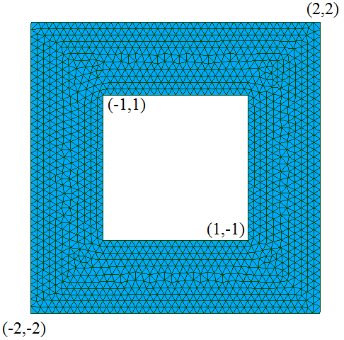
Figure 1: Computational domain: perforated plate.

6.1 Test case (a): Nonlinearity on the solution

We consider the nonlinear parabolic problem (1) with the nonlinear function $\Gamma(\mu,v):=\sin\Big{(}\frac{2\pi\mu}{20}\big{(}\frac{v-u_{0}}{u_{m}-u_{0}}\big{)}^{2}\Big{)}$, with $u_{0}=293$ K (20 ^oC) and $u_{m}=323$ K (50 ^oC). We define $\kappa_{0}=1.05$ m${}^{2}\cdot$K${}^{-2}\cdot$s^-1 and $\phi_{e}=3$ K$\cdot$m$\cdot$s^-1 (these units result from our normalization by the density times the heat capacity). For space discretization, we use a mesh containing $\mathcal{N}=1438$ nodes (see Figure 1). Regarding time discretization, we consider the time interval $I=[0,5]$, the set of discrete times nodes $\mathbb{K}^{\mathrm{tr}}=\{1,\cdots,50\}$, and a constant time step $\Delta t^{k}=0.1$ s for all $k\in\mathbb{K}^{\mathrm{tr}}$. Finally, we consider the parameter interval $\mathcal{P}=[1,20]$, the training set $\mathcal{P}^{\mathrm{tr}}=\{1,\cdots,20\}$, and we use the larger set $\{0.25i\ |\ 0\leq i\leq 80\}$ to verify our numerical results. In Figure 2, we show the HF temperature profiles over the perforated plate at two different times and for two different parameter values. We can see that, as the simulation time increases, the temperature is, overall, higher for larger values of the parameter $\mu$ than for smaller values. Also, for larger values of $\mu$, the temperature variation tends to be less uniform over the plate than for smaller values of $\mu$.

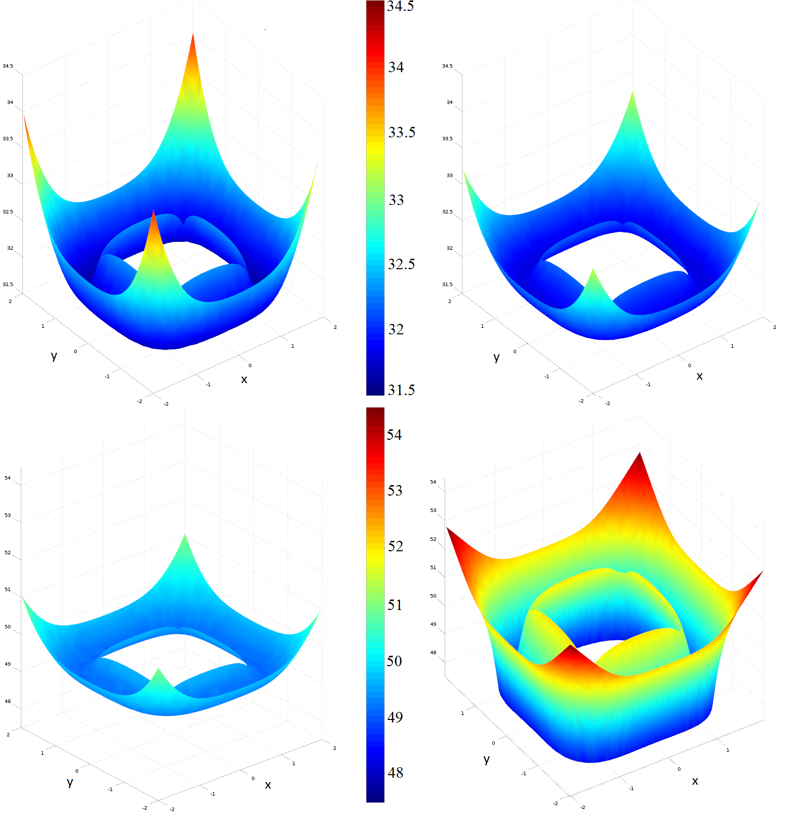
Figure 2: Test case (a): HF solutions for the parameter values $\mu=1$ (left) and $\mu=18$ (right) at $t=2$ s (top) and $t=5$ s (bottom).

$m$	$1$	$2$	$6$	$14$	$15$	$20$	$25$
$\|r_{m}\|_{\ell^{\infty}(\Omega^{\mathrm{tr}})}$	$2.0$	$8.1\mathrm{E}{-1}$	$1.1\mathrm{E}{-1}$	$5.2\mathrm{E}{-3}$	$2.6\mathrm{E}{-3}$	$1.1\mathrm{E}{-3}$	$1.6\mathrm{E}{-4}$

Table 1: Test case (a): Evolution of the standard EIM error. $m$ is the rank of the EIM approximation.

During the standard offline stage, we perform $P=20$ HF computations. Knowing that $K=50$, the set $\mathcal{S}$ (Algorithm 2, line 2) contains $1020$ fields, each consisting of $\mathcal{N}=1438$ nodal values. Applying the POD in a progressive manner (see Algorithm 3 with the parameters enumerated using increasing values) based on the $H^{1}$-norm and a truncation threshold $\epsilon_{\textsc{pod}}=10^{-3}$, we obtain $N=6$ RB functions. Afterwards, we perform the standard EIM algorithm whose convergence is reported in Table 1. For $\epsilon_{\textsc{eim}}=5\cdot 10^{-2}$, the final rank of the EIM approximation is $M=8$, whereas for $\epsilon_{\textsc{eim}}=10^{-3}$, the final rank of the EIM approximation is $M=15$.

$\qquad m$		$1$	$2$	$3$	$4$	$5$	$6$	$7$	$8$	$9$	$10$	$11$	$12$	$13$
PREIM	$\bar{\mu}$	$1$	$20$	$20$	$20$	$20$	$20$	$20$	$20$	$16$	$20$	$20$	$18$	$20$
	$\mu$	$1$	$20$	$20$	$20$	$20$	$18$	$20$	$20$	$16$	$20$	$20$	$18$	$20$
	$k$	$50$	$45$	$48$	$50$	$43$	$42$	$39$	$46$	$50$	$49$	$33$	$50$	$47$

Table 2: Test case (a): Selected parameters and time nodes in PREIM. The gray cells correspond to a new parameter selection and, therefore, to a new HF computation.

We now investigate PREIM, which we first run with thresholds $\epsilon_{\textsc{pod}}=10^{-3}$ and $\epsilon_{\textsc{eim}}=5\cdot 10^{-2}$. Table 2 shows the selected parameters and discrete time nodes at each stage of PREIM. We can make two important observations from this table. First, after 13 iterations, PREIM has only selected four different parameter values, and has therefore computed only four HF trajectories (the iterations for which a new parameter value is selected are indicated in gray in Table 2). In the other $9$ out of the 13 iterations, a different time snapshot of an already existing HF trajectory has been selected. Second, by comparing the lines in Table 2 related to $\mu$ and $\bar{\mu}$, we can see that a parameter re-selection happened at iteration $m=7$.

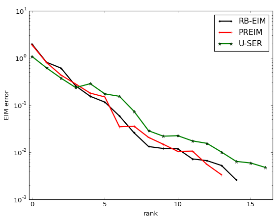
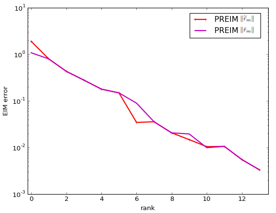
Figure 3: Test case (a): EIM approximation error as a function of $m$ for $\epsilon_{\textsc{pod}}=10^{-3}$ and $\epsilon_{\textsc{eim}}=5\cdot 10^{-2}$. Left: Errors for the standard RB-EIM procedure, PREIM, and U-SER. Right: Errors $\|\widetilde{r}_{m}\|_{\ell^{\infty}(\Omega^{\mathrm{tr}})}$ and $\|\bar{r}_{m}\|_{\ell^{\infty}(\Omega^{\mathrm{tr}})}$ for PREIM.

The left panel of Figure 3 displays the error on the approximation of the nonlinear function $\Gamma$ for the standard RB-EIM procedure and for PREIM as a function of the iteration number $m$ (the additional curve concerning U-SER will be commented afterwards), i.e., we plot $\|\bar{r}_{m}\|_{\ell^{\infty}(\Omega^{\mathrm{tr}})}$ (line 4 of Algorithm 5) and $\|\widetilde{r}_{m}\|_{\ell^{\infty}(\Omega^{\mathrm{tr}})}$ (line 11 of Algorithm 5) as a function of $m$, see (22). We can see that the quality of the approximation of the nonlinearity is almost the same for PREIM as for the standard RB-EIM procedure; yet, the former achieves this accuracy by computing 20% of the HF trajectories computed by the latter (4 instead of 20 HF trajectories). The right panel of Figure 3 shows the values of $\|\widetilde{r}_{m}\|_{\ell^{\infty}(\Omega^{\mathrm{tr}})}$ and $\|\bar{r}_{m}\|_{\ell^{\infty}(\Omega^{\mathrm{tr}})}$ as a function of $m$. The two quantities differ when the parameter $\mu_{m}$ in line 3 of Algorithm 5 is not in the set $\mathcal{P}^{\mathrm{HF}}_{m-1}$ so that $\|\widetilde{r}_{m}\|_{\ell^{\infty}(\Omega^{\mathrm{tr}})}$ is computed using a RB approximation whereas $\|\bar{r}_{m}\|_{\ell^{\infty}(\Omega^{\mathrm{tr}})}$ results from a HF trajectory. Discarding the initialization, this happens for $m\in\{6,9,10\}$. The fact that $\|\widetilde{r}_{m}\|_{\ell^{\infty}(\Omega^{\mathrm{tr}})}$ and $\|\bar{r}_{m}\|_{\ell^{\infty}(\Omega^{\mathrm{tr}})}$ take rather close values indicates that the RB provides an accurate approximation of the HF trajectory.

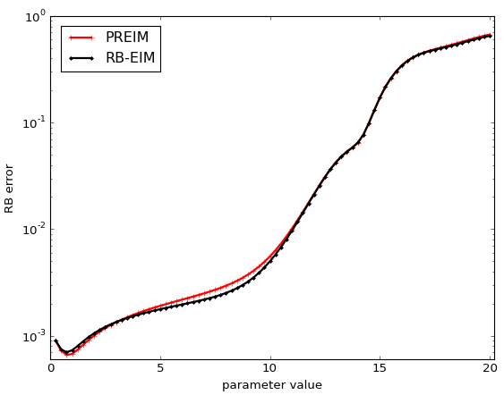
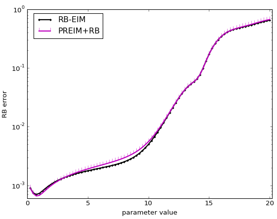
Figure 4: Test case (a): RB approximation error $\|u_{\mu}-\hat{u}_{\mu}\|_{\ell^{2}(I^{\mathrm{tr}};H^{1}(\Omega^{\mathrm{tr}}))}$ for $\epsilon_{\textsc{pod}}=10^{-3}$ and $\epsilon_{\textsc{eim}}=5\cdot 10^{-2}$.

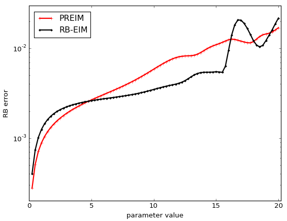
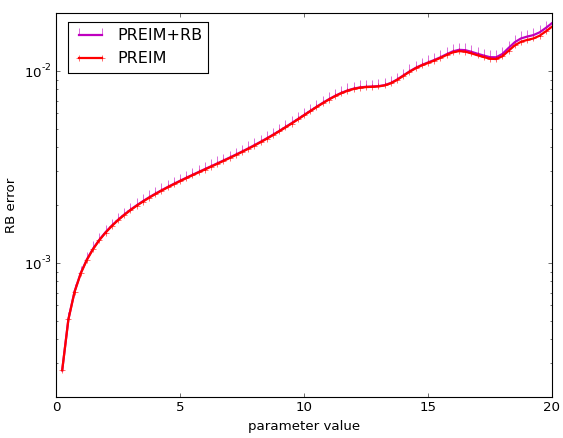
Figure 5: Test case (a): RB approximation error $\|u_{\mu}-\hat{u}_{\mu}\|_{\ell^{2}(I^{\mathrm{tr}};H^{1}(\Omega^{\mathrm{tr}}))}$ for $\epsilon_{\textsc{pod}}=10^{-5}$ and $\epsilon_{\textsc{eim}}=5\cdot 10^{-3}$.

The left panel of Figure 4 compares the space-time errors (measured using the $\ell^{2}$-norm in time and the $H^{1}$-norm in space) on the trajectories produced by the standard RB-EIM and the PREIM procedures for the whole parameter range. The error is generically denoted $\|u_{\mu}-\hat{u}_{\mu}\|_{\ell^{2}(I^{\mathrm{tr}};H^{1}(\Omega^{\mathrm{tr}}))}$. We observe an excellent agreement over the whole parameter range. In the right panel of Figure 4, we also consider the space-time errors on the trajectories produced using the approximation of the nonlinearity resulting from PREIM with the RB resulting from the standard algorithm. We do not observe any significant change with respect to the left panel, which indicates that the dominant error component is that associated with the approximation of the nonlinearity. We consider the tighter couple of thresholds $\epsilon_{\textsc{pod}}=10^{-5}$ and $\epsilon_{\textsc{eim}}=5\cdot 10^{-3}$ in Figure 5. Here, we can observe some differences in the errors produced by the standard RB-EIM and PREIM procedures, although both errors remain comparable and reach similar maximum values over the parameter range. While the standard procedure is slightly more accurate for most parameter values, the conclusion is reversed for some other values. Moreover, the curves on the right panel of Figure 5 corroborate the fact that once again, the dominant error component is that associated with the approximation of the nonlinearity.

$\qquad m$		$1$	$2$	$3$	$4$	$5$	$6$	$7$	$8$	$9$	$10$	$11$	$12$	$13$
U-SER	$\mu$	$1$	$20$	$20$	$20$	$16$	$20$	$19$	$20$	$20$	$19$	$17$	$20$	$19$
	$k$	$50$	$49$	$50$	$46$	$42$	$49$	$44$	$39$	$50$	$49$	$48$	$47$	$50$
PREIM-NR	$\mu$	$1$	$20$	$20$	$20$	$20$	$16$	$20$	$20$	$20$	$20$	$20$	$17$	$19$
	$k$	$50$	$47$	$50$	$46$	$42$	$49$	$48$	$46$	$39$	$50$	$45$	$50$	$50$

Table 3: Test case (a): Selected parameters and time nodes in U-SER and PREIM-NR. The gray cells correspond to a new parameter selection and, therefore, to a new HF computation.

Let us further explore the PREIM algorithm by comparing it to its variants U-SER and PREIM-NR introduced in Remark 5. Table 3 reports the selected parameters and time nodes in U-SER and PREIM-NR (compare with Table 2 for PREIM). Both U-SER and PREIM-NR need to compute five HF trajectories, which is only 25% of those needed with the standard RB-EIM procedure, but this is still one more HF trajectory than with PREIM. One difference between U-SER and PREIM-NR is that new parameters are selected earlier with U-SER. Interestingly, after 13 iterations, U-SER and PREIM-NR have selected the same five parameters. Another interesting observation is that U-SER actually selects the same couple $(\mu,k)$ twice (this happens for $m=2$ and $m=6$); this can be interpreted by observing that owing to the improvement of the RB using HF trajectories between iterations $m=2$ and $m=6$, the algorithm detects the need to improve the approximation of the nonlinearity by using the same pair $(\mu,k)$. The same observation can be made for PREIM-NR (this happens for $m=4$ and $m=8$). We emphasize that re-selecting the same pair $(\mu,k)$ is not possible within PREIM since the selection is based on HF trajectories. The left panel of Figure 3 displays the error on the approximation of the nonlinear function $\Gamma$ obtained with U-SER and compares it to the error obtained with the standard RB-EIM and PREIM procedures that were already discussed. The U-SER error is evaluated as $\sup_{(\mu,k)\in\mathcal{P}^{\mathrm{tr}}\times\overline{\mathbb{K}}^{\mathrm{tr}}}\|\Gamma(\mu,\hat{u}^{k}_{\mu}(\cdot))-\overline{\gamma}_{[\mathcal{P}_{m}^{\textsc{HF}},\mathcal{X}_{m},\mathcal{Q}_{m}]}^{m}(\mu,k,\cdot)\|_{\ell^{\infty}(\Omega^{\mathrm{tr}})}$. We observe that the approximation of the nonlinearity is somewhat less sharp with U-SER than with PREIM. Figure 6 reports the space-time errors (measured using the $\ell^{2}$-norm in time and the $H^{1}$-norm in space) on the trajectories produced by PREIM and U-SER for the whole parameter range. We observe that the U-SER error is always larger, sometimes up to a factor of five, but for the larger parameter values which produce the larger errors, the quality of the results produced by PREIM and U-SER remains comparable.

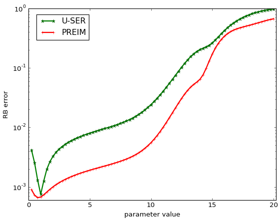
Figure 6: Test case (a): RB approximation error $\|u_{\mu}-\hat{u}_{\mu}\|_{\ell^{2}(I^{\mathrm{tr}};H^{1}(\Omega^{\mathrm{tr}}))}$ for $\epsilon_{\textsc{pod}}=10^{-3}$ and $\epsilon_{\textsc{eim}}=5\cdot 10^{-2}$.

	RB-EIM	PREIM	U-SER
HF computations	$99\%$	$20.0\%$	$25.0\%$
greedy runtime	$1\%$	$1.5\%$	$2.3\%$
Total runtime	$100\%$	$21.5\%$	$26.3\%$

Table 4: Test case (a): Runtime measurements.

Finally, we provide an assessment of the runtimes in Table 4. We can see that for the standard RB-EIM procedure, the computation of the HF trajectories dominates the cost of the offline phase. For both PREIM and U-SER, the cost of these HF computations is substantially reduced. At the same time, the cost of the greedy algorithm (which includes the construction of the EIM and of the RB) is increased by 50% with respect to the standard RB-EIM procedure. However, the impact on the total runtime is marginal.

6.2 Test case (b): Nonlinearity on the partial derivatives

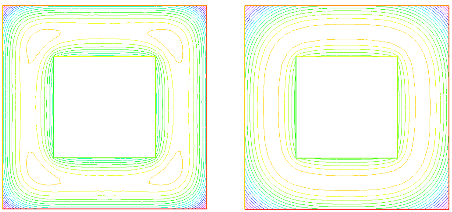
Figure 7: Test case (b): HF solutions for the parameter values $\mu=1$ at $t=1$ s (left, values from 20.2 to 22.1) and at $t=2.5$ s (right, values from 34.5 to 37.3).

We consider the nonlinear parabolic problem (1) with the nonlinear function $\Gamma(\mu,u):=\sin\Big{(}\omega\mu\big{(}({\frac{\partial u}{\partial x}})^{2}+({\frac{\partial u}{\partial y}})^{2}\big{)}\Big{)}^{2}$, where $\omega=6.25\cdot 10^{-3}$. We define $u_{0}=293$ K (20 ^oC), $\kappa_{0}=1$ m${}^{2}\cdot$K${}^{-2}\cdot$s^-1 and $\phi_{e}=3$ K$\cdot$m$\cdot$s^-1 (these units result from our normalization by the density times the heat capacity). For the space discretization, we use a mesh containing $\mathcal{N}=1429$ nodes. Regarding time discretization, we consider the time interval $I=[0,2.5]$, the set of discrete times nodes $\mathbb{K}^{\mathrm{tr}}=\{1,\ldots,50\}$, and a constant time step $\Delta t^{k}=0.05$ s for all $k\in\mathbb{K}^{\mathrm{tr}}$. Finally, we consider the parameter interval $\mathcal{P}=[1,40]$ and the training set $\mathcal{P}^{\mathrm{tr}}=\{1,\ldots,40\}$. In Figure 7, we show the temperature isovalues over the perforated plate at two different times for $\mu=1$. We can observe different boundary layers depending on the time (the same observation can be made by varying the parameter value).

$p$	$1$	$2$	$3$	$8$	$20$	$23$	$24$	$26$	$32$	$33$	$36$	$37$	$39$	$40$
RB size	$3$	$4$	$5$	$6$	$7$	$8$	$9$	$10$	$11$	$12$	$13$	$14$	$15$	$15$

Table 5: Test case (b): Size of the reduced basis in the standard algorithm with $\epsilon_{\textsc{pod}}=5\cdot 10^{-2}$.

$m$	$2$	$10$	$13$	$20$	$30$	$36$	$37$	$79$	$96$	$144$
$\|r_{m}\|_{\ell^{\infty}(\Omega^{\rm tr})}$	$1.6$	$1.3$	$9.7{\rm E}{-1}$	$4.7{\rm E}{-1}$	$1.7{\rm E}{-1}$	$1.2{\rm E}{-1}$	$8.0{\rm E}{-2}$	$9.1{\rm E}{-3}$	$4.6{\rm E}{-3}$	$9.4{\rm E}{-4}$

Table 6: Test case (b): Evolution of the standard EIM error. $m$ is the rank of the EIM approximation and $\|r_{m}\|_{\ell^{\infty}(\Omega^{\mathrm{tr}})}$ is the residual norm in (18).

During the standard offline stage, we perform $P=40$ HF computations. Knowing that $K=50$, the set $\mathcal{S}$ (Algorithm 2, line 2) contains $2040$ fields, each consisting of $\mathcal{N}=1429$ nodal values. Applying Algorithm 3 based on the $H^{1}$-norm, a truncation threshold $\epsilon_{\textsc{pod}}=5\cdot 10^{-2}$, and parameters enumerated with increasing values, we obtain $N=15$ RB functions. Table 5 shows the dimension of the RB space as a function of the enumeration index $p$. Table 6 shows the evolution of the error on the nonlinearity within the standard EIM. The fact that the nonlinearity depends on the partial derivatives of the solution challenges the EIM; indeed, the error decay is not as fast as in the previous test case. This observation is corroborated by the fact that the functions $(q_{j})_{1\leq j\leq M}$ all look quite different.

$m$ $1$ $2$ $3$ $4$ $5$ $6$ $7$ $8$ $9$ $\bar{\mu}$ $21$ $8$ $21$ $8$ $21$ $21$ $21$ $8$ $9$ $\mu$ $21$ $8$ $21$ $8$ $21$ $21$ $21$ $8$ $9$ $k$ $2$ $5$ $3$ $2$ $50$ $4$ $49$ $3$ $4$

$m$ $1$ $2$ $3$ $4$ $5$ $6$ $7$ $8$ $9$ $10$ $11$ $12$ $13$ $14$ $15$ $16$ $17$ $18$ $19$ $20$ $\bar{\mu}$ $21$ $21$ $21$ $8$ $21$ $21$ $21$ $8$ $9$ $21$ $9$ $21$ $9$ $9$ $9$ $6$ $21$ $21$ $40$ $40$ $\mu$ $21$ $8$ $21$ $8$ $21$ $21$ $21$ $8$ $9$ $21$ $9$ $7$ $6$ $9$ $9$ $5$ $4$ $3$ $40$ $40$ $k$ $2$ $5$ $3$ $2$ $50$ $4$ $49$ $3$ $4$ $10$ $50$ $25$ $49$ $5$ $10$ $4$ $6$ $9$ $15$ $40$

Table 7: Test case (b): Selected parameters and time nodes in PREIM for $\epsilon_{\textsc{eim}}=10^{-1}$ (top) and $\epsilon_{\textsc{eim}}=10^{-3}$ (bottom). The gray cells correspond to a new parameter selection and, therefore, to a new HF computation.

$m$	$1$	$2$	$9$	$17$	$18$	$20$
RB size	$5$	$6$	$6$	$7$	$9$	$9$

Table 8: Test case (b): Size of RB generated within PREIM for $\epsilon_{\textsc{pod}}=5\cdot 10^{-2}$; for $\epsilon_{\textsc{eim}}=10^{-1}$, one stops at $m=9$, and for $\epsilon_{\textsc{eim}}=10^{-3}$, one stops at $m=20$.

We now investigate the performance of PREIM, which we run with thresholds $\epsilon_{\textsc{pod}}=5\cdot 10^{-2}$ and either $\epsilon_{\textsc{eim}}=10^{-1}$ or $\epsilon_{\textsc{eim}}=10^{-3}$. Table 7 shows the selected parameters and time nodes at each iteration. For $\epsilon_{\textsc{eim}}=10^{-1}$, PREIM performs 9 iterations, and three parameters are selected for HF computations, whereas for $\epsilon_{\textsc{eim}}=10^{-3}$, PREIM performs $11$ further iterations and six more HF computations to reach the requested threshold. Moreover, the evolution of the size of the reduced basis within PREIM is shown in Table 8. As can be noticed, the approximation of the nonlinearity requires more computational effort than that of the solution manifold.

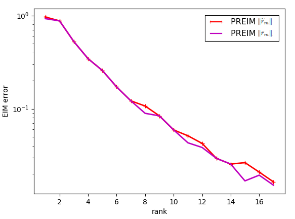
Figure 8: Test case (b): EIM approximation errors $\|\widetilde{r}_{m}\|_{\ell^{\infty}(\Omega^{\mathrm{tr}})}$ and $\|\bar{r}_{m}\|_{\ell^{\infty}(\Omega^{\mathrm{tr}})}$ as a function of $m$ for PREIM with $\epsilon_{\textsc{pod}}=5\cdot 10^{-2}$ and $\epsilon_{\textsc{eim}}=10^{-3}$.

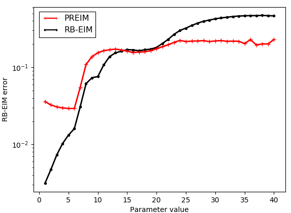
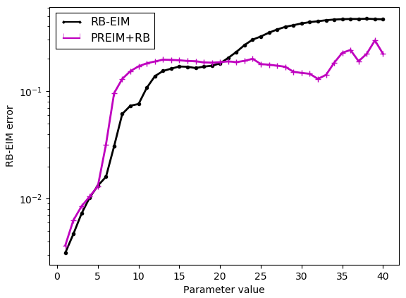
Figure 9: Test case (b): RB approximation error $\|u_{\mu}-\hat{u}_{\mu}\|_{\ell^{2}(I^{\mathrm{tr}};H^{1}(\Omega^{\mathrm{tr}}))}$ for $\epsilon_{\textsc{pod}}=5\cdot 10^{-2}$ and $\epsilon_{\textsc{eim}}=10^{-3}$.

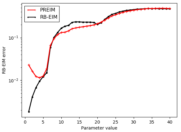
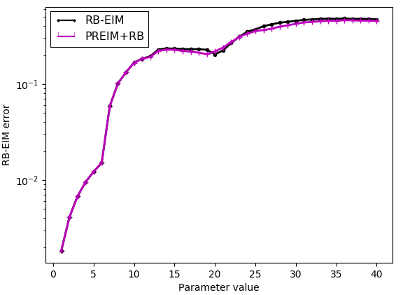
Figure 10: Test case (b): RB approximation error $\|u_{\mu}-\hat{u}_{\mu}\|_{\ell^{2}(I^{\mathrm{tr}};H^{1}(\Omega^{\mathrm{tr}}))}$ for $\epsilon_{\textsc{pod}}=2.5\cdot 10^{-2}$ and $\epsilon_{\textsc{eim}}=10^{-4}$.

Figure 8 shows the decrease of the EIM approximation error on the nonlinearity for PREIM with $\epsilon_{\textsc{pod}}=5\cdot 10^{-2}$ and $\epsilon_{\textsc{eim}}=10^{-3}$. We observe that each time a new HF trajectory is computed, i.e., whenever the quantities $\|\widetilde{r}_{m}\|_{\ell^{\infty}(\Omega^{\mathrm{tr}})}$ and $\|\bar{r}_{m}\|_{\ell^{\infty}(\Omega^{\mathrm{tr}})}$ differ, the difference is actually rather small, thereby confirming the already accurate approximation of the nonlinearity by the RB solutions in PREIM. The left panel of Figure 9 illustrates the space-time errors (measured in the $\ell^{2}(I^{\mathrm{tr}};H^{1}(\Omega^{\mathrm{tr}}))$-norm) on the trajectories produced by the standard RB-EIM and the PREIM procedures for the whole parameter range. We observe that for lower parameter values, PREIM delivers somewhat less accurate results, whereas the conclusion is reversed for higher parameter values. Altogether, both errors stay within comparable upper bounds. The right panel of Figure 9 shows that the error component associated with the approximation of the nonlinearity is still the dominant one, except for the parameter range $[1,5]$ where the RB from the standard algorithm helps improve the error. Incidentally, we observe that these smaller values of the parameter were not selected within PREIM for approximating the nonlinearity. Finally, Figure 10 shows the same results for the tighter thresholds $\epsilon_{\textsc{pod}}=5\cdot 10^{-2}$ and $\epsilon_{\textsc{eim}}=10^{-4}$. Here, $14$ HF computations and $100$ PREIM iterations were needed. We can see that the PREIM error closely matches that of the standard RB-EIM procedure.

7 Conclusion and perspectives

In this work, we have devised a new methodology, called PREIM, that allows one to diminish the offline expenses incurred in the nonlinear RB method applied to unsteady nonlinear PDEs, as long as the computation of high-fidelity trajectories is the dominant part of the offline cost. Numerical tests on two-dimensional nonlinear heat transfer problems with nonlinear thermal conductivities have illustrated the computational efficiency and the accuracy of the algorithm. In addition, the application of PREIM to an industrial test case of a three-dimensional flow-regulation valve is ongoing.

Acknowledgments

This work is partially supported by Electricité De France (EDF) and a CIFRE PhD fellowship from ANRT. The authors are grateful to G. Blatman (EDF) and M. Abbas (EDF) for stimulating discussions and for their help on code_aster. The authors are thankful to the two anonymous reviewers for their valuable comments.

Appendix A Proper Orthogonal Decomposition

The goal of this appendix is to briefly describe the procedure associated with the notation

$$(\theta_{1},\ldots,\theta_{N})=\mathrm{POD}(\mathcal{S},\epsilon_{\textsc{pod}}),$$ (27)

which is used in Algorithms 3, 4, and 6, where $\mathcal{S}=(v_{1},\ldots,v_{R})$ is composed of $R\geq 1$ functions in the space $X$ and $\epsilon_{\textsc{pod}}$ is a user-prescribed tolerance. For simplicity, we adopt an algebraic description, and we refer the reader to [2] for further insight. Let $(\varrho_{1},\ldots,\varrho_{\mathcal{N}})$ be a basis of $X$ where $\mbox{\rm dim}(X)=\mathcal{N}$. For a function $w\in X$, we denote by $\mathbf{w}:=(w_{j})_{1\leq j\leq\mathcal{N}}$ its coordinate vector in $\mathbb{R}^{\mathcal{N}}$, so that $w=\sum_{j=1}^{\mathcal{N}}w_{j}\varrho_{j}$. The algebraic counterpart of (27) is that we are given $R$ vectors forming the rectangular matrix $\mathbf{S}:=(\mathbf{v}_{1},\ldots,\mathbf{v}_{R})\in\mathbb{R}^{\mathcal{N}\times R}$, and we are looking for $N$ vectors forming the rectangular matrix $\bm{\Theta}:=(\bm{\theta}_{1},\ldots,\bm{\theta}_{N})\in\mathbb{R}^{\mathcal{N}\times N}$. The vectors $(\bm{\theta}_{1},\ldots,\bm{\theta}_{N})$ are to be orthonormal with respect to the Gram matrix of the inner product in $X$. In the present setting, we consider the Gram matrix $\mathbf{C}^{\mathcal{N}}\in\mathbb{R}^{\mathcal{N}\times\mathcal{N}}$ such that

$$\mathbf{C}^{\mathcal{N}}=\Big{(}m(\varrho_{n},\varrho_{p})+\eta a_{0}(\varrho_{n},\varrho_{p})\Big{)}_{1\leq p,n\leq\mathcal{N}},$$ (28)

where $\eta>0$ is a user-prescribed weight and the bilinear forms $m$ and $a_{0}$ are defined in (3). Thus, we want to have $\bm{\theta}_{n}^{\mathrm{T}}\mathbf{C}^{\mathcal{N}}\bm{\theta}_{p}=\delta_{n,p}$, the Kronecker delta, for all $n,p\in\{1,\ldots,N\}$.

Let us set $\mathbf{T}:=(\mathbf{C}^{\mathcal{N}})^{\frac{1}{2}}\mathbf{S}\in\mathbb{R}^{\mathcal{N}\times R}$ and consider the integer $D=\min(\mathcal{N},R)$ (in most situations, we have $D=R$ and $D\ll\mathcal{N}$). Computing the Singular Value Decomposition [16] of the matrix $\mathbf{T}$, we obtain the real numbers $\sigma_{1}\geq\sigma_{2}\geq\cdots\geq\sigma_{D}\geq 0$, the orthonormal family of column vectors $(\bm{\xi}_{n})_{1\leq n\leq D}\in(\mathbb{R}^{\mathcal{N}})^{D}$ (so that $\bm{\xi}_{n}^{\mathrm{T}}\bm{\xi}_{p}=\delta_{p,n}$) and the orthonormal family of column vectors $(\hat{\bm{\psi}}_{n})_{1\leq n\leq D}\in(\mathbb{R}^{R})^{D}$ (so that $\hat{\bm{\psi}}_{n}^{\mathrm{T}}\hat{\bm{\psi}}_{p}=\delta_{p,n}$), and we have

$$\mathbf{T}=\sum_{n=1}^{D}\sigma_{n}\bm{\xi}_{n}\hat{\bm{\psi}}_{n}^{\mathrm{T}}.$$ (29)

From (29), it follows that $\mathbf{T}\hat{\bm{\psi}}_{n}=\sigma_{n}\bm{\xi}_{n}$ and $\mathbf{T}^{\mathrm{T}}\bm{\xi}_{n}=\sigma_{n}\hat{\bm{\psi}}_{n}$ for all $n\in\{1,\ldots,D\}$. The vectors we are looking for are then given by $\bm{\theta}_{n}:=(\mathbf{C}^{\mathcal{N}})^{-\frac{1}{2}}\bm{\xi}_{n}$ for all $n\in\{1,\ldots,N\}$ with $N:=\max\{1\leq n\leq D\ |\ \sigma_{n}\geq\epsilon_{\textsc{POD}}\}$. It is well-known that the $N$-dimensional space spanned by the vectors $(\bm{\theta}_{n})_{1\leq n\leq N}$ minimizes the quantity $\mathop{\inf}_{\mathbf{z}\in\mathbf{Z}_{N}}\sum_{r=1}^{R}(\mathbf{v}_{r}-\mathbf{z})^{\mathrm{T}}\mathbf{C}^{\mathcal{N}}(\mathbf{v}_{r}-\mathbf{z})$ among all the $N$-dimensional subspaces $\mathbf{Z}_{N}$ of $\mathbb{R}^{\mathcal{N}}$. Moreover, we have $\|v-\Pi_{Z_{N}}v\|_{X}\leq\sigma_{N+1}\|v\|_{X}$, for all $v\in\mathcal{S}$.

In practice, when $D=R$, we can avoid the computation of the matrix $(\mathbf{C}^{\mathcal{N}})^{\frac{1}{2}}$ and of its inverse by considering the matrix of smaller dimension $\mathbf{T}^{\mathrm{T}}\mathbf{T}=\mathbf{S}^{\mathrm{T}}\mathbf{C}^{\mathcal{N}}\mathbf{S}\in\mathbb{R}^{R\times R}$. Solving for the eigenvalues of $\mathbf{T}^{\mathrm{T}}\mathbf{T}$, we obtain the vectors $\hat{\bm{\psi}}_{n}$ with associated eigenvalues $\sigma_{n}^{2}$ since we have $\mathbf{T}^{\mathrm{T}}\mathbf{T}\hat{\bm{\psi}}_{n}=\sigma_{n}\mathbf{T}^{\mathrm{T}}\bm{\xi}_{n}=\sigma_{n}^{2}\hat{\bm{\psi}}_{n}$. Then, the vectors $(\bm{\theta}_{n})_{1\leq n\leq N}$ are obtained as $\bm{\theta}_{n}=\left(\mathbf{C}^{\mathcal{N}}\right)^{-\frac{1}{2}}\bm{\xi}_{n}=\frac{1}{\sigma_{n}}\left(\mathbf{C}^{\mathcal{N}}\right)^{-\frac{1}{2}}\mathbf{T}\hat{\bm{\psi}}_{n}=\frac{1}{\sigma_{n}}\mathbf{S}\hat{\bm{\psi}}_{n}.$

References

- [1] M. Barrault, Y. Maday, N. C. Nguyen, and A. T. Patera, An ‘empirical interpolation’ method: application to efficient reduced-basis discretization of partial differential equations, C. R. Math. Acad. Sci. Paris, 339 (2004), pp. 667–672.
- [2] P. Benner, A. Cohen, M. Ohlberger, and K. Willcox, eds., Model Reduction and Approximation, SIAM, Philadelphia, 2017.
- [3] C. Daversin and C. Prud’homme, Simultaneous empirical interpolation and reduced basis method for non-linear problems, C. R. Math. Acad. Sci. Paris, 353 (2015), pp. 1105–1109.
- [4] M. Drohmann, B. Haasdonk, and M. Ohlberger, Reduced basis approximation for nonlinear parametrized evolution equations based on empirical operator interpolation, SIAM J. Sci. Comput., 34 (2012), pp. A937–A969.
- [5] Electricité de France, Finite element , analysis of structures and thermomechanics for studies and research. Open source on www.code-aster.org, 1989–2017.
- [6] A. Ern and J.-L. Guermond, Theory and Practice of Finite Elements, Applied Mathematical Sciences, Springer New York, 2004.
- [7] M. A. Grepl, Certified reduced basis methods for nonaffine linear time-varying and nonlinear parabolic partial differential equations, Math. Models Methods Appl. Sci., 22 (2012), pp. 1150015, 40.
- [8] M. A. Grepl, Y. Maday, N. C. Nguyen, and A. T. Patera, Efficient reduced-basis treatment of nonaffine and nonlinear partial differential equations, M2AN Math. Model. Numer. Anal., 41 (2007), pp. 575–605.
- [9] B. Haasdonk, Convergence rates of the POD-greedy method, ESAIM Math. Model. Numer. Anal., 47 (2013), pp. 859–873.
- [10] F. Hecht, FreeFem++, Third Edition, Version 3.0-1. User’s Manual, LJLL, University Paris VI.
- [11] J. S. Hesthaven, G. Rozza, and B. Stamm, Certified reduced basis methods for parametrized partial differential equations, SpringerBriefs in Mathematics, Springer, Cham; BCAM Basque Center for Applied Mathematics, Bilbao, 2016. BCAM SpringerBriefs.
- [12] M. Hinze and S. Volkwein, Proper orthogonal decomposition surrogate models for nonlinear dynamical systems: error estimates and suboptimal control, in Dimension reduction of large-scale systems, vol. 45 of Lect. Notes Comput. Sci. Eng., Springer, Berlin, 2005, pp. 261–306.
- [13] K. Kunisch and S. Volkwein, Galerkin proper orthogonal decomposition methods for parabolic problems, Numer. Math., 90 (2001), pp. 117–148.
- [14] L. Machiels, Y. Maday, I. B. Oliveira, A. T. Patera, and D. V. Rovas, Output bounds for reduced-basis approximations of symmetric positive definite eigenvalue problems, C. R. Acad. Sci. Paris Sér. I Math., 331 (2000), pp. 153–158.
- [15] Y. Maday, N. C. Nguyen, A. T. Patera, and G. S. H. Pau, A general multipurpose interpolation procedure: the magic points, Commun. Pure Appl. Anal., 8 (2009), pp. 383–404.
- [16] B. Noble and J. W. Daniel, Applied Linear Algebra, Prentice-Hall, 3rd ed., 1988.
- [17] C. Prud’Homme, D. V. Rovas, K. Veroy, L. Machiels, Y. Maday, A. T. Patera, and G. Turinici, Reliable Real-Time Solution of Parametrized Partial Differential Equations: Reduced-Basis Output Bound Methods, Journal of Fluids Engineering, 124 (2001), pp. 70–80.
- [18] A. Quarteroni, A. Manzoni, and F. Negri, Reduced basis methods for partial differential equations, La Matematica per il 3+2, Springer International Publishing, 2016.
- [19] D. V. Rovas, L. Machiels, and Y. Maday, Reduced-basis output bound methods for parabolic problems, IMA J. Numer. Anal., 26 (2006), pp. 423–445.
- [20] K. Urban and B. Wieland, Affine decompositions of parametric stochastic processes for application within reduced basis methods, IFAC Proceedings Volumes, 45 (2012), pp. 716–721.