Time-independent Green’s Function

of a Quantum Simple Harmonic Oscillator System and

Solutions with Additional Generic Delta-Function Potentials

Chun-Khiang Chua, Yu-Tsai Liu, Gwo-Guang Wong

Department of Physics and Chung Yuan Center for High Energy Physics,

Chung Yuan Christian University,

Chung-Li, Taoyuan, Taiwan 32023, Republic of China

Abstract

The one-dimensional time-independent Green’s function $G_{0}$ of a quantum simple harmonic oscillator system ($V_{0}(x)=m\omega^{2}x^{2}/2$) can be obtained by solving the equation directly. It has a compact expression, which gives correct eigenvalues and eigenfunctions easily. The Green’s function $G$ with an additional delta-function potential can be obtained readily. The same technics of solving the Green’s function $G_{0}$ can be used to solve the eigenvalue problem of the simple harmonic oscillator with an generic delta-function potential at an arbitrary site, i.e. $V_{1}(x)\propto\delta(x-a)$. The Wronskians play an important and interesting role in the above studies. Furthermore, the approach can be easily generalized to solve the quantum system of a simple harmonic oscillator with two or more generic delta-function potentials. We give the solutions of the case with two additional delta-functions for illustration.

I Introduction

The one-dimensional quantum simple harmonic oscillator (SHO) has become an indispensable material on the textbooks of quantum mechanics (for example, see Gasiorowicz ) and widely used in many different physics and chemistry fields AA ; BB . It is one of the most important model systems in quantum mechanics since any binding potential can usually be approximated as a harmonic potential at the vicinity of a stable equilibrium point. It can be applied to the vibration of diatomic molecule, the Hooke’s atom KS , the vibrations of atoms in a solid Franz2008 , the quantum Hall effect Laughlin1981 , the atoms in optical traps Yannouleas1999 and so on. The Schrödinger differential equation for a quantum SHO system can be analytically solved using either the Frobenius method Lebedev with an infinite series expansion or the algebra method Griffiths with the creation and annihilation operators to solve the eigenfunctions and the corresponding eigenvalues. Hence SHO is naturally to have research as well as pedagogical values. 

SHO is always a topic of interest. There are much to be investigated on this old, simple but important subject. For example, it has been shown that the one-dimensional quantum harmonic oscillator problem is examined via the Laplace transform method. The stationary states are determined by requiring definite parity and good behaviour of the eigenfunction at the origin and at infinity Pimentel de Castro . Recently, in Ref. Nogueira de Castro , the exponential Fourier approach in the literature to the one-dimensional quantum harmonic oscillator problem is revised and criticized. The problem is revisited via the Fourier sine and cosine transform method and the stationary states are properly determined by requiring definite parity and square-integrable eigenfunctions Nogueira de Castro .

Ref Viana-Gomes pointed out that an additional boundary condition neglected in the usual quantum mechanics textbooks should be imposed. It was shown that the following wave function satisfies the boundary condition and the Schrödinger equation of SHO ($V(x)=m\omega^{2}x^{2}/2$) for $x\neq 0$,

$$u_{\nu}(x)=Ae^{-\frac{1}{2}(\alpha x)^{2}}U\left(-\frac{\nu}{2},\frac{1}{2},(\alpha x)^{2}\right),$$ (1)

where $\alpha=\sqrt{m\omega/\hbar}$ and $U(a,b,x)$ is the Tricomi’s (confluent hypergeometric) function. Requiring the derivative of the wave function be continuous at $x=0$, as implicated by the Schrödinger equation around $x=0$, gives $\nu=n=0,1,2,\cdots$ and

$$u_{\nu}(x)=u_{n}(x)\propto e^{-\frac{1}{2}(\alpha x)^{2}}H_{n}(\alpha x).$$ (2)

For non-integer $\nu$ the derivative of the wave function is discontinuous, as a byproduct it can be used to constructed the solution of the Schrödinger equation of SHO with a delta-function potential at the origin. In ref. Patil a harmonic oscillator with a $\delta(x)$ potential is analysed and compact expressions for the energy eigenvalues of the even parity states are also obtained. However, these authors only considered the case of SHO with a delta-function potential located at the origin.

In this work, we use Green’s function to solve the eigenvalue problem of a quantum SHO system in a new way, which is not given in any textbook and in the literature. For an introduction of Green’s functions in quantum mechanics, one is referred to ref. Economou ; Sakurai . The important role of Wronskian played in obtaining the energy eigenvalues and eigenfunctions will be shown and hopefully be appreciated. Using the very same technics, one can easily solve the eigenvalue problem for a quantum SHO with one (two) additional delta-function potential(s) at an arbitrary site (arbitrary sites) directly from solving the Schrödinger equation. In this way, we can have better understanding on the quantum SHO system with or without delta-function potentials. Some of our results can be found in YTLiu , which is prepared by one of the authors (YTL) based on a preliminary version of the present work.

This paper is organized as follows. In Sec. II and III, we derive the time-independent Green’s functions for the quantum systems of pure SHO, and SHO with a generic delta-function potential at an arbitrary site, respectively. From the poles of these Green’s functions, we obtain the eigenvalues and eigenfunctions corresponding to the related quantum systems. In Sec IV and V, we derive the wave functions directly from the Schrödinger equation for the quantum systems of SHO with one and two generic delta-function(s), respectively. Sec. IV is the conclusion.

II Time-independent Green’s function of a quantum simple harmonic oscillator

The time-independent Green’s function of a quantum simple harmonic oscillator satisfies the following equation:

$$\left(-\frac{\hbar^{2}}{2m}\frac{\partial^{2}}{\partial x^{2}}+\frac{1}{2}m\omega^{2}x^{2}-E\right)G_{0}(x,y;E)=\delta(x-y).$$ (3)

By changing the variables,

$$\alpha\equiv\sqrt{\frac{m\omega}{\hbar}},\quad\varepsilon\equiv\frac{m}{\alpha^{2}\hbar^{2}}E=\frac{E}{\hbar\omega},$$ (4)

the original equation can be expressed as

$$\left(\frac{\partial^{2}}{\partial x^{2}}-\alpha^{4}x^{2}+2\alpha^{2}\varepsilon\right)G_{0}(x,y;E)=-\frac{2m}{\hbar^{2}}\delta(x-y).$$ (5)

The Green’s function needs to satisfy the following boundary conditions:

$$\lim_{x\to\pm\infty}G_{0}(x,y;E)=0,$$ (6)

and the matching conditions around $x=y$:

$$G_{0}(x = y^{+},y,E)=G_{0}(x=y^{-},y;E),$$ (7)

$$\Delta G^{\prime}_{0}(y;E)\equiv\frac{\partial}{\partial x}G_{0}(x = y^{+},y;E)-\frac{\partial}{\partial x}G_{0}(x=y^{-},y;E)=-\frac{2m}{\hbar^{2}},$$ (8)

where the last equation is obtained from integrating both sides of Eq. (5) around $x=y$. The standard procedure of solving $G_{0}$ is assuming that it takes the following form Jackson :

$$G_{0}(x,y;E)=Af_{<}\left(\min(x,y)\right)f_{>}\left(\max(x,y)\right),$$ (9)

where $f_{<}(x)$ and $f_{>}(x)$ satisfy

$$\left(\frac{\partial^{2}}{\partial x^{2}}-\alpha^{2}x^{2}+2\alpha^{2}\varepsilon\right)f_{<,>}(x)=0,$$ (10)

with the boundary conditions

$$\lim_{x\to-\infty}f_{<}(x)=0,\quad\lim_{x\to\infty}f_{>}(x)=0,$$ (11)

$f_{>}(x)$ can be expressed as combinations of two linearly independent solutions Lebedev :

$$f_{>}(x)=c_{1}e^{-\alpha^{2}x^{2}/2}H_{\nu}(\alpha x)+c_{2}e^{\alpha^{2}x^{2}/2}H_{-\nu-1}(i\alpha x),$$ (12)

with

$$\nu\equiv\varepsilon-\frac{1}{2}.$$ (13)

From Eq. (10), we see that if $f(x)$ is a solution, $f(-x)$ is also a solution. It is convenient to use

$$f_{<}(x)=c_{3}e^{-\alpha^{2}x^{2}/2}H_{\nu}(-\alpha x)+c_{4}e^{\alpha^{2}x^{2}/2}H_{-\nu-1}(-i\alpha x).$$ (14)

We see that both the real and imaginary parts of $e^{\alpha^{2}x^{2}/2}H_{-\nu-1}(i\alpha x)$ are divergent as $x$ goes to $\pm\infty$. Nevertheless, we have

$$\lim_{x\to-\infty}e^{-\alpha^{2}x^{2}/2}H_{\nu}(-\alpha x)=0,\quad\lim_{x\to\infty}e^{-\alpha^{2}x^{2}/2}H_{\nu}(\alpha x)=0.$$ (15)

These boundary conditions lead to

$$G_{0}(x,y;E) = Ae^{-\frac{\alpha^{2}(x^{2}+y^{2})}{2}}H_{\varepsilon-1/2}\left(-\alpha\min(x,y)\right)H_{\varepsilon-1/2}\left(\alpha\max(x,y)\right),$$ (16)

where we take $f_{<}(x)=\exp(-\alpha^{2}x^{2}/2)H_{\nu}(-\alpha x)$ and $f_{>}(x)=\exp(-\alpha^{2}x^{2}/2)H_{\nu}(\alpha x)$ in the above equation. Substituting the above $G_{0}$ to the matching condition, Eq. (8), we obtain

$$G_{0}(x,y;E) = -\frac{2m}{\hbar^{2}}\frac{e^{-\frac{\alpha^{2}(x^{2}+y^{2})}{2}}H_{\varepsilon-1/2}\left(-\alpha\min(x,y)\right)H_{\varepsilon-1/2}\left(\alpha\max(x,y)\right)}{W\left(e^{-\alpha^{2}y^{2}/2}H_{\varepsilon-1/2}(-\alpha y),e^{-\alpha^{2}y^{2}/2}H_{\varepsilon-1/2}(\alpha y)\right)},$$ (17)

where $W$ is the Wronskian assuring $G_{0}(x,y;E)$ to satisfy the matching condition (or discontinuity condition). Note that the Wronskian in the above equation is a constant Lebedev ,

$$W\left(e^{-\alpha^{2}y^{2}/2}H_{\varepsilon-1/2}(-\alpha y),e^{-\alpha^{2}y^{2}/2}H_{\varepsilon-1/2}(\alpha y)\right) = -\frac{2^{\varepsilon+1/2}\sqrt{\pi}\alpha}{\Gamma(\frac{1}{2}-\varepsilon)}.$$ (18)

Finally we obtain the time-independent Green’s function of a quantum SHO as

$$G_{0}(x,y;E)=\frac{m\Gamma(\frac{1}{2}-\varepsilon)}{2^{\varepsilon-1/2}\sqrt{\pi}\alpha\hbar^{2}}e^{-\frac{\alpha^{2}(x^{2}+y^{2})}{2}}H_{\varepsilon-1/2}\left(-\alpha\min(x,y)\right)H_{\varepsilon-1/2}\left(\alpha\max(x,y)\right).$$ (19)

As we shall see that it is natural and straightforward to obtain eigenvalues and eigenfunctions from the above Green’s function. Before we proceed further, we note that the Wronskian of $f_{<}$ and $f_{>}$ is proportional to the Wronskian of $H_{\nu}(-\alpha x)$ and $H_{\nu}(\alpha x)$, and $H_{\nu}(-\alpha x)$ and $H_{\nu}(\alpha x)$ are linearly independent for $\nu\neq 0,1,\cdots$ Lebedev . On the contrary for $\nu=n=0,1,2,3\cdots$, since the Hermite polynomials have the following property:

$$H_{n}(-\alpha x)=(-1)^{n}H_{n}(\alpha x),$$ (20)

$H_{\nu=n}(-\alpha x)$ and $H_{\nu=n}(\alpha x)$ are linearly dependent, and hence the corresponding Wronskian is vanishing. We will return to this later.

Note that it is easy to see that $G_{0}(x,y;E)$ satisfies the following relations:

$$G_{0}(x,y;E)=G_{0}(y,x;E)=G_{0}(-x,-y;E)=G_{0}(-y,-x,E),$$ (21)

which echo the very same properties of the more familiar time-dependent Green’s function $K(x,t;y,t_{0})$ (see for example Sakurai )

$$K(x,t;y,t_{0})=\left(\frac{m\omega}{2\pi i\hbar\sin\omega(t-t_{0})}\right)^{1/2}\exp\left(\frac{im\omega}{2\hbar\sin\omega(t-t_{0})}[(x^{2}+y^{2})\cos\omega(t-t_{0})-2xy]\right),$$ (22)

which is related to $G_{0}(x,y,E)$ through a Fourier transform.

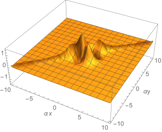
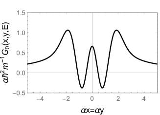
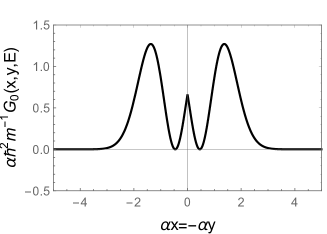
Figure 1: 3D plot of $\alpha\hbar^{2}m^{-1}G_{0}(x,y,E)$ using Eq. (19) with $\varepsilon=2.1$ for (a) $-5<\alpha x,\alpha y<5$ and (b) $-10<\alpha x,\alpha y<10$, and the section views along the line $x=y$ in (c) and the line $x=-y$ in (d), respectively.

For illustration, we plot $G_{0}(x,y,E)$ for $\varepsilon=2.1$ in Fig. 1. Note that the relations stated in Eq. (21) can be seen from the plots, where the graphs are clearly both mirror symmetric to the $x=y$ and the $x=-y$ lines. It is interesting to see that $G_{0}$ has some activities around the origin and has two long (but damping) tails along the $x=y$ line (in the positive $x,y$ and the negative $x,y$ directions) and remains highly suppressed in other region.

The energy eigenvalues and eigenvectors can be easily obtained from the above $G_{0}$. It is well known that the Gamma function $\Gamma(\frac{1}{2}-\varepsilon)$ has poles at

$$\frac{1}{2}-\varepsilon=-n\equiv\frac{1}{2}-\varepsilon_{n},\quad n=0,1,2,3,\dots,$$ (23)

giving the well known result:

$$E_{n}=\frac{\alpha^{2}\hbar^{2}}{m}\varepsilon_{n}=(n+\frac{1}{2})\hbar\omega,$$ (24)

and from

$$\lim_{\varepsilon\to\varepsilon_{n}}(\varepsilon_{n}-\varepsilon)\Gamma(\frac{1}{2}-\varepsilon)=\frac{(-1)^{n}}{\Gamma(n+1)},$$ (25)

we obtain

$$\lim_{E\to E_{n}}(E_{n}-E)G_{0}(x,y,;E) = \frac{\alpha}{2^{n}\sqrt{\pi}\,\Gamma(n+1)}e^{-\frac{\alpha^{2}(x^{2}+y^{2})}{2}}H_{n}\left(\alpha x\right)H_{n}\left(\alpha y\right),$$ (26)

which is just $u_{n}(x)u^{*}_{n}(y)$, where $u_{n}(x)$ is the usual time-independent wave function of simple harmonic oscillator

$$u_{n}(x)=\eta\left(\frac{\alpha}{2^{n}\sqrt{\pi}\,\Gamma(n+1)}\right)^{1/2}e^{-\frac{\alpha^{2}x^{2}}{2}}H_{n}\left(\alpha x\right),$$ (27)

with $\eta$ is a phase factor conventionally taken to be 1.

In summary the poles of $G_{0}$ are determined from the zeros of the Wronskian, $W(f_{<}(x),f_{>}(x))$. As noted for $\nu\neq n$ the Wronskian is not vanishing, while for $\nu=n$, $f_{<}(x)$ and $f_{>}(x)$ are linearly dependent as shown in Eq. (20). Therefore $\nu\equiv\varepsilon-1/2=n$ are the zeros of the Wronskian and hence the poles of the Green’s function.

A related observation at the wave function level was given in ref. Viana-Gomes . We can redo their argument using the technic similar to the above derivation and give further insight into the problem. We express the wave function $u_{\nu}(x)$ as

$$u_{\nu}(x) = Ne^{-\frac{\alpha^{2}(x^{2}+y^{2})}{2}}H_{\nu}\left(-\alpha\min(x,y)\right)H_{\nu}\left(\alpha\max(x,y)\right),$$ (28)

with $\nu=\varepsilon-1/2$, $N$ a normalization factor, and an arbitrary $y$ as long as $H_{\nu}(\pm\alpha y)$ is non-vanishing. By construction the wave function is guaranteed to be continuous at $x=y$ and is the solution of the Schrödinger equation (for $x\neq y$)

$$\left(-\frac{\hbar^{2}}{2m}\frac{\partial^{2}}{\partial x^{2}}+\frac{1}{2}m\omega^{2}x^{2}\right)u_{\nu}(x)=Eu_{\nu}(x),$$ (29)

satisfying the boundary conditions

$$\lim_{x\to\pm\infty}u_{\nu}(x)=0,$$ (30)

for any (real) value of $\varepsilon=\nu+1/2$. As pointed out in ref. Viana-Gomes , in contrary to the usual treatment in most text books, the satisfactions of these requirements do not necessarily lead to a viable wave function solution. A viable solution of the above Schrödinger equation (including $x=y$) requires the derivative of the wave function to be continuous as well Viana-Gomes . It can be easily seen that this requires, at the matching point ($x=y$), that we must have

$$0=\frac{1}{N}u^{\prime}_{\nu}(x)\Big{|}^{y^{+}}_{y^{-}}=W(f_{<}(y),f_{>}(y))=e^{-\alpha y^{2}}W\left(H_{\nu}(-\alpha y),H_{\nu}(\alpha y)\right)=\frac{2^{\varepsilon-1/2}\sqrt{\pi}\alpha}{\Gamma(\frac{1}{2}-\varepsilon)},$$ (31)

giving $\nu=\varepsilon-1/2=n$, and

$$u_{n}(x)=N^{\prime}e^{-\frac{\alpha^{2}x^{2}}{2}}H_{n}\left(\alpha x\right),$$ (32)

where $N^{\prime}\equiv(-1)^{n}N\exp(-\alpha^{2}y^{2}/2)H_{n}(\alpha y)$. Note that this happens only at $\nu=n$, where $H_{\nu}(-\alpha x)$ and $H_{\nu}(\alpha x)$ are linearly dependent [see Eq. (20)] and produce a vanishing Wronskian.

In fact, it is exactly the same place and the very same source where the Green’s function $G_{0}$ has poles in $E$ [see Eqs. (17) and (18)]. At a first sight it seems that this is just a coincident, as the Wronskian in $G_{0}$ is to assure the Green’s function to satisfy the matching condition or discontinuity condition, Eq. (8), while the Wronskian in $u_{\nu}$ is to govern the continuity of the wave function at $y$ and is required to be vanishing to give a viable wave function. To see the connection we rewrite $G_{0}(x,y;E)$ in Eq. (17), with the help of Eq. (28), as

$$G_{0}(x,y;E) = -\frac{2m}{\hbar^{2}}\frac{u_{\nu}(x)/N}{W\left(e^{-\alpha^{2}y^{2}/2}H_{\varepsilon-1/2}(-\alpha y),e^{-\alpha^{2}y^{2}/2}H_{\varepsilon-1/2}(\alpha y)\right)}.$$ (33)

and, consequently,

$$\Delta G^{\prime}_{0}\equiv\frac{\partial}{\partial x}G_{0}(x,y;E)\Big{|}^{x=y^{+}}_{x=y^{-}} = -\frac{2m}{\hbar^{2}N}\frac{u^{\prime}_{\nu}(x)\big{|}^{y^{+}}_{y^{-}}}{W\left(e^{-\alpha^{2}y^{2}/2}H_{\varepsilon-1/2}(-\alpha y),e^{-\alpha^{2}y^{2}/2}H_{\varepsilon-1/2}(\alpha y)\right)}.$$ (34)

The matching condition or discontinuity condition requires the derivative of $G_{0}$ to be discontinuous at $x=y$, i.e. $\Delta G^{\prime}_{0}=-2m/\hbar\neq 0$. However, as $\varepsilon$ approaching $n+1/2$, the derivative of the numerator of $G_{0}$ in Eq. (33) tends to be continuous at $x=y$ [see Eq. (31)], leading to a vanishing numerator in $\Delta G^{\prime}_{0}$ [see Eq. (34)]. The Wronskian in the denominator of $\Delta G^{\prime}_{0}$ keeps doing it’s job to assure $G^{\prime}_{0}$ to satisfy the discontinuity condition by balancing the Wronskian from the derivative of the numerator. Hence a continuous $u^{\prime}_{\nu}$ at $x=y$ corresponds to a vanishing Wronskian in the denominator in $G_{0}$. The Wronskians in the numerator and the denominator of $\frac{\partial}{\partial x}G_{0}(x,y;E)\big{|}^{x=y^{+}}_{x=y^{-}}$ as shown in the above equation are the very same Wronskian as required from the matching condition Eq. (8). In short, the poles of $G_{0}$ in $E$ is tied to the continuity of $u^{\prime}_{\nu}$ at $x=y$.

We see that the Wronskian plays some interesting and important roles in $G_{0}$ and $u_{\nu}$. Although it is possible to obtain $G_{0}(x,y;E)$ by performing the Fourier transform of $K_{0}(x,t;y,t_{0})$ using an integral of Bessel function Kleinert:2004ev , the interesting point we see in the above discussion will be obscured.

III Time-independent Green’s function of a quantum simple harmonic oscillator with a generic delta-function potential

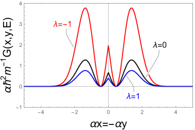
Figure 2: Section views of $\alpha\hbar^{2}m^{-1}G(x,y;E)$ with $V_{1}(x)=\frac{\alpha\hbar^{2}}{m}\lambda\delta(x)$ and $\varepsilon=2.1$ along the line $x=y$ in (a) and the line $x=-y$ in (b).

In this section, we follow the approach of ref. Cavalcanti to obtain the Green’s functions for SHO with an additional delta-function potential. Let $H_{0}$, $G_{0}$ and $H$, $G$ be the Hamiltonian and the Green’s function of the quantum systems of pure SHO and SHO with a delta-function potential $V_{1}(x)=\frac{\alpha\hbar^{2}}{m}\lambda\delta(x-a)$, respectively. Hence we have

$$(H_{0}-E)G_{0}(x,y;E)=\delta(x-y),\quad(H-E)G(x,y;E)=\delta(x-y),$$ (35)

where $H=H_{0}+V_{1}$. In the above, the second equation can be rewritten as

$$(H_{0}-E)G(x,y;E)=\delta(x-y)-V_{1}(x)G(x,y;E).$$ (36)

Multiplying $G_{0}(y,x)$ on both sides and integrating them with respective to $x$ from $-\infty$ to $\infty$, we obtain the following relation:

$$G(x,y;E) = G_{0}(x,y;E)-\frac{\alpha\hbar^{2}}{m}G_{0}(x,a;E)G(a,y;E),$$ (37)

which gives Cavalcanti

$$G(x,y;E)=G_{0}(x,y;E)-\frac{G_{0}(x,a;E)G_{0}(a,y;E)}{\frac{1}{\frac{\alpha\hbar^{2}}{m}\lambda}+G_{0}(a,a;E)}.$$ (38)

Using Eq. (19), the Green’s function of the quantum system of SHO with a delta-function potential $V_{1}(x)=\frac{\alpha\hbar^{2}}{m}\lambda\delta(x-a)$ can be written explicitly as

$$G(x,y;E) = \frac{m\Gamma(\frac{1}{2}-\varepsilon)}{{{2}^{\varepsilon-1/2}}\sqrt{\pi}\alpha{{\hbar}^{2}}}{{e}^{-\frac{{{\alpha}^{2}}({{x}^{2}}+{{y}^{2}})}{2}}}{{H}_{\varepsilon-1/2}}\left(-\alpha\min(x,y)\right){{H}_{\varepsilon-1/2}}\left(\alpha\max(x,y)\right)$$ (39)

$$-\frac{{{\left(\frac{m\Gamma(\frac{1}{2}-\varepsilon)}{{{2}^{\varepsilon-1/2}}\sqrt{\pi}\alpha{{\hbar}^{2}}}\right)}^{2}}{{e}^{-\frac{{{\alpha}^{2}}({{x}^{2}}+{{y}^{2}})}{2}}}}{\frac{m}{\lambda\alpha{{\hbar}^{2}}}+\frac{m\Gamma(\frac{1}{2}-\varepsilon)}{{{2}^{\varepsilon-1/2}}\sqrt{\pi}\alpha{{\hbar}^{2}}}H_{\varepsilon-1/2}(-\alpha a)H_{\varepsilon-1/2}(\alpha a)}$$

$$\quad\times{{H}_{\varepsilon-1/2}}\left(-\alpha\min(x,a)\right){{H}_{\varepsilon-1/2}}\left(\alpha\max(x,a)\right)$$

$$\quad\times{{H}_{\varepsilon-1/2}}\left(-\alpha\min(a,y)\right){{H}_{\varepsilon-1/2}}\left(\alpha\max(a,y)\right).$$

For illustration we plot the section views of $G(x,y;E)$ in the case of $a=0$ with $\varepsilon=2.1$ along the line $x=y$ in Fig. 2(a) and the line $x=-y$ in Fig. 2(b), respectively. We can see clearly the discontinuity of first derivative of $G(x,y;E)$ at origin for $\lambda=\mp 1$ in the plots.

It is well known that by analysing the pole of $G(x,y;E)$ in $E$ one can obtain the energy levels $E_{n}$. From Eq. (39), by taking $x=y=a\neq 0$, we have

$$G(a,a;E)=\frac{me^{-\alpha^{2}a^{2}}H_{\varepsilon-1/2}(-\alpha a)H_{\varepsilon-1/2}(\alpha a)}{\alpha\hbar^{2}\bigg{(}\frac{\sqrt{\pi}2^{\varepsilon-1/2}}{\Gamma(1/2-\varepsilon)}+\lambda e^{-\alpha^{2}a^{2}}H_{\varepsilon-1/2}(-\alpha a)H_{\varepsilon-1/2}(\alpha a)\bigg{)}},$$ (40)

we can obtain the following transcendental equation from the poles of the above function:

$$\frac{2^{\varepsilon+1/2}\sqrt{\pi}}{\Gamma(\frac{1}{2}-\varepsilon)}+2\lambda e^{-\alpha^{2}a^{2}}H_{\varepsilon-1/2}(-\alpha a)H_{\varepsilon-1/2}(\alpha a)=0.$$ (41)

It can be easily seen that in the $\lambda=0$ limit, we return to the familiar energy level of the SHO case [see Eq. (23)].

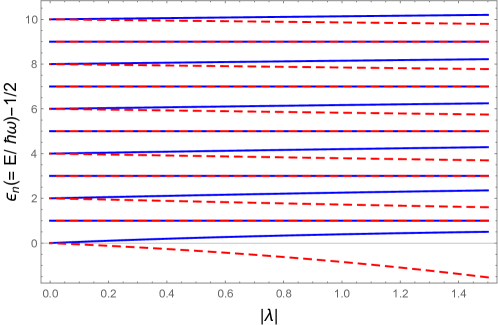
Figure 3: The plot of energy eigenvalue $\varepsilon_{n}-1/2$ versus the coupling strength $\lambda$ is shown. The solid and the dashed line correspond with $\lambda>0$ and $\lambda<0$, respectively.

We can compare our result with the one in ref. Viana-Gomes by taking the $a\to 0$ limit.  Fig. 3 shows the plot of the first eleven energy eigenvalues $\varepsilon_{n}-1/2$ $(n=0,1,\cdots,10)$ versus the coupling strength $\lambda$ in the region $-1.5\leq\lambda\leq 1.5$. For $\lambda=0$ or $n$ is odd, the energy eigenvalues go back to those in the pure quantum SHO system. This can be easily understood: since in the presence of the $\delta(x)$ potential, the full potential in the Schrödinger equation is still parity even giving parity even and odd solutions, the energy levels of the parity odd states are unaffected by the $\delta(x)$ potential as the odd wave function is vanishing at the origin. For $n$ is even, we see that the energy eigenvalue increases with increasing $\lambda$, but it never crosses over the adjacent eigenvalues of odd energy levels. To be specific, we show the numerical values of the first six even parity eigenvalues $\varepsilon_{n}-1/2$ for $\lambda=0,\mp 0.5$ and $\mp 1$ in Table 1. Our results agree well with those in ref. Viana-Gomes .

$\varepsilon_{n}-1/2$	$n=0$	$n=2$	$n=4$	$n=6$	$n=8$	$n=10$
$\lambda=0$	0	2	4	6	8	10
$\lambda=-0.5$	-0.344434	1.85734	3.89395	5.91181	7.92289	9.93062
$\lambda=0.5$	0.233518	2.13541	4.10367	6.08703	8.07642	10.0689
$\lambda=-1$	-0.842419	1.72077	3.79123	5.82578	7.84733	9.86242
$\lambda=1$	0.392744	2.25464	4.2002	6.16991	8.15009	10.1359

Table 1: The first six even parity eigenvalues $\varepsilon_{n}-1/2$ for $\lambda=0,\mp 0.5,\mp 1$.

IV Solutions of Schrödinger equation of a simple harmonic oscillator system with a generic delta-function potential

In this section, the similar technics previously used to solve the Green’s function can also be applied to solving the wave function directly from the Schrödinger equation. We first write down the Schrödinger equation for the quantum system of SHO with a generic delta-function potential:

$$\left(-\frac{\hbar^{2}}{2m}\frac{\partial^{2}}{\partial x^{2}}+V(x)\right)v(x;a)=Ev(x;a),$$ (42)

where

$$V(x)=\frac{1}{2}m\omega^{2}x^{2}+\frac{\alpha\hbar^{2}}{m}\lambda\delta(x-a)=V_{0}(x)+V_{1}(x).$$ (43)

The wave function needs to satisfy the boundary conditions:

$$\lim_{x\to\pm\infty}v(x;a)=0,$$ (44)

and the matching conditions around $x=a$:

$$v(x=a^{+};a)=v(x=a^{-};a),$$ (45)

$$\frac{\partial}{\partial x}v(x=a^{+};a)-\frac{\partial}{\partial x}v(x=a^{-};a)=2\alpha\lambda v(a;a).$$ (46)

Using the same technics in Sec. II, we assume that the wave function is of the form:

$$v_{\nu}(x;a) = Ne^{-\frac{\alpha^{2}(x^{2}+a^{2})}{2}}H_{\nu}\left(-\alpha\min(x,a)\right)H_{\nu}\left(\alpha\max(x,a)\right),$$ (47)

where $N$ is the the normalization constant and $\nu=\varepsilon-1/2$.

$\varepsilon_{n}-1/2$	$n=0$	$n=1$	$n=2$	$n=3$	$n=4$	$n=5$
$\lambda=0$	0	1	2	3	4	5
$\lambda=-0.5$	-0.288982	0.895074	1.97192	2.88647	3.99943	4.90350
$\lambda=0.5$	0.16908	1.10823	2.02645	3.11238	4.00057	5.09438
$\lambda=-1$	-0.750901	0.809830	1.954355	2.78069	3.99885	4.80935
$\lambda=1$	0.267782	1.20385	2.05035	3.21619	4.00114	5.18277

Table 2: The first six exact and perturbed energy eigenvalues $\varepsilon_{n}-1/2$ for $\alpha a=0.5$ with $\lambda=0,\mp 0.5,\mp 1$ are shown.

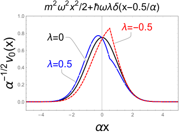
(a)  $n=0$

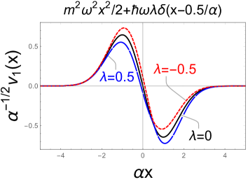
(b)  $n=1$

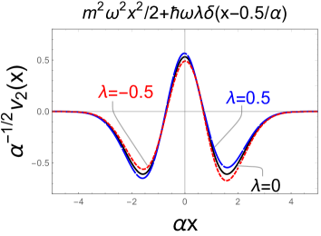
(c)  $n=2$

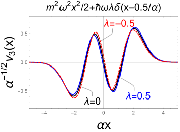
(d)  $n=3$

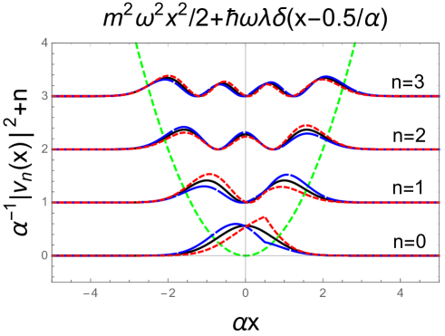
Figure 4: (a)-(d): The plots of wave functions $\alpha^{-1/2}v_{n}(x)$ corresponding to the first four energy levels $n=0,1,2,3$ with $\lambda=0,\pm 0.5$, respectively are shown. (e): The absolute square values of wave functions, $\alpha^{-1}|v_{n}(x)|^{2}$, corresponding to the first four energy levels $n=0,1,2,3$ with $\lambda=0.5$ (long-dashed), $\lambda=-0.5$ (dashed), and $\lambda=0$ (solid), respectively are shown.

With the help of Eq. (18) we obtain the following transcendental equation from Eq. (46):

$$\frac{2^{\varepsilon+1/2}\sqrt{\pi}}{\Gamma(\frac{1}{2}-\varepsilon)}+2\lambda e^{-\alpha^{2}a^{2}}H_{\varepsilon-1/2}(-\alpha a)H_{\varepsilon-1/2}(\alpha a)=0,$$ (48)

which is exactly the same as in Eq. (41). This equation gives us the relation between the coupling strength $\lambda$ and the energy (in $\hbar\omega$ unit) eigenvalue $\varepsilon=\varepsilon_{n}$, and for a given $\lambda$, we can get the eigenvalue by numerically solving this equation.

In Table. 2, we show the first six energy eigenvalues $\varepsilon_{n}-1/2$ for $\alpha a=0.5$ and $\lambda=0,\pm 0.5,\pm 1$, respectively. We see that the eigenvalues increase with increasing the coupling strength $\lambda$ and never cross over the adjacent energy levels.

In Fig. 4(a)-(d), we plot the the wave functions $v_{n}(x)$ corresponding to the first four energy levels $n=0,1,2,3$ with $\lambda=0,\pm 0.5$, respectively. It is apparent to see the discontinuity of the first derivative of $v_{0}(x)$ with $\lambda=\pm 0.5$ at the $\alpha x=0.5$ in Fig. 4(a), but not so apparent in Fig. 4(b-d). We also see that the discontinuity disappears as the coupling strength $\lambda$ goes to 0. On the other hand, $\lambda<0$ ($\lambda>0$) corresponds to attractive (repulsive) force so that we have a larger (smaller) amplitude of wave function at $\alpha x=0.5$ with $\lambda=-0.5$ (0.5) than the original one in Fig. 4(a). In Fig. 4(e), we plot the absolute square values of wave functions, $|v_{n}(x)|^{2}$, corresponding to the first four energy levels $n=0,1,2,3$ with $\lambda=0.5$ (long-dashed), $\lambda=-0.5$ (dashed), and $\lambda=0$ (solid), respectively. We see that there is more probability to appear on the right-hand side of the line $x=0$ than the left-hand for even $n$ and it is reversed for odd $n$ for $\lambda=-0.5$. On the contrary, there is fewer probability to appear on the right-hand side of the line $x=0$ than the left-hand for even $n$ and it is reversed for odd $n$ for $\lambda=0.5$.

V Solutions of Schrödinger equation of a simple harmonic oscillator system with two generic delta-function potentials

In this section, we generalize the technics to solving the quanatum system of SHO with two generic delta-function potentials. The corresponding Schrödinger equation is

$$\left(-\frac{\hbar^{2}}{2m}\frac{\partial^{2}}{\partial x^{2}}+V(x)\right)v((x;y_{1},y_{2})=Ev(x;y_{1},y_{2}),$$ (49)

where

$$V(x)=\frac{1}{2}m\omega^{2}x^{2}+\frac{\alpha\hbar^{2}}{m}\lambda_{1}\delta(x-y_{1})+\frac{\alpha\hbar^{2}}{m}\lambda_{2}\delta(x-y_{2}).$$ (50)

Without loss of generality, we have assumed that $y_{1}<y_{2}$ in the above. Similarly, after changing the variable as in Eq. (4), we have

$$\left(\frac{\partial^{2}}{\partial x^{2}}-\alpha^{4}x^{2}+2\alpha^{2}\varepsilon\right)v(x;y_{1},y_{2})=2\alpha\lambda_{1}\delta(x-y_{1})v(x;y_{1})+2\alpha\lambda_{2}\delta(x-y_{2})v(x;y_{2}).$$ (51)

The wave function needs to satisfy the boundary conditions:

$$\lim_{x\to\pm\infty}v(x;y_{1},y_{2})=0,$$ (52)

and the matching conditions around $x=y_{1}$ and $x=y_{2}$:

$$v(x=y_{1}^{+};y_{1},y_{2})=v(x=y_{1}^{-};y_{1},y_{2}),\quad v(x=y_{2}^{+};y_{1},y_{2})=v(x=y_{2}^{-};y_{1},y_{2}),$$ (53)

$$\frac{\partial}{\partial x}v(x=y_{1}^{+};y_{1},y_{2})-\frac{\partial}{\partial x}v(x=y_{1}^{-};y_{1},y_{2})=2\alpha\lambda v(y_{1};y_{1},y_{2}),$$

$$\frac{\partial}{\partial x}v(x=y_{2}^{+};y_{1},y_{2})-\frac{\partial}{\partial x}v(x=y_{2}^{-};y_{1},y_{2})=2\alpha\lambda v(y_{2};y_{1},y_{2}).$$ (54)

The wave function is assumed to have the following form:

$$v(x;y_{1},y_{2}) = Nf_{<}\left(\min(x,y_{1})\right)f_{\parallel}(\min(\max(x,y_{1}),y_{2}))f_{>}\left(\max(x,y_{2})\right).$$ (55)

where $N$ is the normalization constant and

$$f_{<}(x) = e^{-\frac{\alpha^{2}x^{2}}{2}}H_{\nu}(-\alpha x),$$

$$f_{\parallel}(x) = e^{-\frac{\alpha^{2}x^{2}}{2}}[H_{\nu}(-\alpha x)+\beta H_{\nu}(\alpha x)],$$

$$f_{>}(x) = e^{-\frac{\alpha^{2}x^{2}}{2}}H_{\nu}(\alpha x).$$ (56)

In the above, $\nu=\varepsilon-1/2$ and the coefficient $\beta$ are undetermined. The discontinuities of the first derivatives of the wave function $v(x)$ at $x=y_{1}$ and $x=y_{2}$ [see Eq. (54)] give us a set of two simultaneous equations:

$$W\left(f_{<}(y_{1}),f_{\parallel}(y_{1})\right) = 2\alpha\lambda e^{-\alpha^{2}y_{1}^{2}}H_{\varepsilon-1/2}(-\alpha y_{1})H_{\varepsilon-1/2}(\alpha y_{1}),$$

$$W\left(f_{\parallel}(y_{2}),f_{>}(y_{2})\right) = 2\alpha\lambda e^{-\alpha^{2}y_{2}^{2}}H_{\varepsilon-1/2}(-\alpha y_{2})H_{\varepsilon-1/2}(\alpha y_{2}).$$ (57)

For a given coupling strength $\lambda$, we can numerically solve the eigenvalue $\varepsilon=\varepsilon_{n}$ and the coefficient $\beta$ from the above two simultaneous equations. For simplicity, we consider the case: $\lambda_{1}=\lambda_{2}\equiv\lambda$ and $y_{1}=-y_{2}$ so that the potential is symmetric, i.e. $V(-x)=V(x)$, and hence the wave function $v_{n}(x)$ must be even or odd. From Eq. (55) and Eq. (56), we know that $\beta=1$ for even function $v_{n}(x)$ and $\beta=-1$ for the odd function $v_{n}(x)$. We note that in passing the above transcendental equations are much simpler than those shown in ref. FB .

$\varepsilon_{n}-1/2$	$n=0$	$n=1$	$n=2$	$n=3$	$n=4$	$n=5$
$\lambda=0$	0	1	2	3	4	5
$\lambda=-0.5$	-0.49476	0.711225	1.9511	2.75301	3.99888	4.81243
$\lambda=0.5$	0.389598	1.17256	2.06173	3.2031	4.00117	5.18881
$\lambda=-1$	-1.11286	0.230993	1.91252	2.50163	3.9978	4.64815
$\lambda=1$	0.689733	1.28047	2.13806	3.35457	4.00238	5.35735

Table 3: The first six energy eigenvalues $\varepsilon_{n}-1/2$ for $\alpha y_{1}=0.5,\alpha y_{2}=-0.5$ and $\lambda_{1}=\lambda_{2}\equiv\lambda=0,\mp 0.5,\mp 1$ are shown.

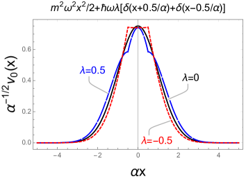
(a)  $n=0$ 

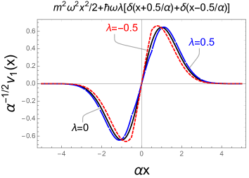
(b)  $n=1$ 

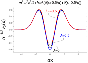
(c)  $n=2$ 

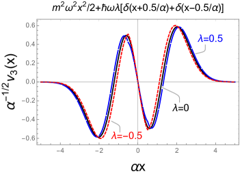
(d)  $n=3$ 

Figure 5: (a)-(d): The plots of wave functions $\alpha^{-1/2}v_{n}(x)$ corresponding to the first four energy level $n=0,1,2,3$ with $\lambda=0,\pm 0.5$, respectively are shown. (e): The absolute square values of wave functions, $\alpha^{-1}|v_{n}(x)|^{2}$, corresponding to the first four energy levels $n=0,1,2,3$ with $\lambda=0.5$ (long-dashed), $\lambda=-0.5$ (dashed), and $\lambda=0$ (solid), respectively are shown.

In Table. 3, we show the first six energy eigenvalues $\varepsilon_{n}-1/2$ for $\alpha y_{1}=-0.5,\ \alpha y_{2}=0.5$ and $\lambda=0,\pm 0.5,\pm 1$, respectively. We also see that the eigenvalues increase with increasing the coupling strength $\lambda$ and never cross over the adjacent energy level as in the previously case. In Fig. 5(a)-(d), we plot the the wave functions $v_{n}(x)$ corresponding to the first four energy levels $n=0,1,2,3$ with $\lambda=0,\pm 0.5$, respectively. Since the Hamiltonian is parity invariant, the wave function $v_{n}(x)$ is either even or odd. It is apparent to see the discontinuity of the first derivatives of the wave function $v_{n}(x)$ at the $\alpha x=\pm 0.5$ with $\lambda=\pm 0.5$ in Fig. 5(a), but not so apparent in Fig. 5(b-d). We also see that the discontinuity disappears as the coupling strength $\lambda$ goes to 0. In Fig. 5(e), we plot the absolute square values of wave functions, $|v_{n}(x)|^{2}$, corresponding to the first four energy levels $n=0,1,2,3$ with $\lambda=0.5$ (long-dashed), $\lambda=-0.5$ (dashed), and $\lambda=0$ (solid), respectively. Since $\lambda<0$ ($\lambda>0$) corresponds to the attractive (repulsive) force, in general, we have a larger (smaller) square amplitude of wave function at $\alpha x=\pm 0.5$ than the $\lambda=0$ case.

VI Conclusions

We study the one-dimensional problem on the quantum system of SHO without/with one (or two) generic delta-function potential(s). For the pure quantum SHO system, we derive a complete analytical form for the corresponding time-independent Green’s function. It is natural and straightforward to obtain eigenvalues and eigenfunctions from the Green’s function. The energy eigenvalues can be obtained from the poles of the Green’s function and using the residue theorem, we can obtain the familiar SHO wave functions. We see that the Wronskian plays the interesting and important roles in $G_{0}$ and the wave function $u_{\nu}$ [see Eq. (28)]. Although it is possible to obtain $G_{0}(x,y;E)$ by performing the Fourier transform of $K_{0}(x,t;y,t_{0})$ using an integral of Bessel function Kleinert:2004ev , the above interesting point will be obscured. For the quantum SHO system with a generic delta-function potential, we follow the approach of ref. Cavalcanti to obtain the time-independent Green’s function from the SHO Green’s function obtained previously. The eigenvalues can be obtained from the poles of the Green’s function. Our results agree with Viana-Gomes , but our method can also be applied to a delta-function potential at an arbitrary site. Nevertheless, the simplest way to find the wave functions is to solve the Schrödinger equation directly. In fact, the same technics of solving the Green’s function $G_{0}$ can be used to solve the eigenvalue problem of the simple harmonic oscillator with an generic delta-function potential at an arbitrary site. The technics can be easily generalized to solve the quantum system of SHO with two generic delta-function potentials. For illustration, we solve the case of symmetric potential and obtain energy eigenvalues and eigenstates for the first few states.

References

- (1) S. Gasiorowicz, Quantum Physics, 3rd Ed., John Wiley Son, 2003.
- (2) S. C. Bloch, Introduction to Classic and Quantum Harmonic Oscillators, Wiley-Blackwell, New York, 1997.
- (3) M. Moshinsky and Yuri F. Smirnov, The Harmonic Oscillator in Modern Physics, 2nd Ed., Harwood- Academic Publishers, Amsterdam, 1996.
- (4) N. R. Kestner and O. Sinanoglu, “Study of electron correlation in Helium-like system using an exactly soluble model”, Phy. Rev. 128, 2687 (2011).
- (5) S. Franz, Admanced Quantum Mechanics, 4th Ed., Springer 2008.
- (6) R. B. Laughlin, “Quantized Hall conductivity in two-dimensions,” Phys. Rev. B 23, 5632 (1981).
- (7) C. Yannouleas and U. Landman, “Spontaneous symmetry breaking in single and molecular quantum dots,” Phys. Rev. Lett. 82, 5325 (1999). Erratum: [Phys. Rev. Lett. 85, 2220 (2000)], [cond-mat/9905383].
- (8) N. N. Lebedev, Special Functions & Their Applications, Dover 1972.
- (9) David J. Griffiths, Introduction to Quantum Mechanics, 2nd Ed., Person, 2005.
- (10) https://en.wikiquote.org/wiki/Sidney_Coleman.
- (11) Douglas R M Pimentel and Antonio S de Castro, “A Laplace transform approach to the quantum harmonic oscillator,” Eur. J. Phys. 34, 199 (2013).
- (12) P. H. F. Nogueira and A. S. de Castro, “Revisiting the quantum harmonic oscillator via unilateral Fourier transforms,” Eur. J. Phys. 37, 015402 (2016).
- (13) J. Viana-Gomes, N. M. R. Peres, “Solution of the quantum harmonic oscillator plus a delta-function potential at the origin: The oddness of its even-parity solutions”, Eur. J. Phys. 32, 1377 (2011), arXiv:1109.3077.
- (14) S H Patil, “Harmonic oscillator with a -function potential,” Eur. J. Phys. 27, 899 (2006).
- (15) E. N. Economou, Green’s Functions in Quantum Physics, 3rd Ed., Springer, 2006.
- (16) J. J. Sakurai and J. Napolitano, “Modern quantum physics,” Boston, USA, Addison-Wesley (2011); R. P. Feynman and A. R. Hibbs, “Quantum Mechanics and Path Integrals,” New York, McGraw-Hil (1965) .
- (17) Yu-Tsai Liu, “Time-independent Green’s function of a quantum simple harmonic oscillator and solutions with additional generic delta function potentials,” Master Thesis (in Chinese), Chung Yuan Christian University, Taiwan, R.O.C., 2017.
- (18) J. D. Jackson, Classical Electrodynamics, 3rd Ed., Wiley 1998, §3.11.
- (19) H. Kleinert, “Path Integrals in Quantum Mechanics, Statistics, Polymer Physics, and Financial Markets,” World Scientific, Singapore, 2004, §9.2.
- (20) R. M. Cavalcanti, “Exact Green’s functions for delta function potentials and renormalization in quantum mechanics,” Rev. Bras. Ens. Fis. 21, 336 (1999) [quant-ph/9801033].
- (21) N. Ferkous and T. Boudjedaa, “Bound States Energies of a Harmonic Oscillator Perturbed by Point Interactions,” Commun. Theor. Phys. 67 241 (2017).