Learning-based Caching in Cloud-Aided Wireless Networks

Syed Tamoor-ul-Hassan1, Sumudu Samarakoon1, Mehdi Bennis1, Matti Latva-aho1, Choong-Seong Hong2
1Center for Wireless Communications, University of Oulu, Finland,
email: {tsyed, bennis, sumudu, matti.latva-aho}@ee.oulu.fi
2Department of Computer Engineering, Kyung Hee University, South Korea, email: cshong@khu.ac.kr
Abstract

This paper studies content caching in cloud-aided wireless networks where small cell base stations with limited storage are connected to the cloud via limited capacity fronthaul links. By formulating a utility (inverse of service delay) maximization problem, we propose a cache update algorithm based on spatio-temporal traffic demands. To account for the large number of contents, we propose a content clustering algorithm to group similar contents. Subsequently, with the aid of regret learning at small cell base stations and the cloud, each base station caches contents based on the learned content popularity subject to its storage constraints. The performance of the proposed caching algorithm is evaluated for sparse and dense environments while investigating the tradeoff between global and local class popularity. Simulation results show 15% and 40% gains in the proposed method compared to various baselines.

I Introduction

Edge caching represents a viable solution to overcome challenges associated with network densification by intelligently caching contents at the network edge [1]. Besides reducing latency, edge caching also offloads the backhaul traffic load [2]. Existing literature investigates the potential benefits of caching in terms of backhaul offloading gains and latency [3, 4, 5]. While these works show improved network performance through caching, they neglect the intrinsic user behavior by considering a fixed caching policy. Due to the spatio-temporal requests, small cell base stations (SBSs) often need to update their cache following their local request distribution to minimize latency [6]. In such scenarios, optimal content placement becomes a challenging and non-trivial problem. To serve user requests, the works in [7, 8, 9] proposed dynamic caching algorithms based on fixed content popularity. However, these works assume a small content library with fixed content popularities. With the growing library size, determining popularity and content caching becomes computationally expensive. Recently, grouping contents based on their popularity was proposed in [10]. However, how to group contents and cache accordingly based on time-varying popularity was not studied.
The main contribution of this paper is to revisit the fundamental problem of content caching under spatio-temporal traffic demands in cloud-aided wireless networks and explore the tradeoffs between global and local content popularity. By considering a random deployment of SBSs and users, the objective is to determine what contents need to be cached locally by every SBS so as to maximize the cache hit rate. Based on the instantaneous content requests, each SBS locally learns the time-varying content popularity with the aid of regret learning [11]. Simultaneously, the cloud learns the global content popularity. By randomizing its caching strategy, each SBS optimizes the caching policy in a decentralized manner and updates its cache.

II System Model and Problem Formulation

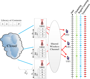
Consider the downlink transmission of a small cell network comprised of randomly deployed SBSs, $\mathcal{S}=\{1,...,S\}$ with intensity $\lambda_{\mathrm{SBS}}$. Let Yssubscript๐‘Œ๐‘ Y_{s} represent the location of the s๐‘ s-th SBS. Each SBS serves a set of user equipment(s) (UEs), $\mathcal{U}=\{1,...,U\}$, deployed randomly with intensity $\lambda_{\mathrm{UE}}$. The location of the $u$-th UE is denoted by $Z_{u}$. Each SBS serves UEsโ€™ requests over a common pool of spectrum with bandwidth $\omega$. Accordingly, the instantaneous data rate of UE $u$ served by SBS s๐‘ s is:

Rsโ€‹uโ€‹(t)=ฯ‰โ€‹log2โ€‹(1+psโ€‹โˆฅฮจsโ€‹uโ€‹(t)โˆฅ2ฯƒ2+โˆ‘sโ€ฒโˆˆ๐’ฎโˆ–spsโ€ฒโ€‹โˆฅฮจsโ€ฒโ€‹uโ€‹(t)โˆฅ2),subscript๐‘…๐‘ ๐‘ข๐‘ก๐œ”subscriptlog21subscript๐‘๐‘ superscriptdelimited-โˆฅโˆฅsubscriptฮจ๐‘ ๐‘ข๐‘ก2superscript๐œŽ2subscriptsuperscript๐‘ โ€ฒ๐’ฎ๐‘ subscript๐‘superscript๐‘ โ€ฒsuperscriptdelimited-โˆฅโˆฅsubscriptฮจsuperscript๐‘ โ€ฒ๐‘ข๐‘ก2R_{su}(t)=\omega\mathrm{log}_{2}\left(1+\frac{p_{s}\lVert\Psi_{su}(t)\rVert^{2}}{\sigma^{2}+\sum_{s^{\prime}\in\mathcal{S}\setminus s}p_{s^{\prime}}\lVert\Psi_{s^{\prime}u}(t)\rVert^{2}}\right),\vspace{-0.3cm} (1)

where $\sigma^{2}$ represents the variance of noise, pssubscript๐‘๐‘ p_{s} denotes the transmit power of SBS s๐‘ s and ฮจsโ€‹uโ€‹(t)subscriptฮจ๐‘ ๐‘ข๐‘ก\Psi_{su}(t) denotes the channel gain between UE $u$ and SBS s๐‘ s.
Each SBS is equipped with a cache of size $d$ where it stores contents from a content library $\mathcal{F}=\{1,...,F\}$ as shown in Fig. 1. Let $1/\mu$ be the size of all contents. In addition, let ๐šตโ€‹(t)=[๐šตsโ€‹(t)]sโˆˆ๐’ฎ๐šต๐‘กsubscriptdelimited-[]subscript๐šต๐‘ ๐‘ก๐‘ ๐’ฎ\boldsymbol{\Xi}(t)=[\boldsymbol{\Xi}_{s}(t)]_{s\in\mathcal{S}} represent the vector of SBSs cache at time $t$ where ๐šตsโ€‹(t)โІโ„ฑsubscript๐šต๐‘ ๐‘กโ„ฑ\boldsymbol{\Xi}_{s}(t)\subseteq\mathcal{F} represents the contents cached by SBS sโˆˆ๐’ฎ๐‘ ๐’ฎs\in\mathcal{S} at time $t$ such that |๐šตsโ€‹(t)|โ‰คdsubscript๐šต๐‘ ๐‘ก๐‘‘|\boldsymbol{\Xi}_{s}(t)|\leq d. We assume that SBSs partition the content library into popularity classes such that each content in a class is equally popular i.e., multi-class model [10]. Let the set of contents be partitioned into popularity classes $\mathcal{K}=\{1,2,...,K\}$, where $\mathcal{F}_{k}=\{1,...,F_{k}\}$ such that $\mathcal{F}_{k}\subset\mathcal{F}$, $\mathcal{F}_{k}\cap\mathcal{F}_{k^{\prime}}=\emptyset$, kโ‰ kโ€ฒ๐‘˜superscript๐‘˜โ€ฒk\neq k^{\prime}. Due to the constrained cache size and lack of coordination among SBSs, each SBS is connected to the cloud via a fixed capacity fronthaul link $C_{f}$ to obtain the global content popularity and update its cache accordingly.
Each UE requests contents from the library following the dynamic popularity model i.e., spatio-temporal model[12]. Let the content demanded by the $u$-th UE at time $t$ is denoted by $q_{u}(t)$ such that $q_{u}(t)\in\{0,1,2,...,F\}$ where $q_{u}(t)=0$ denotes no request by user $u$ at time $t$. For simplicity, we assume that each UE requests one content at a time. Let the content demand vector at SBS s๐‘ s be ๐‘ซsโ€‹(t)=[Dsโ€‹fโ€‹(t)]fโˆˆโ„ฑsubscript๐‘ซ๐‘ ๐‘กsubscriptdelimited-[]subscript๐ท๐‘ ๐‘“๐‘ก๐‘“โ„ฑ\boldsymbol{D}_{s}(t)=[D_{sf}(t)]_{f\in\mathcal{F}} such that Dsโ€‹fโ€‹(t)=โˆ‘uโˆˆ๐’ฉs๐Ÿ™quโ€‹(t)=fsubscript๐ท๐‘ ๐‘“๐‘กsubscript๐‘ขsubscript๐’ฉ๐‘ subscript1subscript๐‘ž๐‘ข๐‘ก๐‘“D_{sf}(t)=\sum_{u\in\mathcal{N}_{s}}\mathbb{1}_{q_{u}(t)=f} where $\mathbb{1}_{x}$ is the indicator function and ๐’ฉssubscript๐’ฉ๐‘ \mathcal{N}_{s} denotes the users in the coverage of SBS s๐‘ s.
The instantaneous reward of a SBS depends on the instantaneous cache hits and service rate. Absence of a requested content from a SBS incurs a cache miss. If the content is cached by multiple SBSs in UEโ€™s coverage, the user associates to the nearest SBS caching the requested content. In this regard, the reward of SBS s๐‘ s for serving UE $u$ is given by:

gsโ€‹quโ€‹(t,๐šตsโ€‹(t))=๐Ÿ™{quโ€‹(t)โˆˆ๐šตsโ€‹(t)}โ€‹Rsโ€‹uโ€‹(t).subscript๐‘”๐‘ subscript๐‘ž๐‘ข๐‘กsubscript๐šต๐‘ ๐‘กsubscript1subscript๐‘ž๐‘ข๐‘กsubscript๐šต๐‘ ๐‘กsubscript๐‘…๐‘ ๐‘ข๐‘กg_{sq_{u}}(t,\boldsymbol{\Xi}_{s}(t))=\mathbb{1}_{\{q_{u}(t)\in\boldsymbol{\Xi}_{s}(t)\}}R_{su}(t). (2)

II-A Utility Maximization Problem

The objective of SBSs is to determine a caching policy that maximizes their reward while ensuring UEs QoS. From (2), it can be observed that the reward of a SBS depends on the achievable rate and caching policy, i.e., SBS is rewarded if and only if it caches the requested content. For simplicity, fronthaul links are assumed to be used only for cache update and service rate is considered to be zero if the SBS has not cached the content. One of the challenges associated with cache update is when the number of most popular contents is larger than the cache size. In this case, SBSs must update their caching decisions carefully as caching less popular contents may decrease the SBSโ€™s reward.

Refer to caption
Figure 1: System Model

For a few UE requests, content popularity at SBSs may not be determined accurately, resulting in poor caching policy yielding lower reward. Hence, it is important that enough statistics are available to better learn the content popularity. To overcome this issue, the cloud estimates the global content popularity gathered from all SBSs. However, acquiring global demand and cache update incurs additional cost given by:

ฮตs=1โˆ’ฯ„sT2subscript๐œ€๐‘ 1subscript๐œ๐‘ subscript๐‘‡2\varepsilon_{s}=1-\frac{\tau_{s}}{T_{2}}\vspace{-0.25cm} (3)

where ฯ„s<T2subscript๐œ๐‘ subscript๐‘‡2\tau_{s}<T_{2} is the time required for cache update and $T_{2}$ represents the time during which the usersโ€™ requests are observed. Assume Cssubscript๐ถ๐‘ C_{s} is the fronthaul capacity for SBS s๐‘ s, the time required to update the cache of SBS s๐‘ s is:

ฯ„s=lpโ€‹Nฮผโ€‹Cs,subscript๐œ๐‘ subscript๐‘™๐‘๐‘๐œ‡subscript๐ถ๐‘ \tau_{s}=l_{p}\frac{N}{\mu C_{s}},\vspace{-0.2cm} (4)

where $l_{p}>0$ is a constant and $N$ represents the number of new contents. Let ฮžssubscriptฮž๐‘ \Xi_{s} be the vector of caching policies at SBS s over time $t=\{0,1,2,...\}$, i.e. ฮžs=[ฮžโ€‹(0),ฮžโ€‹(1),ฮžโ€‹(2),โ€ฆ]subscriptฮž๐‘ ฮž0ฮž1ฮž2โ€ฆ\Xi_{s}=[\Xi(0),\Xi(1),\Xi(2),...] and gยฏsโ€‹uโ€‹(๐šตs)=limtโ†’โˆžโ€‹1tโ€‹โˆ‘ฯ„=0tโˆ’1gsโ€‹quโ€‹(ฯ„,๐šตsโ€‹(ฯ„))subscriptยฏ๐‘”๐‘ ๐‘ขsubscript๐šต๐‘ subscriptlimโ†’๐‘ก1๐‘กsuperscriptsubscript๐œ0๐‘ก1subscript๐‘”๐‘ subscript๐‘ž๐‘ข๐œsubscript๐šต๐‘ ๐œ\bar{g}_{su}(\boldsymbol{\Xi}_{s})=\mathrm{lim}_{t\to\infty}\frac{1}{t}\sum_{\tau=0}^{t-1}g_{sq_{u}}(\tau,\boldsymbol{\Xi}_{s}(\tau)) be the limiting time-average reward at SBS s๐‘ s.Then, for each SBS sโˆˆ๐’ฎ๐‘ ๐’ฎs\in\mathcal{S}, the average per-SBS utility is the aggregate utility of the associated UEs i.e.,

ฮฅsโ€‹(๐šตs)=ฮตsโ€‹โˆ‘โˆ€uโˆˆ๐’ฉsฮฅsโ€‹uโ€‹(gยฏsโ€‹uโ€‹(๐šตs)),subscriptฮฅ๐‘ subscript๐šต๐‘ subscript๐œ€๐‘ subscriptfor-all๐‘ขsubscript๐’ฉ๐‘ subscriptฮฅ๐‘ ๐‘ขsubscriptยฏ๐‘”๐‘ ๐‘ขsubscript๐šต๐‘ \Upsilon_{s}(\boldsymbol{\Xi}_{s})=\varepsilon_{s}\sum_{\forall u\in\mathcal{N}_{s}}\Upsilon_{su}(\bar{g}_{su}(\boldsymbol{\Xi}_{s})),\vspace{-0.3cm} (5)

where ฮฅsโ€‹uโ€‹(gยฏsโ€‹u)=(1/ฮผ)โˆ’1โ€‹gยฏsโ€‹usubscriptฮฅ๐‘ ๐‘ขsubscriptยฏ๐‘”๐‘ ๐‘ขsuperscript1๐œ‡1subscriptยฏ๐‘”๐‘ ๐‘ข\Upsilon_{su}(\bar{g}_{su})=(1/\mu)^{-1}\bar{g}_{su}. The network utility maximization problem is:

maximize๐šตssubscript๐šต๐‘ maximize\displaystyle\underset{\boldsymbol{\Xi}_{s}}{\text{maximize}}\ \ \ โˆ‘โˆ€sโˆˆ๐’ฎฮฅsโ€‹(๐šตs)subscriptfor-all๐‘ ๐’ฎsubscriptฮฅ๐‘ subscript๐šต๐‘ \displaystyle\textstyle\sum\limits_{\forall s\in\mathcal{S}}\Upsilon_{s}(\boldsymbol{\Xi}_{s}) (6a)
subject to |๐šตs|โ‰คd,โˆ€sโˆˆ๐’ฎformulae-sequencesubscript๐šต๐‘ ๐‘‘for-all๐‘ ๐’ฎ\displaystyle|\boldsymbol{\Xi}_{s}|\leq d,\ \forall s\in\mathcal{S} (6b)
gsโ€‹quโ€‹(t)>gmin,โˆ€uโˆˆ๐’ฐ,โˆ€tformulae-sequencesubscript๐‘”๐‘ subscript๐‘ž๐‘ข๐‘กsubscript๐‘”minfor-all๐‘ข๐’ฐfor-all๐‘ก\displaystyle g_{sq_{u}}(t)>g_{\mathrm{min}},\ \forall u\in\mathcal{U},\forall t (6c)
โˆ‘โˆ€sโˆˆ๐’ฎCsโ‰คCf,subscriptfor-all๐‘ ๐’ฎsubscript๐ถ๐‘ subscript๐ถ๐‘“\displaystyle\textstyle\sum_{\forall s\in\mathcal{S}}C_{s}\leq C_{f},\ (6d)
|Ysโ€‹(u)โˆ’Zu|<subscript๐‘Œ๐‘ ๐‘ขsubscript๐‘๐‘ขabsent\displaystyle\ \ |Y_{s(u)}-Z_{u}|< |Ysโ€ฒโˆ’Zu|,โˆ€uโˆˆ๐’ฐ,sโ€ฒโˆˆ๐’ฎโˆ–sโ€‹(u),formulae-sequencesubscript๐‘Œsuperscript๐‘ โ€ฒsubscript๐‘๐‘ขfor-all๐‘ข๐’ฐsuperscript๐‘ โ€ฒ๐’ฎ๐‘ ๐‘ข\displaystyle|Y_{s^{\prime}}-Z_{u}|,\forall u\in\mathcal{U},s^{\prime}\in\mathcal{S}\setminus s(u), (6e)

where (6c) is the minimum QoS threshold, (6e) represents a nearest UE-SBS association, (6d) is the fronthaul capacity constraint and sโ€‹(u)๐‘ ๐‘ขs(u) represents the serving SBS of user $u$.

III Demand-Based Content Clustering

The problem in (6) is trivial when $F\approx d$. With the increasing library size, the problem becomes non-trivial. Moreover, due to time-varying popularity of contents, the complexity of (6) increases manifolds, making the problem extremely challenging to solve. It has been observed that in a real system, there exists a correlation among contents requests i.e., request of a content is nearly similar to one or more contents [4]. This suggests grouping contents based on their demands as a solution to improve caching decisions. By observing the content demand over a finite time period, contents are clustered into different classes where contents in the same class have similar popularity. Thus, (6) is solved over classes rather than contents. In this work, a similarity measure between demand vectors is used to cluster contents into classes. Since, content similarity varies slowly over time, content clustering is a slower process than cache update. In other words, the content clustering remains fixed for a period $T_{1}>T_{2}$ where $T_{2}$ is the cache update time. To define the similarity measure, let $\boldsymbol{\mathrm{M}}(t)=[\boldsymbol{M}_{ff^{\prime}}(t)]_{f,f^{\prime}\in\mathcal{F}}$ be the similarity matrix at time $t$ with:

$$\boldsymbol{M}_{ff^{\prime}}(t)=\exp\left(-\frac{|D_{f}(t)\pi_{f}(t)-D_{f^{\prime}}(t)\pi_{f^{\prime}}(t)|^{2}}{2\sigma_{l}^{2}}\right)\ \ \ \forall f^{\prime}\in\mathcal{F},$$ (7)

where $\pi_{f}(t)$ is the popularity of file $f$ at time $t$, $D_{f}(t)$ is the instantaneous request of file $f$ and $\sigma_{l}^{2}$ controls the impact of popularity on similarity. In order to find the content demand vector over the network, all the SBSs upload their demand vectors ๐‘ซsโ€‹(t)subscript๐‘ซ๐‘ ๐‘ก\boldsymbol{D}_{s}(t) to the cloud which computes the network wide demand vector ๐ƒโ€ฒโ€‹(t)=โˆ‘sโˆˆ๐’ฎ๐‘ซsโ€‹(t)superscript๐ƒโ€ฒ๐‘กsubscript๐‘ ๐’ฎsubscript๐‘ซ๐‘ ๐‘ก\boldsymbol{\mathrm{D}}^{\prime}(t)=\sum_{s\in\mathcal{S}}\boldsymbol{D}_{s}(t) and broadcasts it to all SBSs. Thereafter, SBSs perform content clustering based on the following demand vector:

๐ƒsโ€ฒโ€‹(t)=ฮฑโ€‹๐ƒโ€ฒโ€‹(t)+(1โˆ’ฮฑ)โ€‹๐‘ซsโ€‹(t)โ€‹ 0โ‰คฮฑโ‰ค1,superscriptsubscript๐ƒ๐‘ โ€ฒ๐‘ก๐›ผsuperscript๐ƒโ€ฒ๐‘ก1๐›ผsubscript๐‘ซ๐‘ ๐‘ก 0๐›ผ1\mathrm{\boldsymbol{D}}_{s}^{{}^{\prime}}(t)=\alpha\boldsymbol{\mathrm{D}}^{\prime}(t)+(1-\alpha)\boldsymbol{D}_{s}(t)\ \ 0\leq\alpha\leq 1, (8)

where $\alpha$ is a tunable parameter that captures local vs. global demand. In this work, spectral clustering technique is used to perform content clustering [13] that exploits the frequency of content requests from the users in the coverage of SBSs and the variance of the similarity matrix to form content classes. The content clustering algorithm at each SBS is explained in Algorithm 1.

Input: Observed local content demand vector ๐‘ซsโ€‹(t)subscript๐‘ซ๐‘ ๐‘ก\boldsymbol{D}_{s}(t) and Global/local tradeoff parameter $\beta$.
Result: Content cluster at SBSs ๐’ฆs={1,โ€ฆโ€‹Ks}subscript๐’ฆ๐‘ 1โ€ฆsubscript๐พ๐‘ \mathcal{K}_{s}=\{1,...K_{s}\}, โˆ€sโˆˆ๐’ฎfor-all๐‘ ๐’ฎ\forall s\in\mathcal{S}.
Algorithm:
Phase I - Similarity Matrix Computation;
  • โ€ข

    Transmit the local demand vector ๐‘ซsโ€‹(t)subscript๐‘ซ๐‘ ๐‘ก\boldsymbol{D}_{s}(t) to the cloud.

  • โ€ข

    Compute the similarity matrix $\boldsymbol{\mathrm{M}}(t)$ based on (7).

Phase II - Spectral Clustering Algorithm;
  • โ€ข

    Compute the diagonal degree matrix $\boldsymbol{X}$ where $X_{i}=\sum_{\forall f\in\mathcal{F}}m_{ij}$.

  • โ€ข

    Compute the graph laplacian matrix $\boldsymbol{L}=\boldsymbol{X}-\boldsymbol{\mathrm{M}}(t)$.

  • โ€ข

    Normalize the graph laplacian matrix $\boldsymbol{L}_{\mathrm{norm}}=\boldsymbol{X}^{-\frac{1}{2}}\boldsymbol{L}\boldsymbol{X}^{\frac{1}{2}}$.

  • โ€ข

    Select a number of $k_{\mathrm{max}}$ eigenvalues of $\boldsymbol{L}_{\mathrm{norm}}$ such that $\lambda_{1}\leq...\leq\lambda_{i_{\mathrm{max}}}$ where $k_{\mathrm{max}}$ is the maximum number of clusters and $\lambda_{i}$ is the $i-th$ smallest value of $\boldsymbol{L}$.

  • โ€ข

    Choose $k=\mathrm{max}_{i=k_{\mathrm{min}},...,k_{\mathrm{max}}}\Delta_{i}$ where $\Delta_{i}=\lambda_{i+1}-\lambda_{i}$.

  • โ€ข

    Calculate $k$ smallest eigenvectors and apply $k$-means clustering to cluster rows of eigenvectors.

Phase III - Regret Learning and Cache Update;
  • โ€ข

    Each SBS learns the probability distribution vector ๐…ssubscript๐…๐‘ \boldsymbol{\pi}_{s} based on (IV).

  • โ€ข

    The cloud learns the probability distribution vector $\boldsymbol{\pi}_{c}$ based on (IV).

  • โ€ข

    Each SBS updates its cache based on the mixed distribution ๐…โ€ฒ=(1โˆ’ฮฒ)โ€‹๐…s+ฮฒโ€‹๐…csuperscript๐…โ€ฒ1๐›ฝsubscript๐…๐‘ ๐›ฝsubscript๐…๐‘\boldsymbol{\pi}^{\prime}=(1-\beta)\boldsymbol{\pi}_{s}+\beta\boldsymbol{\pi}_{c}.

Algorithmย 1 Content Clustering and Cache Update

IV Caching via Reinforcement Learning

The main objective of an efficient caching strategy is to maximize the cache hits while minimizing the service delay and fronthaul cost. However, designing an efficient caching strategy is extremely challenging without a prior knowledge of user demands. Since the demand vector at each SBS varies from other SBSs due to their spatial location, it is necessary to devise adaptive decentralized algorithms to determine the caching strategy. In this respect, each SBS leverages reinforcement learning (RL) to accurately estimate the caching strategy that maximizes the payoff.
To employ RL, each SBS implicitly learns the class popularity based on instantaneous user demands. As per (6b), the SBSs cache a subset of library contents. At each time, the SBS determines the set of library content to cache which defines the actions of SBSs. Hence, the action space comprises of caching content/contents of class/classes. Let ๐’œssubscript๐’œ๐‘ \mathcal{A}_{s} denotes the action space of SBS s๐‘ s where ๐’œs=[๐šตsks]ksโˆˆ๐’ฆssubscript๐’œ๐‘ subscriptdelimited-[]superscriptsubscript๐šต๐‘ subscript๐‘˜๐‘ subscript๐‘˜๐‘ subscript๐’ฆ๐‘ \mathcal{A}_{s}=[\boldsymbol{\Xi}_{s}^{k_{s}}]_{k_{s}\in\mathcal{K}_{s}} where ๐’ฆssubscript๐’ฆ๐‘ \mathcal{K}_{s} represents the set of popularity classes at SBS s๐‘ s. Here, the action ฮžsks=1superscriptsubscriptฮž๐‘ subscript๐‘˜๐‘ 1\Xi_{s}^{k_{s}}=1 indicates that SBS s๐‘ s caches content(s) of class kssubscript๐‘˜๐‘ k_{s}. Thus (5) can be rewritten as:

ฮฅsโ€‹(๐šตsks)=ฮตsโ€‹โˆ‘โˆ€uโˆˆsโ€‹(u)ฮฅsโ€‹uโ€‹(๐šตsks).subscriptฮฅ๐‘ superscriptsubscript๐šต๐‘ subscript๐‘˜๐‘ subscript๐œ€๐‘ subscriptfor-all๐‘ข๐‘ ๐‘ขsubscriptฮฅ๐‘ ๐‘ขsuperscriptsubscript๐šต๐‘ subscript๐‘˜๐‘ \vspace{-0.1cm}\Upsilon_{s}(\boldsymbol{\Xi}_{s}^{k_{s}})=\varepsilon_{s}\sum_{\forall u\in s(u)}\Upsilon_{su}(\boldsymbol{\Xi}_{s}^{k_{s}}).\vspace{-0.2cm} (9)

Since, the requests of users change over time, it is necessary to adapt the caching strategy accordingly. As a result, the caching decision corresponding to content(s) of a class becomes a random variable. Let the probability distribution of the caching strategy at SBS s๐‘ s be ๐…sโ€‹(t)=[ฯ€s,ฮžs1โ€‹(t),โ€ฆ,ฯ€s,ฮžsksโ€‹(t)]subscript๐…๐‘ ๐‘กsubscript๐œ‹๐‘ superscriptsubscriptฮž๐‘ 1๐‘กโ€ฆsubscript๐œ‹๐‘ superscriptsubscriptฮž๐‘ subscript๐‘˜๐‘ ๐‘ก\boldsymbol{\pi}_{s}(t)=[\pi_{s,\Xi_{s}^{1}}(t),...,\pi_{s,\Xi_{s}^{k_{s}}}(t)] where ฯ€s,ฮžsksโ€‹(t)=โ„™โ€‹(ฮžsโ€‹(t)=๐šตsks)subscript๐œ‹๐‘ superscriptsubscriptฮž๐‘ subscript๐‘˜๐‘ ๐‘กโ„™subscriptฮž๐‘ ๐‘กsuperscriptsubscript๐šต๐‘ subscript๐‘˜๐‘ \pi_{s,\Xi_{s}^{k_{s}}}(t)=\mathbb{P}(\Xi_{s}(t)=\boldsymbol{\Xi}_{s}^{k_{s}}) such that โˆ‘๐šตsksโˆˆ๐’œsฯ€s,๐šตsksโ€‹(t)=1subscriptsuperscriptsubscript๐šต๐‘ subscript๐‘˜๐‘ subscript๐’œ๐‘ subscript๐œ‹๐‘ superscriptsubscript๐šต๐‘ subscript๐‘˜๐‘ ๐‘ก1\sum_{\boldsymbol{\Xi}_{s}^{k_{s}}\in\mathcal{A}_{s}}\pi_{s,\boldsymbol{\Xi}_{s}^{k_{s}}}(t)=1.
Let ๐šผ~sโ€‹(t)=(ฮฅ~s,ฮžs1โ€‹(t),โ€ฆ,ฮฅ~s,ฮžs|๐’ฆs|โ€‹(t))subscript~๐šผ๐‘ ๐‘กsubscript~ฮฅ๐‘ superscriptsubscriptฮž๐‘ 1๐‘กโ€ฆsubscript~ฮฅ๐‘ superscriptsubscriptฮž๐‘ subscript๐’ฆ๐‘ ๐‘ก\tilde{\boldsymbol{\Upsilon}}_{s}(t)=(\tilde{\Upsilon}_{s,\Xi_{s}^{1}}(t),...,\tilde{\Upsilon}_{s,\Xi_{s}^{|\mathcal{K}_{s}|}}(t)) denote the vector of estimated utilities for all actions of SBS s๐‘ s where ฮฅ~s,ฮžsksโ€‹(t)subscript~ฮฅ๐‘ superscriptsubscriptฮž๐‘ subscript๐‘˜๐‘ ๐‘ก\tilde{\Upsilon}_{s,\Xi_{s}^{k_{s}}}(t) is the estimated utility for action ฮžskssuperscriptsubscriptฮž๐‘ subscript๐‘˜๐‘ \Xi_{s}^{k_{s}} at time $t$. Further, let ฮฅ^sโ€‹(t)subscript^ฮฅ๐‘ ๐‘ก\hat{\Upsilon}_{s}(t) be the feedback of the utilities from all associated users. Due to the time-varying content demands, each SBS needs to update its cache to maximize the utility. For this, each SBS uses regret learning mechanism to determine the caching strategy. The regret learning mechanism iteratively allows players to explores all possible actions and learn optimal strategies [11]. As a result, the main objective of utility maximization recast as a regret minimization problem. Here, the objective is to exploit the actions that yield higher rewards while exploring other actions with lower regrets. This behavior is captured by the Boltzmann-Gibbs (BG) distribution given as [7]:

Gs,๐šตsksโ€‹(๐’“~sโ€‹(t))=expโก(1ฮพsโ€‹r~s,๐šตsks+โ€‹(t))โˆ‘โˆ€๐šตsโ€ฒโˆˆ๐’œsexpโก(1ฮพsโ€‹r~s,๐šตsโ€ฒ+โ€‹(t)),โˆ€๐šตsksโˆˆ๐’œs,formulae-sequencesubscript๐บ๐‘ superscriptsubscript๐šต๐‘ subscript๐‘˜๐‘ subscript~๐’“๐‘ ๐‘ก1subscript๐œ‰๐‘ superscriptsubscript~๐‘Ÿ๐‘ superscriptsubscript๐šต๐‘ subscript๐‘˜๐‘ ๐‘กsubscriptfor-allsuperscriptsubscript๐šต๐‘ โ€ฒsubscript๐’œ๐‘ 1subscript๐œ‰๐‘ superscriptsubscript~๐‘Ÿ๐‘ superscriptsubscript๐šต๐‘ โ€ฒ๐‘กfor-allsuperscriptsubscript๐šต๐‘ subscript๐‘˜๐‘ subscript๐’œ๐‘ G_{s,\boldsymbol{\Xi}_{s}^{k_{s}}}(\tilde{\boldsymbol{r}}_{s}(t))=\frac{\exp(\frac{1}{\xi_{s}}\tilde{r}_{s,\boldsymbol{\Xi}_{s}^{k_{s}}}^{+}(t))}{\sum_{\forall\boldsymbol{\Xi}_{s}^{{}^{\prime}}\in\mathcal{A}_{s}}\exp(\frac{1}{\xi_{s}}\tilde{r}_{s,\boldsymbol{\Xi}_{s}^{{}^{\prime}}}^{+}(t))},\ \forall\boldsymbol{\Xi}_{s}^{k_{s}}\in\mathcal{A}_{s}, (10)

where ฮพs>0subscript๐œ‰๐‘ 0\xi_{s}>0 is a temperature coefficient, and r~s,๐šตsks+โ€‹(t)=maxโ€‹(0,r~s,๐šตsksโ€‹(t))superscriptsubscript~๐‘Ÿ๐‘ superscriptsubscript๐šต๐‘ subscript๐‘˜๐‘ ๐‘กmax0subscript~๐‘Ÿ๐‘ superscriptsubscript๐šต๐‘ subscript๐‘˜๐‘ ๐‘ก\tilde{r}_{s,\boldsymbol{\Xi}_{s}^{k_{s}}}^{+}(t)=\mathrm{max}(0,\tilde{r}_{s,\boldsymbol{\Xi}_{s}^{k_{s}}}(t)). A small value of ฮพssubscript๐œ‰๐‘ \xi_{s} maximizes the sum of regrets which results in a mixed strategy where SBSs expolits the actions with higher regrets at time period $t$. On the contrary, a higher value of ฮพssubscript๐œ‰๐‘ \xi_{s} results in uniform distribution over the action set. At each time instant, the estimation of the utility, regret and probability distribution over the action space ๐’œs,โˆ€sโˆˆ๐’ฎsubscript๐’œ๐‘ for-all๐‘ ๐’ฎ\mathcal{A}_{s},\forall s\in\mathcal{S} is given as:

ฮฅ~s,ฮžsksโ€‹(t)subscript~ฮฅ๐‘ superscriptsubscriptฮž๐‘ subscript๐‘˜๐‘ ๐‘ก\displaystyle\tilde{{\Upsilon}}_{s,\Xi_{s}^{k_{s}}}(t) =ฮฅ~s,ฮžsksโ€‹(tโˆ’1)+ฮ“s1โ€‹(t)โ€‹๐Ÿ™{ฮžsโ€‹(t)=ฮžsks}โ€‹[ฮฅ^sโ€‹(t)โˆ’ฮฅ~s,ฮžsksโ€‹(tโˆ’1)]absentsubscript~ฮฅ๐‘ superscriptsubscriptฮž๐‘ subscript๐‘˜๐‘ ๐‘ก1superscriptsubscriptฮ“๐‘ 1๐‘กsubscript1subscriptฮž๐‘ ๐‘กsuperscriptsubscriptฮž๐‘ subscript๐‘˜๐‘ delimited-[]subscript^ฮฅ๐‘ ๐‘กsubscript~ฮฅ๐‘ superscriptsubscriptฮž๐‘ subscript๐‘˜๐‘ ๐‘ก1\displaystyle=\tilde{\Upsilon}_{s,\Xi_{s}^{k_{s}}}(t-1)+\Gamma_{s}^{1}(t)\mathbb{1}_{\{\Xi_{s}(t)=\Xi_{s}^{k_{s}}\}}\bigg{[}\hat{\Upsilon}_{s}(t)-\tilde{\Upsilon}_{s,\Xi_{s}^{k_{s}}}(t-1)\bigg{]}
r~s,ฮžsksโ€‹(t)subscript~๐‘Ÿ๐‘ superscriptsubscriptฮž๐‘ subscript๐‘˜๐‘ ๐‘ก\displaystyle\vspace{-0.4cm}\tilde{r}_{s,\Xi_{s}^{k_{s}}}(t) $\displaystyle=\tilde{r}_{s,\Xi_{s}^{k_{s}}}(t-1)+\Gamma_{s}^{2}(t)\bigg{(}\tilde{\Upsilon}_{s,\Xi_{s}^{k_{s}}}(t)-\hat{\Upsilon}_{s}(t)-$
$\displaystyle\ \ \ \tilde{r}_{s,\Xi_{s}^{k_{s}}}(t-1)\bigg{)}$ (11)
ฯ€s,ฮžsksโ€‹(t)subscript๐œ‹๐‘ superscriptsubscriptฮž๐‘ subscript๐‘˜๐‘ ๐‘ก\displaystyle\pi_{s,\Xi_{s}^{k_{s}}}(t) =ฯ€s,ฮžsksโ€‹(tโˆ’1)+ฮ“s3โ€‹(t)โ€‹(Gs,ฮžsksโ€‹(๐’“~sโ€‹(t))โˆ’ฯ€s,ฮžsksโ€‹(tโˆ’1)),absentsubscript๐œ‹๐‘ superscriptsubscriptฮž๐‘ subscript๐‘˜๐‘ ๐‘ก1superscriptsubscriptฮ“๐‘ 3๐‘กsubscript๐บ๐‘ superscriptsubscriptฮž๐‘ subscript๐‘˜๐‘ subscript~๐’“๐‘ ๐‘กsubscript๐œ‹๐‘ superscriptsubscriptฮž๐‘ subscript๐‘˜๐‘ ๐‘ก1\displaystyle=\pi_{s,\Xi_{s}^{k_{s}}}(t-1)+\Gamma_{s}^{3}(t)\bigg{(}G_{s,\Xi_{s}^{k_{s}}}(\tilde{\boldsymbol{r}}_{s}(t))-\pi_{s,\Xi_{s}^{k_{s}}}(t-1)\bigg{)},

where the learning rates ฮ“siโ€‹(t)โ€‹โˆ€iโˆˆ{1,2,3}superscriptsubscriptฮ“๐‘ ๐‘–๐‘กfor-all๐‘–123\Gamma_{s}^{i}(t)\forall i\in\{1,2,3\} satisfy [11]:

(i)โ€‹limtโ†’โˆžโ€‹โˆ‘ฯ„=1tฮ“siโ€‹(ฯ„)=+โˆž,๐‘–subscriptlimโ†’๐‘กsuperscriptsubscript๐œ1๐‘กsuperscriptsubscriptฮ“๐‘ ๐‘–๐œ\displaystyle(i)\ \mathrm{lim}_{t\to\infty}\sum_{\tau=1}^{t}\Gamma_{s}^{i}(\tau)=+\infty,\ \ \ limtโ†’โˆžโ€‹โˆ‘ฯ„=1t(ฮ“siโ€‹(ฯ„))2<+โˆžsubscriptlimโ†’๐‘กsuperscriptsubscript๐œ1๐‘กsuperscriptsuperscriptsubscriptฮ“๐‘ ๐‘–๐œ2\displaystyle\mathrm{lim}_{t\to\infty}\sum_{\tau=1}^{t}(\Gamma_{s}^{i}(\tau))^{2}<+\infty
(iโ€‹i)โ€‹limtโ†’โˆžโ€‹โˆ‘ฯ„=1tฮ“s2โ€‹(t)ฮ“s1โ€‹(t)=0,๐‘–๐‘–subscriptlimโ†’๐‘กsuperscriptsubscript๐œ1๐‘กsuperscriptsubscriptฮ“๐‘ 2๐‘กsuperscriptsubscriptฮ“๐‘ 1๐‘ก0\displaystyle(ii)\ \mathrm{lim}_{t\to\infty}\sum_{\tau=1}^{t}\frac{\Gamma_{s}^{2}(t)}{\Gamma_{s}^{1}(t)}=0,\ \ \ limtโ†’โˆžโ€‹โˆ‘ฯ„=1tฮ“s3โ€‹(t)ฮ“s2โ€‹(t)=0.subscriptlimโ†’๐‘กsuperscriptsubscript๐œ1๐‘กsuperscriptsubscriptฮ“๐‘ 3๐‘กsuperscriptsubscriptฮ“๐‘ 2๐‘ก0\displaystyle\mathrm{lim}_{t\to\infty}\sum_{\tau=1}^{t}\frac{\Gamma_{s}^{3}(t)}{\Gamma_{s}^{2}(t)}=0.

Unlike SBSs, the cloud has the knowledge on the demands over the whole network. Based on this global knowledge, cloud learns the caching strategy $\pi_{c}$ using the steps of (IV) by modifying the action vector to ๐’œc=[๐’œs]sโˆˆ๐’ฎsubscript๐’œ๐‘subscriptdelimited-[]subscript๐’œ๐‘ ๐‘ ๐’ฎ\mathcal{A}_{c}=[\mathcal{A}_{s}]_{s\in\mathcal{S}}, the corresponding utilities to ฮฅcโ€‹(๐’œc)=โˆ‘s=1๐’ฎฮฅsโ€‹(๐šตsks,๐’ˆยฏs)subscriptฮฅ๐‘subscript๐’œ๐‘superscriptsubscript๐‘ 1๐’ฎsubscriptฮฅ๐‘ superscriptsubscript๐šต๐‘ subscript๐‘˜๐‘ subscriptbold-ยฏ๐’ˆ๐‘ \Upsilon_{c}(\mathcal{A}_{c})=\sum_{s=1}^{\mathcal{S}}\Upsilon_{s}(\boldsymbol{\Xi}_{s}^{k_{s}},\boldsymbol{\bar{g}}_{s}) and regret estimations to r~cโ€‹(๐’œc)=โˆ‘s=1๐’ฎr~s,ฮžskssubscript~๐‘Ÿ๐‘subscript๐’œ๐‘superscriptsubscript๐‘ 1๐’ฎsubscript~๐‘Ÿ๐‘ superscriptsubscriptฮž๐‘ subscript๐‘˜๐‘ \tilde{r}_{c}(\mathcal{A}_{c})=\sum_{s=1}^{\mathcal{S}}\tilde{r}_{s,\Xi_{s}^{k_{s}}}.

IV-A Cache Eviction Algorithm

To update the SBSs cache, existing contents need to be evicted due to the constrained cache size. For simplicity, we assume only a single content is evicted at time $t$. At every time $T_{2}$, each SBS observes the request for the cached contents. Based on the number of requests, each SBS builds the Gibbs-Sampling based distribution as:

Gsโ€‹fโ€‹(t)=expโก(โˆ’โˆ‘ฯ„=1tโˆ’1ฯ€sโ€‹fโ€‹(ฯ„))โˆ‘โˆ€fโ€ฒโˆˆ๐šตsexpโก(โˆ’โˆ‘ฯ„=1tโˆ’1ฯ€sโ€‹fโ€ฒโ€‹(ฯ„)),โˆ€fโˆˆ๐šตs.formulae-sequencesubscript๐บ๐‘ ๐‘“๐‘กsuperscriptsubscript๐œ1๐‘ก1subscript๐œ‹๐‘ ๐‘“๐œsubscriptfor-allsuperscript๐‘“โ€ฒsubscript๐šต๐‘ superscriptsubscript๐œ1๐‘ก1subscript๐œ‹๐‘ superscript๐‘“โ€ฒ๐œfor-all๐‘“subscript๐šต๐‘ G_{sf}(t)=\frac{\exp(-\sum_{\tau=1}^{t-1}\pi_{sf}(\tau))}{\sum_{\forall f^{\prime}\in\boldsymbol{\Xi}_{s}}\exp(-\sum_{\tau=1}^{t-1}\pi_{sf^{\prime}}(\tau))},\ \forall f\in\boldsymbol{\Xi}_{s}. (12)

From the above equation, the content with least popularity will be evicted from the cache. Using the Gibbs-Sampling based probability distribution, each SBS evicts the content and caches new content based on $\boldsymbol{\pi}^{\prime}$ given by:

๐…โ€ฒ=(1โˆ’ฮฒ)โ€‹๐…s+ฮฒโ€‹๐…c,superscript๐…โ€ฒ1๐›ฝsubscript๐…๐‘ ๐›ฝsubscript๐…๐‘\textstyle\boldsymbol{\pi}^{\prime}=(1-\beta)\boldsymbol{\pi}_{s}+\beta\boldsymbol{\pi}_{c},\vspace{-0.2cm} (13)

where ๐…ssubscript๐…๐‘ \boldsymbol{\pi}_{s} and $\boldsymbol{\pi}_{c}$ represents the caching strategy at SBS s๐‘ s and cloud respectively and $\beta$ captures the local/global tradeoff. Note that due to the assumption of time scale separation over three phases therein, the proposed solution does not assure global optimality of the network utility maximization.

V Simulation Results

Refer to caption
Figure 2: Average utility per SBS vs SBS Density/UE Density, pssubscript๐‘๐‘ p_{s} $=$ $\mathrm{23dBm}$, $d$ $=$ $50$, $F$ $=$ $500$, $\xi_{c}=0.0002$, ฮพs=0.01subscript๐œ‰๐‘ 0.01\xi_{s}=0.01, $\alpha=\beta$

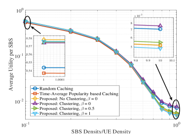
In this section, we analyze the performance of the proposed mechanism and examine insights of the local/global tradeoff ($\beta$) under several deployment and caching scenarios. By assuming a system bandwidth of 1.4MHz, the performance of the proposed scheme is compared against two baseline schemes: random caching (B1) and time-average content popularity based caching (B2). Both baselines and proposed solution uses random RBs to serve usersโ€™ requests. Further, $\frac{\lambda_{\mathrm{SBS}}}{\lambda_{\mathrm{UE}}}=0.1$ denotes a sparse network while $\frac{\lambda_{\mathrm{SBS}}}{\lambda_{\mathrm{UE}}}=1$ denotes a dense network. Fig. 2 shows the per-SBS utility as a function of the ratio of SBS density to user density. With increased $\lambda_{\mathrm{SBS}}/\lambda_{\mathrm{UE}}$, the gains of the proposed scheme ($\beta=0$) vary from 6%-10% and 8%-40% compared to B1 and B2, respectively. Meanwhile, the proposed scheme with clustering ($\alpha=\{0,0.5\}$) achieves 23%, 6% gains over the proposed scheme without clustering.

Refer to caption
Figure 3: Average Utility vs cache size, $C_{f}=50\mathrm{Gbps}$, $\alpha=\beta$

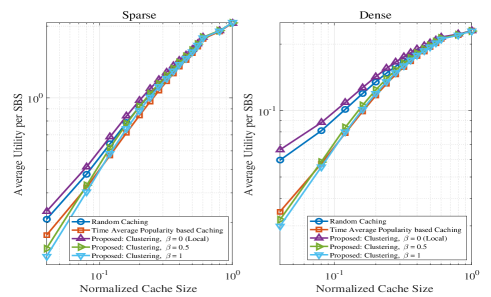
Fig. 3 shows the variation of the per-SBS utility as a function of cache size. For a small cache size, the proposed scheme ($\beta=0$) achieves {10%, 13%} and {25%, 56%} gains over baselines B1 and B2, respectively for {sparse, dense} scenarios. With the increasing cache size, the proposed scheme ($\beta=0$) achieves 7% and 28% gains over baselines B1 and B2 for both scenarios.

Refer to caption
Figure 4: Local/global tradeoff for sparse/dense scenarios, $d$ $=$ $50$, $F$ $=$ $500$
Refer to caption
Figure 5: Local/global tradeoff for sparse/dense scenarios, $d$ $=$ $100$, $F$ $=$ $500$

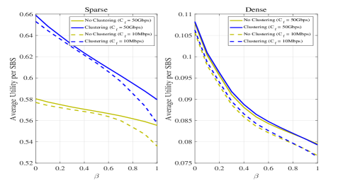
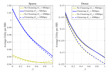
Fig. 4 and 5 shows the tradeoff between local and global learning. It can be observed that the local clustering always performs better than no clustering approach for sparse and dense scenarios. At $\beta=0.8$ for $\mathrm{dense}$ scenario, both schemes yield the same utility for small cache size. Further increasing $\beta$ makes the no clustering approach better than the local clustering. In addition, decreasing the fronthaul capacity has no impact of local/global tradeoff parameter. When the cache size increases, clustering approach is slightly better than non-clustering for dense scenario as shown in Fig. 5. Furthermore, at $\beta=0.7$ for $\mathrm{dense}$ scenario, both schemes yield the utility. By increasing $\beta$ further makes the no clustering approach better than the local clustering. Furthermore, there is no impact of fronthaul capacity on $\beta$.

VI Conclusion

In this letter, we investigated content caching in cloud-aided wireless networks, where SBSs store contents from a large content library. We proposed a clustering algorithm based on Gaussian similarity. Using the regret learning mechanism at the SBSs and the cloud, we proposed a per-SBS caching strategy that minimizes the service delay in serving usersโ€™ requests. In addition, we investigated the tradeoff between local and global content popularity on the proposed algorithm for sparse and dense deployments.

References

  • [1] F. Boccardi et al., โ€œFive disruptive technology directions for 5G, โ€ IEEE Commun. Mag., vol. 52, no. 2, pp. 74 โ€“ 80, Feb. 2014.
  • [2] E. Bastug, M. Bennis, and M. Debbah, โ€œLiving on the edge: The role of proactive caching in 5G wireless networks,โ€ IEEE Commun. Mag., vol. 52, no. 8, pp. 82 โ€“ 89, Aug. 2014.
  • [3] K. Shanmugam et al., โ€œFemtoCaching: wireless video content delivery through distributed caching helpers,โ€ IEEE Trans. Inf. Theory, vol. 59, no. 12, 8402 โ€“ 8413, Dec. 2013.
  • [4] E. Bastug, M. Bennis and M. Debbah, โ€œCache-enabled small cell networks: modeling and tradeoffs, โ€ 11th International Symposium on Wireless Communication Systems (ISWCS), Barcelona, Spain, Aug 2014.
  • [5] B. Chen, C. Yang and A. F. Molisch, โ€œCache-enabled device-to-device communications: offloading gain and energy cost, โ€ 2016 https://arxiv.org/abs/1606.02866.
  • [6] C. Song, Z. Qu, N. Blumm, and A.-L. Barabรกsi, โ€œLimits of predictability in human mobility, โ€ Science, vol. 327, no. 5968, pp. 1018 โ€“ 1021, 2010.
  • [7] M. S. ElBamby, M. Bennis, W. Saad, and M. Latva-aho, โ€œContent-aware user clustering and caching in wireless small cell networks, โ€ 11th International Symposium on Wireless Communication Systems (ISWCS), Barcelona, Spain, Aug 2014.
  • [8] P. Blasco and D. Gunduz, โ€œLearning-based optimization of cache content in a small cell base station, โ€ IEEE International Conference on Communications (ICC), Sydney, Australia, June 2014.
  • [9] Z. Chen and M. Kountouris, โ€œCache-enabled small cell networks with local user interest correlation, โ€ IEEE International Workshop on Signal Processing Advances in Wireless Communications (SPAWC)., Stockhollm, Sweden, June 2015.
  • [10] M. Leconte, M. Lelarge and L. Massoulie, โ€œBipartite graph structures for efficient balancing of heterogeneous load,โ€ in Proc. SIGMETRICS, NewYork, USA, June, 2012.
  • [11] M. Bennis, S. M. Perlaza and M. Debbah, โ€œLearning coarse correlated equilibrium in two-tier wireless networks, โ€ in Proc. IEEE International Conference on Communications (ICC), Ottawa, Canada, June 2012.
  • [12] M. Leconte et al., โ€œPlacing Dynamic Content in Caches with Small Population,ยดยด IEEE INFOCOM, 2016.
  • [13] U. von Luxburg, A tutorial on spectral clustering, Stat. Comput. 17 (4) (2007) 395 โ€“ 416.