Magnetic Response of Magnetospirillum Gryphiswaldense

Abstract

In this study we modelled and measured the U-turn trajectories of individual magnetotactic bacteria under the application of rotating magnetic fields, ranging in ampitude from 1 to $12\text{\,}\mathrm{m}\mathrm{T}$. The model is based on the balance between rotational drag and magnetic torque. For accurate verification of this model, bacteria were observed inside $5\text{\,}\mathrm{\SIUnitSymbolMicro m}$ tall microfluidic channels, so that they remained in focus during the entire trajectory. From the analysis of hundreds of trajectories and accurate measurements of bacteria and magnetosome chain dimensions, we confirmed that the model is correct within measurement error. The resulting average rate of rotation of Magnetospirillum Gryphiswaldense is $0.74\pm 0.03\text{\,}\mathrm{r}\mathrm{a}\mathrm{d}\mathrm{/}\mathrm{m}\mathrm{T}\mathrm{s}$.

I Introduction

Magnetotactic bacteria (MTB) possess an internal chain of magnetosome vesicles Komeili et al. (2004) which biomineralise nanometer sized magnetic crystals (Fe₃O₄ or Fe₃S₄ Lins et al. (2005); Baumgartner and Faivre (2011); Uebe and Schüler (2016)), encompassed by a membrane (magnetosome) Gorby et al. (1988). This magnetosome chain (MC) acts much like a compass needle. The magnetic torque acting on the MC aligns the bacteria with the earth magnetic field Erglis et al. (2007). This is a form of magnetoception Kirschvink et al. (2001), working in conjunction with aero-taxis Frankel et al. (1997). At high latitudes the earth’s magnetic field is not only aligned North-South, but also substantially inclined with respect to the earth’s surface Maus et al. (2010). The MTB are therefore aligned vertically, which converts a three-dimensional search for the optimal (oxygen) conditions into a more efficient one-dimensional search Esquivel and Lins de Barros (1986) (gravitational forces do not play a significant role at the scale of a bacterium). This gives MTB an evolutionary advantage over non-magnetic bacteria in environments with stationary chemical gradients more or less perpendicular to the water surface.

In this paper we address the question of how the MTB of type Magnetosprilillum Gryphiswaldense (MSR-1) respond to varying magnitudes of the external field, in particular a field that is rotating. Even though the response of individual magneto-tactic bacteria to an external magnetic field has been modelled and observed Bahaj and James (1993); Bahaj et al. (1996); van Kampen (1995); Erglis et al. (2007); Cebers (2011), there has been no thorough observation of the dependence on the field strength. The existing models predict a linear relation between the angular velocity of the bacterium and the field strength, but this has not been confirmed experimentally. Nor has there been an analysis of the spread in response over the population of bacteria. The main reason for the absence of experimental data is that the depth of focus at the magnification required prohibits the observation of multiple bacteria in parallel. In this paper, we introduce microfluidic chips with a channel depth of only $5\text{\,}\mathrm{\SIUnitSymbolMicro m}$, which ensures that all bacteria in the field of view remain in focus.

The second motivation for studying the response of MTB to external magnetic fields, is that they are an ideal model system for self propelled medical microrobotics Menciassi et al. (2007); Abbott et al. (2009). Medical microrobotics is a novel form of minimally invasive surgery (MIS), in which one tries to reduce the patient’s surgical trauma while enabling clinicians to reach deep seated locations within the human body Nelson et al. (2004); Abayazid et al. (2013); Felfoul et al. (2016).

The current approach in medical microrobotics is to insert the miniaturized tools needed for a medical procedure into the patient through a small insertion or orifice. By reducing the size of these tools a larger range of natural pathways becomes available. Currently, these tools are mechanically connected to the outside world. If this connection can be removed, so that the tools become untethered, (autonomous) manoeuvring through the veins and arteries of the body becomes possible Dankelman et al. (2011).

If the size and/or application of these untethered systems inside the human body prohibits the storage of energy for propulsion, the energy has to be harvested from the environment. One solution is the use of alternating magnetic fields Abbott et al. (2009). This method is simple, but although impressive progress has been made, it is appallingly inefficient. Only a fraction,  ${10}^{-12}$, of the supplied energy field is actually used by the microrobot. This is not a problem for microscopy experiments, but will become a serious issue if the microrobots are to be controlled deep inside the human body. The efficiency would increase dramatically if the microrobot could harvest its energy from the surrounding liquid. In human blood, energy is abundant and used by all cells for respiration.

For self-propelled objects, only the direction of motion needs to be controlled by the external magnetic field. There is no need for field gradients to apply forces, so the field is allowed to be weaker and uniform when solely using magnetic torque Nelson et al. (2010). Compared to systems that derive their energy for propulsion from the magnetic field, the field can be small in magnitude and only needs to vary slowly. As a result, the energy requirements are low and overheating problems can be avoided.

Nature provides us with a plenitude of self-propelled micro-organisms that derive their energy from bio-compatible liquids, as described first by Bellini Bellini (1963). MTB provide a perfect biokleptic model to test concepts and study the behaviour of self-propelled micro-objects steered by external magnetic fields Khalil et al. (2013).

The direction of the motion of an MTB is modified by the application of a magnetic field at an angle with the easy axis of magnetization of the magnetosome. The resulting magnetic torque causes a rotation of the MTB at a speed that is determined by the balance between the magnetic torque and the rotational drag torque. Under the application of a uniform rotating field, the bacteria follow U-turn trajectories Bahaj and James (1993); Yang et al. (2012); Reufer et al. (2014).

The magnetic torque is often modelled by assuming that the magnetic element is a permanent magnet with dipole moment $\boldsymbol{m}$ [Am²] on which the magnetic field $\boldsymbol{B}$ [T] exerts a torque $\boldsymbol{\Gamma}=\boldsymbol{m}\times\boldsymbol{B}$ [Nm]. This simple model suggest that the torque increases linearly with the field strength, where it is assumed that the atomic dipoles are rigidly fixed to the lattice, and hardly rotate at all. This is usually only the case for very small magnetic fields.

In general one should consider a change in the magnetic energy as a function of the magnetization direction with respect to the object (magnetic anisotropy). This is correctly suggested by Erglis et al. for magnetotactic bacteria Erglis et al. (2007). An estimation of the magnetic dipole moment can be obtained by studying the dynamics of MTB Bahaj et al. (1996).

Recent studies of the dynamics of MTB in a rotating magnetic field show that a random walk is still present regardless of the presence of a rotating field Smid et al. (2015); Cebers (2011). The formation and control of aggregates of MTB in both two- and three-dimensional control systems has been achieved in vitro Martel et al. (2009); Martel and Mohammadi (2010); De Lanauze et al. (2014) as well as in vivo Felfoul et al. (2016), showing that MTB can use the natural hypoxic state surrounding cancerous tissue for targeted drug delivery.

Despite these impressive results, successful control of individual MTB is much less reported. This is because many experiments suffer from a limited depth of focus of the microscope system, leading to a loss of tracking. A collateral problem is overheating of the electromagnets in experiments that take longer than a few minutes. We recently demonstrated the effect of varying field strengths on the control of magneto-tactic bacteria Hassan et al. (2016). In the present paper we provide the theoretical framework and systematically analyse the influence of the magnetic field on the trajectories of individual MTB. This knowledge will contribute to more efficient control of individual MTB, and ultimately self-propelled robotic systems in general.

We present a thorough theoretical analysis of the magnetic and drag torques on MTB. This model is used to derive values for the proportionality between the average rate of rotation and the magnetic field during a U-turn trajectory under a magnetic field reversal. The theory is used to predict U-turn trajectories of MTB, which are the basis for our experimental procedures.

Lastely, we present statistically significant experimental results which verify our theoretical approach and employ a realistic range of magnetic field strength and rotational speed of the applied magnetic field to minimize energy input.

II Theory

II.1 The Rate of Rotation

II.1.1 The dependence on the field

The magnetic torque $\Gamma$ [Nm] is equal to the change in total magnetic energy $U$ [J] with changing applied field angle. We consider only the demagnetization and external field energy terms. The demagnetization energy is caused by the magnetic stray field $\boldsymbol{H}_{\text{d}}$ [A/m] that arises due to the magnetosome magnetization $\boldsymbol{M}$ [A/m]. In principle, one has to integrate the stray field over all space. Fortunately, this integral is mathematically equivalent to Hubert and Schäfer (1998)

$$U_{\text{d}}=\textstyle{\frac{1}{2}}\mu_{0}\int\boldsymbol{M}\cdot\boldsymbol{H_{\text{d}}}\text{d}V,$$ (1)

with $\mu_{o}$ the vacuum permeability, $4\pi 10^{-7}$. In this formulation, the integral is conveniently restricted to the volume $V$ of the magnetic material.

The demagnetization energy acts to orient the magnetization so that the external stray field energy is minimized. We can define a shape anisotropy term $K$ [J/m³] to represent the energy difference between the hard and easy axes of magnetization, which are perpendicular to each other,

$$K=\left(U_{\text{d, max}}-U_{\text{d, min}}\right)/V.$$ (2)

The external field energy is caused by the externally applied field $\boldsymbol{H}$ [A/m]

$$U_{\text{H}}=-\mu_{0}\int\boldsymbol{M}\cdot\boldsymbol{H}\text{d}V,$$ (3)

and acts to align $\boldsymbol{M}$ parallel to $\boldsymbol{H}$. Assuming that the magnetic element of volume $V$ is uniformly magnetized with saturation magnetization $M_{\text{s}}$ [A/m], the total energy can then be expressed as

$$U=KVsin^{2}(\theta)-\mu_{0}M_{\text{s}}HVcos(\varphi-\theta).$$ (4)

The angles $\theta$ and $\varphi$ are defined as in figure 1. Normalizing the energy, field, and torque by

$$u =\nicefrac{{U}}{{KV}}$$ (5)

$$h =\nicefrac{{\mu_{0}HM}}{{2K}}$$ (6)

$$\tau =\nicefrac{{\Gamma}}{{KV}},$$ (7)

respectively, the expression for the energy can be simplified to

$$u=\sin^{2}(\theta)-2h\cos(\varphi-\theta).$$ (8)

Figure 1: Definition of the field angle $\varphi$ and the magnetization angle $\theta$ between the easy axis $K$, the magnetization $M$ and the magnetic field $H$.

The equilibrium magnetization direction is reached for $\nicefrac{{\partial u}}{{\partial\theta}}=0$. The solution for this relationship cannot be expressed in an analytically concise form. The main results are however that for $h<\nicefrac{{1}}{{\sqrt{2}}}$, the maximum torque is reached at the field angle $\varphi_{\text{max}}=\nicefrac{{\pi}}{{2}}$,

$$\tau_{\text{max}} =2h\sqrt{1-h^{2}} \text{ for }h\leq\nicefrac{{1}}{{\sqrt{2}}}$$ (9)

$$=1 \text{ for }h>\nicefrac{{1}}{{\sqrt{2}}}.$$ (10)

The angle of magnetization at maximum torque can be approximated by

$$\theta_{\text{max}}=h+0.1h^{2}\text{ for }h<\nicefrac{{1}}{{\sqrt{2}}},\\$$ (11)

where the error is smaller than $5\times 10^{-3}$ rad ($1.6\text{\,}\mathrm{\SIUnitSymbolDegree}$) for $h<0.5$.

For $h>1$, the field angle $\varphi_{\text{max}}$ at which the maximum torque is reached is smaller than $\nicefrac{{\pi}}{{2}}$ and approaches $\nicefrac{{\pi}}{{4}}$ for $h\rightarrow\infty$. This behaviour can be very well approximated by

$$\varphi_{\text{max}}=\frac{\pi}{4}\left(1+\frac{2}{3h}\right)\text{ for }h>1,$$ (12)

where the error is smaller than $3\times 10^{-3}\pi$ ($0.5\text{\,}\mathrm{\SIUnitSymbolDegree}$).

In summary, and returning to variables with units, the maximum torque is $\Gamma_{\text{max}}=KV$, which is reached at

$$H>\frac{\sqrt{2}K}{\mu_{0}M_{\text{s}}}$$ (13)

at an angle $\varphi=\nicefrac{{\pi}}{{2}}$, which, to a good approximation, decreases linearly with $1/H$ to $\varphi=\nicefrac{{\pi}}{{4}}$ at an infinite external field.

II.1.2 Demagnetization factor

The magnetization $M_{\text{s}}$ is a material parameter, so the only variable to be determined is the magnetosome’s demagnetization factor. As a first approximation, we can consider the chain of magnetic crystals in the magnetosome as a chain of $n$ dipoles separated at a distance $a$, each with a dipole moment $m$=$M_{s}V$ [Am²], where $V$ is the volume of each single sphere. We assume that all dipoles are aligned parallel to the field ($\varphi=\theta$) to obtain an upper limit on the torque. (See figure 1 for the definition of the angles). The magnetic energy for such a dipole chain has been derived by Jacobs and Bean Jacobs and Bean (1955), which, rewritten in SI units, is

$$U= \frac{\mu_{0}m^{2}}{4\pi a^{3}}nK_{n}\left(1-3\cos^{2}(\theta)\right)+$$

$$\mu_{0}nmHcos(\varphi-\theta)$$ (14)

$$K_{n}= \sum_{j=1}^{n}\frac{(n-j)}{nj^{3}}.$$ (15)

The maximum torque equals the energy difference between the state where all moments are parallel to the chain ($\theta$=0) and the state where they are perpendicular to the chain ($\theta$=$\pi/2$), under the condition that the angle between the moments and the field is zero:

$$\Gamma_{\text{max}} =\frac{3\mu_{0}m^{2}}{4\pi a^{3}}nK_{n}.$$ (16)

For a single dipole $n=1$, $K_{n}$=0 and there is no energy difference, as expected.

Combined with equations (6) and (9), and re-introducing units, the field dependent torque becomes

$$\Gamma =\Gamma_{\text{max}}2h\sqrt{1-h^{2}}\text{ with }$$ (17)

$$h =\frac{H}{\Delta NM_{\text{s}}}.$$ (18)

The magnetosome does not consist of point dipoles but should be approximated by spheres with radius $r$, spaced at a distance of $a$ from each other (figure 2). We can modify the Jacob and Bean model by introducing the volume of a single sphere $V$ and the magnetization $M_{s}$ of the magnetite crystal ($4.8\text{\times}{10}^{5}\text{\,}\mathrm{A}\mathrm{/}\mathrm{m}$ Witt et al. (2005)),

$$\Gamma_{\text{max}}=\frac{1}{2}\mu_{0}M_{s}^{2}nV\Delta N$$ (19)

$$\Delta N=2K_{n}\left(\frac{r}{a}\right)^{3},$$ (20)

as a correction to equation 16. This correction is based on the fact that the field of a uniformly magnetized sphere is identical to a dipole field Griffiths (1999) outside the sphere, and the average of the magnetic field over a sphere not containing currents is identical to the field at the center of that sphere Hu (2000, 2008).

For an infinitely long chain of touching spheres, $d$=0 and $n\rightarrow\infty$, the difference in demagnetization factors ($\Delta N$) approaches $0.3$ (Figure 3). Approximating the chain by a long cylinder ($\Delta N$=0.5) Hanzlik et al. (1996); Erglis et al. (2007) therefore overestimates the maximum torque by 40%. Simply taking the total magnetic moment to calculate the torque, as if $\Delta N$=1, would overestimate it by a factor of three.

Figure 2: Chain of magnetic spheres of radius $r$, spaced at a distance $d$, approximated by point dipoles spaced by a distance $a=r+d$, magnetized along the longitudinal axis of the chain (top) or perpendicular to its longitudinal axis (bottom).

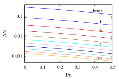
Figure 3: Difference in demagnetization factors of a chain of spheres as function of number of spheres $n$ for varying spacing between the spheres $d/r$.

II.1.3 Low field approximation

For low values of the field ($h\ll 1$), equation (16) can be approximated by

$$\Gamma\approx\Gamma_{\text{max}}2h=\mu_{0}M_{\text{s}}nVH=mB,$$ (21)

where $m$ [$\mathrm{A}\mathrm{m}^{2}$] is the total magnetic moment of the magnetosome chain and assuming the permeability of the medium to be equal to vacuum. This approximation is commonly used in the field of MTB studies. Based on the theory presented here, it is now possible to estimate up to which field value this is approximation is valid.

The normalization to the reduced field $h$ is solely dependent on the magnetization and demagnetization factors of the chain. Based on the values for magnetosome morphology (table 1), we can estimate the field dependence of the torque. Figure 4 shows the torque as a function of the field for the range of values tabulated, normalized to the maximum torque. Also shown is the approximation for the case when the magnetization remains aligned with the easy axes. For Magnetospirillum Gryphiswaldense, the linear range is valid up to fields of about $10\text{\,}\mathrm{m}\mathrm{T}$ for $90\text{\,}\mathrm{\char 37\relax}$ of the population.

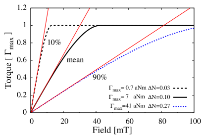
Figure 4: Magnetic torque on magnetotactic bacteria, normalized to the maximum torque, as a function of applied field for the average of the population, as well as the $10\text{\,}\mathrm{\char 37\relax}$ and $90\text{\,}\mathrm{\char 37\relax}$ cut-off (see table 1). The red solid asymptotes show the linear approximation for $\Gamma=mB$.

II.1.4 Drag torque

Magnetotactic bacteria are very small, and rotate at a few revolutions per second only. Inertial forces therefore do not play a significant role. The ratio between the viscous and inertial forces is characterized by the Reynolds number $Re$, which for rotation at an angular velocity of $\omega$ [rad/s] is

$$Re=\frac{L^{2}\rho\omega}{4\eta},$$ (22)

where $L$ is the characteristic length (in our case, the length of the bacterium), $\rho$ the density, and $\eta$ the dynamic viscosity of the liquid (for water, these are, respectively, ${10}^{3}\text{\,}\mathrm{k}\mathrm{g}\mathrm{/}\mathrm{{}^{3}}\mathrm{m}$, and $1\text{\,}\mathrm{m}\mathrm{P}\mathrm{a}\mathrm{s}$). Experiments by Dennis et al. Dennis et al. (1980) show that a Stokes flow approximation for the drag torque is accurate up to $Re$=$10$. In experiments with bacteria, the Reynolds number is on the order of ${10}^{-3}$ and the Stokes flow approximation is certainly allowed. The drag torque is therefore simply given by

$$\Gamma_{\textrm{D}}=f_{\text{b}}\omega,$$ (23)

The rotational drag coefficient of the bacterium, $f_{\text{b}}$, needs to be estimated for the type of MTB studied. In a first approximation, one could consider the MTB to be a rod of length $L$ and diameter $W$. Unfortunately, there is no simple expression for the rotational drag of a cylinder. Dote Dote and Kivelson (1983) gives a numerical estimate of the rotational drag of a cylinder with spherical caps (spherocylinder). Fortunately, for typical MSR-1 dimensions, it can be shown that a prolate spheroid of equal length and diameter has a rotational drag coefficient that is within $10\text{\,}\mathrm{\char 37\relax}$ of that value. To a first approximation, one can therefore assume the rotational drag of an MSR-1 to be given by Berg (1993)

$$f_{\text{e}}=\frac{\pi\eta L^{3}}{3\ln\left(\frac{2L}{W}\right)-\frac{3}{2}}.$$ (24)

However, the MSR-1 has a spiral shape, so the actual drag will be higher. Rather than resorting to complex finite element simulations, we chose to empirically determine the rotational drag torque by macroscopic experiments with 3D printed bacteria models in a highly viscous medium (Section III.4.). We introduce a bacteria shape correction factor $\alpha_{\text{bs}}$ to the spheroid approximation, which is independent of the ratio $L/W$ over the range of typical values for MSR-1 and has a value of about $1.65$. The corrected rotational drag coeffient for the bacteria then becomes

$$f_{\textrm{b}}=\alpha_{\text{bs}}f_{\textrm{e}}.$$ (25)

II.1.5 Diameter and duration of the U-turn

At the steady-state rate, the magnetic torque is balanced by the rotational drag torque, leading to a rate of rotation of

$$\omega=\frac{\Gamma}{f_{\text{b}}}\approx\frac{mB\sin\phi(t)}{f_{\text{b}}}.$$ (26)

The approximation is for low field values (see figure 4), in which case $\phi$ is the angle between the applied field and the long axis of the bacteria (magnetosome).

The maximum rate of rotation, $mB/f_{\text{b}}$, is obtained when the field is perpendicular to the long axis of the bacteria. Suppose that we construct a control loop to realize this condition over the entire period of a U-turn. Then the minimum diameter and duration of this loop would be

$$D_{\text{min}} =\frac{2f_{\text{b}}v}{mB}$$ (27)

$$T_{\text{min}} =\frac{\pi f_{\text{b}}}{mB},$$ (28)

where $D_{\text{min}}$ is the minimum size of a U-turn’s diameter and $T_{\text{min}}$ is the minimum time of a U-turn. On the other hand, if we reverse the field instantaneously, the torque will vary over the trajectory of the U-turn. Compared to the situation above, the diameter of the U-turn increases by a factor of $\nicefrac{{\pi}}{{2}}$:

$$D=\frac{\pi f_{\text{b}}v}{mB}.$$ (29)

The diameter of the U-turn increases with the velocity of the bacterium. To obtain a description that only depends on the dimensions of the bacteria, we introduce a new parameter $v/D$ [$\mathrm{r}\mathrm{a}\mathrm{d}\mathrm{/}\mathrm{s}$], which can be interpreted as an average rate of rotation. The relation between the average rate of rotation and the magnetic field $B$ is

$$\frac{v}{D}=\gamma B,$$ (30)

where the proportionality factor $\gamma$ [$\mathrm{r}\mathrm{a}\mathrm{d}\mathrm{/}\mathrm{T}\mathrm{s}$] can be linked to the bacterial magnetic moment $m$ and drag coefficient $f_{\text{b}}$ [$\mathrm{N}\mathrm{m}\mathrm{s}$],

$$\gamma=\frac{m}{\pi f_{\text{b}}}.$$ (31)

Note, however, that this expression is only valid in the low field approximation.

The determination of the duration of the U-turn trajectory is complicated by the fact that the magnetic torque starts and ends at zero (at $\theta$=0 or $\pi$). In this theoretical situation, the bacteria would never turn at all. Esquivel et al. Esquivel and Lins de Barros (1986) solve this problem by assuming a disturbance acting on the motion of the bacteria. This disturbance could be due to Brownian motion, as used by Esquivel et al., or due to flagellar propulsion, as we use in the simulations in the following section. Assuming an initial disturbing angle of $\theta_{\text{i}}$, the duration $T$ [s] of the U-turn becomes

$$T=\frac{2f_{\text{b}}}{mB}\ln\frac{2}{\theta_{\text{i}}}.$$ (32)

II.2 U-turn Trajectory Simulations

To check the validity of the analytical approach, we performed simulations. The MTB are approximated by rigid magnetic dipoles with constant lateral velocity $v$ at an orientation of $\theta_{x}(t)$ and angular velocity of $\omega(t)$ (see figure 5). They are subject to a magnetic field with magnitude $B$ at an orientation of $\varphi_{x}(t)$, resulting in a magnetic torque of $\Gamma(t)$. In contrast to the analytical model, it is assumed that flagellar motion causes an additive sinusoidal torque $\Gamma_{\text{f}}(t)$ with amplitude $A_{\text{f}}$ and angular velocity $\omega_{\text{f}}$. These should be in balance with the drag torque: $\Gamma_{\text{D}}=f_{\text{b}}\omega(t)$. The following set of equations link the physical model to the coordinates $x(t)$, $y(t)$:

Figure 5: Bacterium at angle $\theta_{x}$ with magnetic field at angle $\varphi_{x}$.

$$x(t) = x(0)+\int_{0}^{t}v\cos(\theta_{x}(t))\text{d}t$$ (33)

$$y(t) = y(0)+\int_{0}^{t}v\sin(\theta_{x}(t))\text{d}t$$ (34)

$$\theta_{x}(t) = \theta_{x}(0)+\int_{0}^{t}\omega(t)\text{d}t$$ (35)

$$\omega(t) = \frac{1}{f_{\text{b}}}\left(\Gamma_{\text{mag}}(t)+\Gamma_{\text{flag}}(t)\right)$$ (36)

$$= \frac{mB}{f_{\text{b}}}\sin(\varphi_{x}(t)-\theta_{x}(t))+\frac{A_{\text{f}}}{f_{\text{b}}}\sin(\omega_{\text{f}}t)$$ (37)

A linear, closed-form solution of the diameter of the trajectory of the U-turn in the case of an instantaneous field reversal and no flagellar torque is given by equation 29. This solution is not valid, however, in the case of slowly rotating fields. The experimental magnetic field is considered to rotate according to a constant-acceleration model with a total rotation period of $130\text{\,}\mathrm{m}\mathrm{s}$ (see section III.4). Simulations were carried out with time steps of $10\text{\,}\mathrm{\SIUnitSymbolMicro s}$, which is comfortably fast and precise (decreasing this to $1\text{\,}\mathrm{\SIUnitSymbolMicro s}$ changes the results by approximately $0.01\text{\,}\mathrm{\char 37\relax}$). Figure 6 shows several simulated trajectories subject to fields of various magnitudes, assuming nonzero flagellar torque and realistic MTB parameters.

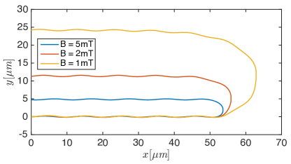
Figure 6: Simulated trajectories assuming flagellar torque and a non-instantaneously rotating field for several values of the magnetic field magnitude $B$. The time step of the simulation is $10\text{\,}\mathrm{\SIUnitSymbolMicro s}$

Figure 7 shows the simulated $\nicefrac{{v}}{{D}}$ as a function of the field magnitude. It can be seen that during an instantaneous field reversal, the solution is nearly identical to the closed-form solution of equation 29. The difference is caused by the influence of flagellar torque. Introducing a field reversal time $T_{\text{mag}}$ of $130\text{\,}\mathrm{m}\mathrm{s}$ into a continuous-acceleration model significantly changes the profile, yielding a similar result for low fields, increasing at moderate fields, and saturating to a maximum value of $16.6\text{\,}\mathrm{s}^{-1}$. $B_{\text{opt}}$ is defined as the field magnitude at which $\nicefrac{{v}}{{D}}$ has the largest difference from the theoretical curve. Figure 8 shows, from simulations, that the optimal reversal time is inversely proportional to the magnetic field strength. For fields below $B_{\text{opt}}$, $\nicefrac{{v}}{{D}}$ can be considered linear with a maximum nonlinearity error of $2\text{\,}\mathrm{\char 37\relax}$, independently of $T_{\text{mag}}$.

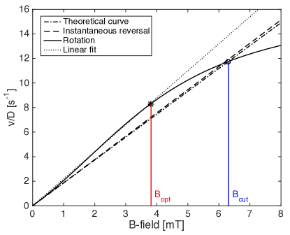
Figure 7: Simulated values of $v/D$ for different rotation speeds of the magnetic field, with (red) and without (blue) and flagellar torque, compared with the linear model proposed by Erglis et al. Erglis et al. (2007) (dotted line).

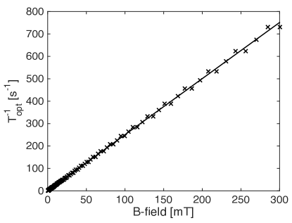
Figure 8: Simulated optimum reversal time of the magnetic field as a function of the field strength.

III Experimental

III.1 Magnetotactic bacteria cultivation

A culture of Magnetospirillum Gryphiswaldense was used for the magnetic moment study. The cultures were inoculated in MSGM medium ATCC 1653 according to with an oxygen concentration of $15\text{\,}\mathrm{\char 37\relax}$. The bacteria were cultivated at $21\text{\,}\mathrm{\SIUnitSymbolCelsius}$ for $25\text{\,}\mathrm{d}\mathrm{a}\mathrm{y}\mathrm{s}$ for optimal chain growth Katzmann et al. (2013). The sampling was done using a magnetic “racetrack” separation, as described in  Wolfe et al. (1987).

III.2 Dynamic viscosity of growth medium

The kinematic viscosity of the freshly prepared growth medium was determined with an Ubbelohde viscometer with a capillary diameter of $0.63\pm 0.01\text{\,}\mathrm{m}\mathrm{m}$ (Si Analytics 50110). The viscometer was calibrated with deionized water, assuming it has a kinematic viscosity of $0.98\pm 0.01\text{\,}\mathrm{m}\mathrm{m}^{2}\mathrm{/}\mathrm{s}$ at $21.0\pm 0.5\text{\,}\mathrm{\SIUnitSymbolCelsius}$. At that temperature, the growth medium has a kinematic viscosity of $0.994\pm 0.017\text{\,}\mathrm{m}\mathrm{m}^{2}\mathrm{/}\mathrm{s}$. The density of the growth medium was $1.009\pm 0.002\text{\,}\mathrm{g}\mathrm{/}\mathrm{c}\mathrm{m}^{3}$, measured by weighing $1\text{\,}\mathrm{m}\mathrm{l}$ of it on a balance. The dynamic viscosity of the growth medium is therefore $1.004\pm 0.019\text{\,}\mathrm{m}\mathrm{P}\mathrm{a}\mathrm{s}$, which is, within measurement error, identical to water ($1.002\text{\,}\mathrm{m}\mathrm{P}\mathrm{a}\mathrm{s}$).

III.3 Microfluidic Chips

Microfluidic chips with a channel depth of $5\text{\,}\mathrm{\SIUnitSymbolMicro m}$ were constructed by lithography, HF etching in glass and subsequent thermal bonding. The fabrication process is identical to the one described in Park et al. (2015). Figure 9 shows the resulting structures, consisting of straight channels with inlets on both sides. By means of these shallow channels, the MTBs are kept within the field of focus during microscopic observation, so as to prevent out-of-plane focus while tracking. The channel width was $200\text{\,}\mathrm{\SIUnitSymbolMicro m}$ or more, so that the area over which U-turns could be observed was only limited by the field of view of the microscope.

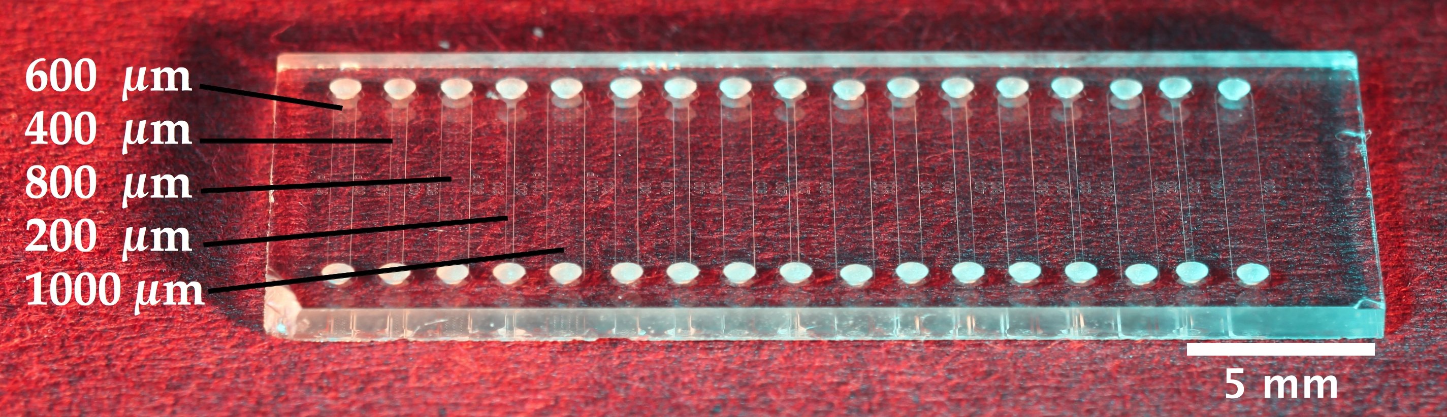
Figure 9: Top: A $5\text{\,}\mathrm{\SIUnitSymbolMicro m}$ deep microfluidic chip with various channel widths of 200, 400, 600, 800 and 1000 $\mathrm{\SIUnitSymbolMicro m}$.

III.4 Magnetic Manipulation Setup

A schematic of the full setup, excluding the computer used for the acquisition of the images, is shown in figure 10. A permanent NdFeB magnet ($5\text{\times}5\text{\times}10\text{\,}\mathrm{m}\mathrm{m}$, grade N42) is mounted on a stepper motor (Silverpak 17CE, Lin Engineering) below the microfluidic chip. The direction of the field can be adjusted with a precision of $51\,200$ steps for a full rotation, at a rotation time of $130\text{\,}\mathrm{m}\mathrm{s}$ with a constant acceleration of $745\text{\,}\mathrm{r}\mathrm{a}\mathrm{d}\mathrm{s}^{-2}$. The field strength is adjusted using a labjack, with a positioning accuracy of $0.5\text{\,}\mathrm{m}\mathrm{m}$.

The data acquisition was done by a Flea3 digital camera ($1328$$\times$$1048$ at $100\text{\,}\mathrm{f}\mathrm{p}\mathrm{s}$, FL3-U3-13S2M-CS, Point Grey) mounted on a Zeiss Axiotron 2 microscope with a $20$$\times$ objective.

During the experiments, a group of MTB was observed while periodically (every two seconds) rotating the magnetic field. This was recorded for field magnitudes ranging from $112\text{\,}\mathrm{m}\mathrm{T}$. Offline image processing techniques were used to track the bacteria and subtract their velocity and U-turn diameter.

Figure 10: The setup used to measure the MTB U-turns. (a) Reflective microscope, (b) microfluidic chip and (c) a permanent magnet mounted on (d) a stepper motor.

Knowing the error in our measurements of the magnetic field is fundamental to determining the responsiveness of the MTB. Therefore we measured the magnetic fields at specific heights using a Hall meter (Metrolab THM1176). The results can be seen in figure 11.

Figure 11: Magnetic field strength as a function of distance of the magnet to the microfluidic chip.

The placement of the tip of the Hall meter was at the location of the microfluidic chip, assuming the field strength inside the chip’s chamber equals that at the tip. It should be noted that the center of the magnet was aligned with the center of rotation of the motor, therefore the measurements were only done with a stationary magnet on top of an inactive motor. Errors in the estimation of the magnetic field strength due to misalignment of the magnetic center from our measurements therefore cannot be excluded.

The rotation profile of the motorized magnet was investigated by recording its motion by a digital camera at $120\text{\,}\mathrm{f}\mathrm{p}\mathrm{s}$ and evaluating its time-dependent angle by manually drawing tangent lines. Figure 12 shows that the profile accurately fits a constant-acceleration model with an acceleration of $745\text{\,}\mathrm{r}\mathrm{a}\mathrm{d}\mathrm{s}^{-2}$, resulting in a total rotation time of $130\text{\,}\mathrm{m}\mathrm{s}$.

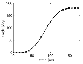
Figure 12: The measured angle of the motorized magnet accurately fits a constant-acceleration model with a total rotation period of $130\text{\,}\mathrm{m}\mathrm{s}$.

III.5 Macroscopic Drag Setup

Macro-scale drag measurements were performed using a Brookfield DV-III Ultra viscometer. During the experiment, we measured the torque required to rotate different centimeter sized models of bacteria and simple shapes in silicone oil (Figure 13). In order to keep the Reynolds number less than one, silicone oil of $5000\text{\,}\mathrm{m}\mathrm{P}\mathrm{a}\mathrm{s}$ (Calsil IP 5000 from Caldic, Belgium) was used as a medium to generate enough drag. Furthermore, the parts were rotated at speeds below $30\text{\,}\mathrm{r}\mathrm{p}\mathrm{m}$. The models were realized by 3D printing. The designs can be found in the accompanying material.

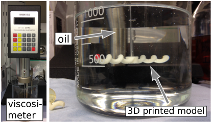
Figure 13: The viscometer setup used to measure the rotational drag of macroscopic spheroid and helical structures. 3D printed models were mounted on a shaft and rotated in a high viscosity silicone oil ($5\text{\,}\mathrm{P}\mathrm{a}\mathrm{s}$). A video of the experiment is available as additional material (DragMeasurements.mp4).

III.6 Image Processing

The analysis of the data was done using in-house detection and tracking scripts written in MATLAB^®. The process is illustrated in figure 14. In the detection step, static objects and non-uniform illumination artefacts are removed by subtracting a background image constructed by averaging 30 frames spread along the video. High-frequency noise is reduced using a Gaussian lowpass filter. A binary image is then obtained using a thresholding operation, followed by selection on a minimum and maximum area size. The centers-of-mass of the remaining blobs are compared in subsequent frames, and woven to trajectories based on a nearest-neighbor search within a search radius 14. A sequence of preprocessing steps can be seen in figure 15. The software used is available under additional material.

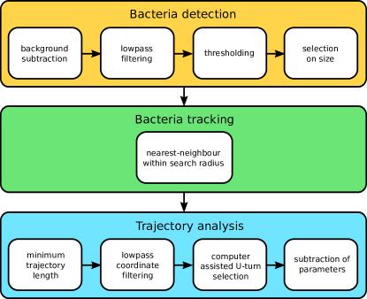
Figure 14: The process of bacteria detection, tracking, and subsequent analysis.

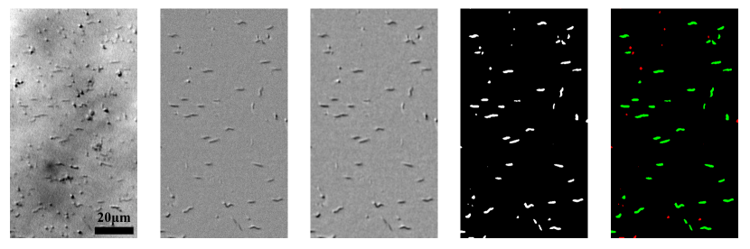
Figure 15: Pre-processing filter steps: (a) raw, (b) background subtraction, (c) low pass filtering, (d) thresholding resulting in a binary image, (e) size selectivity. A video is available as additional material ($MTB\_imageProc.mp4$)

Subsequently, the post-processing step involves the semi-automated selection of the MTB trajectories of interest for the purpose of analysis. The U-turn parameters of interest analyzed are the velocity $v$, the diameter $D$ of the U-turn, and the time $t$. A typical result of the post-processing step can be seen in figure 16.

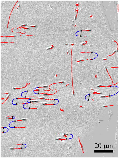
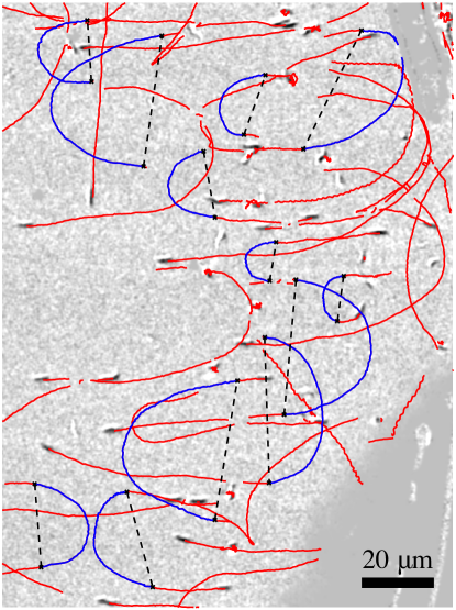
Figure 16: Trajectory during image post-processing at a magnetic field strength of $12.2\text{\,}\mathrm{mT}$ (left) and $1.5\text{\,}\mathrm{mT}$ (right). Selection procedure of analyzed U-turns, showing selected U-turns in blue and unanalyzed trajectories in red. The black dotted line connects two manually selected points of a given U-turn trajectory, from which the distance in the $y$-direction, or the U-turn diameter, is determined.

IV Results and discussions

The model developed in section II predicts the trajectories of MTB under a changing magnetic field: in particular, the average rate of rotation over a U-turn. To validate the model, the essential model parameters are determined in section IV.1, after which the average rate of rotation is measured and compared to theory in section IV.2.

IV.1 Estimate of model parameters

The rate of rotation of an MTB under a rotating magnetic field is determined by the ratio between the rotational drag torque and the magnetic torque. Both will be discussed in the following, after which the average rate of rotation will be estimated.

IV.1.1 Estimate of rotational drag torque

To determine the rotational drag torque, the outer shape of the MTB was measured by both optical microscopy and scanning electron microscopy (SEM). The drag coefficient was estimated from a macroscale drag viscosity measurement.

Outer dimensions of the bacteria

The length $L$ of the bacteria is measured from the same optical images as used for the trajectory analysis (figures 16). Scanning electron microscopy (SEM) would in principle give higher precision per bacterium, but due to the lower number of bacteria per image the estimate of the average length and distribution would have a higher error. Moreover, using the video footage ensures that the radius of curvature and the length of the bacteria are measured on the same bacterium.

A typical MTB has a length of $5.0\pm 0.2\text{\,}\mathrm{\SIUnitSymbolMicro m}$. The length distribution is shown in Figure 18. These values agree with values reported in the literature Schleifer et al. (1991); Bazylinski and Frankel (2004); Faivre et al. (2010).

The width $W$ of the bacteria is too small to be determined by optical microscopy, and needs to be determined from SEM images, see figure 17. A typical bacterium has a width of $240\pm 6.\text{\,}\mathrm{n}\mathrm{m}$. The main issue with SEM images is whether a biological structure is still intact or perhaps collapsed due to dehydration, which might cause overestimation of the width. The latter might be as high as $\nicefrac{{\pi}}{{2}}$ if the bacterial membrane has completely collapsed. Fortunately, the drag coefficient scales much more strongly with the length than with the width (equation 24). For a typical bacterium, the overestimation of the width by using SEM leads at most to an overestimation of the drag by $18\text{\,}\mathrm{\char 37\relax}$.

Table 1 lists the values of the outer dimensions $L$ and $W$, including the measurement error and standard deviation over the measured population.

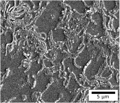
Figure 17: Scanning electron microscopy images of Magnetospirillum Gryphiswaldense. Separated MTB were selected for width measurements.

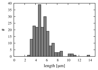
Figure 18: Number of magnetotactic bacteria (MTB) as a function of the length of the MTB as measured by optical microscopy.

Rotational Drag

From the outer dimensions of the bacteria, the rotational drag torque can be estimated. The bacterial shape correction factor, equation (25), was determined by macro-scale experiments with 3D printed models of an MTB in a viscosimeter using high viscosity silicone oil (see section III.5). Figure 19 shows the measured torque as a function of the rotational speed for prolate spheroids and spiral shaped 3D printed bodies of two different lengths. The relation between the torque and the speed is linear, so we are clearly in the laminar flow regime. This is in agreement with an estimated Reynolds number of less than $0.3\text{\,}$ for this experiment (equation 22). Independently of the size, the spiral shaped MTB models have a drag coefficient that is $1.64\pm 0.05\text{\,}$ times higher ($\alpha_{\text{BS}}$) than that of a spheroid of equal overall length and diameter.

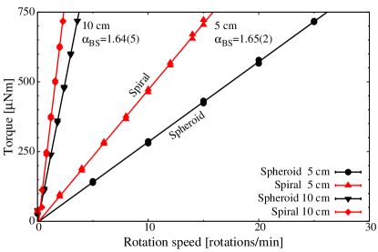
Figure 19: Rotational drag torque versus angular rotation speed of 3D printed prolate spheroids and MTB models of lengths $5$ and $10\text{\,}\mathrm{c}\mathrm{m}$. The curves are linear, indicating that the flow around the objects is laminar. Irrespective of the length, the spiral shaped MTB model has a drag that is $1.64\pm 0.05\text{\,}$ higher than a prolate spheroid of equal overall length and diameter.

Using the same experimental configuration, we can obtain an estimate of the effect of the channel walls on the rotational drag by changing the distance between the 3D printed model and the bottom of the container. Figure 20 shows the relative increase in drag when the spiral shape approaches the wall. This experiment was performed on a $5\text{\,}\mathrm{c}\mathrm{m}$ long, $5\text{\,}\mathrm{m}\mathrm{m}$ diameter spiral at $8\text{\,}\mathrm{r}\mathrm{p}\mathrm{m}$. To visualise the increase, the reciprocal of the distance normalised to the length of the bacteria is used on the bottom horizontal axis. The normalised length is shown on the top axes. Note that when plotted in this way, the slope approaches unity at larger distances.

For an increase over $5\text{\,}\mathrm{\char 37\relax}$, the model has to approach the wall at a distance smaller than $L$/3, where $L$ is the length of the bacteria. For very long bacteria of $10\text{\,}\mathrm{\SIUnitSymbolMicro m}$, this distance is already reached in the middle of the $5\text{\,}\mathrm{\SIUnitSymbolMicro m}$ high channel. Since there are two channel walls on either side at the same distance, we estimate that the additional drag for bacteria swimming in the centre of the channel is less than $15\text{\,}\mathrm{\char 37\relax}$. If the spiral model approaches the wall, the drag rapidly increases. At $L/50$, the drag increases by $60\text{\,}\mathrm{\char 37\relax}$. It is tempting to translate this effect to real MTB. It should be noted however that the 3D printed models are rigid and stationary, whereas the MTB are probably more flexible and mobile. Intuitively, one might expect a lower drag.

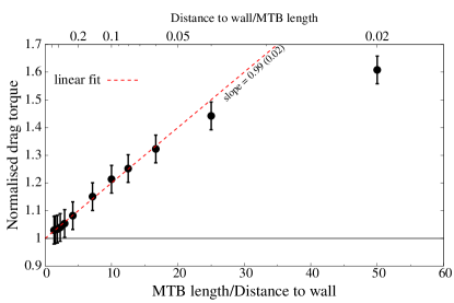
Figure 20: Increase in rotational drag as a function of the distance between the 3D printed spiral and the bottom of the container. The distance is normalized to the length of the bacteria ($5\text{\,}\mathrm{c}\mathrm{m}$). The torque is normalized to the extrapolated value for infinite distance (displayed as “linear fit”).

From the bacterial dimensions, we can estimate a mean rotational drag coefficient, $f_{\text{b}}$, of $67\pm 7.\text{\,}\mathrm{z}\mathrm{N}\mathrm{s}$. Since the relation between the rotational drag and the bacterial dimensions is highly nonlinear, a Monte Carlo method was used to estimate the error and variation of $f_{\text{b}}$. For these calculations, the length of the bacteria was assumed to be Gaussian distributed with parameters as indicated in table 1. The code for the Monte Carlo calculation is available as additional material.

Due to the nonlinearity, the resulting distribution of $f_{\text{b}}$ is asymmetric. So rather than the standard deviation, the $1090\text{\,}\mathrm{\char 37\relax}$ cut-off values of the distribution are given in table 2). Most of the MTB are estimated to have a drag coefficient in the range of $30$ to $120\text{\,}\mathrm{z}\mathrm{N}\mathrm{s}$.

Table 1: Characteristics of magnetotactic bacteria. Length $L$ and width $W$ and amount $n$, diameter $d$ and spacing $a$ of the crystals in the magnetosomes. The error indicated on the means is the standard error (standard deviation/square root of the total number of samples).

	$L$	$W$	$n$	$d$	$a$
	[$\mathrm{\SIUnitSymbolMicro}\mathrm{m}$]	[nm]		[nm]	[nm]
mean	$5.0\pm 0.2$	$240\pm 6.$	$16\pm 2.$	$40\pm 2.$	$56\pm 1.$
stddev	1	28	6	9	8

Table 2: From the values of table 1, the drag coefficient $f_{\text{r}}$, demagnetisation factors $\Delta N$, magnetic moment $m$, maximum magnetic torque $\Gamma_{\text{max}}$, and proportionality factor $\gamma$ are estimated ($v/D=\gamma B$). The input parameters are assumed to obey a Gaussian distribution with standard deviations as in table 1. Using a Monte Carlo method, the standard error of the calculated parameters, and the $10\text{\,}\mathrm{\char 37\relax}$–$90\text{\,}\mathrm{\char 37\relax}$ cut-offs in the distribution, are calculated.

	$f_{\text{b}}$	$\Delta N$	$m$	$\Gamma_{\text{max}}$	$\gamma_{\text{theory}}$	$\gamma_{\text{exp}}$
	[zNms]		[fAm2]	[aNm]	[rad/mTs]	[rad/mTs]
mean	$67\pm 7.$	$0.10\pm 0.02$	$0.25\pm 0.05$	$7\pm 3.$	$1.2\pm 0.3$	$0.74\pm 0.03$
10%	31	0.03	0.07	0.7	0.3
90%	124	0.27	0.57	41	3.6

IV.1.2 Estimate of magnetic torque

Figure 21 shows typical transmission electron microscopy images (TEM) of magnetosome chains. From these images, we obtain the magnetosome count $n$, radius $r$, and distance $d$, which are listed as well in table 1. These values agree with those reported in the literature Pósfai et al. (2007); Faivre et al. (2010) and lie within the range of single-domain magnets Faivre (2015). We have found no significant relation between the inter-magnetosome distance and the chain length, see figure 22.

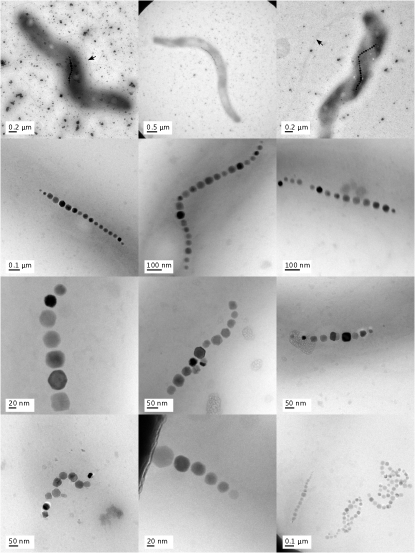
Figure 21: Transmission electron micrographs of MSR-1, magnetosomes and chains. The top row shows typical full scale bacteria, where black arrows indicate the flagella. Compared to the second row, the third row shows shorter chains with a higher variety in size distribution of magnetic nanoparticles due to an immaturity of the chain Uebe and Schüler (2016). The bottom row shows irregular chains and overlapping groups of expelled chains due to the formation of aggregates, making it hard or impossible to distinguish individual chains.

From these values the demagnetisation factor $\Delta N$, the magnetic moment $m$, and the maximum torque $\Gamma_{\text{max}}$ are calculated using the model from section II.1, and tabulated in table 2. Again, the standard deviations of the values and the 10%- and $90\text{\,}\mathrm{\char 37\relax}$ cut-off values are determined from Monte Carlo simulations.

Figure 22: Distance between magnetite particles as a function of the number of particles in the chain. The mean of the entire sample group is indicated with a dashed line at $56\pm 1.\text{\,}\mathrm{n}\mathrm{m}$. Vertical error bars represent the standard error of each individual chain.

IV.1.3 Average rate of rotation

From the drag coefficient $f_{\text{r}}$ and the maximum torque $\Gamma_{\text{max}}$, the ratio $\gamma$ between the average rate of rotation and the magnetic field strength can be obtained using equation 30. This value is listed as $\gamma_{\text{theory}}$ in table 2, and has a convenient value of approximately $1\text{\,}\mathrm{r}\mathrm{a}\mathrm{d}\mathrm{/}\mathrm{m}\mathrm{T}\mathrm{s}$. So in the earth’s magnetic field ($0.04\text{\,}\mathrm{m}\mathrm{T}$), the rate of rotation of an MSR-1 is approxmately $0.04\text{\,}\mathrm{r}\mathrm{a}\mathrm{d}\mathrm{/}\mathrm{s}$. A U-turn will take at least $78\text{\,}\mathrm{s}$.

IV.1.4 Average Velocity

The MTBs’ velocity was determined from the full set of 174 analyzed bacteria trajectories. This set has a mean velocity of $49.5\pm 0.7\text{\,}\mathrm{\SIUnitSymbolMicro}\mathrm{m}\mathrm{/}\mathrm{s}$ with a standard deviation $\sigma$ of $8.6\text{\,}\mathrm{\SIUnitSymbolMicro}\mathrm{m}\mathrm{/}\mathrm{s}$ (figure 23). Using the value for the average rate of rotation $\gamma$ of approximately $1\text{\,}\mathrm{r}\mathrm{a}\mathrm{d}\mathrm{/}\mathrm{m}\mathrm{T}\mathrm{s}$, this speed leads to a U-turn in the earth’s magnetic field of about $1\text{\,}\mathrm{m}\mathrm{m}$ (equation 30).

Comparing the velocity of Magnetospirillum Gryphiswaldensen in the vicinity of an oxic-anoxic zone (OAZ), $13\pm 1.\text{\,}\mathrm{\SIUnitSymbolMicro}\mathrm{m}\mathrm{/}\mathrm{s}$ to $23\pm 3.\text{\,}\mathrm{\SIUnitSymbolMicro}\mathrm{m}\mathrm{/}\mathrm{s}$ Lefèvre et al. (2014) (orientation towards OAZ-dependent), or without, $42\pm 4.\text{\,}\mathrm{\SIUnitSymbolMicro}\mathrm{m}\mathrm{/}\mathrm{s}$ Popp et al. (2014), suggests our value of the velocity of the MTB is not restricted by an oxygen gradient. Depending on the choice of binning, one might recognise a dip in the velocity distribution. Similar dips have been found in previous research, which were attributed to different swimming modes Reufer et al. (2014). There might as well be possible wall-effects on bacteria caused by the restricted space in the microfluidic chip Magariyama et al. (2005).

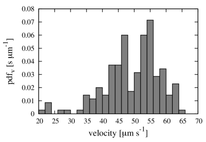
Figure 23: Probability density function for the MTB velocity distribution for $174$ observed MTB.

The measured velocity during U-turns as a function of the magnetic field strength is shown in figure 24. The vertical error bars display the standard error of the velocity within the group. The size of the sample group is depicted above the vertical error bars. For every sample group containing less than ten bacteria, the standard deviation of the entire population was used instead. The error in the magnetic field is due to positioning error, as described in section III.4.

On the scale of the graph, the deviation from the mean velocity is seemingly large, especially below $2\text{\,}\mathrm{m}\mathrm{T}$. This deviation is however not statistically significant. The reduced $\chi^{2}$ of the fit to the field-independent model is very close to unity ($0.67$), with a high $Q$-value of $0.77$ (the probability that $\chi^{2}$ would even exceed that value by chance, see Press et al., chapter 15 Press et al. (1992)). Within the standard errors obtained in this measurement, and for the range of field values applied, we can conclude that the velocity of the MTB is independent of the applied magnetic field, as expected.

Figure 24: Average MTB velocity as function of the applied magnetic field. The vertical error bars indicate the standard error calculated from the number of bacteria indicated above the error bar.

IV.2 Trajectories

The diameter $D$ of the U-turn was measured from the trajectories as in figure 16. From these values and the measured velocity $v$ for each individual bacterium, the average rate of rotation $v/D$ can be calculated. Figure 25 shows this average rate of rotation as a function of the applied magnetic field, $B$. The error bars are defined as in figure 24.

The data points are fitted to the U-turn trajectory model simulations of section II.2. The fit is shown as a solid black line, with the proportionality factor $\gamma_{\text{exp}}$ equal to $0.74\pm 0.03\text{\,}\mathrm{r}\mathrm{a}\mathrm{d}\mathrm{/}\mathrm{m}\mathrm{T}\mathrm{s}$. The reduced $\chi^{2}$ of the fit is ($2.88$), and the $Q$-value ($0.000\,86$)

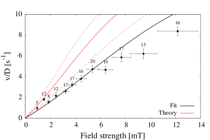
Figure 25: The average rate of rotation, $v/D$, as a function of the applied magnetic field, $B$. Vertical error bars display the standard error calculated for the number of MTB denoted above the error bars. For remaining sample groups, containing less than 10 bacteria samples, the standard deviation of the entire population is used instead. The black solid line is the fit of the model to the measured data, resulting in $\gamma_{\text{exp}}=$$0.74\pm 0.03\text{\,}\mathrm{r}\mathrm{a}\mathrm{d}\mathrm{/}\mathrm{m}\mathrm{T}\mathrm{s}$. The solid red line is the model prediction, using the $\gamma_{\text{theory}}$ derived from the bacteria and magnetosome dimensions, with the dotted red lines indicating the error on the estimate ($1.2\pm 0.3\text{\,}\mathrm{r}\mathrm{a}\mathrm{d}\mathrm{/}\mathrm{m}\mathrm{T}\mathrm{s}$).

Figure 25 shows that the observed average rate of rotation in low fields is higher than the model fit in comparison with the measurement error. We neglected the effect of the (earth’s) magnetic background field. As discussed before, at this field strength, however, the average rate of rotation is on the order of $40\text{\,}\mathrm{m}\mathrm{r}\mathrm{a}\mathrm{d}\mathrm{/}\mathrm{s}$ and the corresponding diameter of a U-turn is on the order of $1\text{\,}\mathrm{m}\mathrm{m}$. The background field can therefore not be the cause of any deviation at low field strengths. Tracking during the pre-processing step under low fields leads to an overlap between the trajectories, which affect the post-processing step. Due to the manual selection in the post-processing, illustrated in figure 16, the preference for uninterrupted and often shorter trajectories may have led (for lower fields) to a selection bias to smaller curvatures. The deviation from the linear fit below $2\text{\,}\mathrm{m}\mathrm{T}$ could therefore be attributed to human bias (“cherry picking”).

If we neglect trajectories below $2\text{\,}\mathrm{m}\mathrm{T}$ for this reason, the fits improve (drastically) for both the velocity and average rate of rotation. Fitting datapoints over the range of $212\text{\,}\mathrm{m}$T (eight degrees of freedom) decreases the reduced $\chi^{2}$ of the velocity from $0.67$ to $0.42$. Furthermore, the $Q$-value of $0.77$ is increased to $0.91$, a slight increase in likelihood that our datapoints fall within the limits of the model.

Similarly, the reduced $\chi^{2}$ of the average rate of rotation is lowered from $2.88$ to $1.03$ and the $Q$-value from $0.000\,86$ to $0.41$, a drastic change in likelihood of the fit. We therefore assume that these results validate the model with the exclusion of outliers below $2\text{\,}\mathrm{m}\mathrm{T}$.

At high fields, the observed average rate of rotation seems to be on the low side, although within the error bounds. For the high field range, the diameter of a U-turn is on the order of $5\text{\,}\mathrm{\SIUnitSymbolMicro m}$ and reversal times are on the order of $100\text{\,}\mathrm{m}\mathrm{s}$. The resolving power of our setup of $180\text{\,}\mathrm{n}\mathrm{m}\mathrm{/}\mathrm{p}\mathrm{i}\mathrm{x}\mathrm{e}\mathrm{l}$ and time resolution of $100\text{\,}\mathrm{f}\mathrm{r}\mathrm{a}\mathrm{m}\mathrm{e}\mathrm{s}\mathrm{/}\mathrm{s}$ are sufficient to capture these events, so cannot explain the apparent deviation. It is possible that the weakest bacteria reach the saturation torque (figure 4), although the effect is not expected to be very significant.

V Discussion

Figure 25 shows in red the prediction of the model using the proportionality factor determined from observations of the MTB (the outer dimensions by optical microsopy and SEM, the magnetosome by TEM), $\gamma_{\text{theory}}$=$1.2\pm 0.3\text{\,}\mathrm{r}\mathrm{a}\mathrm{d}\mathrm{/}\mathrm{m}\mathrm{T}\mathrm{s}$. The predicted proportionaliy factor is clearly higher than measured. This is either because we overestimated the magnetic moment or underestimated the rotational drag coeffient. The latter seems more likely. In the the first place, we neglected the influence of the flagella. A coarse estimate using a rigid cylinder model for the flagellum shows that a flagellum could indeed cause this type of increase in drag. Since we lack information on the flexibility of the flagellum, we cannot quantify the additional drag. Secondly, we ignored the finite height of the microfluidic channel. As was shown by the macroscale experiments, the additional drag increases rapidly if a bacterium approaches within a few hundred nanometers of the wall. Since we do not have information about the distance, again quantification is difficult.

Given the above considerations, we are confident that over the observed field range, the MTB trajectories are in fair agreement with our model.

VI Conclusion

We studied the response of the magnetotactic bacteria Magnetospirillum Gryphiswaldense to rotation of an external magnetic field $B$, ranging in amplitude from $1\text{\,}\mathrm{m}\mathrm{T}$ up to $12\text{\,}\mathrm{m}\mathrm{T}$.

Our magnetic model shows that the torque on the MTB is linear in the applied field up to $10\text{\,}\mathrm{m}\mathrm{T}$, after which the torque starts to saturate for an increasing part of the population.

Our theoretical analysis of bacterial trajectories shows that the bacteria perform a U-turn under $180\text{\,}\mathrm{\SIUnitSymbolDegree}$ rotation of the external field, but not at a constant angular velocity. The diameter, $D$, of the U-turn increases with an increase in the velocity $v$ of the bacteria. The average rate of rotation, $v/D$, for an instantaneously reversing field is linear within $2\text{\,}\%$ in the applied field up to $12\text{\,}\mathrm{m}\mathrm{T}$.

If the applied field is rotated over $180\text{\,}\mathrm{\SIUnitSymbolDegree}$ in a finite time, the average rate of rotation is higher at low field values than it was for an instantaneous reversal. Given a field rotation time, an optimum field value exist at which the rate of rotation is approximately $18\text{\,}\mathrm{\char 37\relax}$ higher than for instantaneous reversal. This optimum field value is inversely proportional to the field rotation time.

The rotational drag coefficient for an MTB was estimated from drag rotation experiments in a highly viscous fluid, using a macroscale 3D printed MTB model. The spiral shape of the body of an MTB has a $64\pm 5.\text{\,}\mathrm{\char 37\relax}$ higher drag than a spheroid with equal length and diameter, which has been the default model in the literature up to now. Furthermore, the added drag from the channel wall was found to be negligible for an MTB in the center between the walls (less than $10\text{\,}\mathrm{\char 37\relax}$), but to increase rapidly when the MTB approaches to within a few hundred nanometers of one of the walls.

From microscope observations, we conclude that the MTB velocity during a U-turn is independent of the applied field. The population of MTB has a non-Gaussian distributed velocity, with an average of $49.5\pm 0.7\text{\,}\mathrm{\SIUnitSymbolMicro}\mathrm{m}\mathrm{/}\mathrm{s}$ and a standard deviation of $8.6\text{\,}\mathrm{\SIUnitSymbolMicro}\mathrm{m}\mathrm{/}\mathrm{s}$. As predicted by our model, the average rate of rotation is linear in the external magnetic field within the measured range of $112\text{\,}\mathrm{m}\mathrm{T}$. The proportionality factor $\gamma=v/DB$ equals $0.74\pm 0.03\text{\,}\mathrm{r}\mathrm{a}\mathrm{d}\mathrm{/}\mathrm{m}\mathrm{T}\mathrm{s}$. The predicted theoretical value is $1.2\pm 0.3\text{\,}\mathrm{r}\mathrm{a}\mathrm{d}\mathrm{/}\mathrm{m}\mathrm{T}\mathrm{s}$, which is based on measurements of the parameters needed for the model, such as the size of the bacteria and their magnetosomes from optical microscopy, SEM, and TEM images. The number of parameters and their nonlinear relation with the proportionality factor causes the relatively large error in the estimate.

These findings finally prove that the generally accepted linear model for the response of MTB to external magnetic fields is correct within the errors caused by the estimation of the model parameters if the field values are below $12\text{\,}\mathrm{m}\mathrm{T}$. At higher values, torque saturation will occur.

This result is of importance to the control engineering community. The knowledge of the relation between the angular velocity and the field strength ($\gamma$) can be used to design energy efficient control algorithms that prevent the use of excessive field strengths. Furthermore, a better understanding of the magnetic behavior will lead to more accurate predictions of the dynamic response of MTB for potential applications in micro-surgery, as drug carriers, or for drug delivery.