Efficient Preconditioning for Noisy Separable NMFs by Successive Projection Based Low-Rank Approximations

Abstract

The successive projection algorithm (SPA) can quickly solve a nonnegative matrix factorization problem under a separability assumption. Even if noise is added to the problem, SPA is robust as long as the perturbations caused by the noise are small. In particular, robustness against noise should be high when handling the problems arising from real applications. The preconditioner proposed by Gillis and Vavasis (2015) makes it possible to enhance the noise robustness of SPA. Meanwhile, an additional computational cost is required. The construction of the preconditioner contains a step to compute the top-$k$ truncated singular value decomposition of an input matrix. It is known that the decomposition provides the best rank-$k$ approximation to the input matrix; in other words, a matrix with the smallest approximation error among all matrices of rank less than $k$. This step is an obstacle to an efficient implementation of the preconditioned SPA.

To address the cost issue, we propose a modification of the algorithm for constructing the preconditioner. Although the original algorithm uses the best rank-$k$ approximation, instead of it, our modification uses an alternative. Ideally, this alternative should have high approximation accuracy and low computational cost. To ensure this, our modification employs a rank-$k$ approximation produced by an SPA based algorithm. We analyze the accuracy of the approximation and evaluate the computational cost of the algorithm. We then present an empirical study revealing the actual performance of the SPA based rank-$k$ approximation algorithm and the modified preconditioned SPA.

Keywords: separable nonnegative matrix factorization, robustness, successive projection, singular value decomposition, low-rank approximation, hyperspectral unmixing

1 Introduction

Given $\bm{M}\in\mathbb{R}^{d\times m}_{+}$ and a positive integer $k$, a nonnegative matrix factorization (NMF) problem is one of finding $\bm{F}\in\mathbb{R}^{d\times k}_{+}$ and $\bm{W}\in\mathbb{R}^{k\times m}_{+}$ such that $\|\bm{F}\bm{W}-\bm{M}\|_{F}$ is minimized. Here, a nonnegative matrix is a real matrix whose elements are all nonnegative, and $\mathbb{R}^{d\times m}_{+}$ denotes the set of $d\times m$ nonnegative matrices. Although NMF problems cover a broad range of applications, they are often intractable. Indeed, the NMF problem was shown to be NP-hard in [35]; also see [4] for a further discussion on the hardness of the problem. However, the situation changes if we make the separability assumption, introduced in [12, 4, 5].

Let $\bm{M}\in\mathbb{R}^{d\times m}_{+}$ have an exact NMF such that $\bm{M}=\bm{F}\bm{W}$ for $\bm{F}\in\mathbb{R}^{d\times k}_{+}$ and $\bm{W}\in\mathbb{R}^{k\times m}_{+}$. Separability assumes that $\bm{M}$ can be further written as

$$\bm{M}=\bm{F}\bm{W}\ \mbox{for}\ \bm{F}\in\mathbb{R}^{d\times k}_{+}\ \mbox{and}\ \bm{W}=[\bm{I},\bm{H}]\bm{\Pi}\in\mathbb{R}^{k\times m}_{+}.$$ (1)

Here, $\bm{I}$ is the $k\times k$ identity, $\bm{H}$ is a $k\times(m-k)$ nonnegative matrix, and $\bm{\Pi}$ is an $m\times m$ permutation matrix. We call $\bm{F}$ the basis of $\bm{M}$ and $k$ the factorization rank. If a nonnegative matrix $\bm{M}$ can be written as (1), we call it a separable matrix. The feature of separable matrices is that all columns of $\bm{F}$ appear in those of $\bm{M}$. The separable NMF problem is stated as follows.

Problem 1.

Let $\bm{M}$ be of the form given as (1). Find a column index set $\mathcal{I}$ with $k$ elements such that $\bm{M}(\mathcal{I})$ coincides with the basis $\bm{F}$.

The notation $\bm{M}(\mathcal{I})$ denotes the submatrix of $\bm{M}$ indexed by $\mathcal{I}$; in other words, $\bm{M}(\mathcal{I})=[\bm{m}_{i}:i\in\mathcal{I}]$ for the $i$th column $\bm{m}_{i}$ of $\bm{M}$. The problem is solvable in polynomial time [4].

Separable matrices arise in applications, such as endmember detection in hyperspectral images [28, 6, 23, 15, 16, 14] and topic extraction from documents [4, 5, 3, 26]. In such applications, it should be reasonable to assume that separability is affected by noise. Noisy separability assumes that a separable matrix $\bm{M}$ given as (1) is perturbed by $\bm{N}\in\mathbb{R}^{d\times m}$. That is,

$$\bm{A}=\bm{M}+\bm{N}=\bm{F}\bm{W}+\bm{N}\ \mbox{for}\ \bm{F}\in\mathbb{R}^{d\times k}_{+},\bm{W}=[\bm{I},\bm{H}]\bm{\Pi}\in\mathbb{R}^{k\times m}_{+}\ \mbox{and}\ \bm{N}\in\mathbb{R}^{d\times m}.$$

If a nonnegative matrix $\bm{A}$ can be written as above, we call it a noisy separable matrix. Consider an algorithm for solving separable NMF problems. Given a noisy separable matrix $\bm{A}$ and factorization rank $k$, we say that the algorithm is robust to noise if it can find a column index set $\mathcal{I}$ with $k$ elements such that $\bm{A}(\mathcal{I})$ is close to the basis $\bm{F}$ of $\bm{A}$.

The successive projection algorithm (SPA) was originally proposed by [2] in the context of chemometrics. Recently, Gillis and Vavasis showed in [15] that SPA works well at solving separable NMF problems. Given a separable matrix $\bm{M}$ and a factorization rank $k$ as input, SPA finds a column index set $\mathcal{I}$ with $k$ elements such that $\bm{M}(\mathcal{I})$ coincides with the basis $\bm{F}$. Even if noise is involved, it is robust to small perturbations caused by it. The results in [15] imply that the robustness of SPA can be further improved if one can make the condition number of the basis in a noisy separable matrix smaller. Accordingly, Gillis and Vavasis proposed the preconditioned SPA (PSPA) in [16]. The results in [16, 27] imply that PSPA is more robust than SPA.

Although PSPA is more robust than SPA, it has an issue in regard to its computational cost. To see this clearly, let us recall how PSPA constructs a conditioning matrix. The input is $\bm{A}\in\mathbb{R}^{d\times m}$ and a positive integer $k$. The construction of the conditioning matrix consists of two steps. The first step computes the top-$k$ truncated singular value decomposition (SVD) $\bm{A}_{k}=\bm{U}_{k}\bm{\Sigma}_{k}\bm{V}_{k}^{\top}$ of $\bm{A}$ and then constructs $\bm{P}=\bm{\Sigma}_{k}\bm{V}_{k}^{\top}\in\mathbb{R}^{k\times m}$. We will explain the decomposition in Section 2.2, and $\bm{U}_{k},\bm{V}_{k}$ and $\bm{\Sigma}_{k}$ are of the form specified in (3) and (2). The second step computes a $k\times k$ positive definite matrix $\bm{L}^{*}$ such that $\{\bm{x}\in\mathbb{R}^{k}:\bm{x}^{\top}\bm{L}^{*}\bm{x}\leq 1\}$ is a minimum-volume enclosing ellipsoid for the set of columns $\bm{p}_{1},\ldots,\bm{p}_{m}$ of $\bm{P}$. This can be obtained by solving a convex optimization problem. Since $\bm{L}^{*}$ is positive definite, there is a $\bm{C}\in\mathbb{R}^{k\times k}$ such that $\bm{L}^{*}=\bm{C}^{2}$. PSPA forms $\bm{P}^{\circ}=\bm{C}\bm{P}$ and runs SPA for $\bm{P}^{\circ}$.

PSPA needs to compute a truncated SVD in the first step and solve a convex optimization problem in the second step. In practice, the computational cost of solving the optimization problem can be sufficiently reduced by employing a cutting plane strategy. Experimental evidence for this was presented in previous studies [31, 1]. A truncated SVD can be computed in polynomial time. Given a $d\times m$ matrix with $d\leq m$, the truncated SVD can be obtained by constructing the full SVD and then truncating it. This approach takes $O(d^{2}m)$. However, the computation of a truncated SVD is challenging when the matrix is large. In such cases, the first step is an obstacle to an efficient implementation of PSPA.

1.1 Our Algorithms and Contributions

The aim of this paper is to develop a modification of PSPA such that its robustness against noise is high and its computational cost is low. We modify the first step of PSPA. The step computes the top-$k$ truncated SVD $\bm{A}_{k}=\bm{U}_{k}\bm{\Sigma}_{k}\bm{V}_{k}^{\top}$ of an input matrix $\bm{A}$. Regarding $\bm{A}_{k}$, the Eckart-Young-Mirsky theorem tells us that

$$\min_{\scriptsize\mbox{rank}(\bm{B})\leq k}\|\bm{A}-\bm{B}\|=\|\bm{A}-\bm{A}_{k}\|$$

holds when the norm is the $L_{2}$ norm or the Frobenius norm. A matrix is called a rank-$k$ approximation to $\bm{A}$ if it is the same size as $\bm{A}$ and is at most rank $k$. We can see from the theorem that $\bm{A}_{k}$ is the best rank-$k$ approximation to $\bm{A}$ under the norms. Although PSPA uses $\bm{A}_{k}$, our modification replaces it with an alternative rank-$k$ approximation.

The key to the development of our modified PSPA is the method for constructing a rank-$k$ approximation to a matrix. Ideally, the approximation accuracy should be high and the computational cost should be low. If the accuracy of the rank-$k$ approximation is close enough to that of the best approximation, the modified PSPA is expected to be as robust to noise as PSPA. We incorporate an SPA based rank-$k$ approximation in the modified PSPA. Algorithm 1 describes each step of the algorithm. $\mathcal{I}$ of Step 1 is a subset of $\{1,\ldots,m\}$ with $k$ elements (Algorithm 2 shows the details of SPA). Since the rank of $\bm{Q}$ is less than or equal to $k$, the output matrix $\bm{B}$ serves as a rank-$k$ approximation to $\bm{A}$. The modified PSPA forms $\bm{P}=\bm{Q}^{\top}\bm{A}$ by using $\bm{Q}$ at Step 3 of Algorithm 1; then, it constructs a minimum-volume enclosing ellipsoid for the columns of $\bm{P}$.

Algorithm 1 SPA based rank-$k$ approximation

Input: $\bm{A}\in\mathbb{R}^{d\times m}$ and integers $q$ and $k$ such that $0\leq q$ and $0<k\leq\min\{d,m\}$
Output: $\bm{B}\in\mathbb{R}^{d\times m}$

1. Run SPA on the input $(\bm{A},k)$ and let $\mathcal{I}$ be the output.

2. Form $\bm{Y}=(\bm{A}\bm{A}^{\top})^{q}\bm{A}(\mathcal{I})\in\mathbb{R}^{d\times k}$.

3. Compute the orthonormal bases of the range space of $\bm{Y}$ and form a matrix $\bm{Q}$ by stacking them in a column.

4. Form $\bm{B}=\bm{Q}\bm{Q}^{\top}\bm{A}$ and return it.

Algorithm 1 has a close relationship with a randomized algorithm in a subspace iteration framework [30, 20, 37, 18]. The randomized algorithm is sometimes referred to as the randomized subspace iteration. In contrast to $\bm{Y}$ in Step 2, the randomized algorithm forms $\bm{Y}=(\bm{A}\bm{A}^{\top})^{q}\bm{A}\bm{\Omega}$ using a Gaussian matrix $\bm{\Omega}$. We will see the relationship between the algorithms in Section 5.3. It should be noted that Algorithm 1 is deterministic, while the randomized algorithm is probabilistic, as it exploits the randomness of a Gaussian matrix.

Our first contribution is to provide a theoretical assessment of Algorithm 1. We derive a bound on the error $\|\bm{A}-\bm{B}\|_{2}$ for the input matrix $\bm{A}$ and output matrix $\bm{B}$. The main result is Theorem 3. The theorem tells us that, if $\bm{A}$ is noisy separable and the amount of noise is smaller than certain level, then, the error is close to the best error and decreases toward the best error as $q$ increases. We show in Section 5.1 that the algorithm takes $O(dmkq)$ arithmetic operations on $\bm{A}\in\mathbb{R}^{d\times m}$ and integers $q$ and $k$.

Our second contribution is a modification of PSPA that uses Algorithm 1. The importance of data preprocessing in SPA has been recognized, and there are several studies [28, 26, 14, 32] on it. Among them, Gillis and Ma proposed a modification of PSPA in [14]. It aimed to resolve the cost issue of PSPA. The basic idea is to skip the computation of an enclosing ellipsoid and only perform the computation of a truncated SVD. Hence, our modification differs from their modification. One of the favorable features of our modification is that its robustness against noise increases with $q$.

Our third contribution is an experimental assessment of Algorithm 1 and the modified PSPA. The results are summarized as follows.

• Experiments were conducted on synthetically generated noisy separable matrices. When $q$ exceeds $10$, the error of Algorithm 1 was close to the best error, and the modified PSPA significantly improved the robustness to noise compared with SPA, even if the amount of noise was large. Algorithm 1 with $q=10$ often provided highly accurate low-rank approximations, and the elapsed time was much shorter than that of a truncated SVD computation. These results are displayed in Figures 1 and 2 and in Table 2.

• We applied the modified PSPA to a hyperspectral unmixing problem. Experiments were conducted on the HYDICE urban data. When $q=4$, the estimation of endmembers by the modified PSPA coincided with that by PSPA. The estimation was close to the spectra of constituent materials identified in the previous study [38]. The experimental results suggested the possibility that for hyperspectral unmixing, the modified PSPA provides the similar results to those of PSPA in less computational time. These results are shown in Table 5 and Figure 4.

The rest of this paper is organized as follows. Section 2 describes the notation and definitions that are necessary for our discussion. In addition, it reviews SVD and low-rank approximations to matrices. Section 3 overviews SPA and PSPA and discusses the computational cost of PSPA. Section 4 presents the modified PSPA and describes the results of our analysis on Algorithm 1. The details of the analysis are given in Section 5. This section also overviews the randomized subspace iteration. Section 6 reports an empirical study on synthetic and real data. Section 7 gives a summary and suggests future research directions.

2 Preliminaries

2.1 Notation and Definitions

Let $\mathbb{R}$ denotes the set of real numbers, and $\mathbb{R}^{d\times m}$ the set of $d\times m$ real matrices. We use a capital upper-case letter $\bm{A}$ to denote a matrix. A capital lower-case letter with subscript $\bm{a}_{i}$ indicates the $i$th column, and a lower-case letter with subscript $a_{ij}$ indicates the $(i,j)$th element. Let $\bm{A}\in\mathbb{R}^{d\times m}$. We denote by $\bm{A}^{\top}$ and $\mbox{rank}(\bm{A})$ the transpose and rank of $\bm{A}$. The notation $\|\bm{A}\|$ stands for the norm of $\bm{A}$; in particular, $\|\bm{A}\|_{2}$ and $\|\bm{A}\|_{F}$ indicate the $L_{2}$ norm and Frobenius norm. If the matrix size needs to be specified, we use the notation $\bm{A}_{d\times m}$ to mean that $\bm{A}$ is $d\times m$.

Let us suppose that $\bm{A}$ is $d\times m$. We say that it is diagonal if $a_{ij}=0$ for every $i\neq j$. The element $a_{ii}$ of a diagonal matrix $\bm{A}$ is abbreviated as $a_{i}$. Let us recall the definition of positive definite and positive semidefinite matrices. Suppose that $\bm{A}$ is symmetric. It is positive semidefinite if $\bm{x}^{\top}\bm{A}\bm{x}\geq 0$ for every $\bm{x}\neq\bm{0}$, and, in particular, it is positive definite if the inequality holds strictly. It is known that $\bm{A}$ is positive semidefinite (resp. positive definite) if and only if all the eigenvalues of $\bm{A}$ are nonnegative (resp. positive). Thus, a positive definite matrix is nonsingular.

The notations $\bm{I}$, $\bm{0}$, $\bm{\Pi}$, $\bm{e}$ and $\bm{e}_{i}$ are used to denote the following matrices and vectors; $\bm{I}$ is the identity matrix; $\bm{0}$ is the all-zero matrix; $\bm{\Pi}$ is a permutation matrix; $\bm{e}$ is the vector of all ones; and $\bm{e}_{i}$ is the $i$th unit vector.

2.2 SVD and Low-Rank Approximations

Let $\bm{A}\in\mathbb{R}^{d\times m}$. It can be factorized into

$$\bm{A}=\bm{U}\bm{\Sigma}\bm{V}^{\top}.$$

Here, $\bm{U}$ and $\bm{V}$ are $d\times d$ and $m\times m$ orthogonal matrices, and $\bm{\Sigma}$ is a $d\times m$ diagonal matrix with nonnegative diagonal elements $\sigma_{1}\geq\cdots\geq\sigma_{t}\geq 0$ where $t=\min\{d,m\}$. This factorization is called the singular value decomposition and it is commonly abbreviated by SVD. The diagonal elements $\sigma_{1},\ldots,\sigma_{t}$ are called the singular values. Obviously, the number of positive singular values coincides with the rank. We denote by $\sigma_{\mbox{\scriptsize max}}$ and $\sigma_{\mbox{\scriptsize min}}$ the largest and smallest singular values. Throughout this paper, we use $\sigma_{i}$ to denote the $i$th largest singular value of $\bm{A}$. When referring to singular values of several different matrices $\bm{A}$ and $\bm{B}$, and so on, to prevent confusion, the notation $\sigma_{i}(\bm{A})$ is used to denote the $i$th largest singular value of $\bm{A}$. We define the condition number of $\bm{A}$ as $\sigma_{\mbox{\scriptsize max}}(\bm{A})/\sigma_{\mbox{\scriptsize min}}(\bm{A})$, and denote it by $\kappa(\bm{A})$.

By picking the top $k$ singular values $\sigma_{1},\ldots,\sigma_{k}$ in $\bm{\Sigma}$, we form a $k\times k$ diagonal matrix,

$$\bm{\Sigma}_{k}=\left[\begin{array}[]{ccc}\sigma_{1}&&\\ &\ddots&\\ &&\sigma_{k}\\ \end{array}\right]\in\mathbb{R}^{k\times k}$$ (2)

and also form

$$\bm{U}_{k}=[\bm{u}_{1},\ldots,\bm{u}_{k}]\in\mathbb{R}^{d\times k}\ \mbox{and}\ \bm{V}_{k}=[\bm{v}_{1},\ldots,\bm{v}_{k}]\in\mathbb{R}^{m\times k}$$ (3)

for the first $k$ columns $\bm{u}_{1},\ldots,\bm{u}_{k}$ in $\bm{U}$ and those $\bm{v}_{1},\ldots,\bm{v}_{k}$ in $\bm{V}$. Let

$$\bm{A}_{k}=\bm{U}_{k}\bm{\Sigma}_{k}\bm{V}_{k}^{\top}.$$

We call it the top-$k$ truncated SVD of $\bm{A}$. Suppose that $k$ is a positive integer such that $k<\mbox{rank}(\bm{A})$. Then,

$$\min_{\scriptsize\mbox{rank}(\bm{B})\leq k}\|\bm{A}-\bm{B}\|_{2}=\|\bm{A}-\bm{A}_{k}\|_{2}=\sigma_{k+1},$$

$$\min_{\scriptsize\mbox{rank}(\bm{B})\leq k}\|\bm{A}-\bm{B}\|_{F}=\|\bm{A}-\bm{A}_{k}\|_{F}=\sqrt{\sigma_{k+1}^{2}+\cdots+\sigma_{t}^{2}},$$

where $t=\min\{d,m\}$. This result is known as the Eckart-Young-Mirsky theorem; see [13, 34, 17] for the details. We can see that $\bm{A}_{k}$ is the best rank-$k$ approximation to $\bm{A}$ under the $L_{2}$ norm error or Frobenius norm error.

In the subsequent discussion, we will use two well-known results on singular values. The first one is about singular value perturbations, and the second one is called the interlacing property.

Lemma 1 (Corollary 8.6.2 of [17]).

Let $\bm{A}\in\mathbb{R}^{d\times m}$ and $\bm{N}\in\mathbb{R}^{d\times m}$. Then, $|\sigma_{i}(\bm{A}+\bm{N})-\sigma_{i}(\bm{A})|\leq\|\bm{N}\|_{2}$ holds for $i=1,\ldots,t$, where $t=\min\{d,m\}$.

Lemma 2 (Theorem 8.1.7 and Corollary 8.6.3 in [17]).

Let $\bm{A}\in\mathbb{R}^{d\times m}$. Suppose that $k$ is an integer such that $0<k\leq\min\{d,m\}$. Let $\bm{B}$ be the $d\times k$ submatrix of $\bm{A}$ consisting of the first $k$ columns. Then, $\sigma_{k}(\bm{A})\geq\sigma_{k}(\bm{B})$ or equivalently $\sigma_{\mbox{\scriptsize min}}(\bm{B})$ holds.

In Lemma 2, let $\bm{C}$ be the $k\times k$ submatrix of $\bm{A}$ consisting of the first $k$ rows and first $k$ columns. Then, the lemma implies $\sigma_{k}(\bm{A})\geq\sigma_{k}(\bm{B})=\sigma_{k}(\bm{B}^{\top})\geq\sigma_{k}(\bm{C}^{\top})=\sigma_{k}(\bm{C})$, since $\bm{C}^{\top}$ is the submatrix of $\bm{B}^{\top}$ consisting of the first $k$ columns.

3 SPA and PSPA

3.1 SPA

Let us observe a separable matrix from a geometrical point of view. Let $\bm{M}=\bm{F}\bm{W}$ for $\bm{F}\in\mathbb{R}^{d\times k}_{+}$ and $\bm{W}=[\bm{I},\bm{H}]\bm{\Pi}\in\mathbb{R}^{k\times m}_{+}$. As discussed in [4], without loss of generality, every column $\bm{h}_{i}$ of $\bm{H}$ can be assumed to satisfy $\bm{e}^{\top}\bm{h}_{i}=1$. In addition, we assume that $\mbox{rank}(\bm{F})=k$. This assumption may be reasonable from the standpoint of a practical application, because, in such cases, it is less common for the columns of $\bm{F}$ to be linearly dependent. Thus, the convex hull of the columns of $\bm{M}$ is a $(k-1)$-dimensional simplex in $\mathbb{R}^{d}$, and the vertices correspond to the columns of $\bm{F}$. Accordingly, a separable NMF problem without noise can be restated as follows. Let $\mathcal{S}$ be the set of points, including all vertices, in a $(k-1)$-dimensional simplex in $\mathbb{R}^{d}$. Find all points corresponding to the vertices of the simplex from $\mathcal{S}$. SPA finds a correct answer for a problem by exploiting the property that the maximum of a strongly convex function over the set $\mathcal{S}$ is attained at one of the vertices. It uses $f(\bm{x})=\|\bm{x}\|_{2}^{2}$ and chooses a point to maximize $f$ over $\mathcal{S}$. Then, it projects all points of $\mathcal{S}$ onto the orthogonal space to the chosen point. Algorithm 2 describes each step of SPA.

Algorithm 2 SPA [2, 15]

Input: $\bm{A}\in\mathbb{R}^{d\times m}$ and an integer $k$ such that $0<k\leq m$
Output: An index set $\mathcal{I}$

1. Initialize $\bm{S}\leftarrow\bm{A}$ and $\mathcal{I}\leftarrow\emptyset$.

2. Find $i^{*}=\arg\max_{i=1,\ldots,m}\|\bm{s}_{i}\|_{2}^{2}$ for the columns $\bm{s}_{1},\ldots,\bm{s}_{m}$ of $\bm{S}$.

3. Set $\bm{t}\leftarrow\bm{s}_{i^{*}}$. Update

   $$\bm{S}\leftarrow\biggl{(}\bm{I}-\frac{\bm{t}\bm{t}^{\top}}{\|\bm{t}\|_{2}^{2}}\biggr{)}\bm{S}\ \mbox{and}\ \mathcal{I}\leftarrow\mathcal{I}\cup\{i^{*}\},$$

4. If $|\mathcal{I}|<k$, go back to Step 2; otherwise, return $\mathcal{I}$ and terminate.

Now let us describe the results of Gillis and Vavasis [15] that SPA works well for solving separable NMF problems. Let $\bm{M}\in\mathbb{R}^{d\times m}$, and put the following assumption on it.

Assumption 1.

$\bm{M}$ can be written as

$$\bm{M}=\bm{F}\bm{W}\ \mbox{for}\ \bm{F}\in\mathbb{R}^{d\times k}\ \mbox{and}\ \bm{W}=[\bm{I},\bm{H}]\bm{\Pi}\in\mathbb{R}^{k\times m}_{+}.$$

Furthermore, $\bm{F}$ and the columns $\bm{h}_{i}$ of $\bm{H}$ satisfy

1. $\mbox{rank}(\bm{F})=k$.

2. $\bm{e}^{\top}\bm{h}_{i}\leq 1$ for $i=1,\ldots,m-k$.

$\bm{W}$ of Assumption 1 is the same as that of the separability assumption, whose description is given in (1). Meanwhile, $\bm{F}$ is more general than that of separability, since it does not have to be nonnegative. Gillis and Vavasis [15] showed that SPA for $\bm{M}$ satisfying Assumption 1 returns $\mathcal{I}$ such that $\bm{M}(\mathcal{I})$ coincides with $\bm{F}$ of $\bm{M}$. In addition, they showed that it is robust to noise.

Theorem 1 (Theorem 3 of [15]).

Let $\bm{A}=\bm{M}+\bm{N}$ for $\bm{M}\in\mathbb{R}^{d\times m}$ and $\bm{N}\in\mathbb{R}^{d\times m}$. Suppose that $k\geq 2$, $\bm{M}$ satisfies Assumption 1, and the columns $\bm{n}_{i}$ of $\bm{N}$ satisfy $\|\bm{n}_{i}\|_{2}\leq\epsilon$ for $i=1,\ldots,m$ with

$$\epsilon<\min\Biggl{\{}\frac{1}{2\sqrt{k-1}},\frac{1}{4}\Biggr{\}}\frac{\sigma_{\mbox{\scriptsize min}}(\bm{F})}{80\kappa(\bm{F})^{2}+1}.$$

Let $\mathcal{I}$ be the output of Algorithm 2 and $i_{1},\ldots,i_{k}$ be the elements in $\mathcal{I}$. Then, there is a permutation $\pi:\{1,\ldots,k\}\rightarrow\{1,\ldots,k\}$ such that

$$\|\bm{a}_{i_{j}}-\bm{f}_{\pi(j)}\|_{2}\leq(80\kappa(\bm{F})^{2}+1)\epsilon$$

for $j=1,\ldots,k$.

Although the description of Theorem 1 does not completely match that of Theorem 3 in [15], Theorem 1 almost directly follows from Theorem 3 of [15]. For the details, we refer readers to Remark 1 of [27] and Remark 1 of [16]. Theorem 1 tells us that SPA can extract the submatrix of a noisy separable matrix close to the basis if the amount of noise is small.

In addition to the results mentioned above, Gillis and Vavasis examined the computational cost of SPA. Step 3 of Algorithm 2 needs to compute the matrix multiplication of a $d\times d$ matrix $\bm{t}\bm{t}^{\top}/\|\bm{t}\|_{2}^{2}$ and a $d\times m$ matrix $\bm{S}$ for every iteration. The matrix multiplication requires in total $O(d^{2}mk)$ arithmetic operations. However, we can reduce these operations by taking into account the equality,

$$\|(\bm{I}-\bm{b}\bm{b}^{\top})\bm{a}\|_{2}^{2}=\|\bm{a}\|_{2}^{2}-(\bm{a}^{\top}\bm{b})^{2}\ \mbox{for}\ \bm{a}\in\mathbb{R}^{d}\ \mbox{and}\ \bm{b}\in\mathbb{R}^{d}\ \mbox{with}\ \|\bm{b}\|_{2}=1.$$ (4)

This allows SPA to run in $O(dmk)$ (see Remark 5 of [15]).

As pointed out in [11, 15], SPA is essentially the same as the QR factorization with column pivoting in [9]. The authors of [11] used SPA in the context of studying the complexity of the following problems. Given $\bm{A}\in\mathbb{R}^{d\times m}$ and a positive integer $k$, find the set $\mathcal{I}$ of $k$ column indices among all candidates to satisfy some criterion. The authors gave four criteria, including the following two: (a) $\sigma_{\mbox{\scriptsize min}}(\bm{A}(\mathcal{I}))$ is maximized, and (b) the volume of parallelepiped spanned by the columns of $\bm{A}(\mathcal{I})$ is maximized. They showed the NP-hardness of the problems. They also used SPA as a heuristic for solving the volume maximization problem and studied the accuracy of the heuristic.

3.2 PSPA

The use of a preconditioning matrix makes it possible to improve the robustness performance of SPA. Theorem 1 suggests that, if the condition number of $\bm{F}$ can be made close to one, the allowed noise magnitude range $\|\bm{n}_{i}\|_{2}$ increases and the basis gap $\|\bm{a}_{i_{j}}-\bm{f}_{\pi(j)}\|_{2}$ decreases. For $\bm{A}=\bm{F}\bm{W}+\bm{N}\in\mathbb{R}^{d\times m}$, we choose some matrix $\bm{C}\in\mathbb{R}^{d\times d}$ and apply it to $\bm{A}$ so that $\bm{C}\bm{A}=\bm{C}\bm{F}\bm{W}+\bm{C}\bm{N}$. If $\bm{C}$ is chosen to make the condition number of $\bm{C}\bm{F}$ small, the robustness of SPA might be improved by performing it on $\bm{C}\bm{A}$ instead of $\bm{A}$, although the amount of noise could be enlarged by up to a factor $\|\bm{C}\|_{2}$ because $\|\bm{C}\bm{N}\|_{2}\leq\|\bm{C}\|_{2}\|\bm{N}\|_{2}$. On the basis of this observation, in [16], Gillis and Vavasis proposed PSPA (Algorithm 3).

Algorithm 3 PSPA [16]

Input: $\bm{A}\in\mathbb{R}^{d\times m}$ and an integer $k$ such that $0<k\leq\min\{d,m\}$
Output: An index set $\mathcal{I}$

1. Compute the top-$k$ truncated SVD $\bm{A}_{k}=\bm{U}_{k}\bm{\Sigma}_{k}\bm{V}_{k}^{\top}$ of $\bm{A}$ and form $\bm{P}=\bm{\Sigma}_{k}\bm{V}_{k}^{\top}\in\mathbb{R}^{k\times m}$.

2. Let $\mathcal{S}=\{\bm{p}_{1},\ldots,\bm{p}_{m}\}$ for the columns $\bm{p}_{1},\ldots,\bm{p}_{m}$ of $\bm{P}$ and compute the optimal solution $\bm{L}^{*}$, which is a $k\times k$ positive definite matrix, of the optimization problem $\mathrm{P}(\mathcal{S})$.

3. Compute $\bm{C}\in\mathbb{R}^{k\times k}$ such that $\bm{L}^{*}=\bm{C}^{2}$ and form $\bm{P}^{\circ}=\bm{C}\bm{P}$.

4. Run Algorithm 2 on input $(\bm{P}^{\circ},k)$ and return the output $\mathcal{I}$.

Here, we explain Steps 1 to 3. Step 1 computes the top-$k$ truncated SVD $\bm{A}_{k}$ of $\bm{A}$, which is the best rank-$k$ approximation to $\bm{A}$, and then forms $\bm{P}$. There is a relationship between $\bm{A}_{k}$ and $\bm{P}$ such that

$$\bm{A}_{k}=\bm{U}\left[\begin{array}[]{c}\bm{P}\\ \bm{0}\end{array}\right]$$ (5)

where $\bm{U}$ is a $d\times d$ orthogonal matrix obtained from the SVD $\bm{A}=\bm{U}\bm{\Sigma}\bm{V}^{\top}$ of $\bm{A}$ and the leading $k$ columns correspond to the columns of $\bm{U}_{k}$. Geometrically speaking, since $\bm{U}$ is orthogonal, the columns of $\bm{P}$ are a consequence of rotating those of $\bm{A}_{k}$ about the origin.

Step 2 constructs $\mathcal{S}=\{\bm{p}_{1},\ldots,\bm{p}_{m}\}$ by gathering $\bm{p}_{1},\ldots,\bm{p}_{m}$ of $\bm{P}\in\mathbb{R}^{k\times m}$, and it solves the following optimization problem.

$$\mathrm{P}(\mathcal{S}):\begin{array}[]{llllll}\mbox{minimize}&-\log\det(\bm{L})&\mbox{subject to}&\bm{p}^{\top}\bm{L}\bm{p}\leq 1\ \mbox{for all}\ \bm{p}\in\mathcal{S},&\bm{L}\succ\bm{0}.\end{array}$$

$\bm{L}$ is a $k\times k$ symmetric matrix, and this is the decision variable. Here, the notation $\bm{L}\succ\bm{0}$ means that $\bm{L}$ is positive definite, and the notation $\log\det(\bm{L})$ stands for the logarithm of the determinant of $\bm{L}$. $\mathrm{P}(\mathcal{S})$ is a problem for constructing an enclosing ellipsoid with the minimum volume for $\mathcal{S}$. An ellipsoid centered at the origin in $\mathbb{R}^{k}$ is described as $\{\bm{x}\in\mathbb{R}^{k}:\bm{x}^{\top}\bm{L}\bm{x}\leq 1\}$ with a $k\times k$ positive definite matrix $\bm{L}$. The volume is given as $v/\sqrt{\det(\bm{L})}$ where $v$ is the volume of a unit ball in $\mathbb{R}^{k}$ and the value is determined by $k$. Thus, the optimal solution $\bm{L}^{*}$ of $\mathrm{P}(\mathcal{S})$ gives a minimum-volume enclosing ellipsoid for the points in $\{\pm\bm{p}:\bm{p}\in\mathcal{S}\}$. If the $k\times m$ matrix $\bm{P}$ has rank $k$, the convex hull of the points in $\{\pm\bm{p}:\bm{p}\in\mathcal{S}\}$ is full-dimensional in $\mathbb{R}^{k}$ and its enclosing ellipsoid has a positive volume. Hence, in that case, the optimal solution of $\mathrm{P}(\mathcal{S})$ exists. $\mathrm{P}(\mathcal{S})$ is a convex optimization problem, and there are efficient algorithms to compute $\bm{L}^{*}$. For further details on the construction of an enclosing ellipsoid with minimum volume, we refer readers to [8, 31, 1, 26] and references therein.

Step 3 computes $\bm{C}\in\mathbb{R}^{k\times k}$ such that $\bm{L}^{*}=\bm{C}^{2}$, and forms $\bm{P}^{\circ}=\bm{C}\bm{P}$. Since $\bm{L}^{*}$ is positive definite, such a $\bm{C}$ exists and it can be constructed by using the eigenvalue decomposition of $\bm{L}^{*}$. One may be concerned as to how this $\bm{C}$ serves as a restriction on the condition number of $\bm{F}$ in $\bm{A}$. Intuitive explanations are given in Section 2 of [16] and Section 2.2.1 of [27].

Gillis and Vavasis showed the robustness of PSPA in [16]. A later study [27] was conducted under weaker conditions than those assumed by them.

Theorem 2 (Theorem 3 of [27]).

Let $\bm{A}=\bm{M}+\bm{N}$ for $\bm{M}\in\mathbb{R}^{d\times m}$ and $\bm{N}\in\mathbb{R}^{d\times m}$. Suppose that $k\geq 2$, $\bm{M}$ satisfies Assumption 1 and $\bm{N}$ satisfies $\|\bm{N}\|_{2}=\epsilon$ with

$$\epsilon\leq\frac{\sigma_{\mbox{\scriptsize min}}(\bm{F})}{1225\sqrt{k}}.$$

Let $\mathcal{I}$ be the output of Algorithm 3 and $i_{1},\ldots,i_{k}$ be the elements in $\mathcal{I}$. Then, there is a permutation $\pi:\{1,\ldots,k\}\rightarrow\{1,\ldots,k\}$ such that

$$\|\bm{a}_{i_{j}}-\bm{f}_{\pi(j)}\|_{2}\leq(432\kappa(\bm{F})+4)\epsilon$$

for $j=1,\ldots,k$.

In comparison with Theorem 1 describing the robustness of SPA, this result tells us that PSPA reduces the bound on the basis gap $\|\bm{a}_{i_{j}}-\bm{f}_{\pi(j)}\|_{2}$ from $\kappa(\bm{F})^{2}$ to $\kappa(\bm{F})$.

Although PSPA is more robust than SPA, it has an issue in regard to its computational cost. In particular, Steps 1 and 2 account for the major part of the cost for constructing the conditioning matrix $\bm{C}$. Step 1 requires the truncated SVD of a $d\times m$ matrix $\bm{A}$ to be computed. Suppose that $d\leq m$. The truncated SVD can be obtained by computing the full SVD and then truncating it. The simple but stable approach takes $O(d^{2}m)$; see Chapter 8.6 of [17]. However, it is challenging when the matrix is large. In such cases, the truncated SVD computation often takes too long. Step 2 requires one to solve $\mathrm{P}(\mathcal{S})$ with a $k\times k$ matrix variable and $m$ linear inequality constraints. In practice, $\mathrm{P}(\mathcal{S})$ can be solved quickly by performing the interior-point algorithm within a cutting plane strategy [31, 1] even if $m$ is large; experimental evidence for this was presented in those papers. The strategy enables us to obtain the optimal solution by using only some portion of the $m$ constraints. In addition, the size of a matrix variable is $k$. It is usually set to a much smaller integer value than $d$ and $m$. Accordingly, Step 1 is an obstacle to an efficient implementation of PSPA.

Data preprocessing, such as use of a conditioning matrix, has often been used in order to improve the robustness of SPA. Below, we revisit several of the previous studies on preprocessing in SPA.

• (Ellipsoidal Rounding [26]) The algorithm, called ER-SPA in the paper, can be viewed as SPA with preprocessing. As PSPA does, it builds an ellipsoid. The first two steps are the same as Steps 1 and 2 of Algorithm 3, but the ellipsoid built in Step 2 is used for narrowing down the candidates for the target column indices of input matrix. It picks all points lying on the boundary of the ellipsoid. If the number of boundary points exceeds $k$, it chooses $k$ points by using SPA.

• (Prewhitening and SPA Based Preconditioning [14]) Modifications to resolve the cost issue of PSPA were proposed in the paper. The prewhitening technique computes the top-$k$ truncated SVD $\bm{A}_{k}=\bm{U}_{k}\bm{\Sigma}_{k}\bm{V}_{k}^{\top}$ of a matrix $\bm{A}$ and constructs a conditioning matrix $\bm{C}=\bm{\Sigma}_{k}^{-1}\bm{U}_{k}^{\top}$. The SPA based preconditioning technique avoids the use of the truncated SVD of $\bm{A}$ in favor of the submatrix. It performs SPA on the input $(\bm{A},k)$ and extracts $\bm{A}(\mathcal{I})$ by using the output $\mathcal{I}$. Then, it computes the truncated SVD of $\bm{A}(\mathcal{I})$ and constructs a conditioning matrix in the same way as the prewhitening technique.

• (SPA with Data Compression [32]) The algorithm uses the randomized subspace iteration [30, 20, 37, 18] (Algorithm 5). It performs Steps 1 to 3 of Algorithm 5 for a matrix $\bm{A}$. Using a matrix $\bm{Q}$ at Step 3, it compresses $\bm{A}$ into $\bm{P}=\bm{Q}^{\top}\bm{A}$. The compressed matrix $\bm{P}$ has fewer rows than the original one $\bm{A}$. SPA is applied to $\bm{P}$.

The first and second algorithms listed above have been theoretically shown to be robust. Besides the above algorithms, we should also mention the vertex component analysis in [28]. This algorithm was developed for hyperspectral unmixing and is widely used for that purpose. It can be viewed as an algorithm for solving separable NMF problems with noise and uses a truncated SVD for data preprocessing.

4 Efficient Preconditioning for SPA

Algorithm 4 is our modification of PSPA.

Algorithm 4 Modified PSPA

Input: $\bm{A}\in\mathbb{R}^{d\times m}$ and integers $q$ and $k$ such that $0\leq q$ and $0<k\leq\min\{d,m\}$
Output: An index set $\mathcal{I}$

1. Construct $\bm{Q}$ by performing Steps 1 to 3 of Algorithm 1 and form $\bm{P}=\bm{Q}^{\top}\bm{A}$.

2. Perform Steps 2 to 4 of Algorithm 3.

Step 1 forms $\bm{P}$ using the by-product $\bm{Q}$ of Algorithm 1. The algorithm forms $\bm{B}=\bm{Q}\bm{Q}^{\top}\bm{A}$ for the input matrix $\bm{A}$ and returns it as output. The output matrix $\bm{B}$ is a rank-$k$ approximation to $\bm{A}$. We can relate $\bm{P}$ and $\bm{B}$ such that

$$\bm{B}=\bm{Q}\bm{Q}^{\top}\bm{A}=\bm{Q}\bm{P}=\accentset{{\cc@style\underline{\mskip 10.0mu}}}{\bm{Q}}\left[\begin{array}[]{c}\bm{P}\\ \bm{0}\end{array}\right]$$ (6)

where $\accentset{{\cc@style\underline{\mskip 10.0mu}}}{\bm{Q}}$ is a $d\times d$ orthogonal matrix whose leading columns are the columns of $\bm{Q}$. Step 1 of Algorithm 4 uses a $\bm{P}$ derived from the rank-$k$ approximation $\bm{B}$ produced by Algorithm 1, while, as can be seen in (5), Step 1 of Algorithm 3 uses a $\bm{P}$ derived from the best rank-$k$ approximation $\bm{A}_{k}$. Hence, if $\bm{B}$ is a rank-$k$ approximation to $\bm{A}$ with high accuracy, Algorithm 4 should be as robust to noise as Algorithm 3.

We need to ensure the existence of the optimal solution of $\mathrm{P}(\mathcal{S})$ with $\mathcal{S}=\{\bm{p}_{1},\ldots,\bm{p}_{m}\}$ for $\bm{p}_{1},\ldots,\bm{p}_{m}$ of $\bm{P}$. In particular, it exists if $\mbox{rank}(\bm{B})=k$. Suppose $\mbox{rank}(\bm{B})=k$. Since $\mbox{rank}(\bm{P})=\mbox{rank}(\bm{B})$ because of the relationship of (6), we can see that $\mbox{rank}(\bm{P})=k$. Note here that $\bm{P}$ is formed as $\bm{P}=\bm{Q}^{\top}\bm{A}$. Since the number of columns of $\bm{Q}$ is less than or equal to $k$, so is the number of rows of $\bm{P}$. If it is strictly less than $k$, this contradicts $\mbox{rank}(\bm{P})=k$. Thus, $\bm{P}$ is a $k\times m$ matrix with rank $k$. As mentioned in Section 3.2, this means that the optimal solution of $\mathrm{P}(\mathcal{S})$ exists.

Remark 1.

Let us go back to the rank-$k$ approximation $\bm{B}$ to $\bm{A}$ produced by Algorithm 1. If $\bm{B}$ is a good approximation to $\bm{A}$ and has rank $k$, we can show that Algorithm 4 reaches a similar level of noise-robustness as Algorithm 3. Suppose that $\bm{B}$ satisfies (a) and (b).

1. $\|\bm{A}-\bm{B}\|_{2}\leq 2\sigma_{k+1}$.

2. $\mbox{rank}(\bm{B})=k$.

Then, even if we replace Algorithm 3 with Algorithm 4 in the statement of Theorem 2, the theorem is still valid as long as we increase the constant values $1225$, $432$, and $4$ involved in it. The theorem can be proven by following the arguments in the proof of Theorem 2 given in Section 3 of [27].

In Section 5.1, we will list the computational cost of each step for Algorithm 1. It reveals that Algorithm 1 takes $O(dmkq)$ and Step 1 of Algorithm 4 also takes $O(dmkq)$. In Section 5.2, we will show that the output $\bm{B}$ of Algorithm 1 has the following properties.

Theorem 3.

Let $\bm{A}=\bm{M}+\bm{N}$ for $\bm{M}\in\mathbb{R}^{d\times m}$ and $\bm{N}\in\mathbb{R}^{d\times m}$. Suppose that $k\geq 2$, $\bm{M}$ satisfies Assumption 1, and $\bm{N}$ satisfies

$$\|\bm{N}\|_{2}<\min\Biggl{\{}\frac{1}{2\sqrt{k-1}},\frac{1}{4}\Biggr{\}}\frac{\sigma_{\mbox{\scriptsize min}}(\bm{F})}{1+80\kappa(\bm{F})^{2}}.$$

Then, the output $\bm{B}$ of Algorithm 1 satisfies (a) and (b).

1. $\displaystyle\|\bm{A}-\bm{B}\|_{2}<\sigma_{k+1}\sqrt{1+\frac{1}{20164}\Bigl{(}\frac{\sigma_{k+1}}{\sigma_{k}}\Bigr{)}^{4q-2}}$.

2. $\mbox{rank}(\bm{B})=k$.

Result (a) implies

$$\|\bm{A}-\bm{B}\|_{2}<\sigma_{k+1}\Biggl{(}1+\frac{1}{142}\Bigl{(}\frac{\sigma_{k+1}}{\sigma_{k}}\Bigr{)}^{2q-1}\Biggr{)}.$$

We thus see that the error is bounded by the sum of $\sigma_{k+1}$ and an extra term. If $\sigma_{k+1}/\sigma_{k}<1$, the extra term decreases toward zero at a rate of $(\sigma_{k+1}/\sigma_{k})^{2}$ as $q$ increases. In addition, if a parameter $q$ is chosen as $q\geq 1$, the result in (a) implies $\|\bm{A}-\bm{B}\|_{2}<\sigma_{k+1}\sqrt{1+1/20164}<1.00003\sigma_{k+1}$. Below, we examine the value of $\sigma_{k+1}/\sigma_{k}$.

Proposition 1.

Let $\bm{A}=\bm{M}+\bm{N}$ for $\bm{M}\in\mathbb{R}^{d\times m}$ and $\bm{N}\in\mathbb{R}^{d\times m}$. Suppose that $\bm{M}$ satisfies Assumption 1 and $\bm{N}$ satisfies $\|\bm{N}\|_{2}<\frac{1}{2}\sigma_{\mbox{\scriptsize min}}(\bm{F})$. Then, $\sigma_{k}>\sigma_{k+1}$.

Proof.

From Lemma 1, we obtain the inequality $|\sigma_{i}(\bm{A})-\sigma_{i}(\bm{M})|\leq\|\bm{N}\|_{2}$. When $i=k+1$, it gives

$$\sigma_{k+1}(\bm{A})\leq\|\bm{N}\|_{2}$$ (7)

since $\sigma_{k+1}(\bm{M})=0$. When $i=k$, it gives $\sigma_{k}(\bm{A})\geq\sigma_{k}(\bm{M})-\|\bm{N}\|_{2}$. From Lemma 2, we have $\sigma_{k}(\bm{M})=\sigma_{k}(\bm{F}[\bm{I},\bm{H}]\bm{\Pi})=\sigma_{k}([\bm{F},\bm{F}\bm{H}])\geq\sigma_{k}(\bm{F})\ \mbox{or equivalently}\ \sigma_{\mbox{\scriptsize min}}(\bm{F})$. These two inequalities lead to

$$\sigma_{k}(\bm{A})\geq\sigma_{\mbox{\scriptsize min}}(\bm{F})-\|\bm{N}\|_{2}.$$ (8)

It follows from (7) and (8) that $\sigma_{k}(\bm{A})>\sigma_{k+1}(\bm{A})$ if $\|\bm{N}\|_{2}<\frac{1}{2}\sigma_{\mbox{\scriptsize min}}(\bm{F})$. ∎

From Proposition 1, we see that $\sigma_{k+1}/\sigma_{k}<1$ holds under the conditions of Theorem 3, since $\bm{N}$ satisfies $\|\bm{N}\|_{2}<\frac{1}{324}\sigma_{\mbox{\scriptsize min}}(\bm{F})$ due to $\kappa(\bm{F})\geq 1$. Hence, our theoretical investigation implies that Algorithm 4 is as robust to noise as Algorithm 3 as long as the input matrix of Algorithm 4 satisfies the conditions imposed in Theorem 3. Let $\bm{A}=\bm{M}+\bm{N}$ for $\bm{M}\in\mathbb{R}^{d\times m}$ and $\bm{N}\in\mathbb{R}^{d\times m}$. Suppose that $\bm{M}$ satisfies Assumption 1. We see from Theorem 3, Proposition 1 and Remark 1 that, if $\bm{N}$ satisfies $\|\bm{N}\|_{2}=\epsilon$ with $\epsilon<O\Bigl{(}\frac{\sigma_{\mbox{\scriptsize min}}(\bm{F})}{\kappa(\bm{F})^{2}\sqrt{k}}\Bigr{)}$, the basis gap by Algorithm 4 is up to $O(\kappa(\bm{F})\epsilon)$.

We mention a theoretical study on the robustness of SPA with a prewhitening technique, which was conducted in [14]. In the paper, the algorithm is called a prewhitened SPA for short. The authors put the assumption of $d=k$ on $\bm{M}$ in addition to Assumption 1, and then showed the robustness to noise in Theorem 3.4. Let $\bm{A}=\bm{M}+\bm{N}$ for $\bm{M}\in\mathbb{R}^{d\times m}$ and $\bm{N}\in\mathbb{R}^{d\times m}$. Suppose that $\bm{M}$ satisfies Assumption 1 with $d=k$. The theorem tells us that, if the columns $\bm{n}_{i}$ of $\bm{N}$ satisfies $\|\bm{n}_{i}\|_{2}\leq\epsilon$ for $i=1,\ldots,m$ with $\epsilon<O\Bigl{(}\frac{\sigma_{\mbox{\scriptsize min}}(\bm{F})}{(m-k+1)^{3/2}\sqrt{k}}\Bigr{)}$, the basis gap by the prewhitened SPA is up to $O((m-k+1)^{3/2}\kappa(\bm{F})\epsilon)$.

5 SPA Based Rank-$k$ Approximation

5.1 Computational Cost of Algorithm 1

Here, we evaluate the computational cost of Algorithm 1. Recall that the input is $\bm{A}\in\mathbb{R}^{d\times m}$ and integers $q$ and $k$. Step 1 performs SPA on the input $\bm{A}$ and $k$. As mentioned at the end of Section 3.1, SPA requires $O(dmk)$. Step 2 forms $\bm{Y}=(\bm{A}\bm{A}^{\top})^{q}\bm{A}(\mathcal{I})$. Let $C_{\bm{A}}$ denote the arithmetic operation count for multiplying $\bm{A}$ by an $m$-dimensional vector, and $C_{\bm{A}^{\top}}$ that for multiplying $\bm{A}^{\top}$ by a $d$-dimensional vector. As mentioned in Section 4.2 of [30], when computing it in the order $(\bm{A}(\bm{A}^{\top}\cdots(\bm{A}(\bm{A}^{\top}\bm{A}(\mathcal{I})))))$, the computation requires $kq(C_{\bm{A}}+C_{\bm{A}^{\top}})$ arithmetic operations, written as $O(dmkq)$. Step 3 computes the orthonormal bases of the range space of $\bm{Y}$. Those can be obtained by constructing the pivoted QR factorization of $\bm{Y}$, and the construction requires $O(dk^{2})$; see Chapter 5.4.2 of [17] for the details. Step 4 forms $\bm{B}=\bm{Q}\bm{Q}^{\top}\bm{A}$. When computing it in the order $(\bm{Q}(\bm{Q}^{\top}\bm{A}))$, the computation requires $O(dmk)$. Consequently, we can see that Algorithm 1 requires $O(dmkq)$ and Step 1 of Algorithm 4 also requires $O(dmkq)$. Table 1 summarizes the computational cost of each step for Algorithm 1.

Table 1: Computational cost of each step for Algorithm 1

Step 1	Step 2	Step 3	Step 4
$O(dmk)$	$O(dmkq)$	$O(dk^{2})$	$O(dmk)$

5.2 Properties of the Rank-$k$ Approximation Produced by Algorithm 1

We will start by reviewing the definition of the range space and orthogonal projections. Let $\bm{W}$ be a $d\times k$ matrix. A subspace $\{\bm{b}=\bm{W}\bm{a}:\bm{a}\in\mathbb{R}^{k}\}$ in $\mathbb{R}^{d}$ is called the range space of $\bm{W}$, and we denote it by $\mbox{range}(\bm{W})$. Suppose $d\geq k$ in $\bm{W}$. A $d\times d$ matrix $\bm{P}$ is the orthogonal projection onto $\mbox{range}(\bm{W})$ if $\bm{P}=\bm{P}^{\top}$, $\bm{P}^{2}=\bm{P}$ and $\mbox{range}(\bm{P})=\mbox{range}(\bm{W})$. We use the notation $\bm{P}_{\bm{W}}$ to refer to such a matrix $\bm{P}$. From the definition, it is easy to see that $\bm{I}-\bm{P}_{\bm{W}}$ is the orthogonal projection onto the complement of $\mbox{range}(\bm{W})$. If $\bm{W}$ has full column rank, $\bm{P}_{\bm{W}}$ is given as $\bm{P}_{\bm{W}}=\bm{W}(\bm{W}^{\top}\bm{W})^{-1}\bm{W}^{\top}$.

Now let us analyze the error $\|\bm{A}-\bm{B}\|_{2}$ and the rank of $\bm{B}$ for the input matrix $\bm{A}\in\mathbb{R}^{d\times m}$ and output matrix $\bm{B}\in\mathbb{R}^{d\times m}$ of Algorithm 1. The output matrix $\bm{B}$ takes the form $\bm{B}=\bm{Q}\bm{Q}^{\top}\bm{A}$. The matrix $\bm{Q}\bm{Q}^{\top}$ serves as the orthogonal projection onto $\mbox{range}(\bm{Q})$. In addition, $\mbox{range}(\bm{Q})=\mbox{range}(\bm{Y})$ holds for $\bm{Y}\in\mathbb{R}^{d\times k}$ in Step 2 since the columns of $\bm{Q}$ correspond to the orthonormal bases of the range space of $\bm{Y}$. Hence,

$$\bm{B}=\bm{Q}\bm{Q}^{\top}\bm{A}=\bm{P}_{\bm{Y}}\bm{A}.$$

Using the SVD of $\bm{A}$, $\bm{A}=\bm{U}\bm{\Sigma}\bm{V}^{\top}$, and the orthogonal matrix $\bm{U}$ in the SVD, we rewrite $\|\bm{A}-\bm{B}\|_{2}$ as

$$\|\bm{A}-\bm{B}\|_{2} = \|(\bm{I}-\bm{P}_{\bm{Y}})\bm{A}\|_{2}$$

$$= \|\bm{U}^{\top}(\bm{I}-\bm{P}_{\bm{Y}})\bm{U}\bm{U}^{\top}\bm{A}\|_{2}$$

$$= \|(\bm{I}-\bm{U}^{\top}\bm{P}_{\bm{Y}}\bm{U})\bm{\Sigma}\|_{2}$$

$$= \|(\bm{I}-\bm{P}_{\bm{U}^{\top}\bm{Y}})\bm{\Sigma}\|_{2}.$$

The last equality uses the fact that a $d\times d$ orthogonal matrix $\bm{U}$ and a $d\times k$ matrix $\bm{Y}$ with $d\geq k$ satisfy the relationship $\bm{U}^{\top}\bm{P}_{\bm{Y}}\bm{U}=\bm{P}_{\bm{U}^{\top}\bm{Y}}$; see Proposition 8.4 of [20]. In a similar way to the above, we rewrite $\sigma_{k}(\bm{B})$ as

$$\sigma_{k}(\bm{B}) = \sigma_{k}(\bm{P}_{\bm{Y}}\bm{A})$$

$$= \sigma_{k}(\bm{U}^{\top}\bm{P}_{\bm{Y}}\bm{U}\bm{U}^{\top}\bm{A})$$

$$= \sigma_{k}(\bm{P}_{\bm{U}^{\top}\bm{Y}}\bm{\Sigma}).$$

Let

$$\bm{Z}=\bm{U}^{\top}\bm{Y}\in\mathbb{R}^{d\times k}$$

and partition it into two blocks

$$\bm{Z}=\left[\begin{array}[]{c}\bm{Z}_{1}\\ \bm{Z}_{2}\end{array}\right]$$

where $\bm{Z}_{1}$ is $k\times k$ and $\bm{Z}_{2}$ is $(d-k)\times k$.

We can put an upper bound on $\|\bm{A}-\bm{B}\|_{2}=\|(\bm{I}-\bm{P}_{\bm{Z}})\bm{\Sigma}\|_{2}$ and a lower bound on $\sigma_{k}(\bm{B})=\sigma_{k}(\bm{P}_{\bm{Z}}\bm{\Sigma})$. Let $\bm{S}$ be a $d\times d$ diagonal matrix such that the $i$th diagonal element $s_{i}$ is

$$s_{i}=\left\{\begin{array}[]{ll}\sigma_{i},&i=1,\ldots,t,\\ 0,&i=t+1,\ldots,d.\end{array}\right.$$ (9)

Here, $\sigma_{i}$ is the $i$th largest singular value of $\bm{A}\in\mathbb{R}^{d\times m}$ and $t=\min\{d,m\}$. We partition $\bm{S}$ into

$$\bm{S}=\left[\begin{array}[]{cc}\bm{S}_{1}&\\ &\bm{S}_{2}\end{array}\right]$$ (10)

where $\bm{S}_{1}$ is $k\times k$ and $\bm{S}_{2}$ is $(d-k)\times(d-k)$.

Lemma 3.

Suppose that the $k\times k$ upper block matrix $\bm{Z}_{1}$ of $\bm{Z}$ is nonsingular. Let $\bm{H}=\bm{Z}_{2}\bm{Z}_{1}^{-1}$.

1. $\|\bm{A}-\bm{B}\|_{2}^{2}=\|(\bm{I}-\bm{P}_{\bm{Z}})\bm{\Sigma}\|_{2}^{2}\leq\|\bm{H}\bm{S}_{1}\|_{2}^{2}+\sigma_{k+1}^{2}$.

2. $\sigma_{k}(\bm{B})=\sigma_{k}(\bm{P}_{\bm{Z}}\bm{\Sigma})\geq\sigma_{k}((\bm{I}+\bm{H}^{\top}\bm{H})^{-1}\bm{S}_{1})$.

Proof.

The above discussion shows that the equalities in (a) and (b) hold. The inequality in (a) is proven by following the arguments in the proof of Theorem 9.1 in [20]. We will give the proof in the Appendix to make the discussion self-contained. Now let us turn to the inequality in (b). Since $\bm{Z}_{1}$ is supposed to be nonsingular, we can write $\bm{Z}$ as

$$\bm{Z}=\left[\begin{array}[]{c}\bm{Z}_{1}\\ \bm{Z}_{2}\end{array}\right]=\left[\begin{array}[]{c}\bm{I}\\ \bm{H}\end{array}\right]\bm{Z}_{1}.$$

Then,

$$\bm{P}_{\bm{Z}} = \bm{Z}(\bm{Z}^{\top}\bm{Z})^{-1}\bm{Z}^{\top}$$

$$= \left[\begin{array}[]{cc}(\bm{I}+\bm{H}^{\top}\bm{H})^{-1}&(\bm{I}+\bm{H}^{\top}\bm{H})^{-1}\bm{H}^{\top}\\ \bm{H}(\bm{I}+\bm{H}^{\top}\bm{H})^{-1}&\bm{H}(\bm{I}+\bm{H}^{\top}\bm{H})^{-1}\bm{H}^{\top}\end{array}\right].$$

Since $\bm{P}_{\bm{Z}}\bm{\Sigma}$ takes the form

$$\bm{P}_{\bm{Z}}\bm{\Sigma}=\left[\begin{array}[]{c|c}(\bm{I}+\bm{H}^{\top}\bm{H})^{-1}\bm{S}_{1}&\ast\\ \hline\cr\ast&\ast\end{array}\right],$$

we see that the $k\times k$ submatrix consisting of the first $k$ rows and the first $k$ columns is $(\bm{I}+\bm{H}^{\top}\bm{H})^{-1}\bm{S}_{1}$. Thus, as is explained after Lemma 2, this implies the inequality $\sigma_{k}(\bm{P}_{\bm{Z}}\bm{\Sigma})\geq\sigma_{k}((\bm{I}+\bm{H}^{\top}\bm{H})^{-1}\bm{S}_{1})$. ∎

Using the SVD $\bm{A}=\bm{U}\bm{\Sigma}\bm{V}^{\top}$ of $\bm{A}$, we rewrite $\bm{Y}$ as

$$\bm{Y}=(\bm{A}\bm{A}^{\top})^{q}\bm{A}(\mathcal{I})=\bm{U}\bm{S}^{2q}\bm{G}.$$

Here, let

$$\bm{G}=\bm{U}^{\top}\bm{A}(\mathcal{I})\in\mathbb{R}^{d\times k}$$ (12)

and partition it into

$$\bm{G}=\left[\begin{array}[]{c}\bm{G}_{1}\\ \bm{G}_{2}\end{array}\right]$$

where $\bm{G}_{1}$ is $k\times k$ and $\bm{G}_{2}$ is $(d-k)\times k$. Then, $\bm{Z}$ can be represented using $\bm{S}$ and $\bm{G}$ as

$$\bm{Z}=\bm{U}^{\top}\bm{Y}=\bm{S}^{2q}\bm{G}.$$

Thus,

$$\bm{Z}_{1}=\bm{S}_{1}^{2q}\bm{G}_{1}\ \mbox{and}\ \bm{Z}_{2}=\bm{S}_{2}^{2q}\bm{G}_{2}.$$ (13)

In light of the above representations, Lemma 3 gives the following result.

Proposition 2.

Suppose $k$ is chosen such that $k\leq\mbox{rank}(\bm{A})$ and $\mathcal{I}$ is chosen such that $\bm{G}_{1}$ is nonsingular. Then, the output $\bm{B}$ satisfies (a) and (b).

1. $\displaystyle\|\bm{A}-\bm{B}\|_{2}\leq\sigma_{k+1}\sqrt{1+\biggl{(}\frac{\sigma_{k+1}}{\sigma_{k}}\biggr{)}^{4q-2}\|\bm{G}_{1}^{-1}\|_{2}^{2}\|\bm{G}_{2}\|_{2}^{2}}$.

2. $\mbox{rank}(\bm{B})=k$.

Proof.

$\bm{S}_{1}$ is the $k\times k$ diagonal matrix specified in (10). The $i$th diagonal element $s_{i}$ of $\bm{S}_{1}$ corresponds to the $i$th largest singular value $\sigma_{i}$ of $\bm{A}$. Since $k$ satisfies $k\leq\mbox{rank}(\bm{A})$, $\sigma_{1},\ldots,\sigma_{k}$ are positive, and thus, $\bm{S}_{1}$ is nonsingular. In addition, $\bm{G}_{1}$ is supposed to be nonsingular. Since $\bm{Z}_{1}=\bm{S}_{1}^{2q}\bm{G}_{1}$ as shown in (13), the nonsingularity of $\bm{S}_{1}$ and $\bm{G}_{1}$ implies the nonsingularity of $\bm{Z}_{1}$. Accordingly, we can use Lemma 3. We can now show (a). Using $\bm{Z}_{1}=\bm{S}_{1}^{2q}\bm{G}_{1}$ and $\bm{Z}_{2}=\bm{S}_{2}^{2q}\bm{G}_{2}$ in (13), we rewrite $\bm{H}$ as

$$\bm{H}=\bm{Z}_{2}\bm{Z}_{1}^{-1}=\bm{S}_{2}^{2q}\bm{G}_{2}\bm{G}_{1}^{-1}\bm{S}_{1}^{-2q}.$$

Combining it and Lemma 3(a), we obtain

$$\|\bm{A}-\bm{B}\|_{2} \leq \sqrt{\|\bm{H}\bm{S}_{1}\|_{2}^{2}+\sigma_{k+1}^{2}}$$

$$= \sqrt{\|\bm{S}_{2}^{2q}\bm{G}_{2}\bm{G}_{1}^{-1}\bm{S}_{1}^{-2q+1}\|_{2}^{2}+\sigma_{k+1}^{2}}$$

$$\leq \sqrt{\biggl{(}\|\bm{S}_{2}^{2q}\|_{2}\|\bm{G}_{2}\|_{2}\|\bm{G}_{1}^{-1}\|_{2}\|\bm{S}_{1}^{-2q+1}\|_{2}\biggr{)}^{2}+\sigma_{k+1}^{2}}$$

$$= \sigma_{k+1}\sqrt{1+\biggl{(}\frac{\sigma_{k+1}}{\sigma_{k}}\biggr{)}^{4q-2}\|\bm{G}_{1}^{-1}\|_{2}^{2}\|\bm{G}_{2}\|_{2}^{2}}.$$

Next, we show (b). Since $\bm{B}=\bm{Q}\bm{Q}^{\top}\bm{A}$ and $\mbox{rank}(\bm{Q})\leq k$, we have $\mbox{rank}(\bm{B})\leq k$. Hence, it is sufficient to show $\mbox{rank}(\bm{B})\geq k$. Lemma 3(b) gives the inequality $\sigma_{k}(\bm{B})\geq\sigma_{k}((\bm{I}+\bm{H}\bm{H}^{\top})^{-1}\bm{S}_{1})$. Here, note that a matrix $(\bm{I}+\bm{H}\bm{H}^{\top})^{-1}\bm{S}_{1}$ is $k\times k$. As the above discussion shows, since $\bm{S}_{1}$ is nonsingular, so is the matrix $(\bm{I}+\bm{H}^{\top}\bm{H})^{-1}\bm{S}_{1}$. Accordingly, $\sigma_{k}(\bm{B})$ is positive and thus $\mbox{rank}(\bm{B})\geq k$. Thus, we conclude that $\mbox{rank}(\bm{B})=k$. ∎

Now let us find a lower bound on $\sigma_{\mbox{\scriptsize min}}(\bm{G}_{1})$ and an upper bound on $\sigma_{\mbox{\scriptsize max}}(\bm{G}_{2})$, since $\|\bm{G}_{2}\|_{2}=\sigma_{\mbox{\scriptsize max}}(\bm{G}_{2})$ and, if $\sigma_{\mbox{\scriptsize min}}(\bm{G}_{1})$ is positive, $\bm{G}_{1}$ is nonsingular and $\|\bm{G}_{1}^{-1}\|_{2}=1/\sigma_{\mbox{\scriptsize min}}(\bm{G}_{1})$.

Proposition 3.

We can bound $\sigma_{\mbox{\scriptsize min}}(\bm{G}_{1})$ from below and $\sigma_{\mbox{\scriptsize max}}(\bm{G}_{2})$ from above using $\sigma_{k+1}$ and $\sigma_{\mbox{\scriptsize min}}(\bm{A}(\mathcal{I}))$.

1. $\sigma_{\mbox{\scriptsize max}}(\bm{G}_{2})\leq\sigma_{k+1}$.

2. $\sigma_{\mbox{\scriptsize min}}(\bm{G}_{1})\geq\max\{0,\sigma_{\mbox{\scriptsize min}}(\bm{A}(\mathcal{I}))-\sigma_{k+1}\}$.

Proof.

We show (a) first. Recall that $\bm{G}$ in (12) takes the form $\bm{G}=\bm{U}^{\top}\bm{A}(\mathcal{I})\in\mathbb{R}^{d\times k}$ and $\bm{G}_{1}$ and $\bm{G}_{2}$ are the $k\times k$ upper and $(d-k)\times k$ lower blocks. We partition $\bm{U}\in\mathbb{R}^{d\times d}$ into two blocks

$$\bm{U}=\left[\begin{array}[]{c}\bm{U}_{1}\\ \bm{U}_{2}\end{array}\right]$$

where $\bm{U}_{1}$ is $k\times d$ and $\bm{U}_{2}$ is $(d-k)\times d$. We rewrite $\bm{G}_{2}$ as

$$\left[\begin{array}[]{c}\bm{0}\\ \bm{G}_{2}\end{array}\right] = \left[\begin{array}[]{c}\bm{0}\\ \bm{U}_{2}^{\top}\end{array}\right]\bm{A}(\mathcal{I})$$

$$= \left[\begin{array}[]{c}\bm{0}\\ \bm{U}_{2}^{\top}\end{array}\right]\bm{A}\bm{E}$$

$$= \left[\begin{array}[]{c}\bm{0}\\ \bm{U}_{2}^{\top}\end{array}\right]\bm{U}\bm{\Sigma}\bm{V}^{\top}\bm{E}$$

$$= \left[\begin{array}[]{c|c}\bm{0}_{k\times k}&\bm{0}_{k\times(d-k)}\\ \hline\cr\bm{0}_{(d-k)\times k}&\bm{I}_{(d-k)\times(d-k)}\end{array}\right]\bm{\Sigma}\bm{V}^{\top}\bm{E}.$$

Here, let $\bm{E}=[\bm{e}_{i}:i\in\mathcal{I}]\in\mathbb{R}^{m\times k}$ such that $\bm{A}(\mathcal{I})=\bm{A}\bm{E}$. In the third equality, we have used the SVD $\bm{A}=\bm{U}\bm{\Sigma}\bm{V}^{\top}$ of $\bm{A}$. Accordingly, $\sigma_{\mbox{\scriptsize max}}(\bm{G}_{2})$ is bounded from above such that

$$\sigma_{\mbox{\scriptsize max}}(\bm{G}_{2})=\|\bm{G}_{2}\|_{2} = \biggl{\|}\left[\begin{array}[]{c}\bm{0}\\ \bm{G}_{2}\end{array}\right]\biggr{\|}_{2}$$

$$= \biggl{\|}\left[\begin{array}[]{c|c}\bm{0}_{k\times k}&\bm{0}_{k\times(d-k)}\\ \hline\cr\bm{0}_{(d-k)\times k}&\bm{I}_{(d-k)\times(d-k)}\end{array}\right]\bm{\Sigma}\bm{V}^{\top}\bm{E}\biggr{\|}_{2}$$

$$\leq \biggl{\|}\left[\begin{array}[]{c|c}\bm{0}_{k\times k}&\bm{0}_{k\times(d-k)}\\ \hline\cr\bm{0}_{(d-k)\times k}&\bm{I}_{(d-k)\times(d-k)}\end{array}\right]\bm{\Sigma}\biggr{\|}_{2}\|\bm{V}^{\top}\|_{2}\|\bm{E}\|_{2}=\sigma_{k+1}.$$

Next, we show (b). Lemma 1 and (a) of this proposition imply

$$\biggl{|}\sigma_{i}(\bm{G})-\sigma_{i}(\left[\begin{array}[]{c}\bm{G}_{1}\\ \bm{0}\end{array}\right])\biggr{|}=|\sigma_{i}(\bm{G})-\sigma_{i}(\bm{G}_{1})|\leq\biggl{\|}\left[\begin{array}[]{c}\bm{0}\\ \bm{G}_{2}\end{array}\right]\biggr{\|}_{2}=\|\bm{G}_{2}\|_{2}\leq\sigma_{k+1}$$

for $i=1,\ldots,k$. In addition, $\sigma_{i}(\bm{G})=\sigma_{i}(\bm{A}(\mathcal{I}))$ holds since $\bm{U}$ is orthogonal. Accordingly, $\sigma_{\mbox{\scriptsize min}}(\bm{G}_{1})$ is bounded from below such that $\sigma_{\mbox{\scriptsize min}}(\bm{G}_{1})\geq\max\{0,\sigma_{\mbox{\scriptsize min}}(\bm{A}(\mathcal{I}))-\sigma_{k+1}\}$. ∎

Define $\rho$ as

$$\rho=\sigma_{\min}(\bm{A}(\mathcal{I}))-\sigma_{k+1}.$$

If $\rho$ is positive, then $\bm{G}_{1}$ is nonsingular and $k\leq\mbox{rank}(\bm{A})$. The former assertion follows directly from Proposition 3(b). We need to verify the latter one. Note here that $\mathcal{I}$ is a set of $k$ column indices in $\bm{A}$. The positivity of $\rho$ gives the inequality $\sigma_{\mbox{\scriptsize min}}(\bm{A}(\mathcal{I}))>\sigma_{k+1}\geq 0$ and the positivity of $\sigma_{\mbox{\scriptsize min}}(\bm{A}(\mathcal{I}))$ means that there are $k$ linearly independent columns in $\bm{A}$. Accordingly, $k$ must satisfy $k\leq\mbox{rank}(\bm{A})$. On the basis of the above observation, we obtain the following corollary from Propositions 2 and 3.

Corollary 1.

Suppose that $\mathcal{I}$ is chosen such that $\rho>0$. Then, the output $\bm{B}$ satisfies (a) and (b).

1. $\displaystyle\|\bm{A}-\bm{B}\|_{2}\leq\sigma_{k+1}\sqrt{1+\biggl{(}\frac{\sigma_{k+1}}{\rho}\biggr{)}^{2}\biggl{(}\frac{\sigma_{k+1}}{\sigma_{k}}\Biggr{)}^{4q-2}}$.

2. $\mbox{rank}(\bm{B})=k$.

We can see from Corollary 1 that one of the key issues in Algorithm 1 lies in the method for finding a set $\mathcal{I}$ of $k$ column indices from $\bm{A}$ in Step 1. In order to reduce the approximation errors of the algorithm, the corollary tells us that ideally Step 1 should find the $\mathcal{I}$ among all of the candidates that maximizes $\sigma_{\mbox{\scriptsize min}}(\bm{A}(\mathcal{I}))$. However, as mentioned in Section 3.1, the problem of finding such an $\mathcal{I}$ is computationally expensive and has been shown in [11] to be NP-hard. We therefore use SPA for solving the problem, which works as a greedy heuristic for it.

Let us examine the value of $\rho=\sigma_{\mbox{\scriptsize min}}(\bm{A}(\mathcal{I}))-\sigma_{k+1}$ for the output $\mathcal{I}$ of SPA. Let $\bm{A}=\bm{M}+\bm{N}$ for $\bm{M}\in\mathbb{R}^{d\times m}$ satisfying Assumption 1 and $\bm{N}\in\mathbb{R}^{d\times m}$. The singular value perturbation result described in Lemma 1 gives the inequality $|\sigma_{k+1}(\bm{A})-\sigma_{k+1}(\bm{M})|\leq\|\bm{N}\|_{2}$. Since $\sigma_{k+1}(\bm{M})=0$, we have $\sigma_{k+1}=\sigma_{k+1}(\bm{A})\leq\|\bm{N}\|_{2}$. SPA has been shown to be robust to noise. If $\|\bm{N}\|_{2}$ is small, it can find a column index set $\mathcal{I}$ such that $\bm{A}(\mathcal{I})$ is close to $\bm{F}$ of $\bm{M}$. Accordingly, $\rho$ should be positive if $\|\bm{N}\|_{2}$ is much smaller than $\sigma_{\mbox{\scriptsize min}}(\bm{F})$. We can justify this argument thanks to Theorem 1 describing the robustness of SPA.

Proposition 4.

Let $\bm{A}=\bm{M}+\bm{N}$ for $\bm{M}\in\mathbb{R}^{d\times m}$ and $\bm{N}\in\mathbb{R}^{d\times m}$. Suppose that $k\geq 2$, $\bm{M}$ satisfies Assumption 1, and $\bm{N}$ satisfies

$$\|\bm{N}\|_{2}<\min\Biggl{\{}\frac{1}{2\sqrt{k-1}},\frac{1}{4}\Biggr{\}}\frac{\sigma_{\mbox{\scriptsize min}}(\bm{F})}{1+80\kappa(\bm{F})^{2}}.$$

Then, the output $\mathcal{I}$ of Algorithm 2 satisfies

$$\rho=\sigma_{\mbox{\scriptsize min}}(\bm{A}(\mathcal{I}))-\sigma_{k+1}>\frac{323-81\sqrt{5}}{324}\sigma_{\mbox{\scriptsize min}}(\bm{F})>0.$$

Proof.

We choose some $k\times k$ permutation matrix $\bm{\Pi}$. Lemma 1 gives the inequality $|\sigma_{\mbox{\scriptsize min}}(\bm{A}(\mathcal{I}))-\sigma_{\mbox{\scriptsize min}}(\bm{F}\bm{\Pi})|\leq\|\bm{D}\|_{2}$ wherein we let $\bm{D}=\bm{A}(\mathcal{I})-\bm{F}\bm{\Pi}\in\mathbb{R}^{d\times k}$. Because $\sigma_{\mbox{\scriptsize min}}(\bm{F}\bm{\Pi})=\sigma_{\mbox{\scriptsize min}}(\bm{F})$, this inequality leads to $\sigma_{\mbox{\scriptsize min}}(\bm{A}(\mathcal{I}))\geq\sigma_{\mbox{\scriptsize min}}(\bm{F})-\|\bm{D}\|_{2}$. As explained above, $\sigma_{k+1}\leq\|\bm{N}\|_{2}$ holds. Hence,

$$\rho=\sigma_{\mbox{\scriptsize min}}(\bm{A}(\mathcal{I}))-\sigma_{k+1} \geq \sigma_{\mbox{\scriptsize min}}(\bm{F})-\|\bm{D}\|_{2}-\|\bm{N}\|_{2}$$ (22)

$$\geq \sigma_{\mbox{\scriptsize min}}(\bm{F})-\sqrt{k}\max_{j=1,\ldots,k}\|\bm{d}_{j}\|_{2}-\|\bm{N}\|_{2}.$$

The second inequality uses the fact that the inequality $\|\bm{D}\|_{2}\leq\sqrt{k}\max_{j=1,\ldots,k}\|\bm{d}_{j}\|_{2}$ holds for the columns $\bm{d}_{j}$ of $\bm{D}$. Here, $\bm{d}_{j}$ is given as $\bm{d}_{j}=\bm{a}_{i_{j}}-\bm{f}_{\pi(j)}$ for the elements $i_{1},\ldots,i_{k}$ of $\mathcal{I}$ and a permutation $\pi$ corresponding to $\bm{\Pi}$.

This proposition supposes $\|\bm{N}\|_{2}<\min\{\frac{1}{2\sqrt{k-1}},\frac{1}{4}\}\frac{\sigma_{\mbox{\scriptsize min}}(\bm{F})}{1+80\kappa(\bm{F})^{2}}$. Since $\|\bm{n}_{i}\|_{2}\leq\|\bm{N}\|_{2}$ holds for any column $\bm{n}_{i}$ of $\bm{N}$, this proposition satisfies all the conditions required in Theorem 1. Let $\mathcal{I}$ be the output of SPA and $i_{1},\ldots,i_{k}$ be the elements. The theorem ensures that there is a permutation $\pi$ such that $\|\bm{d}_{j}\|_{2}=\|\bm{a}_{i_{j}}-\bm{f}_{\pi(j)}\|_{2}\leq\sigma_{\mbox{\scriptsize min}}(\bm{F})\min\{\frac{1}{2\sqrt{k-1}},\frac{1}{4}\}$ holds for every $j=1,\ldots,k$. Using it, we can put a bound on $\sqrt{k}\max_{j=1,\ldots,k}\|\bm{d}_{j}\|_{2}$. That is,

$$\sqrt{k}\max_{j=1,\ldots,k}\|\bm{d}_{j}\|_{2}\leq\sigma_{\mbox{\scriptsize min}}(\bm{F})\sqrt{k}\min\biggl{\{}\frac{1}{2\sqrt{k-1}},\frac{1}{4}\biggr{\}}=\left\{\begin{array}[]{ll}\frac{\sqrt{k}}{4}\sigma_{\mbox{\scriptsize min}}(\bm{F})&\mbox{for}\ k\leq 4,\\ \frac{\sqrt{k}}{2\sqrt{k-1}}\sigma_{\mbox{\scriptsize min}}(\bm{F})&\mbox{for}\ k\geq 5.\end{array}\right.$$

Obviously, $\frac{\sqrt{k}}{4}\leq\frac{1}{2}$ for $k\leq 4$. Also, $\frac{\sqrt{k}}{2\sqrt{k-1}}\leq\frac{\sqrt{5}}{4}$ for $k\geq 5$ since the function $f(x)=\sqrt{\frac{x}{x-1}}$ is monotonically decreasing for $x>1$. Therefore,

$$\sqrt{k}\max_{j=1,\ldots,k}\|\bm{d}_{j}\|_{2}\leq\frac{\sqrt{5}}{4}\sigma_{\mbox{\scriptsize min}}(\bm{F}).$$ (23)

From $\kappa(\bm{F})\geq 1$, we get

$$\|\bm{N}\|_{2}<\min\biggl{\{}\frac{1}{2\sqrt{k-1}},\frac{1}{4}\biggr{\}}\frac{\sigma_{\mbox{\scriptsize min}}(\bm{F})}{1+80\kappa(\bm{F})^{2}}\leq\frac{1}{324}\sigma_{\mbox{\scriptsize min}}(\bm{F}).$$ (24)

Combining (22), (23) and (24), we obtain

$$\rho=\sigma_{\mbox{\scriptsize min}}(\bm{A}(\mathcal{I}))-\sigma_{k+1}>\frac{323-81\sqrt{5}}{324}\sigma_{\mbox{\scriptsize min}}(\bm{F})>0.$$

The last inequality follows from the fact that $\sigma_{\mbox{\scriptsize min}}(\bm{F})$ is positive given Assumption 1(a). ∎

Theorem 3 follows from Corollary 1 and Proposition 4.

(Proof of Theorem 3).

The conditions supposed in this theorem are the same as those in Proposition 4. Thus, we can use the proposition. Since it ensures that $\rho$ is positive, we can also use Corollary 1. It follows from (b) of the corollary that the output $\bm{B}$ of Algorithm 1 satisfies $\mbox{rank}(\bm{B})=k$. As explained above, we have $\sigma_{k+1}\leq\|\bm{N}\|_{2}$. In addition, we have $\|\bm{N}\|_{2}<\frac{1}{324}\sigma_{\mbox{\scriptsize min}}(\bm{F})$, as shown in (24). Hence, $\sigma_{k+1}\leq\|\bm{N}\|_{2}<\frac{1}{324}\sigma_{\mbox{\scriptsize min}}(\bm{F})$. Since $\rho>\frac{323-81\sqrt{5}}{324}\sigma_{\mbox{\scriptsize min}}(\bm{F})>0$, we get

$$\frac{\sigma_{k+1}}{\rho}<\frac{1}{323-81\sqrt{5}}<\frac{1}{142}.$$

In light of the above inequality, it follows from (a) of the corollary that the output $\bm{B}$ of Algorithm 1 satisfies the inequality of (a) in this theorem. ∎

5.3 Relationship with the Randomized Subspace Iteration

A low-rank matrix approximation plays a fundamental and essential role in data science. For instance, it serves as one of main tools in text mining [29, 24] and collaborative filtering [10, 21, 19]. A lot of algorithms have been developed to compute it. Among them, the randomized subspace iteration, studied in [30, 20, 25, 37, 18], has attracted growing attention from researchers and practitioners, since the randomized algorithm is fast and scalable, and can provide highly accurate low-rank approximations to matrices. It was proposed by Rokhlin, Szlam and Tygert in [30], and a further study was made by Halko, Martinsson and Tropp in [20], Woodruff in [37], and Gu in [18]. An empirical study presented by Menon and Elkan in [25] indicates that it is superior in speed and approximation accuracy.

Algorithm 5 describes each step of the randomized algorithm in cases where the oversampling parameter is set to zero. We explain the parameter in Remark 2. Here, a Gaussian matrix is a matrix such that each element is drawn from a Gaussian distribution with mean zero and variance one. If we replace $\bm{\Omega}\in\mathbb{R}^{m\times k}$ in Step 1 with $\bm{E}=[\bm{e}_{i}:i\in\mathcal{I}]\in\mathbb{R}^{m\times k}$ by using the output $\mathcal{I}$ of SPA on the input $\bm{A}$ and $k$, then the output of Algorithm 5 coincides with that of Algorithm 1.

Algorithm 5 Randomized subspace iteration [30, 20, 37, 18]

Input: $\bm{A}\in\mathbb{R}^{d\times m}$ and integers $q$ and $k$ such that $0\leq q$ and $0<k\leq\min\{d,m\}$
Output: $\bm{B}\in\mathbb{R}^{d\times m}$

1. Form an $m\times k$ Gaussian matrix $\bm{\Omega}$.

2. Form $\bm{Y}=(\bm{A}\bm{A}^{\top})^{q}\bm{A}\bm{\Omega}\in\mathbb{R}^{d\times k}$.

3. Compute the orthonormal bases of the range space of $\bm{Y}$ and form a matrix $\bm{Q}$ by stacking them in a column.

4. Form $\bm{B}=\bm{Q}\bm{Q}^{\top}\bm{A}$ and return it.

The authors in [30, 20, 37, 18] gave a probabilistic analysis of the randomized algorithm. Theorem 5.8 in [18] shown by Gu tells us that the output $\bm{B}$ of Algorithm 5 satisfies

$$\|\bm{A}-\bm{B}\|_{2}\leq\sigma_{k+1}\sqrt{1+kc^{2}\biggl{(}\frac{\sigma_{k+1}}{\sigma_{k}}\biggr{)}^{4q}}$$

with an exception probability of at most $\Delta$. Here, $c$ is a positive real value determined by $\Delta$, $k$ and $m$, and it becomes large as $\Delta$ approaches zero. In common with an error bound in Theorem 3, we see that the error is bounded by the sum of $\sigma_{k+1}$ and an extra term, and the extra term decreases toward zero as $q$ increases, if $\sigma_{k+1}/\sigma_{k}<1$.

Algorithm 5 has the same running time as Algorithm 1. To see this, note that the tasks imposed in Algorithm 5 are the same as those in Algorithm 1 except that Algorithm 5 constructs $\bm{A}\bm{\Omega}$ by multiplying $\bm{A}\in\mathbb{R}^{d\times m}$ by $\bm{\Omega}\in\mathbb{R}^{m\times k}$, while Algorithm 1 constructs $\bm{A}(\mathcal{I})$ by performing SPA on input $\bm{A}\in\mathbb{R}^{d\times m}$ and a positive integer $k$. The matrix multiplication $\bm{A}\bm{\Omega}$ requires $O(dmk)$ arithmetic operations. This is the same running time of SPA. We thus see that Algorithm 5 runs in $O(dmkq)$.

Remark 2.

The algorithm studied in [30, 20, 18] is more general than Algorithm 5. It adds an input parameter $\ell$ such that $0<k\leq\ell$, and it forms an $m\times\ell$ Gaussian matrix $\bm{\Omega}$ in Step 1 of Algorithm 5. In that case, $\bm{Y}$ of Step 2 is a $d\times\ell$ matrix. After Step 3, it appends the following two steps.

• Form $\bm{P}=\bm{Q}^{\top}\bm{A}$ and compute the top-$k$ truncated SVD $\bm{P}_{k}=\bm{U}_{k}\bm{\Sigma}_{k}\bm{V}_{k}^{\top}$ of $\bm{P}$.

• Form $\bm{B}=\bm{Q}\bm{P}_{k}$ and return it.

The gap $p=\ell-k$ is referred to as an oversampling parameter. The authors in [30, 20, 18] analyzed the approximation error of this algorithm. The analysis suggests that a positive oversampling parameter has the effect of reducing the approximation error.

6 Experiments

We implemented algorithms discussed so far on MATLAB to assess their practical performance. The following is the list of the algorithms.

• Algorithms for computing rank-$k$ approximations.

  • $\mathsf{spaApprox}$: Algorithm 1.

  • $\mathsf{randApprox}$: Algorithm 5.

  • $\mathsf{svdApprox}$: MATLAB command  [Uk, Sk, Vk] = svds(A, k, ’L’); Ak = Uk*Sk*Vk’. The obtained matrix $\bm{A}_{k}$ is the best rank-$k$ approximation to an input matrix $\bm{A}$.

• Algorithms for solving separable NMF problems.

  • $\mathsf{spa}$: Algorithm 2.

  • $\mathsf{pspa}$: Algorithm 3.

  • $\mathsf{mpspa}$: Algorithm 4.

  • $\mathsf{erspa}$: ER-SPA [26].

  • $\mathsf{merspa}$: ER-SPA [26] with the first step replaced with Step 1 of Algorithm 4.

  • $\mathsf{spaspa}$: SPA based preconditioned SPA [14].

  • $\mathsf{vca}$: MATLAB code vca.m. It is available on the second author’s website of [28].

As mentioned in Section 3.2, the first two steps of ER-SPA are the same as Steps 1 and 2 of Algorithm 3. We implemented $\mathsf{merspa}$ by replacing the first step of ER-SPA with Step 1 of Algorithm 4. Below, we describe our implementations of Algorithms 1 to 5 and ER-SPA.

• Taking into consideration the equality of (4), we implemented Algorithm 2 such that it runs in $O(dmk)$. The implementation is almost the same as the MATLAB code FastSepNMF.m. It is available on the first author’s website of [15].

• Algorithms 3 and 4 and ER-SPA need to solve the optimization problem $\mathrm{P}(\mathcal{S})$. Here, we used Algorithm 3 of [26] for solving $\mathrm{P}(\mathcal{S})$. It performs the interior-point algorithm within a cutting plane strategy. We used the interior-point algorithm in the MATLAB software package SDPT3 [33].

• Algorithms 1 and 5 need to compute the orthonormal bases of the range space of $\bm{Y}$, given as $\bm{Y}=(\bm{A}\bm{A}^{\top})^{q}\bm{A}(\mathcal{I})$ or $\bm{Y}=(\bm{A}\bm{A}^{\top})^{q}\bm{A}\bm{\Omega}$. To prevent them from losing numerical accuracy as a result of rounding errors, we used Algorithm 4.4 of [20].

Experiments were conducted on a desktop computer equipped with an Intel Xeon W3565 processor and 12 GB memory and running MATLAB R2015a.

6.1 Synthetic Data

Three types of experiment were conducted on data sets consisting of noisy separable matrices. The matrices were synthetically generated. The first set of experiments examined how accurate the low-rank approximations of $\mathsf{spaApprox}$ for noisy separable matrices are. In particular, one may raise a concern in cases where the amount of noise involved in separable matrices is large, as our theoretical result shown in Theorem 3 cannot answer it. The second set of experiments examined the questions of whether $\mathsf{mpspa}$ sufficiently improves the noise-robustness over that of $\mathsf{spa}$ and whether it is as robust as $\mathsf{pspa}$. These experiments used the same data sets as in the first ones. We also tried to determine whether $\mathsf{spaApprox}$ is useful for preprocessing in $\mathsf{erspa}$. In parallel with $\mathsf{mpspa}$, we developed $\mathsf{merspa}$. The third set of experiments examined how long $\mathsf{spaApprox}$ takes.

The data sets consisted of $d\times m$ noisy separable matrices $\bm{A}$ with a factorization rank $k$. They were formed as $\bm{A}=\bm{F}[\bm{I},\bm{H}]\bm{\Pi}+\bm{N}$ from component matrices $\bm{F},\bm{H},\bm{\Pi}$ and $\bm{N}$ generated as follows; $\bm{F}$ was a $d\times k$ nonnegative matrix and the elements were drawn from a uniform distribution on the interval $[0,1]$; $\bm{H}$ was a $k\times(m-k)$ nonnegative matrix and the columns were drawn from a Dirichlet distribution having $k$ parameters in $[0,1]$; $\bm{\Pi}$ was a chosen randomly $m\times m$ permutation matrix; and $\bm{N}$ was a $d\times m$ matrix and the elements were drawn from a Gaussian distribution with mean zero and variance one. To control the noise intensity, we introduced a parameter $\delta$ that took nonnegative real values, and scaled $\bm{N}$ to satisfy $\|\bm{N}\|_{2}=\delta$.

The first experiments used data sets consisting of noisy separable matrices of size $(d,m,k)=(500,100~{}000,10)$ with $\delta$ ranging from $0$ to $200$ in increments of $10$. A single data set consisted of $50$ distinct noisy separable matrices with $\delta\in\{0,10,\ldots,200\}$, and a total of $21$ data sets were used. We ran $\mathsf{spaApprox}$ and $\mathsf{randApprox}$ on the data sets by setting $q$ to $1,2,5,10$ or $15$. To measure the accuracy of the rank-$k$ approximation $\bm{B}$ to $\bm{A}$, we computed the approximation error $\|\bm{A}-\bm{B}\|_{2}$. Note that $\delta$ serves as an upper bound on the best approximation error $\|\bm{A}-\bm{A}_{k}\|_{2}$. Since $\bm{A}$ is of the form $\bm{A}=\bm{F}[\bm{I},\bm{H}]\bm{\Pi}+\bm{N}$ for $\bm{F}\in\mathbb{R}^{d\times k}_{+}$, $[\bm{I},\bm{H}]\bm{\Pi}\in\mathbb{R}^{k\times m}_{+}$ and $\bm{N}\in\mathbb{R}^{d\times m}$, and the inner matrix $\bm{F}[\bm{I},\bm{H}]\bm{\Pi}$ is a rank-$k$ approximation to $\bm{A}$, we have

$$\|\bm{A}-\bm{A}_{k}\|_{2}\leq\|\bm{A}-\bm{F}[\bm{I},\bm{H}]\bm{\Pi}\|_{2}=\|\bm{N}\|_{2}\leq\delta$$

for the best rank-$k$ approximation $\bm{A}_{k}$ to $\bm{A}$. Figure 1 displays the average approximation error of $\mathsf{spaApprox}$ and $\mathsf{randApprox}$ on $50$ noisy separable matrices for each $\delta\in\{0,10,\ldots,200\}$. The black dotted line in the figures connects the points $(\delta,\delta)$ and draws an upper bound on the best approximation errors. We can see from the figures that the approximation errors of both algorithms decrease as $q$ increases, and they are close to the best approximation errors when $q$ exceeds $10$. Unlike $\mathsf{randApprox}$, when $\delta$ is less than around $100$, the approximation errors of $\mathsf{spaApprox}$ remain close to the best ones even though $q$ is small, such as $1$ and $2$. These experimental results imply that $\mathsf{spaApprox}$ with a $q$ larger than $10$ provides highly accurate rank-$k$ approximations for noisy separable matrices even if the amount of noise is large.

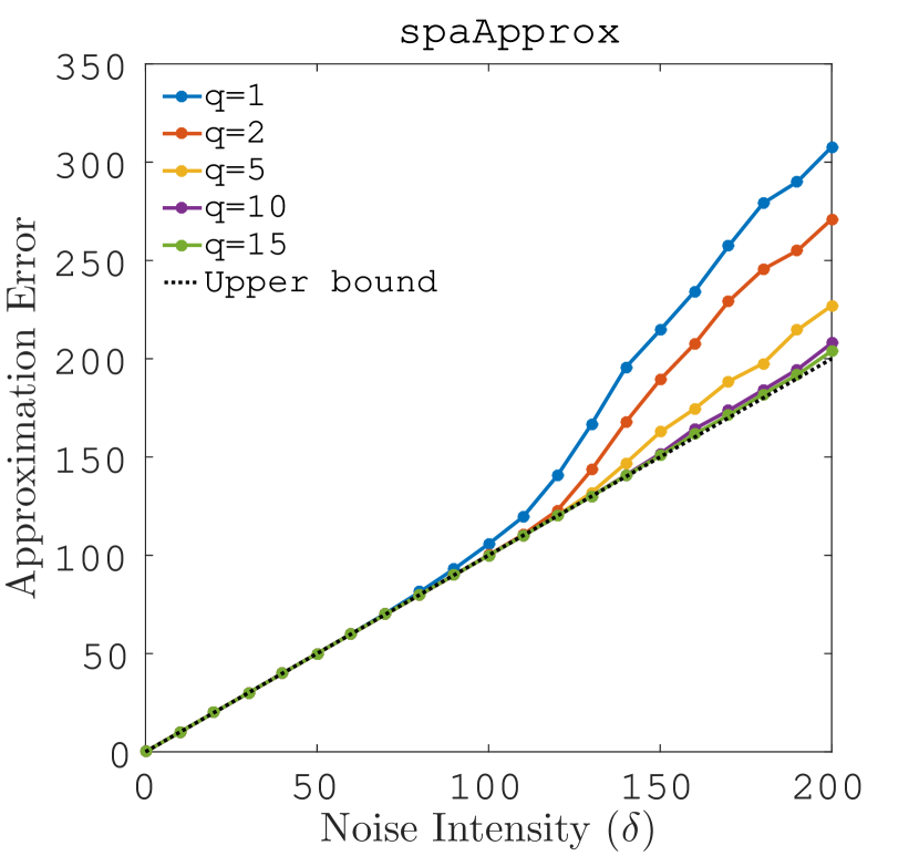
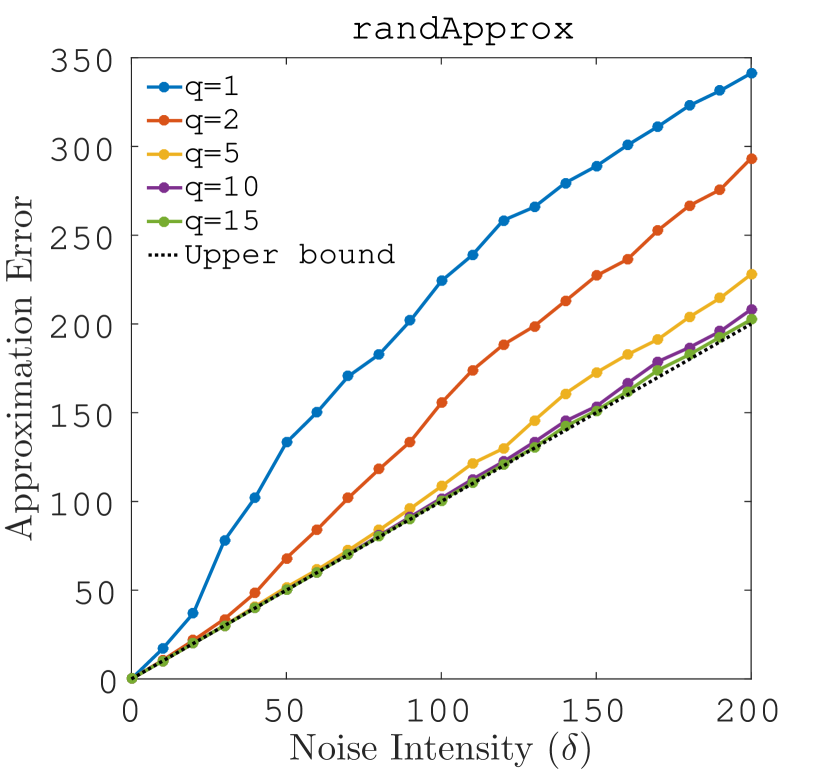
Figure 1: (Results of the first experiments) Approximation error of $\mathsf{spaApprox}$ (left) and $\mathsf{randApprox}$ (right) for noisy separable matrices of size $(d,m,k)=(500,100~{}000,10)$ with $\delta\in\{0,10,\ldots,200\}$.

The second experiments ran $\mathsf{mpspa}$, $\mathsf{spa}$, $\mathsf{pspa}$, $\mathsf{merspa}$ and $\mathsf{erspa}$ on the same data sets as in the first experiments. In the runs of $\mathsf{mpspa}$ and $\mathsf{merspa}$, $q$ was set from $1,2,5,10$ to $15$. To measure the robustness of each algorithm, we computed the recovery rate $\frac{1}{k}|\mathcal{I}\cap\mathcal{I}^{*}|$. Here, $\mathcal{I}$ is the index set returned by the algorithm and $\mathcal{I}^{*}$ is the set of column indices in $\bm{A}$ that correspond to the columns of $\bm{F}$. Figure 2 displays the average recovery rates of the algorithms. We can see that the recovery rates of $\mathsf{mpspa}$ increase with $q$. When $q$ exceeds $10$, the recovery rates of $\mathsf{mpspa}$ approach those of $\mathsf{pspa}$. These results imply that, even if the amount of noise is large, $\mathsf{mpspa}$ with a $q$ larger than $10$ is significantly more robust than $\mathsf{spa}$. The recovery rates of $\mathsf{merspa}$ show a similar tendency to those of $\mathsf{mpspa}$. We can hence see that $\mathsf{spaApprox}$ is useful for preprocessing in $\mathsf{erspa}$.

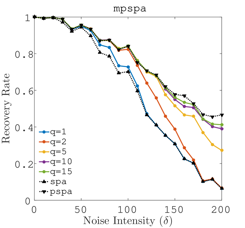
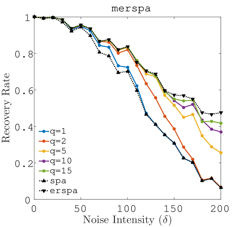
Figure 2: (Results of the second experiments) Recovery rate of $\mathsf{mpspa}$ (left) and $\mathsf{merspa}$ (right). The experiments used the same data sets as in the first experiments.

The third experiments used two types of data sets: data sets where $d$ and $k$ were fixed while $m$ was varied such that $(d,k)=(500,10)$ and $m\in\{300~{}000,400~{}000,500~{}000\}$, and data sets where $m$ and $k$ were fixed while $d$ was varied such that $(m,k)=(100~{}000,10)$ and $d\in\{1~{}000,2~{}000,3~{}000\}$. The noise intensity $\delta$ was set as $200$, and the value was the same for all the data sets. A single data set consisted of $50$ distinct noisy separable matrices for each $m$ and each $d$, and a total of $6$ data sets were used. We ran $\mathsf{spaApprox}$ and $\mathsf{randApprox}$ on the data sets with $q$ set to $10$. We also ran $\mathsf{svdApprox}$ on them. We measured the elapsed time of the algorithms for each run by using the MATLAB commands tic and toc. We also evaluated the approximation errors of the algorithms. Table 2 summarizes the average elapsed time in seconds and the average approximation error on $50$ noisy separable matrices. The elapsed time is listed in the columns labeled “time”, and the average approximation error in those labeled “error”. The results for $\mathsf{spaApprox}$ and $\mathsf{randApprox}$ were obtained by setting $q$ to $10$. We can see that $\mathsf{spaApprox}$ is 18 to 86 times faster than $\mathsf{svdApprox}$ in elapsed time. The approximation errors of $\mathsf{spaApprox}$ and $\mathsf{svdApprox}$ coincide in the first four digits for three out of six data sets. Although the elapsed time of $\mathsf{spaApprox}$ is longer than that of $\mathsf{randApprox}$, the differences are within a reasonable range. The approximation errors of $\mathsf{spaApprox}$ are smaller than those of $\mathsf{randApprox}$.

Table 2: (Results of the third experiments) Elapsed time in seconds and approximation error of $\mathsf{spaApprox}$ with $q=10$, $\mathsf{randApprox}$ with $q=10$ and $\mathsf{svdApprox}$. The factorization rank $k$ and noise intensity $\delta$ in the data sets were set to $k=10$ and $\delta=200$.

		$\mathsf{spaApprox}$ with $q=10$		$\mathsf{randApprox}$ with $q=10$		$\mathsf{svdApprox}$
$d$	$m$	time (s)	error	time (s)	error	time (s)	error
500	300 000	6.0	$200.12$	5.0	$203.88$	109.4	$199.91$
500	400 000	8.0	$199.93$	6.8	$203.70$	365.4	$199.92$
500	500 000	10.1	$199.93$	8.7	$205.87$	598.6	$199.93$
1 000	100 000	3.6	$201.61$	3.0	$204.29$	128.5	$199.86$
2 000	100 000	7.1	$200.59$	5.9	$200.95$	329.8	$199.93$
3 000	100 000	10.5	$199.94$	8.8	$202.83$	906.8	$199.93$

6.2 Real Data – Application to Hyperspectral Unmixing

Hyperspectral unmixing is a process to identify constituent materials in a hyperspectral image of a scene. We shall see that it can be formulated as a separable NMF problem with noise. The following description follows the tutorials [6, 23]. A hyperspectral camera is an optical instrument to measure the spectra of materials in a scene. For instance, the AVIRIS (airborne visible/infrared imaging spectrometer) sensor developed by the Jet Propulsion Laboratory can scan materials in 224 spectral bands with wavelengths ranging from 400 nm to 2500 nm. Let $d$ be the number of spectral bands that a hyperspectral camera can measure. We associate $\bm{A}=[\bm{a}_{1},\ldots,\bm{a}_{m}]\in\mathbb{R}^{d\times m}$ with an image of a scene taken by the camera such that the total number of pixels is $m$. Here, $\bm{a}_{i}$ stores measured reflectance values at the $i$th pixel, and the $\ell$th element of $\bm{a}_{i}$ corresponds to the measured value at the $\ell$th band. A linear mixing model assumes that $\bm{a}_{1},\ldots,\bm{a}_{m}$ are generated by

$$\bm{a}_{i}=\sum_{j=1}^{k}w_{ji}\bm{f}_{j}+\bm{n}_{i},\ i=1,\ldots,m$$

where $\bm{f}_{j}\in\mathbb{R}^{d}$ is the spectrum of the $j$th constituent material in the scene, and the elements of $\bm{f}_{j}$ are usually nonnegative; $w_{ji}\in\mathbb{R}$ is the mixing rate of the $j$th material at the $i$th pixel and satisfies $w_{ji}\geq 0$ and $\sum_{j=1}^{k}w_{ji}=1$; and $\bm{n}_{i}\in\mathbb{R}^{d}$ is noise. We call $\bm{f}_{j}$ the endmember of the image and $w_{ji}$ the abundance of the endmember $\bm{f}_{j}$ at the $i$th pixel. In the linear mixing model, hyperspectral unmixing is a problem of extracting endmembers $\bm{f}_{1},\ldots,\bm{f}_{k}$ from $\bm{A}$. We say that the $j^{*}$th material has a pure pixel if there is a pixel containing only the spectrum $\bm{f}_{j^{*}}$ of the material. That is, there is an $i\in\{1,\ldots,m\}$ such that $w_{ji}=1$ for $j=j^{*}$ and $w_{ji}=0$ for $j\neq j^{*}$. It might be reasonable to assume that every endmember has a pure pixel. This is called the pure pixel assumption, and it is the same as the separability assumption explained in Section 1. Accordingly, hyperspectral unmixing under the pure pixel assumption is equivalent to solving separable NMF problems with noise. For a matrix $\bm{A}$ associated with an image, the columns $\bm{a}_{i_{1}},\ldots\bm{a}_{i_{k}}$ of $\bm{A}$ extracted by a separable NMF algorithm are the estimations of the endmembers. The abundances of $\bm{a}_{i_{1}},\ldots,\bm{a}_{ij}$ at some pixel are obtained by solving the problem of minimizing a convex quadratic function over a simplex.

We are interested in how well $\mathsf{mpspa}$ works for hyperspectral unmixing. First of all, we report the results of experiments that evaluated the accuracy of low-rank approximations by $\mathsf{spaApprox}$ for real hyperspectral images. The experiments used 6 hyperspectral image data: Cuprite, DC Mall, Indian Pine, Pavia University, Salinas and Urban. Table 3 summarizes the number of spectral bands, pixels and identified constituent materials in each image data. We removed water absorption and noisy bands from the original data. The number of bands in the table is that of the bands we actually used. These image data have been well studied and are publicly available at the websites indicated in the footnotes. In particular, we used the Cuprite and Urban data that had been processed for the experiments reported in [38].

Table 3: Hyperspectral image data used in the experiments.

	# bands we actually used $(d)$	# pixels $(m)$		# identified constituent materials $(k)$
Cuprite	188	47 500	($250\times 190)$	12
DC Mall	191	392 960	($1~{}280\times 307$)	7
Indian Pine	202	1 644 292	($2~{}678\times 614$)	59
Pavia University	103	207 400	($610\times 340$)	9
Salinas	204	111 104	($512\times 217$)	16
Urban	162	94 249	($307\times 307$)	4

The Cuprite data was taken over a cuprite mining area in Nevada, USA. The data we used was a subimage of the original one. It has $250\times 190$ pixels with 188 clean bands, and there are 12 minerals in the scene. The DC Mall data was taken over the Washington DC Mall, USA. It has $1~{}280\times 307$ pixels with 191 clean bands. The scene contains 7 materials. The Indian Pine data was taken over the Purdue University Agronomy Farm in West Lafayette, USA. We used full North-South AVIRIS flightline data. It has $2~{}678\times 614$ pixels with 202 clean bands. Although the original data has 220 bands, we used the data from which 18 noisy bands (104-108, 150-162) are removed. The scanned area covers 59 types of agricultural and forest areas. The Pavia University data was taken over the University of Pavia, Italy. It has $610\times 340$ pixels with 103 bands, and the scene contains 9 materials. Salinas data was taken over Salinas Valley, California, USA. It has $512\times 217$ with 204 clean bands and the scene contains 16 types of agricultural areas. The Urban data has $307\times 307$ pixels with 162 clean bands. Although the original data has 210 bands, we used the data from which 48 water absorption and noisy bands (1-4, 76, 87, 101-111, 136-153, 198-210) are removed. The scene contains 4 materials. The Cuprite, Indian Pine and Salinas data were acquired with the AVIRIS sensor; the DC Mall and Urban data with the HYDICE sensor; and the Pavia University data with the ROSIS sensor.

We ran $\mathsf{spaApprox}$ and $\mathsf{svdApprox}$ on the $6$ hyperspectral image data. The parameter $k$ of $\mathsf{spaApprox}$ and $\mathsf{svdApprox}$ was set to the number of identified constituent materials in each image. The parameter $q$ of $\mathsf{spaApprox}$ was set to $10$ or $20$. Since some images demonstrated that the accuracy of the rank-$k$ approximations by $\mathsf{spaApprox}$ with $q=10$ is not so high, we increased $q$ from $10$ to $20$. To measure the accuracy of a rank-$k$ approximation $\bm{B}$ to a matrix $\bm{A}$, we computed the relative approximation error $\|\bm{A}-\bm{B}\|_{2}/\|\bm{A}\|_{2}$.

Table 4 summarizes the experimental results. The columns with the label “time” list the elapsed time in seconds of the algorithms and those with the label “rel error” list the relative approximation error of the algorithms. We first observe the results for data except Indian Pine. When $q=10$, $\mathsf{spaApprox}$ is 5 to 9 times faster than $\mathsf{svdApprox}$ in elapsed time. The relative approximation errors of $\mathsf{spaApprox}$ and $\mathsf{svdApprox}$ coincide in the first four digits for Salinas and Urban, while there are no small gaps between them for Cuprite and DC Mall; in particular, only the first digits coincide for DC Mall. When $q=20$, the first three digits coincide for Cuprite and the first two digits coincide for DC Mall. Even if $q$ increases from 10 to 20, $\mathsf{spaApprox}$ still maintains an advantage in elapsed time over $\mathsf{svdApprox}$; it is 5 times faster on Cuprite and DC Mall. We next delve into the discussion of experiments on Indian Pine. Although $\mathsf{spaApprox}$ with $q=10$ and $20$ terminated normally and returned the output, the execution of $\mathsf{svdApprox}$ was forced to terminate by MATLAB before returning the output. The main reason why the execution was interrupted could be that it requested a large amount of memory. Indeed, we succeeded to run $\mathsf{svdApprox}$ on Indian Pine by using a desktop computer with more memory: it was equipped with Intel Core i7-5775R processor and 16 GB memory. The experiments revealed that the relative approximation error of $\mathsf{svdApprox}$ for Indian Pine is $4.7510\times 10^{-4}$.

Table 4: Elapsed time in seconds and relative approximation error of $\mathsf{spaApprox}$ with $q=10$ and $20$ and $\mathsf{svdApprox}$ for hyperspectral image data. The symbol “-” means that the execution of $\mathsf{svdApprox}$ was interrupted by MATLAB with an error message and was not terminated normally.

	$\mathsf{spaApprox}$ with $q=10$		$\mathsf{spaApprox}$ with $q=20$		$\mathsf{svdApprox}$
	time (s)	rel error	time (s)	rel error	time (s)	rel error
Cuprite	0.7	$2.1944\times 10^{-3}$	1.2	$2.1073\times 10^{-3}$	6.9	$2.1061\times 10^{-3}$
DC Mall	4.0	$8.3421\times 10^{-3}$	7.2	$8.1649\times 10^{-3}$	36.5	$8.1514\times 10^{-3}$
Indian Pine	81.1	$4.9211\times 10^{-4}$	150.0	$4.8687\times 10^{-4}$	-	-
Pavia University	1.7	$8.3077\times 10^{-3}$	3.1	$8.3062\times 10^{-3}$	10.8	$8.3062\times 10^{-3}$
Salinas	2.1	$1.3354\times 10^{-3}$	3.8	$1.3351\times 10^{-3}$	20.6	$1.3351\times 10^{-3}$
Urban	0.6	$2.2364\times 10^{-2}$	1.1	$2.2364\times 10^{-2}$	3.3	$2.2364\times 10^{-2}$

Next, we report the results of experiments examining the accuracy of the endmembers estimated by $\mathsf{mpspa}$ for a hyperspectral image. The experiments used the Urban data. Figure 3 displays an RGB image of the data. The constituent materials in the image scene were examined in the previous studies [38, 22, 36], and 4 materials were identified: asphalt, grass, tree and roof. The spectra of those materials are available from the first author’s website of [38] (footnote 3). We supposed that each of them was a true endmember in the Urban data. To measure the accuracy of the estimated endmembers, we evaluated a spectral angle distance (SAD). Given a true endmember $\bm{f}\in\mathbb{R}^{d}$ and an estimated endmember $\widehat{\bm{f}}\in\mathbb{R}^{d}$, it is computed as $\arccos(\bm{f}^{\top}\widehat{\bm{f}}/\|\bm{f}\|_{2}\|\widehat{\bm{f}}\|_{2})$. SAD takes values between $0$ and $1$. A small SAD value means that an estimated endmember is close to a true endmember, while a large SAD value means the opposite. We set $k$ as $4$ and ran $\mathsf{mpspa}$ on a matrix associated with the Urban data. For comparison, we also ran $\mathsf{pspa}$, $\mathsf{spa}$, $\mathsf{spaspa}$, and $\mathsf{vca}$.

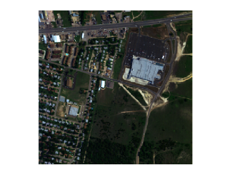
Figure 3: RGB image of Urban data generated by the satellite image processing software ENVI.

We examined the output of $\mathsf{mpspa}$ for increasing $q$. When $q=4$, it coincided with the output of $\mathsf{pspa}$. At that point, the relative error of $\mathsf{spaApprox}$ was $2.2587\times 10^{-2}$, and there was still a gap between the accuracies of the rank-$k$ approximations by $\mathsf{spaApprox}$ and $\mathsf{svdApprox}$. Nevertheless, $\mathsf{mpspa}$ returned the same output as $\mathsf{pspa}$. The elapsed time of $\mathsf{mpspa}$ with $q=4$ was 2.3 seconds, while that of $\mathsf{pspa}$ was 6.4 seconds.

Table 5 summarizes the SADs of the algorithms. The rows correspond to the estimated endmembers, and values in each row are the SADs for the spectra of the corresponding materials. We underlined the minimum value on each row. The estimated endmember is the closest to the spectrum of a material corresponding to the underlined value. We can see that the endmembers estimated by $\mathsf{mpspa}$ with $q=4$ and $\mathsf{pspa}$ are close to the spectra of 4 materials, respectively. However, the estimates of the other algorithms are far from the spectrum of grass. We computed the abundance maps of true and estimated endmembers. We let the abundance maps of the true endmembers be the ground truth of the Urban data. Figure 4 displays the ground truth and the abundance maps obtained by the algorithms. A pixel color is white when the abundance of the corresponding material is large, and the color gradually turns to black as the abundance gets smaller. This enables us to visually confirm that the abundance maps for $\mathsf{mpspa}$ with $q=4$ and $\mathsf{pspa}$ well match the ground truth.

Table 5: SAD of $\mathsf{mpspa}$ with $q=4$ and $\mathsf{pspa}$ (upper-left), $\mathsf{spa}$ (upper-right), $\mathsf{spaspa}$ (lower-left) and $\mathsf{vca}$ (lower-right). The rows correspond to the estimated endmembers. The underlined value indicates the minimum value on each row.

$\mathsf{mpspa}$ with $q=4$ and $\mathsf{pspa}$
	asphalt	grass	tree	roof
1	0.191	0.594	0.988	0.553
2	0.489	0.045	0.435	0.606
3	0.852	0.465	0.074	0.816
4	0.564	0.653	0.783	0.217

$\mathsf{spa}$
	asphalt	grass	tree	roof
1	0.132	0.469	0.858	0.497
2	0.564	0.653	0.783	0.217
3	0.852	0.465	0.074	0.816
4	1.156	1.367	1.443	0.874

$\mathsf{spaspa}$
	asphalt	grass	tree	roof
1	0.191	0.594	0.988	0.553
2	0.564	0.653	0.783	0.217
3	0.852	0.465	0.074	0.816
4	1.156	1.367	1.443	0.874

$\mathsf{vca}$
	asphalt	grass	tree	roof
1	0.228	0.670	1.049	0.535
2	0.884	0.574	0.530	0.817
3	0.970	0.678	0.300	0.818
4	1.153	1.369	1.449	0.867

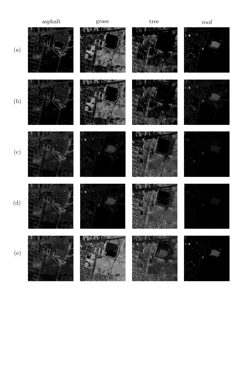
Figure 4: Ground truth and abundance maps obtained by the algorithms: (a) ground truth, (b) $\mathsf{mpspa}$ with $q=4$ and $\mathsf{pspa}$, (c) $\mathsf{spa}$, (d) $\mathsf{spaspa}$, and (e) $\mathsf{vca}$. From left to right, panels in (a) display the abundance maps of the true endmembers, asphalt, grass, tree and roof, respectively. From left to right, panels in (b) to (e) display the abundance maps of the estimated endmembers shown in Table 5 from top to bottom.

7 Summary and Future Research

We have proposed a modification to PSPA, and described it in Algorithm 4. The modification was motivated by addressing the cost issue of PSPA. Although PSPA uses the best rank-$k$ approximation to an input matrix, the modification avoids having to use it and alternatively uses a rank-$k$ approximation produced by Algorithm 1. We evaluated the computational cost of Algorithm 1 and clarified that it is low. The robustness to noise of Algorithm 4 depends on the approximation accuracy of Algorithm 1. We derived a bound on the approximation error $\|\bm{A}-\bm{B}\|_{2}$ for the input matrix $\bm{A}$ and the output matrix $\bm{B}$ of Algorithm 1 and described the result in Theorem 3. We conducted an empirical study to assess the actual performance of Algorithm 1 and Algorithm 4.

Finally, we suggest the directions of study for future research.

• In Theorem 3, we put conditions in which an input matrix is noisy separable and the amount of noise is small and then derived a bound on the approximation error of Algorithm 1. Further study is needed to see whether it is possible to obtain the error bound under weaker conditions. In relation to this, it would be interesting to explore how well Algorithm 1 works for a general matrix from theoretical and practical perspectives.

• Theorem 3 implies that Algorithm 1 can produce highly accurate low-rank approximations if the value of an input parameter $q$ is set as a large integer. However, the theorem may not help us to estimate a parameter value required for obtaining such low-rank approximations. This is because the theorem describes a bound on the approximation error of Algorithm 1 by using the ratio between the $(k+1)$th and $k$th largest singular values of an input matrix $\bm{A}$. Regarding Algorithm 5, the author of [37] has derived the following error bound. It is different from an error bound shown in [18] that we saw in Section 5.3. Theorem 4.16 in [37] argues that, given a matrix $\bm{A}\in\mathbb{R}^{d\times m}$ and integers $q$ and $k$, Algorithm 5 returns a rank-$k$ approximation $\bm{B}$ to $\bm{A}$ satisfying $\|\bm{A}-\bm{B}\|_{2}\leq\sigma_{k+1}(c(m-k)/k)^{1/4q+2}$ with probability at least $4/5$ where $c$ is a positive real number. This theoretical result can help us to estimate the value of $q$ before running Algorithm 5. If we desire to obtain a rank-$k$ approximation $\bm{B}$ to $\bm{A}$ satisfying $\|\bm{A}-\bm{B}\|_{2}\leq(1+\epsilon)\sigma_{k+1}$, the result tells us that $q$ should be set as an integer determined by $\epsilon$, $c$, $m$ and $k$. It would be interesting to investigate whether we can obtain this type of an error bound even in case of Algorithm 1. Also, further experimental study would be needed to observe the relation between the accuracy of low-rank approximation by Algorithm 1 and a paramenter $q$.

• As mentioned in Remark 2, the original algorithm description of the randomized subspace iteration [30, 20, 18] includes an input parameter $\ell$. Similarly, Algorithm 1 can be extended to include a parameter $\ell$. The extension would probably enable Algorithm 1 to improve the approximation error by increasing $\ell$ as well as $q$. On the other hand, there is a concern that the extension involves a computation of a truncated SVD; the computational cost becomes large as $\ell$ increases. It would be interesting to see whether the extended algorithm has any advantage in the modification of PSPA.

Appendix  Proof of Lemma 3(a)

Here, we prove Lemma 3(a). The proof follows straightforwardly from the arguments in the proof of Theorem 9.1 in [20]. The notation $\bm{A}\preceq\bm{B}$ below means that $\bm{B}-\bm{A}$ is positive semidefinite.

Lemma 4.

If $\bm{A}\preceq\bm{B}$, then $\|\bm{A}\|_{2}\leq\|\bm{B}\|_{2}$.

This inequality follows from the definition of a positive semidefinite matrix and the property that a symmetric matrix $\bm{A}$ has the relation $\|\bm{A}\|_{2}=\max_{\|\bm{x}\|_{2}=1}\bm{x}^{\top}\bm{A}\bm{x}$.

Lemma 5 (Proposition 8.3 in [20] and also Lemma 1.1 in [7]).

Let $\bm{A}$ be a symmetric matrix written in the blocks

$$\bm{A}=\left[\begin{array}[]{cc}\bm{X}&\bm{Z}\\ \bm{Z}^{\top}&\bm{Y}\end{array}\right],$$

and suppose that $\bm{A}$ is positive semidefinite. Then, $\|\bm{A}\|_{2}\leq\|\bm{X}\|_{2}+\|\bm{Y}\|_{2}$.

(Proof of Lemma 3(a)).

We have $\|(\bm{I}-\bm{P}_{\bm{Z}})\bm{\Sigma}\|_{2}^{2}=\|\bm{\Sigma}^{\top}(\bm{I}-\bm{P}_{\bm{Z}})\bm{\Sigma}\|_{2}$ since $\bm{I}-\bm{P}_{\bm{Z}}$ is an orthogonal projection and thus satisfies $\bm{I}-\bm{P}_{\bm{Z}}=(\bm{I}-\bm{P}_{\bm{Z}})^{\top}$ and $\bm{I}-\bm{P}_{\bm{Z}}=(\bm{I}-\bm{P}_{\bm{Z}})^{2}$. Below, we derive an upper bound on $\|\bm{\Sigma}^{\top}(\bm{I}-\bm{P}_{\bm{Z}})\bm{\Sigma}\|_{2}$. As seen in the proof of Lemma 3(b), from the nonsingularity of $\bm{Z}_{1}$, we can write $\bm{Z}$ as

$$\bm{Z}=\left[\begin{array}[]{c}\bm{Z}_{1}\\ \bm{Z}_{2}\end{array}\right]\\ =\left[\begin{array}[]{c}\bm{I}\\ \bm{H}\end{array}\right]\bm{Z}_{1}\ \mbox{and}\ \bm{H}=\bm{Z}_{2}\bm{Z}_{1}^{-1}.$$

Then,

$$\bm{P}_{\bm{Z}}=\bm{Z}(\bm{Z}^{\top}\bm{Z})^{-1}\bm{Z}^{\top}=\left[\begin{array}[]{cc}(\bm{I}+\bm{H}^{\top}\bm{H})^{-1}&(\bm{I}+\bm{H}^{\top}\bm{H})^{-1}\bm{H}^{\top}\\ \bm{H}(\bm{I}+\bm{H}^{\top}\bm{H})^{-1}&\bm{H}(\bm{I}+\bm{H}^{\top}\bm{H})^{-1}\bm{H}^{\top}\end{array}\right].$$

The following matrix inequalities hold.

$$\bm{I}-(\bm{I}+\bm{H}^{\top}\bm{H})^{-1}\preceq\bm{H}^{\top}\bm{H}\ \mbox{and}\ \bm{I}-\bm{H}(\bm{I}+\bm{H}^{\top}\bm{H})^{-1}\bm{H}^{\top}\preceq\bm{I}.$$

The first one can be checked by considering the SVD of $\bm{H}$; see also Proposition 8.2 of [20]. The second one comes from the fact that $\bm{H}(\bm{I}+\bm{H}^{\top}\bm{H})^{-1}\bm{H}^{\top}$ is positive semidefinite. From those inequalities, we get

$$\bm{I}-\bm{P}_{\bm{Z}}\preceq\left[\begin{array}[]{cc}\bm{H}^{\top}\bm{H}&-(\bm{I}+\bm{H}^{\top}\bm{H})^{-1}\bm{H}^{\top}\\ -\bm{H}(\bm{I}+\bm{H}^{\top}\bm{H})^{-1}&\bm{I}\end{array}\right]$$

and this implies

$$\bm{\Sigma}^{\top}(\bm{I}-\bm{P}_{\bm{Z}})\bm{\Sigma}\preceq\bm{\Sigma}^{\top}\left[\begin{array}[]{cc}\bm{H}^{\top}\bm{H}&-(\bm{I}+\bm{H}^{\top}\bm{H})^{-1}\bm{H}^{\top}\\ -\bm{H}(\bm{I}+\bm{H}^{\top}\bm{H})^{-1}&\bm{I}\end{array}\right]\bm{\Sigma}.$$ (25)

$\bm{I}-\bm{P}_{\bm{Z}}$ is positive semidefinite, since it is an orthogonal projection. This means that the matrix on the left side of (25) is positive semidefinite, and hence so is the matrix on the right side. The right-side matrix takes the following form. If $d\geq m$,

$$\left[\begin{array}[]{c|ccc}\bm{S}_{1}\bm{H}^{\top}\bm{H}\bm{S}_{1}&&\ast&\\ \hline\cr&\sigma_{k+1}^{2}&&\\ \ast&&\ddots&\\ &&&\sigma_{m}^{2}\\ \end{array}\right]\in\mathbb{R}^{m\times m}.$$

Otherwise,

$$\left[\begin{array}[]{c|ccccccc}\bm{S}_{1}\bm{H}^{\top}\bm{H}\bm{S}_{1}&&&\ast&&\\ \hline\cr&\sigma_{k+1}^{2}&&&&&\\ &&\ddots&&&&\\ \ast&&&\sigma_{d}^{2}&&&\\ &&&&0&&\\ &&&&&\ddots&\\ &&&&&&0\\ \end{array}\right]\in\mathbb{R}^{m\times m}.$$

Here, $\bm{S}_{1}$ is the $k\times k$ upper block of a diagonal matrix $\bm{S}$ whose elements are given as (9); that is, the diagonal elements $s_{1},\ldots,s_{k}$ of $\bm{S}_{1}$ correspond to those $\sigma_{1},\ldots,\sigma_{k}$ of $\bm{\Sigma}$. Accordingly, from Lemmas 4 and 5, we obtain $\|(\bm{I}-\bm{P}_{\bm{Z}})\bm{\Sigma}\|_{2}^{2}=\|\bm{\Sigma}^{\top}(\bm{I}-\bm{P}_{\bm{Z}})\bm{\Sigma}\|_{2}\leq\|\bm{H}\bm{S}_{1}\|_{2}^{2}+\sigma_{k+1}^{2}$.

∎

References

- [1] S. D. Ahipasaoglu, P. Sun, and M. J. Todd. Linear convergence of a modified Frank-Wolfe algorithm for computing minimum-volume enclosing ellipsoids. Optimization Methods and Software, 23(1):5–19, 2008.
- [2] U. M. C. Araújo, B. T. C. Saldanha, R. K. H. Galvão, T. Yoneyama, H. C. Chame, and V. Visani. The successive projections algorithm for variable selection in spectroscopic multicomponent analysis. Chemometrics and Intelligent Laboratory Systems, 57(2):65–73, 2001.
- [3] S. Arora, R. Ge, Y. Halpern, D. Mimno, and A. Moitra. A practical algorithm for topic modeling with provable guarantees. In Proceedings of the 30th International Conference on Machine Learning (ICML), 2013.
- [4] S. Arora, R. Ge, R. Kannan, and A. Moitra. Computing a nonnegative matrix factorization – Provably. In Proceedings of the 44th symposium on Theory of Computing (STOC), pages 145–162, 2012.
- [5] S. Arora, R. Ge, and A. Moitra. Learning topic models – Going beyond SVD. In Proceedings of the 53rd Annual Symposium on Foundations of Computer Science (FOCS), pages 1–10, 2012.
- [6] J. M. Bioucas-Dias, A. Plaza, N. Dobigeon, M. Parente, Q. Du, P. Gader, and J. Chanussot. Hyperspectral unmixing overview: Geometrical, statistical, and sparse regression-based approaches. IEEE Journal of Selected Topics in Applied Earth Observations and Remote Sensing, 5(2):354–379, 2012.
- [7] J.-C. Bourin, E.-Y. Lee, and M. Lin. On a decomposition lemma for positive semi-definite block-matrices. Linear Algebra and its Applications, 437:1906–1912, 2012.
- [8] S. Boyd and L. Vandenberghe. Convex Optimization. Cambridge University Press, 2004.
- [9] P. Businger and G. H. Golub. Linear least squares solutions by Householder transformations. Numerische Mathematik, 7(3):269–276, 1965.
- [10] E. Candès and Y. Plan. Matrix completion with noise. Proceedings of the IEEE, 98(6):925–936, 2010.
- [11] A. Çivril and M. Magdon-Ismail. On selecting a maximum volume sub-matrix of a matrix and related problems. Theoretical Computer Science, 410:4801––4811, 2009.
- [12] D. Donoho and V. Stodden. When does non-negative matrix factorization give a correct decomposition into parts? In Proceedings of Advances in Neural Information Processing Systems 16 (NIPS), pages 1141–1148, 2003.
- [13] C. Eckart and G. Young. The approximation of one matrix by another of lower rank. Psychometrika, 1(3):211–218, 1936.
- [14] N. Gillis and W. K. Ma. Enhancing pure-pixel identification performance via preconditioning. SIAM Journal on Imaging Sciences, 8(2):1161–1186, 2015.
- [15] N. Gillis and S. A. Vavasis. Fast and robust recursive algorithms for separable nonnegative matrix factorization. IEEE Transactions on Pattern Analysis and Machine Intelligence, 36(4):698–714, 2014.
- [16] N. Gillis and S. A. Vavasis. Semidefinite programming based preconditioning for more robust near-separable nonnegative matrix factorization. SIAM Journal on Optimization, 25(1):677–698, 2015.
- [17] G. H. Golub and C. F. V. Loan. Matrix Computation. The Johns Hopkins University Press, 4th edition, 2013.
- [18] M. Gu. Subspace iteration randomization and singular value problems. SIAM Journal on Scientific Computing, 37(3):A1139––A1173, 2015.
- [19] S. Gunasekar, A. Acharya, N. Gaur, and J. Ghosh. Noisy matrix completion using alternating minimization. In Proceedings of the European Conference on Machine Learning and Principles and Practice of Knowledge Discovery in Databases (ECML PKDD), pages 194–209, 2013.
- [20] N. Halko, P. G. Martinsson, and J. A. Tropp. Finding structure with randomness: Probabilistic algorithms for constructing approximate matrix decomposions. SIAM Review, 53(2):217–288, 2011.
- [21] R. H. Keshavan, A. Montanari, and S. Oh. Matrix completion from noisy entrie. Journal of Machine Learning Research, 11:2057–2078, 2010.
- [22] X. Lu, H. Wu, and Y. Yuan. Double constrained NMF for hyperspectral unmixing. IEEE Transactions on Geoscience and Remote Sensing, 52(5):2746–2758, 2014.
- [23] W.-K. Ma, J. M. Bioucas-Dias, T.-H. Chan, N. Gillis, P. Gader, A. J. Plaza, A. Ambikapathi, and C.-Y. Chi. A signal processing perspective on hyperspectral unmixing: Insights from remote sensing. IEEE Signal Processing Magazine, 31(2):67–81, 2014.
- [24] C. D. Manning, P. Raghavan, and H. Schuetze. Introduction to Information Retrieval. Cambridge University Press, 2008.
- [25] A. K. Menon and C. Elkan. Fast algorithms for approximating the singular value decomposition. ACM Transactions on Knowledge Discovery from Data, 5(2):13:1–13:36, 2011.
- [26] T. Mizutani. Ellipsoidal rounding for nonnegative matrix factorization under noisy separability. Journal of Machine Learning Research, 15:1011–1039, 2014.
- [27] T. Mizutani. Robustness analysis of preconditioned successive projection algorithm for general form of separable NMF problem. Linear Algebra and its Applications, 497:1–22, 2016.
- [28] J. M. P. Nascimento and J. M. B. Dias. Vertex component analysis: A fast algorithm to unmix hyperspectral data. IEEE Transactions on Geoscience and Remote Sensing, 43(4):898–910, 2005.
- [29] C. H. Papadimitriou, P. Raghavan, H. Tamaki, and S. Vempala. Latent semantic indexing: A probabilistic analysis. Journal of Computer and System Sciences, 61:217–235, 2000.
- [30] V. Rokhlin, A. Szlam, and M. Tygert. A randomized algorithm for principal component analysis. SIAM Journal on Matrix Analysis and Applications, 31(3):1100–1124, 2009.
- [31] P. Sun and R. M. Freund. Computation of minimum-volume covering ellipsoids. Operations Research, 52(5):690–706, 2004.
- [32] M. Tepper and G. Sapiro. Compressed nonnegative matrix factorization is fast and accurate. IEEE Transactions on Signal Processing, 64(9):2269–2283, 2016.
- [33] K.-C. Toh, M. J. Todd, and R. H. Tütüncü. SDPT3 – a MATLAB software package for semidefinite programming. Optimization Methods and Software, 11:545–581, 1999.
- [34] L. N. Trefethen and D. Bau, III. Numerical Linear Algebra. SIAM, 1997.
- [35] S. A. Vavasis. On the complexity of nonnegative matrix factorization. SIAM Journal of Optimization, 20(3):1364–1377, 2009.
- [36] Y. Wang, C. Pan, S. Xiang, and F. Zhu. Robust hyperspectral unmixing with correntropy-based metric. IEEE Transactions on Image Processing, 24(11):4027–4040, 2015.
- [37] D. P. Woodruff. Sketching as a tool for numerical linear algebra. Foundations and Trends in Theoretical Computer Science, 10(1–2):1––157, 2014.
- [38] F. Zhu, Y. Wang, B. Fan, S. Xiang, G. Meng, and C. Pan. Spectral unmixing via data-guided sparsity. IEEE Transactions on Image Processing, 23(12):5412–5427, 2014.