Randomized Complete Pivoting for Solving
Symmetric Indefinite Linear Systemsthanks: Supported by CSC (grant 201606310121).

Yuehua Feng School of Mathematical Science, Xiamen University, China. E-mail: fyh1001@hotmail.com.    Jianwei Xiao Department of Mathematics, University of California, Berkeley. E-mail: jwxiao@berkeley.edu.    Ming Gu Department of Mathematics, University of California, Berkeley. E-mail: mgu@math.berkeley.edu.
Abstract

The Bunch-Kaufman algorithm and Aasen’s algorithm are two of the most widely used methods for solving symmetric indefinite linear systems, yet they both are known to suffer from occasional numerical instability due to potentially exponential element growth or unbounded entries in the matrix factorization. In this work, we develop a randomized complete pivoting (RCP) algorithm for solving symmetric indefinite linear systems. RCP is comparable to the Bunch-Kaufman algorithm and Aasen’s algorithm in computational efficiency, yet enjoys theoretical element growth and bounded entries in the factorization comparable to that of complete-pivoting, up to a theoretical failure probability that exponentially decays with an oversampling parameter. Our finite precision analysis shows that RCP is as numerically stable as Gaussian elimination with complete pivoting, and RCP has been observed to be numerically stable in our extensive numerical experiments.

Keywords: symmetric indefinite matrix, diagonal pivoting, randomized matrix algorithms, block LDLT𝐿𝐷superscript𝐿𝑇LDL^{T} factorization

AMS subject classifications. 15A06, 15A23, 65F05

1 Introduction

A symmetric matrix An×n𝐴superscript𝑛𝑛A\in\mathbb{R}^{n\times n} is said to be indefinite if it has both positive and negative eigenvalues. Its corresponding linear system Ax=b𝐴𝑥𝑏Ax=b is called a symmetric indefinite linear system. Such symmetric indefinite linear systems appear in various problems coming from acoustics, electromagnetism, and physics of structures [34]. Symmetric indefinite linear systems are also widely solved in linear least squares problems [10] and saddle point problems [9].

To effectively solve symmetric indefinite linear systems when A𝐴A is a dense matrix, there are four well-known algorithms: Bunch-Parlett algorithm [14], Bunch-Kaufman algorithm [13], bounded Bunch-Kaufman algorithm [5], and Aasen’s algorithm [1]. Duff and Reid’s multifrontal algorithm [20] and Liu’s sparse threshold algorithm [30] can be used to solve sparse symmetric indefinite linear systems. All but Aasen’s algorithm use diagonal pivoting to factorize A𝐴A into block LDLT𝐿𝐷superscript𝐿𝑇LDL^{T}, where L𝐿L is unit lower triangular and D𝐷D is symmetric block diagonal with each block of order 111 or 222. Aasen’s algorithm factorizes A𝐴A into LTLT𝐿𝑇superscript𝐿𝑇LTL^{T}, where T𝑇T is a symmetric tridiagonal matrix.

The block LDLT𝐿𝐷superscript𝐿𝑇LDL^{T} factorization is a generalization of the Cholesky factorization, which requires the input matrix A𝐴A to be positive semi-definite. While the Cholesky factorization is numerically stable with or without diagonal pivoting [21], block LDLT𝐿𝐷superscript𝐿𝑇LDL^{T} factorization with partial pivoting can have numerical instability issues [5, 24]. There are a number of strategies to choose permutation matrices for numerical stability. Bunch and Parlett [14] proposed a complete pivoting strategy, which requires searching the whole Schur complement at each stage of the block LDLT𝐿𝐷superscript𝐿𝑇LDL^{T} factorization and therefore requires up to O(n3)𝑂superscript𝑛3O(n^{3}) comparisons. Bunch [12] proved that Bunch-Parlett algorithm satisfies a backward error bound almost as good as that for Gaussian elimination with complete pivoting (GECP), and its element growth factor is within a factor 3.07(n1)0.4463.07superscript𝑛10.4463.07(n-1)^{0.446} of Wilkinson’s element growth factor bound [38] for GECP. To reduce the number of comparisons, Bunch and Kaufman devised a partial pivoting strategy, which searches at most two columns at each stage and the number of comparisons is reduced from O(n3)𝑂superscript𝑛3O(n^{3}) to O(n2)𝑂superscript𝑛2O(n^{2}). However, the multipliers can’t be controlled with Bunch-Kaufman partial pivoting strategy. To overcome this instability problem, Ashcraft, Grimes, and Lewis [5] proposed a bounded Bunch-Kaufman algorithm, where multipliers can be bounded near one, at a potentially high cost in comparisons. In the worst-case scenario, bounded Bunch-Kaufman is no better than the Bunch-Parlett algorithm, while in the best-case scenario bounded Bunch-Kaufman costs no more than the Bunch-Kaufman algorithm. LAPACK [2] routines SYSV and SYSVX, and LINPACK [17] routines SIFA and SISL are all based on the Bunch-Kaufman algorithm, whereas LAPACK routines SYSV__\_rook and SYSV__\_aa are based on bounded Bunch-Kaufman algorithm and Aasen’s algorithm respectively.

Randomization techniques are gaining increasing popularity in numerical linear algebra. Application of randomization in numerical linear algebra includes computing condition estimates [3, 29], solving linear systems using Monte Carlo methods [16] and Random Butterfly Transformation [6, 7, 8, 36]. Random projection is one important tool among randomization techniques. Random projections [4, 37], a technique of projecting a set of points from a higher-dimensional space to a randomly chosen lower-dimensional space, approximately preserve pairwise distances [28] with high probability. Random projections have proven themselves very effective tool in numerical linear algebra [22, 23, 31, 32, 33, 39, 40].

In this paper, we employ random projection techniques to develop a novel pivoting strategy called randomized complete pivoting (RCP). Comparing with the Bunch-Kaufman algorithm and Aasen’s algorithm, the RCP algorithm requires a relatively small random projection related overhead that diminishes with matrix dimensions. However, we show that the element growth factor upper bound for the RCP algorithm is comparable to those for GECP and the Bunch-Parlett algorithm. Additionally, we performed an error analysis on the RCP algorithm to demonstrate its numerical stability.

This paper is organized as follows. Section 2 introduces the preliminaries and background. Section 3 presents the RCP algorithm, its implementations and a floating point operations count analysis. Section 4 includes analyses of the RCP algorithm, including reliability analysis of randomized column pivots, analysis on element growth and column growth, and finite precision analysis. In Section 5, we report results from our extensive numerical experiments of the RCP algorithm, which demonstrate its effectiveness and reliability as claimed. Finally we draw some conclusions in Section 6.

2 Preliminaries and Background

In this section, we introduce some basic notation as well as the Bunch-Kaufman algorithm.

2.1 Preliminaries

Let p\|\cdot\|_{p} and q\|\cdot\|_{q} be two vector norms, their corresponding subordinate matrix norm of a given matrix A=(ai,j)m×n𝐴subscript𝑎𝑖𝑗superscript𝑚𝑛A=\left(a_{i,j}\right)\in\mathbb{R}^{m\times n} is [25, 27]

Ap,q=def𝐬𝐮𝐩0xnAxqxp=𝐦𝐚𝐱xp=1Axq.superscript𝑑𝑒𝑓subscriptnorm𝐴𝑝𝑞subscript𝐬𝐮𝐩0𝑥superscript𝑛subscriptnorm𝐴𝑥𝑞subscriptnorm𝑥𝑝subscript𝐦𝐚𝐱subscriptnorm𝑥𝑝1subscriptnorm𝐴𝑥𝑞\|A\|_{p,q}\stackrel{{\scriptstyle def}}{{=}}{\bf sup}_{0\neq x\in\mathbb{R}^{n}}\frac{\|Ax\|_{q}}{\|x\|_{p}}={\bf max}_{\|x\|_{p}=1}\|Ax\|_{q}.

The following cases [25] will be of special use to us:

A1,2=𝐦𝐚𝐱1inA(:,i)2,A1,=𝐦𝐚𝐱i,j|ai,j|,formulae-sequencesubscriptnorm𝐴12subscript𝐦𝐚𝐱1𝑖𝑛subscriptnorm𝐴:𝑖2subscriptnorm𝐴1subscript𝐦𝐚𝐱𝑖𝑗subscript𝑎𝑖𝑗\displaystyle\left\|A\right\|_{1,2}={\bf max}_{1\leq i\leq n}\left\|A(:,i)\right\|_{2},\quad\left\|A\right\|_{1,\infty}={\bf max}_{i,j}|a_{i,j}|,
AB1,2A2B1,2,AB1,2A1,2B1,formulae-sequencesubscriptnorm𝐴𝐵12subscriptnorm𝐴2subscriptnorm𝐵12subscriptnorm𝐴𝐵12subscriptnorm𝐴12subscriptnorm𝐵1\displaystyle\left\|AB\right\|_{1,2}\leq\left\|A\right\|_{2}\left\|B\right\|_{1,2},\quad\left\|AB\right\|_{1,2}\leq\left\|A\right\|_{1,2}\left\|B\right\|_{1},

where Am×k𝐴superscript𝑚𝑘A\in\mathbb{R}^{m\times k} and Bk×n𝐵superscript𝑘𝑛B\in\mathbb{R}^{k\times n}.

As in the original work of Wilkinson on GECP [38], Hadamard’s inequality [27] will prove useful in our element growth analysis as well.

Theorem 2.1.

Let An×n𝐴superscript𝑛𝑛A\in\mathbb{R}^{n\times n}, then

|det(A)|j=1nA(:,j)2.𝐴superscriptsubscriptproduct𝑗1𝑛subscriptnorm𝐴:𝑗2\left|\det(A)\right|\leq\prod_{j=1}^{n}\left\|A(:,j)\right\|_{2}.

Lemma 2.1 is a much weakened version of the original Johnson-Lindenstrauss Lemma [28, 37]. It has proven itself indispensable in the study of randomized numerical linear algebra [33, 40].

Lemma 2.1.

Let xn𝑥superscript𝑛x\in\mathbb{R}^{n} and 0<ϵ<10italic-ϵ10<\epsilon<1. Assume that entries in Ωp×nΩsuperscript𝑝𝑛\Omega\in\mathbb{R}^{p\times n} are independent and identically distributed (i.i.d.) random variables drawn from 𝒩(0,1)𝒩01\mathcal{N}(0,1), then

(1ϵx21pΩx21+ϵx2)12exp((ϵ2ϵ3)p4).1italic-ϵsubscriptnorm𝑥2subscriptnorm1𝑝Ω𝑥21italic-ϵsubscriptnorm𝑥212superscriptitalic-ϵ2superscriptitalic-ϵ3𝑝4\mathbb{P}\left(\sqrt{1-\epsilon}\,\|x\|_{2}\leq\left\|\frac{1}{\sqrt{p}}\Omega x\right\|_{2}\leq\sqrt{1+\epsilon}\,\|x\|_{2}\right)\geq 1-2\exp{\left(-\frac{(\epsilon^{2}-\epsilon^{3})p}{4}\right)}.

Lemma 2.1 motivates the following definition [33].

Definition 2.1.

A given vector xn𝑥superscript𝑛x\in\mathbb{R}^{n} satisfies the ϵitalic-ϵ\epsilon-JL condition under random mapping Ωp×nΩsuperscript𝑝𝑛\Omega\in\mathbb{R}^{p\times n} if

1ϵx21pΩx21+ϵx2.1italic-ϵsubscriptnorm𝑥2subscriptnorm1𝑝Ω𝑥21italic-ϵsubscriptnorm𝑥2\sqrt{1-\epsilon}\,\|x\|_{2}\leq\left\|\frac{1}{\sqrt{p}}\Omega x\right\|_{2}\leq\sqrt{1+\epsilon}\,\|x\|_{2}.

Intuitively, a vector xn𝑥superscript𝑛x\in\mathbb{R}^{n} satisfies the ϵitalic-ϵ\epsilon-JL condition when its length is approximately preserved under a random projection. For any given failure probability δ>0𝛿0\delta>0, Lemma 2.1 asserts that vector xn𝑥superscript𝑛x\in\mathbb{R}^{n} satisfies the ϵitalic-ϵ\epsilon-JL condition as long as

p4ϵ2(1ϵ)𝐥𝐨𝐠2δ,𝑝4superscriptitalic-ϵ21italic-ϵ𝐥𝐨𝐠2𝛿p\geq\frac{4}{\epsilon^{2}(1-\epsilon)}\,{\bf log}\frac{2}{\delta},

regardless of n𝑛n. This log-dependence of p𝑝p on δ𝛿\delta is at the heart of high reliability of randomized algorithms.

The law of total probability [41] is a classical tool to remove the conditions in conditional probability estimates.

Theorem 2.2.

(Law of Total Probability [41]). Assume that events E1,,Emsubscript𝐸1subscript𝐸𝑚E_{1},\cdots,E_{m} are pairwise disjoint, and that their probabilities sum up to one, then for any event B𝐵B,

(B)=i=1m(B|Ei)(Ei).𝐵superscriptsubscript𝑖1𝑚conditional𝐵subscript𝐸𝑖subscript𝐸𝑖\mathbb{P}(B)=\sum_{i=1}^{m}\mathbb{P}(B|E_{i})\,\mathbb{P}(E_{i}).

2.2 The Block LDLT𝐿𝐷superscript𝐿𝑇LDL^{T} Factorization

Let An×n𝐴superscript𝑛𝑛A\in\mathbb{R}^{n\times n} be a symmetric indefinite matrix, the block LDLT𝐿𝐷superscript𝐿𝑇LDL^{T} factorization of A𝐴A takes the form

ΠAΠTΠ𝐴superscriptΠ𝑇\displaystyle\Pi A\Pi^{T} =\displaystyle= LDLT𝐿𝐷superscript𝐿𝑇\displaystyle LDL^{T}
=\displaystyle= (IL21ILN1LN2I)(D1D2DN)(IL21TLN1TILN2TI),matrix𝐼missing-subexpressionmissing-subexpressionmissing-subexpressionsubscript𝐿21𝐼missing-subexpressionmissing-subexpressionmissing-subexpressionsubscript𝐿𝑁1subscript𝐿𝑁2𝐼matrixsubscript𝐷1missing-subexpressionmissing-subexpressionmissing-subexpressionmissing-subexpressionsubscript𝐷2missing-subexpressionmissing-subexpressionmissing-subexpressionmissing-subexpressionmissing-subexpressionmissing-subexpressionmissing-subexpressionmissing-subexpressionsubscript𝐷𝑁matrix𝐼superscriptsubscript𝐿21𝑇superscriptsubscript𝐿𝑁1𝑇missing-subexpression𝐼superscriptsubscript𝐿𝑁2𝑇missing-subexpressionmissing-subexpressionmissing-subexpressionmissing-subexpressionmissing-subexpression𝐼\displaystyle\begin{pmatrix}I&&&\\ L_{21}&I&&\\ \vdots&\vdots&\ddots&\\ L_{N1}&L_{N2}&\cdots&I\end{pmatrix}\begin{pmatrix}D_{1}&&&\\ &D_{2}&&\\ &&\ddots&\\ &&&D_{N}\end{pmatrix}\begin{pmatrix}I&L_{21}^{T}&\cdots&L_{N1}^{T}\\ &I&\cdots&L_{N2}^{T}\\ &&\ddots&\vdots\\ &&&I\end{pmatrix},

where ΠΠ\Pi is a permutation matrix, L𝐿L is a unit lower triangular matrix and D𝐷D is a symmetric block diagonal matrix with each block Di(1iN)subscript𝐷𝑖1𝑖𝑁D_{i}~{}(1\leq i\leq N) being 1×1111\times 1 or 2×2222\times 2.

Let A(k)superscript𝐴𝑘A^{(k)} be the Schur complement of order nk+1𝑛𝑘1n-k+1 in the block LDLT𝐿𝐷superscript𝐿𝑇LDL^{T} factorization process. A(1)superscript𝐴1A^{(1)} is just the input matrix A𝐴A. If A(k)(nk+1)×(nk+1)superscript𝐴𝑘superscript𝑛𝑘1𝑛𝑘1A^{(k)}\in\mathbb{R}^{(n-k+1)\times(n-k+1)} is nonzero, there exists an integer s=1𝑠1s=1 or 222 and a permutation matrix ΠksubscriptΠ𝑘\Pi_{k} so that

ΠkA(k)ΠkT=(A11(k)A21(k)TA21(k)A22(k)),subscriptΠ𝑘superscript𝐴𝑘superscriptsubscriptΠ𝑘𝑇matrixsuperscriptsubscript𝐴11𝑘superscriptsuperscriptsubscript𝐴21𝑘𝑇superscriptsubscript𝐴21𝑘superscriptsubscript𝐴22𝑘\Pi_{k}A^{(k)}\Pi_{k}^{T}=\begin{pmatrix}A_{11}^{(k)}&{A_{21}^{(k)}}^{T}\\ A_{21}^{(k)}&A_{22}^{(k)}\end{pmatrix},

with a nonsingular A11(k)=Dks×ssuperscriptsubscript𝐴11𝑘subscript𝐷𝑘superscript𝑠𝑠A_{11}^{(k)}=D_{k}\in\mathbb{R}^{s\times s}. This allows one to factorize

ΠkA(k)ΠkTsubscriptΠ𝑘superscript𝐴𝑘superscriptsubscriptΠ𝑘𝑇\displaystyle\Pi_{k}A^{(k)}\Pi_{k}^{T}
=\displaystyle= (IsOA21(k)A11(k)1Ink+1s)(A11(k)OOA(k+s))(IsA11(k)1A21(k)TOInk+1s),subscript𝐼𝑠𝑂superscriptsubscript𝐴21𝑘superscriptsuperscriptsubscript𝐴11𝑘1subscript𝐼𝑛𝑘1𝑠superscriptsubscript𝐴11𝑘𝑂𝑂superscript𝐴𝑘𝑠subscript𝐼𝑠superscriptsuperscriptsubscript𝐴11𝑘1superscriptsuperscriptsubscript𝐴21𝑘𝑇𝑂subscript𝐼𝑛𝑘1𝑠\displaystyle\left(\begin{array}[]{cc}I_{s}&O\\ A_{21}^{(k)}{A_{11}^{(k)}}^{-1}&I_{n-k+1-s}\end{array}\right)\left(\begin{array}[]{cc}A_{11}^{(k)}&O\\ O&A^{(k+s)}\end{array}\right)\left(\begin{array}[]{cc}I_{s}&{A_{11}^{(k)}}^{-1}{A_{21}^{(k)}}^{T}\\ O&I_{n-k+1-s}\end{array}\right),

where the Schur complement is A(k+s)=defA22(k)A21(k)(A11(k))1A21(k)Tsuperscript𝑑𝑒𝑓superscript𝐴𝑘𝑠superscriptsubscript𝐴22𝑘superscriptsubscript𝐴21𝑘superscriptsuperscriptsubscript𝐴11𝑘1superscriptsuperscriptsubscript𝐴21𝑘𝑇A^{(k+s)}\stackrel{{\scriptstyle def}}{{=}}A_{22}^{(k)}-A_{21}^{(k)}\left({A_{11}^{(k)}}\right)^{-1}{A_{21}^{(k)}}^{T}. Is,Ink+1ssubscript𝐼𝑠subscript𝐼𝑛𝑘1𝑠I_{s},I_{n-k+1-s} are identity matrices of orders s𝑠s and nk+1s𝑛𝑘1𝑠n-k+1-s, respectively. Any element of A21(k)(A11(k))1superscriptsubscript𝐴21𝑘superscriptsuperscriptsubscript𝐴11𝑘1A_{21}^{(k)}\left({A_{11}^{(k)}}\right)^{-1} will be called a multiplier. We repeat this process on the Schur complement A(k+s)superscript𝐴𝑘𝑠A^{(k+s)}, and eventually we will obtain the block LDLT𝐿𝐷superscript𝐿𝑇LDL^{T} factorization of A𝐴A, where ΠΠ\Pi is the product of all permutation matrices ΠksubscriptΠ𝑘\Pi_{k}. The computational efficiency and numerical stability of this factorization is highly dependent on how ΠksubscriptΠ𝑘\Pi_{k} is chosen for each k𝑘k.

The classical measure of numerical stability in an LDLT𝐿𝐷superscript𝐿𝑇LDL^{T} factorization is the element growth factor.

Definition 2.2.

(Element Growth Factor). Let An×n𝐴superscript𝑛𝑛A\in\mathbb{R}^{n\times n},

ρelem(A)=def𝐦𝐚𝐱kA(k)1,A1,=𝐦𝐚𝐱i,j,k|ai,j(k)|𝐦𝐚𝐱i,j|ai,j|1.superscript𝑑𝑒𝑓subscript𝜌elem𝐴subscript𝐦𝐚𝐱𝑘subscriptnormsuperscript𝐴𝑘1subscriptnorm𝐴1subscript𝐦𝐚𝐱𝑖𝑗𝑘subscriptsuperscript𝑎𝑘𝑖𝑗subscript𝐦𝐚𝐱𝑖𝑗subscript𝑎𝑖𝑗1{\displaystyle\rho_{\textrm{elem}}(A)\stackrel{{\scriptstyle def}}{{=}}\frac{{\bf max}_{k}\left\|A^{(k)}\right\|_{1,\infty}}{\|A\|_{1,\infty}}=\frac{{\bf max}_{i,j,k}\left|a^{(k)}_{i,j}\right|}{{\bf max}_{i,j}|a_{i,j}|}\geq 1.}

The LDLT𝐿𝐷superscript𝐿𝑇LDL^{T} factorization is typically considered unstable if ρelem(A)subscript𝜌elem𝐴\rho_{\textrm{elem}}(A) is very large. A concept closely related to ρelem(A)subscript𝜌elem𝐴\rho_{\textrm{elem}}(A) is the column norm growth factor.

Definition 2.3.

(Column Norm Growth Factor). Let An×n𝐴superscript𝑛𝑛A\in\mathbb{R}^{n\times n},

ρcol(A)=def𝐦𝐚𝐱kA(k)1,2A1,2=𝐦𝐚𝐱j,kA(k)(:,j)2𝐦𝐚𝐱jA(:,j)2.superscript𝑑𝑒𝑓subscript𝜌col𝐴subscript𝐦𝐚𝐱𝑘subscriptnormsuperscript𝐴𝑘12subscriptnorm𝐴12subscript𝐦𝐚𝐱𝑗𝑘subscriptnormsuperscript𝐴𝑘:𝑗2subscript𝐦𝐚𝐱𝑗subscriptnorm𝐴:𝑗2{\displaystyle\rho_{\textrm{col}}(A)\stackrel{{\scriptstyle def}}{{=}}\frac{{\bf max}_{k}\left\|A^{(k)}\right\|_{1,2}}{\|A\|_{1,2}}=\frac{{\bf max}_{j,k}\left\|A^{(k)}(:,j)\right\|_{2}}{{\bf max}_{j}\|A(:,j)\|_{2}}.}

These growth factors differ by at most a factor of n𝑛~{}\sqrt{n} according to Lemma 2.2, whose proof we omit.

Lemma 2.2.

Let An×n𝐴superscript𝑛𝑛A\in\mathbb{R}^{n\times n},

1nρelem(A)ρcol(A)nρelem(A).1𝑛subscript𝜌elem𝐴subscript𝜌𝑐𝑜𝑙𝐴𝑛subscript𝜌elem𝐴\frac{1}{\sqrt{n}}\,\rho_{\textrm{elem}}(A)\leq\rho_{col}(A)\leq\sqrt{n}\,\rho_{\textrm{elem}}(A).

2.3 The Bunch-Kaufman Algorithm

The Bunch-Kaufman Algorithm is an algorithm for computing the LDLT𝐿𝐷superscript𝐿𝑇LDL^{T} factorization with a computationally efficient pivoting strategy, to be called Bunch-Kaufman partial pivoting (BKPP) strategy, depicted in Figure 1. To simplify the notation in Figure 1, we have suppressed the superscript in entries of A(k)superscript𝐴𝑘A^{(k)} so A(k)=(aij)superscript𝐴𝑘subscript𝑎𝑖𝑗A^{(k)}=(a_{ij}) for ki,jnformulae-sequence𝑘𝑖𝑗𝑛k\leq i,~{}j\leq n. Let111In case multiple indexes of r𝑟r give the same λ𝜆\lambda value, we choose r𝑟r to be the smallest index.

λ=|ar,k|,wherer=def𝐚𝐫𝐠𝐦𝐚𝐱k+1in|ai,k|.formulae-sequence𝜆subscript𝑎𝑟𝑘wheresuperscript𝑑𝑒𝑓𝑟subscript𝐚𝐫𝐠𝐦𝐚𝐱𝑘1𝑖𝑛subscript𝑎𝑖𝑘\lambda=\left|a_{r,k}\right|,\quad\mbox{where}\quad r\stackrel{{\scriptstyle def}}{{=}}{\bf argmax}_{k+1\leq i\leq n}\left|a_{i,k}\right|.

Thus arksubscript𝑎𝑟𝑘a_{rk} is the off-diagonal entry in the first column of A(k)superscript𝐴𝑘A^{(k)} with the largest magnitude. Further define

σ=𝐦𝐚𝐱kin,ir|ai,r|.𝜎subscript𝐦𝐚𝐱formulae-sequence𝑘𝑖𝑛𝑖𝑟subscript𝑎𝑖𝑟\sigma={\bf max}_{k\leq i\leq n,\;i\not=r}\left|a_{i,r}\right|.

It follows that σλ𝜎𝜆\sigma\geq\lambda. The schematic matrix in Figure 2 shows the pivot entries and their indexes.

Choose 0<α<10𝛼10<\alpha<1; if λ=0𝜆0\lambda=0 then    (0): there is nothing to do on this stage of the elimination; else if |akk|αλsubscript𝑎𝑘𝑘𝛼𝜆|a_{kk}|\geq\alpha\lambda then    (1): use akksubscript𝑎𝑘𝑘a_{kk} as a 1×1111\times 1 pivot; else if |akk|σαλ2subscript𝑎𝑘𝑘𝜎𝛼superscript𝜆2|a_{kk}|\sigma\geq\alpha\lambda^{2} then    (2): use akksubscript𝑎𝑘𝑘a_{kk} as a 1×1111\times 1 pivot; else if |arr|ασsubscript𝑎𝑟𝑟𝛼𝜎|a_{rr}|\geq\alpha\sigma then    (3): use arrsubscript𝑎𝑟𝑟a_{rr} as a 1×1111\times 1 pivot (swap rows and columns k𝑘k and r𝑟r of A𝐴A); else    (4): use [akkarkarkarr]delimited-[]subscript𝑎𝑘𝑘subscript𝑎𝑟𝑘subscript𝑎𝑟𝑘subscript𝑎𝑟𝑟\left[\begin{array}[]{cc}a_{kk}&a_{rk}\\ a_{rk}&a_{rr}\end{array}\right] as a 2×2222\times 2 pivot (swap rows and columns k+1𝑘1k+1 and r𝑟r of A𝐴A); end if

Figure 1: Bunch-Kaufman partial pivoting strategy
[akkarkarkarr±σ±σ]delimited-[]subscript𝑎𝑘𝑘subscript𝑎𝑟𝑘missing-subexpressionmissing-subexpressionmissing-subexpressionsubscript𝑎𝑟𝑘subscript𝑎𝑟𝑟plus-or-minus𝜎missing-subexpressionmissing-subexpressionplus-or-minus𝜎missing-subexpressionmissing-subexpressionmissing-subexpressionmissing-subexpression\left[\begin{array}[]{cccccc}a_{kk}&\cdots&a_{rk}&\cdots&\cdots&\cdots\\ \vdots&\ddots&\vdots&&&\\ a_{rk}&\cdots&a_{rr}&\cdots&\pm\sigma&\cdots\\ \vdots&\ddots&\vdots&\ddots&&\\ \vdots&\cdots&\pm\sigma&&\ddots&\\ \vdots&\cdots&\vdots&&&\ddots\end{array}\right]
Figure 2: Bunch-Kaufman partial pivot entries

The BKPP strategy is justified in [13]. However, we notice that the BKPP strategy strives to avoid ill-conditioning in the 2×2222\times 2 pivots, but does not completely succeed in doing so, leading to potential numerical instability beyond large element growth [24]. The parameter α𝛼\alpha is usually chosen as α=(1+17)/8𝛼1178\alpha=(1+\sqrt{17})/8, which makes the bound for element growth over two consecutive 1×1111\times 1 pivots equal the bound for element growth over one 2×2222\times 2 pivot [13].

3 Randomized Complete Pivoting Algorithm

Instead of finding the larg-est magnitude entry in the whole matrix A𝐴A, as required in GECP, the RCP algorithm chooses the column with the maximum 222-norm on a random projection of A𝐴A, and then applies a simplified BKPP strategy on the chosen column. More precisely, given a symmetric matrix An×n𝐴superscript𝑛𝑛A\in\mathbb{R}^{n\times n} and a random matrix Ωp×nΩsuperscript𝑝𝑛\Omega\in\mathbb{R}^{p\times n} whose entries are sampled from 𝒩(0,1)𝒩01\mathcal{N}(0,1) independently, we compute a random projection of A𝐴A,

B=ΩAp×n,𝐵Ω𝐴superscript𝑝𝑛B=\Omega\,A\in\mathbb{R}^{p\times n},

which has a much smaller row dimension than A𝐴A for pnmuch-less-than𝑝𝑛p\ll n, the only case that is of interest to us. Instead of finding a pivot on A𝐴A, we choose the column pivot on B𝐵B by finding its column with the largest column 222-norm. We denote the permutation of swapping the first column of B𝐵B and the column of B𝐵B with the largest 222-norm by Π~~Π\widetilde{\Pi}, then BΠ~𝐵~ΠB\,\widetilde{\Pi} satisfies

BΠ~=(ΩΠ~)(Π~TAΠ~).𝐵~ΠΩ~Πsuperscript~Π𝑇𝐴~ΠB\,\widetilde{\Pi}=\left(\Omega\,\widetilde{\Pi}\right)\left(\widetilde{\Pi}^{T}\,A\,\widetilde{\Pi}\right). (2)

After applying this permutation Π~~Π\widetilde{\Pi} to the columns and rows of A𝐴A, we perform a symmetric factorization of Π~TAΠ~superscript~Π𝑇𝐴~Π\widetilde{\Pi}^{T}A\,\widetilde{\Pi}, i.e.,

Π~TAΠ~=Π^TLDLTΠ^.superscript~Π𝑇𝐴~Πsuperscript^Π𝑇𝐿𝐷superscript𝐿𝑇^Π\widetilde{\Pi}^{T}\,A\,\widetilde{\Pi}=\widehat{\Pi}^{T}LDL^{T}\widehat{\Pi}. (3)

Figure 3 is a graphical illustration of the main idea behind the RCP algorithm. The strategy for choosing Π^^Π\widehat{\Pi} is described in Figure 4, and we name it simplified Bunch-Kaufman pivoting (SBKP) strategy , where Π^^Π\widehat{\Pi} is called an SBKP permutation.

Unlike BKPP, the column permutation Π~~Π\widetilde{\Pi} ensures with high probability that λ=O(A1,)𝜆𝑂subscriptnorm𝐴1\lambda=O\left(\left\|A\right\|_{1,\infty}\right). When SBKP chooses a 2×2222\times 2 pivot, it is under the conditions that

|ak,k|<αλ,|ar,r|<αλ,withλ=|ar,k|.formulae-sequencesubscript𝑎𝑘𝑘𝛼𝜆formulae-sequencesubscript𝑎𝑟𝑟𝛼𝜆with𝜆subscript𝑎𝑟𝑘|a_{k,k}|<\alpha\,\lambda,\quad|a_{r,r}|<\alpha\,\lambda,\quad\mbox{with}\quad\lambda=|a_{r,k}|.

Thus the 2×2222\times 2 pivot [akkarkarkarr]delimited-[]subscript𝑎𝑘𝑘subscript𝑎𝑟𝑘subscript𝑎𝑟𝑘subscript𝑎𝑟𝑟\left[\begin{array}[]{cc}a_{kk}&a_{rk}\\ a_{rk}&a_{rr}\end{array}\right] as a 2×2222\times 2 must be well-conditioned for 0<α<10𝛼10<\alpha<1. We will discuss the choice α=2/2𝛼22\alpha=\sqrt{2}/2 in Subsection 4.3.

n𝑛nn𝑛nA𝐴A
LDLT𝐿𝐷superscript𝐿𝑇LDL^{T}
factorization
p𝑝pn𝑛nB=ΩA𝐵Ω𝐴B=\Omega\,ARandom projection
One pivot
maximum
column 222-norm
Figure 3: the RCP algorithm takes a column pivot for B𝐵B as a column pivot for A𝐴A

α=22𝛼22\alpha=\frac{\sqrt{2}}{2}; λ=def|ark|,wherer=𝐚𝐫𝐠𝐦𝐚𝐱k+1jn|A(k)(j,k)|formulae-sequencesuperscript𝑑𝑒𝑓𝜆subscript𝑎𝑟𝑘where𝑟subscript𝐚𝐫𝐠𝐦𝐚𝐱𝑘1𝑗𝑛superscript𝐴𝑘𝑗𝑘\lambda\stackrel{{\scriptstyle def}}{{=}}|a_{rk}|,\quad\mbox{where}\quad r={\bf argmax}_{k+1\leq j\leq n}\left|A^{(k)}(j,k)\right|; if λ=0𝜆0\lambda=0 then    (0): there is nothing to do on this stage of the elimination ; else if |akk|αλsubscript𝑎𝑘𝑘𝛼𝜆|a_{kk}|\geq\alpha\lambda then    (1): use akksubscript𝑎𝑘𝑘a_{kk} as a 1×1111\times 1 pivot (s=1𝑠1s=1); else if |arr|αλsubscript𝑎𝑟𝑟𝛼𝜆|a_{rr}|\geq\alpha\lambda then    (2): use arrsubscript𝑎𝑟𝑟a_{rr} as a 1×1111\times 1 pivot (swap rows and columns k𝑘k and r𝑟r, s=1𝑠1s=1); else    (3): use [akkarkarkarr]delimited-[]subscript𝑎𝑘𝑘subscript𝑎𝑟𝑘subscript𝑎𝑟𝑘subscript𝑎𝑟𝑟\left[\begin{array}[]{cc}a_{kk}&a_{rk}\\ a_{rk}&a_{rr}\end{array}\right] as a 2×2222\times 2 pivot (swap rows and columns k+1𝑘1k+1 and r𝑟r, s=2𝑠2s=2); end if

Figure 4: Simplified Bunch-Kaufman partial pivoting strategy

Let Π=Π~Π^TΠ~Πsuperscript^Π𝑇\Pi=\widetilde{\Pi}\,\widehat{\Pi}^{T}, we re-write equation (3) as

ΠTAΠ=LDLT,superscriptΠ𝑇𝐴Π𝐿𝐷superscript𝐿𝑇\Pi^{T}\,A\,\Pi=L\,D\,L^{T},

where

L=snss( Is) nsL21Ins,D=snss( A11) nsA(1+s).L=\bordermatrix{&s&n-s\cr s&I_{s}&\cr n-s&L_{21}&I_{n-s}},\quad~{}D=\bordermatrix{&s&n-s\cr s&A_{11}&\cr n-s&&A^{(1+s)}}.

To repeat this elimination process on the Schur complement A(1+s)superscript𝐴1𝑠A^{(1+s)}, we need a random projection on A(1+s)superscript𝐴1𝑠A^{(1+s)} as well. While this random projection can be directly computed, it turns out to be unnecessary. Below we develop an efficient update formula to more efficiently compute it from B𝐵B, the random projection on A𝐴A.

To this end, partition ΩΠ=(Ω~1Ω~2)ΩΠsubscript~Ω1subscript~Ω2\Omega\,\Pi=\left(\begin{array}[]{cc}\widetilde{\Omega}_{1}&\widetilde{\Omega}_{2}\end{array}\right) and BΠ=(B~1B~2)𝐵Πsubscript~𝐵1subscript~𝐵2B\,\Pi=\left(\begin{array}[]{cc}\widetilde{B}_{1}&\widetilde{B}_{2}\end{array}\right). By equation (2) and equation (3),

(B~1B~2)=(Ω~1Ω~2)(IsL21Ins)(A11A(1+s))(IsL21TIns),subscript~𝐵1subscript~𝐵2subscript~Ω1subscript~Ω2subscript𝐼𝑠missing-subexpressionsubscript𝐿21subscript𝐼𝑛𝑠subscript𝐴11missing-subexpressionmissing-subexpressionsuperscript𝐴1𝑠subscript𝐼𝑠superscriptsubscript𝐿21𝑇missing-subexpressionsubscript𝐼𝑛𝑠\left(\begin{array}[]{cc}\widetilde{B}_{1}&\widetilde{B}_{2}\end{array}\right)=\left(\begin{array}[]{cc}\widetilde{\Omega}_{1}&\widetilde{\Omega}_{2}\end{array}\right)\left(\begin{array}[]{cc}I_{s}&\\ L_{21}&I_{n-s}\end{array}\right)\left(\begin{array}[]{cc}A_{11}&\\ &A^{(1+s)}\end{array}\right)\left(\begin{array}[]{cc}I_{s}&L_{21}^{T}\\ &I_{n-s}\end{array}\right),

implying

B~1=(Ω~1+Ω~2L21)A11,andB~2=(Ω~1+Ω~2L21)A11L21T+Ω~2A(1+s).formulae-sequencesubscript~𝐵1subscript~Ω1subscript~Ω2subscript𝐿21subscript𝐴11andsubscript~𝐵2subscript~Ω1subscript~Ω2subscript𝐿21subscript𝐴11superscriptsubscript𝐿21𝑇subscript~Ω2superscript𝐴1𝑠\widetilde{B}_{1}=\left(\widetilde{\Omega}_{1}+\widetilde{\Omega}_{2}\,L_{21}\right)A_{11},\quad\mbox{and}\quad\widetilde{B}_{2}=\left(\widetilde{\Omega}_{1}+\widetilde{\Omega}_{2}\,L_{21}\right)A_{11}\,L_{21}^{T}+\widetilde{\Omega}_{2}\,A^{(1+s)}.

By choosing Ω~2subscript~Ω2\widetilde{\Omega}_{2} as the random matrix for a random projection on A(1+s)superscript𝐴1𝑠A^{(1+s)}, we immediately have

B(1+s)superscript𝐵1𝑠\displaystyle B^{(1+s)} =defΩ~2A(1+s)=B~2(Ω~1+Ω~2L21)A11L21Tsuperscript𝑑𝑒𝑓absentsubscript~Ω2superscript𝐴1𝑠subscript~𝐵2subscript~Ω1subscript~Ω2subscript𝐿21subscript𝐴11superscriptsubscript𝐿21𝑇\displaystyle\stackrel{{\scriptstyle def}}{{=}}\widetilde{\Omega}_{2}\,A^{(1+s)}=\widetilde{B}_{2}-\left(\widetilde{\Omega}_{1}+\widetilde{\Omega}_{2}\,L_{21}\right)A_{11}\,L_{21}^{T}
=B~2B~1L21T.absentsubscript~𝐵2subscript~𝐵1superscriptsubscript𝐿21𝑇\displaystyle=\widetilde{B}_{2}-\widetilde{B}_{1}\,L_{21}^{T}. (4)

Directly computing B(1+s)superscript𝐵1𝑠B^{(1+s)} as a matrix-matrix product Ω~2A(1+s)subscript~Ω2superscript𝐴1𝑠\widetilde{\Omega}_{2}\,A^{(1+s)} would cost O(pn2)𝑂𝑝superscript𝑛2O\left(pn^{2}\right) operations, whereas the update formula (3) costs only O(pn)𝑂𝑝𝑛O\left(pn\right) operations, a largely negligible amount flop-wise. However, the random matrix Ω~2subscript~Ω2\widetilde{\Omega}_{2} is not de-correlated with ΩΩ\Omega, potentially making this new random projection less-effective. We will address this issue in Section 4.

Algorithm 1 Blocked Randomized complete pivoting algorithm
symmetric matrix An×n𝐴superscript𝑛𝑛A\in\mathbb{R}^{n\times n}, block size b𝑏b,
pivots number q𝑞q, sampling dimension p(pq)𝑝𝑝𝑞p~{}(p\geq q).
permutation matrix ΠΠ\Pi, unit lower triangular matrix L𝐿L,
and block diagonal matrix D𝐷D such that ΠAΠT=LDLTΠ𝐴superscriptΠ𝑇𝐿𝐷superscript𝐿𝑇\Pi A\Pi^{T}=LDL^{T}.
 
initialize k=1𝑘1k=1; α=22𝛼22\alpha=\frac{\sqrt{2}}{2}; Π=InΠsubscript𝐼𝑛\Pi=I_{n}; L=In𝐿subscript𝐼𝑛L=I_{n};
draw random i.i.d. Ωp×nΩsuperscript𝑝𝑛\Omega\in\mathbb{R}^{p\times n}, compute B=ΩA𝐵Ω𝐴B=\Omega A;
while k<n𝑘𝑛k<n do
   b=𝐦𝐢𝐧(b,nk+1)𝑏𝐦𝐢𝐧𝑏𝑛𝑘1b={\bf min}(b,~{}n-k+1); i=1𝑖1i=1;
   while ib𝑖𝑏i\leq b do
      if q=1𝑞1q=1 then
         compute πk=𝐚𝐫𝐠𝐦𝐚𝐱kjnB(:,j)2subscript𝜋𝑘subscript𝐚𝐫𝐠𝐦𝐚𝐱𝑘𝑗𝑛subscriptnorm𝐵:𝑗2\pi_{k}={\bf argmax}_{k\leq j\leq n}\|B(:,j)\|_{2};
         make corresponding interchanges on A,B,Π,andL𝐴𝐵Πand𝐿A,~{}B,~{}\Pi,~{}\mbox{and}~{}L when kπk𝑘subscript𝜋𝑘k\neq\pi_{k};
      else if i=1𝑖1i=1 then
         perform partial QRCP on B(:,k:n)B(:,k:n) to find q𝑞q pivots;
         make corresponding interchanges on A,B,Π,andL𝐴𝐵Πand𝐿A,~{}B,~{}\Pi,~{}\mbox{and}~{}L;
      end if
      perform SBKP pivoting (Figure 4) on A(k:n,k:n)A(k:n,k:n) and obtain s𝑠s;
      compute k^=k+s1^𝑘𝑘𝑠1\widehat{k}=k+s-1;
      compute D(k:k^,k:k^)D(k:\widehat{k},k:\widehat{k}) and L(k^+1:n,k:k^)L(\widehat{k}+1:n,k:\widehat{k}) by using the same technique in Lapack routine SYTRF;
      compute k=k+s,i=i+sformulae-sequence𝑘𝑘𝑠𝑖𝑖𝑠k=k+s,~{}i=i+s;
      if k<n𝑘𝑛k<n then
         if q=1𝑞1q=1 then
            compute B(:,k:n)=B(:,ks:k^)L(k:n,ks:k^)TB(:,k:n)~{}-=B(:,k-s:\widehat{k})L(k:n,k-s:\widehat{k})^{T};
         else if i>b𝑖𝑏i>b then
            B(:,k:n)=B(:,k:n)B(:,ki+1:k1)L(ki+1:k1,ki+1:k1)1L(k:n,ki+1:k1)TB(:,k:n)=B(:,k:n)-B(:,k-i+1:k-1)L(k-i+1:k-1,k-i+1:k-1)^{-1}L(k:n,k-i+1:k-1)^{T};
         end if
      end if
   end while
   compute Schur complement A(k:n,k:n)A(k:n,k:n);
   if k=n𝑘𝑛k=n then
      D(k,k)=A(k,k)𝐷𝑘𝑘𝐴𝑘𝑘D(k,k)=A(k,k); break;
   end if
end while

3.1 Implementations of the RCP algorithm

In this section, we discuss two possible LAPACK-style [2] block implementations of the RCP algorithm with Algorithm 1. The RCP algorithm discussed above corresponds to the special case b=q=1𝑏𝑞1b=q=1.

Parameter b𝑏b is the block-size, and parameter q𝑞q is the pivot number that is either q=1𝑞1q=1 or q=b𝑞𝑏q=b. In both cases, Algorithm 1 delays updating the Schur complement of the matrix A𝐴A until b𝑏b elimination steps have been processed. In the inner while loop, Algorithm 1 determines s𝑠s using SBKP strategy, computes factors L𝐿L and D𝐷D, and then updates the remaining columns in B𝐵B; and in the outer while loop, it updates the Schur complement using Level 333 BLAS. For q=1𝑞1q=1, Algorithm 1 accumulates b𝑏b pivot columns in A𝐴A by repeating b𝑏b times the process of computing one step of QRCP on the B𝐵B matrix, performing one column pivot in the A𝐴A matrix, and updating remaining columns in B𝐵B. For q=b𝑞𝑏q=b, Algorithm 1 chooses b𝑏b column pivots in A𝐴A simultaneously by computing a b𝑏b-step partial QRCP on the B𝐵B matrix, performing b𝑏b column pivots in A𝐴A, and updating remaining columns in B𝐵B.

Algorithm 1 performs the same BLAS-3 operations on the Schur complements with both q=1𝑞1q=1 and q=b𝑞𝑏q=b. On the other hand, Algorithm 1 requires a random matrix Ωp×nΩsuperscript𝑝𝑛\Omega\in\mathbb{R}^{p\times n} with row dimension pq𝑝𝑞p\geq q. In our implementation, we typically choose b=64𝑏64b=64 and p=q+4𝑝𝑞4p=q+4 for good computational performance. Considering that Algorithm 1 spends a total of O(bpn)𝑂𝑏𝑝𝑛O(bpn) operations on the random projection matrix B𝐵B, it would appear that q=1𝑞1q=1 is a much better option.

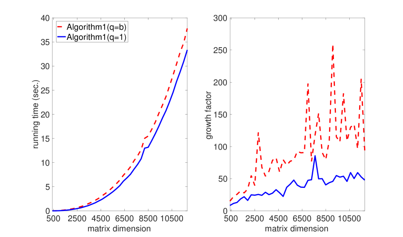
In Figure 5, we compare the efficiency difference between q=1𝑞1q=1 and q=b𝑞𝑏q=b on random matrices (Type 666 in numerical experiments). It confirms our analysis above that q=1𝑞1q=1 is the better option. Hence in the numerical experiments (Section 5), we only use Algorithm 1 with q=1𝑞1q=1. Curious enough, the option q=1𝑞1q=1 also gives smaller element growth factors than option q=b𝑞𝑏q=b, perhaps due to the likely reason that finding one pivot each time is more reliable than finding b𝑏b pivots in each loop.

Refer to caption
Figure 5: run time and growth factor of Algorithm 1 with different q𝑞q

3.2 Operation counts

In this section, we count the leading costs for the RCP algorithm, Bunch-Kaufman algorithm, and Aasen’s algorithm. Here we just do analysis of the BLAS-2 versions of these algorithms, since same analysis results will also apply for the BLAS-3 versions. In practice, we only use the BLAS-3 versions since they are much more efficient than BLAS-2 versions in terms of communication costs.

The operation count of the RCP algorithm is described in Figure 6. The terms Mults, Divs, Adds and Comps stand for the number of multiplications, divisions, additions, and comparisons respectively for each step of the Algorithm 1 with b=q=1𝑏𝑞1b=q=1.

Table 1 gives flops upper bounds, for solving a symmetric n×n𝑛𝑛n\times n linear system of equations, by the RCP algorithm, Bunch-Kaufman algorithm, and Aasen’s algorithm. All three algorithms are dominated by the same 13n313superscript𝑛3{\displaystyle\frac{1}{3}n^{3}} multiplication and addition costs. Aasen’s algorithm requires the fewest number of comparisons since it performs one column pivot per elimination step, whereas both the RCP and the Bunch-Kaufman algorithm perform up to two column pivots. Compared with the Bunch-Kaufman algorithm and Aasen’s algorithm, the RCP algorithm performs additional (2p12)n22𝑝12superscript𝑛2(2p-\frac{1}{2})n^{2} multiplications and additions. We choose p=5𝑝5p=5 in the numerical experiments, so the additional work is 9.5n29.5superscript𝑛29.5n^{2} flops, which is relatively insignificant for large n𝑛n. In Section 5, the results of our numerical experiments match this analysis.

Find πksubscript𝜋𝑘\pi_{k}.{Comps=nkMults, Adds=p(nk)casesComps𝑛𝑘Mults, Adds𝑝𝑛𝑘\left\{\begin{array}[]{l}\textrm{Comps}=n-k\\ \textrm{Mults, Adds}=p\,(n-k)\\ \end{array}\right.InterchangeFind λ𝜆\lambda.|a11|αλsubscript𝑎11𝛼𝜆\left|a_{11}\right|\geq\alpha\lambda?|arr|αλsubscript𝑎𝑟𝑟𝛼𝜆\left|a_{rr}\right|\geq\alpha\lambda?InterchangeUse 1×1111\times 1Calculate MultipliersDivs = nk𝑛𝑘n-kForm A(k+1)superscript𝐴𝑘1A^{(k+1)}{Multis, Adds=(nk)2/2casesMultis, Addsabsentsuperscript𝑛𝑘22\left\{\begin{array}[]{l}\textrm{Multis, Adds}=\\ (n-k)^{2}/2\end{array}\right.Update B(:,k+1:n)B(:,k+1:n){Mults, Adds=p(nk)casesMults, Addsabsent𝑝𝑛𝑘\left\{\begin{array}[]{l}\textrm{Mults, Adds}=\\ p\,(n-k)\end{array}\right.k=k+1𝑘𝑘1k=k+1InterchangeUse 2×2222\times 2Calculate DeterminantCalculate Multipliers{Mults=4(nk)Adds, Divs=2(nk)casesMults4𝑛𝑘Adds, Divs2𝑛𝑘\left\{\begin{array}[]{l}\textrm{Mults}=4\,(n-k)\\ \textrm{Adds, Divs}=2\,(n-k)\end{array}\right.Form A(k+2)superscript𝐴𝑘2A^{(k+2)}{Multis, Adds=(nk)2casesMultis, Addsabsentsuperscript𝑛𝑘2\left\{\begin{array}[]{l}\textrm{Multis, Adds}=\\ (n-k)^{2}\end{array}\right.Update B(:,k+2:n)B(:,k+2:n){Mults, Adds=2p(nk)casesMults, Addsabsent2𝑝𝑛𝑘\left\{\begin{array}[]{l}\textrm{Mults, Adds}=\\ 2\,p\,(n-k)\end{array}\right.k=k+2𝑘𝑘2k=k+2NoYesYesNo
Figure 6: Flowchart of operation counts for computing A(k+s)superscript𝐴𝑘𝑠A^{(k+s)} in RCP, s=1𝑠1s=1 or 222
Table 1: Comparison of the upper bounds for the number of operations
Algorithm Mults and Divs Adds Comps
RCP
   decomposition 16n3+(p+1)n216superscript𝑛3𝑝1superscript𝑛2\frac{1}{6}n^{3}+(p+1)n^{2} 16n3+(p12)n216superscript𝑛3𝑝12superscript𝑛2\frac{1}{6}n^{3}+(p-\frac{1}{2})n^{2} n2superscript𝑛2n^{2}
   solution phase n2superscript𝑛2n^{2} n2superscript𝑛2n^{2} 0
   total 16n3+(p+2)n216superscript𝑛3𝑝2superscript𝑛2\frac{1}{6}n^{3}+(p+2)n^{2} 16n3+(p+12)n216superscript𝑛3𝑝12superscript𝑛2\frac{1}{6}n^{3}+(p+\frac{1}{2})n^{2} n2superscript𝑛2n^{2}
Bunch-Kaufman
   decomposition 16n3+34n216superscript𝑛334superscript𝑛2\frac{1}{6}n^{3}+\frac{3}{4}n^{2} 16n3+14n216superscript𝑛314superscript𝑛2\frac{1}{6}n^{3}+\frac{1}{4}n^{2} n2superscript𝑛2n^{2}
   solution phase n2superscript𝑛2n^{2} n2superscript𝑛2n^{2} 0
   total 16n3+74n216superscript𝑛374superscript𝑛2\frac{1}{6}n^{3}+\frac{7}{4}n^{2} 16n3+54n216superscript𝑛354superscript𝑛2\frac{1}{6}n^{3}+\frac{5}{4}n^{2} n2superscript𝑛2n^{2}
Aasen
   decomposition 16n3+2n216superscript𝑛32superscript𝑛2\frac{1}{6}n^{3}+2n^{2} 16n3+n216superscript𝑛3superscript𝑛2\frac{1}{6}n^{3}+n^{2} 12n212superscript𝑛2\frac{1}{2}n^{2}
   solution phase n2superscript𝑛2n^{2} n2superscript𝑛2n^{2} n
   total 16n3+3n216superscript𝑛33superscript𝑛2\frac{1}{6}n^{3}+3n^{2} 16n3+2n216superscript𝑛32superscript𝑛2\frac{1}{6}n^{3}+2n^{2} 12n212superscript𝑛2\frac{1}{2}n^{2}

4 Analysis of randomized complete pivoting algorithm

To demonstrate its numerical reliability, in this section, we develop probabilistic upper bounds on both entries of the lower triangular matrix L𝐿L and on the element growth factor for the RCP algorithm. These upper bounds are much stronger than those for the Bunch-Kaufman algorithm. As the success of the RCP algorithm also depends on the numerical reliability of the random projections, we will study their numerical stability issues as well.

4.1 Reliability of randomized column pivots

The RCP algorithm chooses column pivots using norm-based column selections on the correlated random projections. Lemma 4.1 below justifies the reliability of these pivots and is the basis of much of our analysis on the RCP algorithm. In order to prove Lemma 4.1, we first show that the random projections do satisfy the Johnson-Lindenstrauss Lemma in a conditional sense, and then remove the condition with the Law of Total Probabilities.

Lemma 4.1.

(Randomized Norm Preservation) Given An×n𝐴superscript𝑛𝑛A\in\mathbb{R}^{n\times n}, over-sampling parameter p>0𝑝0p>0, and 0<ϵ,δ<1formulae-sequence0italic-ϵ𝛿10<\epsilon,~{}\delta<1. Assume that for every k𝑘k for which the RCP algorithm performs a random projection, the random matrix Ω(k)superscriptΩ𝑘\Omega^{(k)} is chosen as in equation (3) and let πk=𝐚𝐫𝐠𝐦𝐚𝐱kjnΩ(k)A(k)(:,j)2subscript𝜋𝑘subscript𝐚𝐫𝐠𝐦𝐚𝐱𝑘𝑗𝑛subscriptnormsuperscriptΩ𝑘superscript𝐴𝑘:𝑗2\pi_{k}={\bf argmax}_{k\leq j\leq n}\left\|\Omega^{(k)}A^{(k)}(:,j)\right\|_{2} be the column pivot. Then

(A(k)(:,πk)21ϵ1+ϵA(k)1,2)1δsubscriptnormsuperscript𝐴𝑘:subscript𝜋𝑘21italic-ϵ1italic-ϵsubscriptnormsuperscript𝐴𝑘121𝛿\mathbb{P}\left(\left\|A^{(k)}(:,\pi_{k})\right\|_{2}\geq\sqrt{\frac{1-\epsilon}{1+\epsilon}}\,\left\|A^{(k)}\right\|_{1,2}\right)\geq 1-\delta (5)

holds for all such k𝑘k, provided that p4ϵ2ϵ3ln(n(n+1)δ)𝑝4superscriptitalic-ϵ2superscriptitalic-ϵ3𝑛𝑛1𝛿p\geq\frac{4}{\epsilon^{2}-\epsilon^{3}}\ln{\left(\frac{n(n+1)}{\delta}\right)}.

Proof.

The diagonal permutation RCP chooses in the LDLT𝐿𝐷superscript𝐿𝑇LDL^{T} factorization is a discrete random variable. There are two parts in the RCP pivoting scheme. At each step k𝑘k, RCP chooses a column pivot based on column selection in the random projection matrix, and then makes a deterministic symmetric pivot based on the SBKP strategy. The LDLT𝐿𝐷superscript𝐿𝑇LDL^{T} factorization is uniquely determined by the diagonal permutation ΠΠ\Pi and block-diagonal pattern ΔΔ\Delta, which indicates whether each diagonal entry in D𝐷D is a 1×1111\times 1 pivot or part of a 2×2222\times 2 pivot.

Each LDLT𝐿𝐷superscript𝐿𝑇LDL^{T} factorization process with RCP results in a diagonal permutation and block-diagonal pattern pair (Π,Δ)ΠΔ\left(\Pi,\Delta\right), with some matrix A𝐴A dependent probability (Π,Δ)ΠΔ\mathbb{P}\left(\Pi,\Delta\right). It is clear that these (Π,Δ)ΠΔ\left(\Pi,\Delta\right) pairs are mutually exclusive and satisfy

(Π,Δ)(Π,Δ)=1.subscriptΠΔΠΔ1\sum_{\left(\Pi,\Delta\right)}\mathbb{P}\left(\Pi,\Delta\right)=1. (6)

Let Ωp×nΩsuperscript𝑝𝑛\Omega\in\mathbb{R}^{p\times n} be the I.I.D. Gaussian matrix drawn by RCP.

RCP begins its first column pivot with k=1𝑘1k=1. For 1jn1𝑗𝑛1\leq j\leq n, we denote the event that A(:,j)𝐴:𝑗A(:,j) satisfies ϵitalic-ϵ\epsilon-JL condition by E1,jsubscript𝐸1𝑗E_{1,j}. Thus

E1=def1jnE1,jsuperscript𝑑𝑒𝑓subscript𝐸1subscript1𝑗𝑛subscript𝐸1𝑗E_{1}\stackrel{{\scriptstyle def}}{{=}}\bigcap_{1\leq j\leq n}E_{1,j} (7)

is the event where every column of A(1)=Asuperscript𝐴1𝐴A^{(1)}=A satisfies the ϵitalic-ϵ\epsilon-JL condition under the random matrix ΩΩ\Omega. For any diagonal permutation ΠΠ\Pi and block-diagonal pattern pair (Π,Δ)ΠΔ\left(\Pi,\Delta\right), the column pivot π1subscript𝜋1\pi_{1} in the conditional event E1|(Π,Δ)conditionalsubscript𝐸1ΠΔE_{1}\left|\right.\left(\Pi,\Delta\right) must satisfy for any 1jn1𝑗𝑛1\leq j\leq n,

1ϵA(1)(:,j)21pB(:,j)21pB(:,π1)21+ϵA(1)(:,π1)2,1italic-ϵsubscriptnormsuperscript𝐴1:𝑗2subscriptnorm1𝑝𝐵:𝑗2subscriptnorm1𝑝𝐵:subscript𝜋121italic-ϵsubscriptnormsuperscript𝐴1:subscript𝜋12\sqrt{1-\epsilon}\left\|A^{(1)}(:,j)\right\|_{2}\leq\left\|\frac{1}{\sqrt{p}}B(:,j)\right\|_{2}\leq\left\|\frac{1}{\sqrt{p}}B(:,\pi_{1})\right\|_{2}\leq\sqrt{1+\epsilon}\left\|A^{(1)}(:,\pi_{1})\right\|_{2}, (8)

which implies

A(1)(:,π1)21ϵ1+ϵA(1)1,2.subscriptnormsuperscript𝐴1:subscript𝜋121italic-ϵ1italic-ϵsubscriptnormsuperscript𝐴112\left\|A^{(1)}(:,\pi_{1})\right\|_{2}\geq\sqrt{\frac{1-\epsilon}{1+\epsilon}}\,\left\|A^{(1)}\right\|_{1,2}. (9)

Under the diagonal permutation and block-diagonal pattern pair (Π,Δ)ΠΔ\left(\Pi,\Delta\right), we further assume that RCP performs a random projection at k𝑘k-th elimination step under (Π,Δ)ΠΔ\left(\Pi,\Delta\right) for some k𝑘k. Partition ΩΩ\Omega as in equation (3). It is clear that Ω~2subscript~Ω2\widetilde{\Omega}_{2} (the last ns𝑛𝑠n-s rows of Ω~~Ω\widetilde{\Omega}) is an I.I.D. Gaussian matrix conditioned under permutation ΠΠ\Pi.

Let A(k)superscript𝐴𝑘A^{(k)} be the Schur Complement. As with the case k=1𝑘1k=1, we denote the event that A(k)(:,j)superscript𝐴𝑘:𝑗A^{(k)}(:,j) satisfies ϵitalic-ϵ\epsilon-JL condition by Ek,jsubscript𝐸𝑘𝑗E_{k,j}, and let

Ek=defkjnEk,jsuperscript𝑑𝑒𝑓subscript𝐸𝑘subscript𝑘𝑗𝑛subscript𝐸𝑘𝑗E_{k}\stackrel{{\scriptstyle def}}{{=}}\bigcap_{k\leq j\leq n}E_{k,j} (10)

be the event that all columns of A(k)superscript𝐴𝑘A^{(k)} satisfy the ϵitalic-ϵ\epsilon-JL condition. As in Equation (9), the column pivot πksubscript𝜋𝑘\pi_{k} in the conditional event Ek|(Π,Δ)conditionalsubscript𝐸𝑘ΠΔE_{k}\left|\right.\left(\Pi,\Delta\right) must satisfy the condition

A(k)(:,πk)21ϵ1+ϵA(k)1,2.subscriptnormsuperscript𝐴𝑘:subscript𝜋𝑘21italic-ϵ1italic-ϵsubscriptnormsuperscript𝐴𝑘12\left\|A^{(k)}(:,\pi_{k})\right\|_{2}\geq\sqrt{\frac{1-\epsilon}{1+\epsilon}}\,\left\|A^{(k)}\right\|_{1,2}. (11)

In case RCP does not perform a random projection at k𝑘k-th elimination step, we define Ek,jsubscript𝐸𝑘𝑗E_{k,j} and Eksubscript𝐸𝑘E_{k} to be identically true events with (Ek,j)=(Ek)=1subscript𝐸𝑘𝑗subscript𝐸𝑘1\mathbb{P}\left(E_{k,j}\right)=\mathbb{P}\left(E_{k}\right)=1.

To develop a lower bound on the probability (Ek)subscript𝐸𝑘\mathbb{P}(E_{k}), we appeal to Law of Total Probability (Theorem 2.2),

(Ek)=(Π,Δ)(Ek|(Π,Δ))(Π,Δ),subscript𝐸𝑘subscriptΠΔconditionalsubscript𝐸𝑘ΠΔΠΔ\mathbb{P}(E_{k})=\sum_{\left(\Pi,\Delta\right)}\mathbb{P}\left(E_{k}\left|\right.\left(\Pi,\Delta\right)\right)\mathbb{P}\left(\Pi,\Delta\right),

where the sum is over all possible permutation and block-diagonal pattern pairs. By the Johnson-Lindenstrauss Lemma (Lemma 2.1),

(Ek|(Π,Δ))conditionalsubscript𝐸𝑘ΠΔ\displaystyle\mathbb{P}\left(E_{k}\left|\right.\left(\Pi,\Delta\right)\right) =(kjnEk,j|(Π,Δ))j=kn(Ek,j|(Π,Δ))(nk)absentconditionalsubscript𝑘𝑗𝑛subscript𝐸𝑘𝑗ΠΔsuperscriptsubscript𝑗𝑘𝑛conditionalsubscript𝐸𝑘𝑗ΠΔ𝑛𝑘\displaystyle=\mathbb{P}\left(\bigcap_{k\leq j\leq n}E_{k,j}\left|\right.\left(\Pi,\Delta\right)\right)\geq\sum_{j=k}^{n}\mathbb{P}\left(E_{k,j}|\left(\Pi,\Delta\right)\right)-(n-k)
j=kn(12exp((ϵ2ϵ3)p4))(nk)absentsuperscriptsubscript𝑗𝑘𝑛12superscriptitalic-ϵ2superscriptitalic-ϵ3𝑝4𝑛𝑘\displaystyle\geq\sum_{j=k}^{n}\left(1-2\exp\left(-\frac{(\epsilon^{2}-\epsilon^{3})p}{4}\right)\right)-(n-k)
=12(nk+1)exp((ϵ2ϵ3)p4).absent12𝑛𝑘1superscriptitalic-ϵ2superscriptitalic-ϵ3𝑝4\displaystyle=1-2(n-k+1)\exp\left(-\frac{(\epsilon^{2}-\epsilon^{3})p}{4}\right).

It now follows from Equation (6) that

(Ek)subscript𝐸𝑘\displaystyle\mathbb{P}(E_{k}) (12(nk+1)exp((ϵ2ϵ3)p4))(Π,Δ)(Π,Δ)absent12𝑛𝑘1superscriptitalic-ϵ2superscriptitalic-ϵ3𝑝4subscriptΠΔΠΔ\displaystyle\geq\left(1-2(n-k+1)\exp\left(-\frac{(\epsilon^{2}-\epsilon^{3})p}{4}\right)\right)\sum_{\left(\Pi,\Delta\right)}\mathbb{P}\left(\Pi,\Delta\right)
=12(nk+1)exp((ϵ2ϵ3)p4).absent12𝑛𝑘1superscriptitalic-ϵ2superscriptitalic-ϵ3𝑝4\displaystyle=1-2(n-k+1)\exp\left(-\frac{(\epsilon^{2}-\epsilon^{3})p}{4}\right).

Thus, for large enough p𝑝p, the norm of the pivot column chosen by RCP is a factor of 1ϵ1+ϵ1italic-ϵ1italic-ϵ{\displaystyle\sqrt{\frac{1-\epsilon}{1+\epsilon}}} away from optimal for any given k𝑘k with high probability.

To demonstrate that RCP chooses all such pivot columns with high probability, we let

E=def1knEksuperscript𝑑𝑒𝑓𝐸subscript1𝑘𝑛subscript𝐸𝑘{\displaystyle E\stackrel{{\scriptstyle def}}{{=}}\bigcap_{1\leq k\leq n}E_{k}}

to be the event that all the column pivots chosen by RCP satisfy the ϵitalic-ϵ\epsilon-JL condition. It follows that

(E)𝐸\displaystyle\mathbb{P}\left(E\right) =(k=1nEk)k=1n(Ek)(n1)absentsuperscriptsubscript𝑘1𝑛subscript𝐸𝑘superscriptsubscript𝑘1𝑛subscript𝐸𝑘𝑛1\displaystyle=\mathbb{P}\left(\bigcap_{k=1}^{n}E_{k}\right)\geq\sum_{k=1}^{n}\mathbb{P}(E_{k})-(n-1)
k=1n(12(nk+1)exp((ϵ2ϵ3)p4))(n1)absentsuperscriptsubscript𝑘1𝑛12𝑛𝑘1superscriptitalic-ϵ2superscriptitalic-ϵ3𝑝4𝑛1\displaystyle\geq\sum_{k=1}^{n}\left(1-2(n-k+1)\exp\left(-\frac{(\epsilon^{2}-\epsilon^{3})p}{4}\right)\right)-(n-1)
1n(n+1)exp((ϵ2ϵ3)p4),absent1𝑛𝑛1superscriptitalic-ϵ2superscriptitalic-ϵ3𝑝4\displaystyle\geq 1-n(n+1)\exp\left(-\frac{(\epsilon^{2}-\epsilon^{3})p}{4}\right),

the last expression is bounded below by 1δ1𝛿1-\delta for p4ϵ2ϵ3ln(n(n+1)δ)𝑝4superscriptitalic-ϵ2superscriptitalic-ϵ3𝑛𝑛1𝛿p\geq\frac{4}{\epsilon^{2}-\epsilon^{3}}\ln{\left(\frac{n(n+1)}{\delta}\right)}. ∎

Lemma 4.1 suggests that p𝑝p needs only to grow logarithmically with n𝑛n and 1/δ1𝛿1/\delta for reliable pivots. For illustration, if we choose n=1000,ϵ=0.5,δ=0.05formulae-sequence𝑛1000formulae-sequenceitalic-ϵ0.5𝛿0.05n=1000,\epsilon=0.5,\delta=0.05, then p538𝑝538p\geq 538. However, in practice, p𝑝p value like 555 suffices for RCP to obtain reliable pivots and hence reliable block LDLT𝐿𝐷superscript𝐿𝑇LDL^{T} factorization.

4.2 Upper Bounds on entries of the L matrix

In addition to potentially exponential element growth, the Bunch-Kaufman algorithm can also become numerically unstable due to potentially unbounded entries in the computed L𝐿L matrix [24]. In contrast, the entries in the L𝐿L matrix are upper bounded by O(1)𝑂1O(1) with symmetric complete pivoting [14]. In this section, we show that, with high probability, the entries of the matrix L𝐿L are upper bounded by O(n)𝑂𝑛O\left(\sqrt{n}\right) with the RCP algorithm, thus avoiding the potential numerical instability caused by unbounded L𝐿L entries.

Theorem 4.1.

Given An×n𝐴superscript𝑛𝑛A\in\mathbb{R}^{n\times n}, 0<ϵ,δ<1formulae-sequence0italic-ϵ𝛿10<\epsilon,~{}\delta<1, and over-sampling parameter

p4ϵ2ϵ3ln(n(n+1)δ),𝑝4superscriptitalic-ϵ2superscriptitalic-ϵ3𝑛𝑛1𝛿{\displaystyle p\geq\frac{4}{\epsilon^{2}-\epsilon^{3}}\ln{\left(\frac{n(n+1)}{\delta}\right)},}

then with probability at least 1δ1𝛿1-\delta,

|li,k|1+1+ϵ1ϵnk+1𝐦𝐢𝐧(α,1α2)for all1k<in.formulae-sequencesubscript𝑙𝑖𝑘11italic-ϵ1italic-ϵ𝑛𝑘1𝐦𝐢𝐧𝛼1superscript𝛼2for all1𝑘𝑖𝑛{\displaystyle\left|l_{i,k}\right|\leq\frac{1+\sqrt{\frac{1+\epsilon}{1-\epsilon}}\,\sqrt{n-k+1}}{{\bf min}\left(\alpha,1-\alpha^{2}\right)}}\quad\mbox{for all}\quad 1\leq k<i\leq n. (12)
Proof.

There are three non-trivial cases when the SBKP strategy (Figure 4) is applied to the first column of matrix A=defA(1)superscript𝑑𝑒𝑓𝐴superscript𝐴1A\stackrel{{\scriptstyle def}}{{=}}A^{(1)} with k=1𝑘1k=1, resulting in an s×s𝑠𝑠s\times s pivoting block with s=1𝑠1s=1 or 222. The SBKP strategy will then proceed to perform subsequent eliminations on the Schur complement A(1+s)=def(aij(1+s))i,j=k+snsuperscript𝑑𝑒𝑓superscript𝐴1𝑠superscriptsubscriptsuperscriptsubscript𝑎𝑖𝑗1𝑠𝑖𝑗𝑘𝑠𝑛A^{(1+s)}\stackrel{{\scriptstyle def}}{{=}}\left(a_{ij}^{(1+s)}\right)_{i,j=k+s}^{n}. Below we consider each case.

Case (1):

a1,1subscript𝑎11a_{1,1} is the 1×1111\times 1 pivot with |a1,1|αλsubscript𝑎11𝛼𝜆\left|a_{1,1}\right|\geq\alpha\lambda, where λ=𝐦𝐚𝐱2jn|aj,1|𝜆subscript𝐦𝐚𝐱2𝑗𝑛subscript𝑎𝑗1\lambda={\bf max}_{2\leq j\leq n}\left|a_{j,1}\right|. In this case,

lj,1subscript𝑙𝑗1\displaystyle l_{j,1} =aj,1/a1,1,forj>1,formulae-sequenceabsentsubscript𝑎𝑗1subscript𝑎11for𝑗1\displaystyle=a_{j,1}/a_{1,1},\quad\mbox{for}\quad j>1,
and therefore|lj,1|and thereforesubscript𝑙𝑗1\displaystyle\mbox{and therefore}\quad\left|l_{j,1}\right| 1α,absent1𝛼\displaystyle\leq\frac{1}{\alpha},

which obviously satisfies equation (12).

Case (2):

ar,rsubscript𝑎𝑟𝑟a_{r,r} is the 1×1111\times 1 pivot with |arr|αλsubscript𝑎𝑟𝑟𝛼𝜆\left|a_{rr}\right|\geq\alpha\lambda. After the row and column interchanges, we have

lj,1={aj,r/ar,r,for2jn,jr,a1,r/ar,r,forj=r.subscript𝑙𝑗1casessubscript𝑎𝑗𝑟subscript𝑎𝑟𝑟formulae-sequencefor2𝑗𝑛𝑗𝑟subscript𝑎1𝑟subscript𝑎𝑟𝑟for𝑗𝑟l_{j,1}=\left\{\begin{array}[]{ll}a_{j,r}/a_{r,r},&\mbox{for}\quad 2\leq j\leq n,~{}j\not=r,\\ a_{1,r}/a_{r,r},&\mbox{for}\quad j=r.\end{array}\right. (13)

For any jr𝑗𝑟j\neq r, it follows from Lemma 4.1 that

|aj,r|A(:,r)21+ϵ1ϵA(:,1)21+ϵ1ϵλn.subscript𝑎𝑗𝑟subscriptnorm𝐴:𝑟21italic-ϵ1italic-ϵsubscriptnorm𝐴:121italic-ϵ1italic-ϵ𝜆𝑛|a_{j,r}|\leq\left\|A(:,r)\right\|_{2}\leq\sqrt{\frac{1+\epsilon}{1-\epsilon}}\,\left\|A(:,1)\right\|_{2}\leq\sqrt{\frac{1+\epsilon}{1-\epsilon}}\,\lambda\,\sqrt{n}.

Plugging this into equation (13) yields

|lj,1|1+ϵ1ϵnα,subscript𝑙𝑗11italic-ϵ1italic-ϵ𝑛𝛼{\displaystyle\left|l_{j,1}\right|\leq\frac{\sqrt{\frac{1+\epsilon}{1-\epsilon}}\,\sqrt{n}}{\alpha}},

which satisfies equation (12) with k=1𝑘1k=1.

Case (3):

The SBKP strategy chooses a 2×2222\times 2 pivot (a1,1ar,1ar,1ar,r)subscript𝑎11subscript𝑎𝑟1subscript𝑎𝑟1subscript𝑎𝑟𝑟\left(\begin{array}[]{cc}a_{1,1}&a_{r,1}\\ a_{r,1}&a_{r,r}\end{array}\right) with s=2𝑠2s=2. After the row and column interchanges, we have that for any j3𝑗3j\geq 3, let

i={j,for3jn,jr,2,forj=r.𝑖cases𝑗formulae-sequencefor3𝑗𝑛𝑗𝑟2for𝑗𝑟i=\left\{\begin{array}[]{ll}j,&\mbox{for}\quad 3\leq j\leq n,~{}j\not=r,\\ 2,&\mbox{for}\quad j=r.\end{array}\right.

Then

(lj,1,lj,2)subscript𝑙𝑗1subscript𝑙𝑗2\displaystyle\left(l_{j,1},\;\;l_{j,2}\right) =(ai,1,ai,r)(a1,1ar,1ar,1ar,r)1absentsubscript𝑎𝑖1subscript𝑎𝑖𝑟superscriptsubscript𝑎11subscript𝑎𝑟1subscript𝑎𝑟1subscript𝑎𝑟𝑟1\displaystyle=\left(a_{i,1},\;\;a_{i,r}\right)\left(\begin{array}[]{cc}a_{1,1}&a_{r,1}\\ a_{r,1}&a_{r,r}\end{array}\right)^{-1}
=1a1,1ar,rar,12(ai,1ar,rar,1ai,r,a1,1ai,rar,1ai,1).absent1subscript𝑎11subscript𝑎𝑟𝑟superscriptsubscript𝑎𝑟12subscript𝑎𝑖1subscript𝑎𝑟𝑟subscript𝑎𝑟1subscript𝑎𝑖𝑟subscript𝑎11subscript𝑎𝑖𝑟subscript𝑎𝑟1subscript𝑎𝑖1\displaystyle=\frac{1}{a_{1,1}\,a_{r,r}-a_{r,1}^{2}}\left(a_{i,1}\,a_{r,r}-a_{r,1}\,a_{i,r},\;\;a_{1,1}\,a_{i,r}-a_{r,1}\,a_{i,1}\right).

Since |a1,1|<αλsubscript𝑎11𝛼𝜆|a_{1,1}|<\alpha\lambda, |ar,r|<αλsubscript𝑎𝑟𝑟𝛼𝜆|a_{r,r}|<\alpha\lambda, and

|ai,r|1+ϵ1ϵλn,subscript𝑎𝑖𝑟1italic-ϵ1italic-ϵ𝜆𝑛|a_{i,r}|\leq\sqrt{\frac{1+\epsilon}{1-\epsilon}}\,\lambda\,\sqrt{n},

we deduce that

|lj,1|,|lj,2|λ2+1+ϵ1ϵλ2nλ2(1α2)=1+1+ϵ1ϵn1α2,subscript𝑙𝑗1subscript𝑙𝑗2superscript𝜆21italic-ϵ1italic-ϵsuperscript𝜆2𝑛superscript𝜆21superscript𝛼211italic-ϵ1italic-ϵ𝑛1superscript𝛼2|l_{j,1}|,\;\;|l_{j,2}|\leq\frac{\lambda^{2}+\sqrt{\frac{1+\epsilon}{1-\epsilon}}\,\lambda^{2}\,\sqrt{n}}{\lambda^{2}\,(1-\alpha^{2})}=\frac{1+\sqrt{\frac{1+\epsilon}{1-\epsilon}}\,\sqrt{n}}{1-\alpha^{2}},

which again satisfies equation (12) with k=1𝑘1k=1.

To complete the proof for Theorem 4.1, we recursively apply the same argument above to the Schur complement A(k)superscript𝐴𝑘A^{(k)} in each case, taking note that the dimension of A(k)superscript𝐴𝑘A^{(k)} for any k𝑘k is nk+1𝑛𝑘1n-k+1. ∎

In next section, we will show that we can also deduce a much better column growth factor bound using Wilkinson’s techniques for GECP [38]. His proof is dependent on the fact that the pivots in GECP are maximum elements in the Schur complement. Our pivots are not necessarily maximum elements, but they are closely related to the maximum column norm in the Schur complement. Thus, we need more subtle analysis.

4.3 Probability analysis on column growth factor

In this section, we present a rigorous upper bound on the column norm growth factor of LDLT𝐿𝐷superscript𝐿𝑇LDL^{T} factorization computed by the RCP algorithm.

Theorem 4.2.

(Column Growth Factor for Randomized Complete Pivoting).
Given An×n𝐴superscript𝑛𝑛A\in\mathbb{R}^{n\times n}, 0<ϵ,δ<1formulae-sequence0italic-ϵ𝛿10<\epsilon,~{}\delta<1, and over-sampling parameter

p4ϵ2ϵ3ln(n(n+1)δ),𝑝4superscriptitalic-ϵ2superscriptitalic-ϵ3𝑛𝑛1𝛿{\displaystyle p\geq\frac{4}{\epsilon^{2}-\epsilon^{3}}\ln{\left(\frac{n(n+1)}{\delta}\right)},}

then the column norm growth factor of RCP algorithm, with α=22𝛼22\alpha=\frac{\sqrt{2}}{2} in the SBKP strategy, satisfies

ρcol(2(1+ϵ)1ϵ)3+ln(n1)(n+2)2+ln(n1)subscript𝜌colsuperscript21italic-ϵ1italic-ϵ3𝑛1superscript𝑛22𝑛1\rho_{\textrm{col}}\leq\left(\sqrt{\frac{2(1+\epsilon)}{1-\epsilon}}\right)^{3+\ln(n-1)}\,\left(\sqrt{n+2}\right)^{2+\ln(n-1)}

with probability at least 1δ1𝛿1-\delta.

Proof.

Following Wilkinson [38], our approach is to establish a recursive relationship among the diagonal entries of the D𝐷D matrix using the Hadamard’s inequality (Theorem 2.1). The upper bound on ρcolsubscript𝜌col\rho_{\textrm{col}} is then obtained by solving this recursion.

Similar to the element growth factor analysis for Bunch-Parlett algorithm [12], we adopt the following notation:

pivot[k]=def{1, 1×1pivotinA(k),(|akk(k)|αλ(k)or|arr(k)|αλ(k)>|akk(k)|),2, 2×2pivotinA(k),(|akk(k)|,|arr(k)|<αλ(k)),0, 2×2pivotinA(k1),(|ak1,k1(k1)|,|arr(k1)|<αλ(k1)).superscript𝑑𝑒𝑓𝑝𝑖𝑣𝑜𝑡delimited-[]𝑘cases111pivotinsuperscript𝐴𝑘superscriptsubscript𝑎𝑘𝑘𝑘𝛼superscript𝜆𝑘orsuperscriptsubscript𝑎𝑟𝑟𝑘𝛼superscript𝜆𝑘superscriptsubscript𝑎𝑘𝑘𝑘missing-subexpressionmissing-subexpressionmissing-subexpressionmissing-subexpressionmissing-subexpression222pivotinsuperscript𝐴𝑘superscriptsubscript𝑎𝑘𝑘𝑘superscriptsubscript𝑎𝑟𝑟𝑘𝛼superscript𝜆𝑘missing-subexpressionmissing-subexpressionmissing-subexpressionmissing-subexpressionmissing-subexpression022pivotinsuperscript𝐴𝑘1superscriptsubscript𝑎𝑘1𝑘1𝑘1superscriptsubscript𝑎𝑟𝑟𝑘1𝛼superscript𝜆𝑘1missing-subexpressionmissing-subexpressionpivot[k]\stackrel{{\scriptstyle def}}{{=}}\left\{\begin{array}[]{lll}1,\>1\times 1~{}\mbox{pivot}~{}\mbox{in}~{}A^{(k)},\left(~{}\left|a_{kk}^{(k)}\right|\geq\alpha\,\lambda^{(k)}~{}\mbox{or}~{}\left|a_{rr}^{(k)}\right|\geq\alpha\,\lambda^{(k)}>\left|a_{kk}^{(k)}\right|\right),\\ \\ 2,\>2\times 2~{}\mbox{pivot}~{}\mbox{in}~{}A^{(k)},\left(~{}\left|a_{kk}^{(k)}\right|,\left|a_{rr}^{(k)}\right|<\alpha\,\lambda^{(k)}\right),\\ \\ 0,\>2\times 2~{}\mbox{pivot}~{}\mbox{in}~{}A^{(k-1)},\left(~{}\left|a_{k-1,k-1}^{(k-1)}\right|,\left|a_{rr}^{(k-1)}\right|<\alpha\,\lambda^{(k-1)}\right).\end{array}\right.
v(k)=def|det(akk(k)ark(k)ark(k)arr(k))|=|akk(k)arr(k)(ark(k))2|.superscript𝑑𝑒𝑓superscript𝑣𝑘superscriptsubscript𝑎𝑘𝑘𝑘superscriptsubscript𝑎𝑟𝑘𝑘superscriptsubscript𝑎𝑟𝑘𝑘superscriptsubscript𝑎𝑟𝑟𝑘superscriptsubscript𝑎𝑘𝑘𝑘superscriptsubscript𝑎𝑟𝑟𝑘superscriptsuperscriptsubscript𝑎𝑟𝑘𝑘2v^{(k)}\stackrel{{\scriptstyle def}}{{=}}\left|\det\left(\begin{array}[]{cc}a_{kk}^{(k)}&a_{rk}^{(k)}\\ a_{rk}^{(k)}&a_{rr}^{(k)}\end{array}\right)\right|=\left|a_{kk}^{(k)}\,a_{rr}^{(k)}-\left(a_{rk}^{(k)}\right)^{2}\right|.
pk=def{|akk(k)| or |arr(k)|if pivot[k]=1,v(k)if pivot[k]=2,v(k1)if pivot[k]=0.superscript𝑑𝑒𝑓subscript𝑝𝑘cases|akk(k)| or |arr(k)|if pivot[k]=1,superscript𝑣𝑘if pivot[k]=2,superscript𝑣𝑘1if pivot[k]=0.p_{k}\stackrel{{\scriptstyle def}}{{=}}\left\{\begin{array}[]{ll}\mbox{$\left|a_{kk}^{(k)}\right|$ or $\left|a_{rr}^{(k)}\right|$}&\mbox{if $pivot[k]=1,$}\\ \sqrt{v^{(k)}}&\mbox{if $pivot[k]=2,$}\\ \sqrt{v^{(k-1)}}&\mbox{if $pivot[k]=0.$}\end{array}\right.

Therefore, for kmn𝑘𝑚𝑛k\leq m\leq n,

|det(A(k)(k:m,k:m))|=j=kmpj.\left|\det\left(A^{(k)}(k:m,k:m)\right)\right|=\prod_{j=k}^{m}p_{j}. (14)

Let ck=defA(k)(:,πk)2superscript𝑑𝑒𝑓subscript𝑐𝑘subscriptnormsuperscript𝐴𝑘:subscript𝜋𝑘2c_{k}\stackrel{{\scriptstyle def}}{{=}}\left\|A^{(k)}(:,\pi_{k})\right\|_{2} be the 2-norm of the pivot column of A(k)superscript𝐴𝑘A^{(k)}, where πk=𝐚𝐫𝐠𝐦𝐚𝐱kjnΩ(k)A(k)(:,j)2subscript𝜋𝑘subscript𝐚𝐫𝐠𝐦𝐚𝐱𝑘𝑗𝑛subscriptnormsuperscriptΩ𝑘superscript𝐴𝑘:𝑗2\pi_{k}={\bf argmax}_{k\leq j\leq n}\left\|\Omega^{(k)}A^{(k)}(:,j)\right\|_{2}. When pivot[k]=0𝑝𝑖𝑣𝑜𝑡delimited-[]𝑘0pivot[k]=0, ck=ck1subscript𝑐𝑘subscript𝑐𝑘1c_{k}=c_{k-1}. For each pivot possibility, we deduce a lower bound for pksubscript𝑝𝑘p_{k}.

Case (1): pivot[k]=1𝑝𝑖𝑣𝑜𝑡delimited-[]𝑘1pivot[k]=1.

pk𝐦𝐚𝐱{αλ(k),|akk(k)|}𝐦𝐚𝐱{αλ(k),α|akk(k)|}αnk+1ck,subscript𝑝𝑘𝐦𝐚𝐱𝛼superscript𝜆𝑘superscriptsubscript𝑎𝑘𝑘𝑘𝐦𝐚𝐱𝛼superscript𝜆𝑘𝛼superscriptsubscript𝑎𝑘𝑘𝑘𝛼𝑛𝑘1subscript𝑐𝑘p_{k}\geq{\bf max}\left\{\alpha\,\lambda^{(k)},\left|a_{kk}^{(k)}\right|\right\}\geq{\bf max}\left\{\alpha\,\lambda^{(k)},\alpha\,\left|a_{kk}^{(k)}\right|\right\}\geq\frac{\alpha}{\sqrt{n-k+1}}\,c_{k},

where the first inequality holds because of the definition of pksubscript𝑝𝑘p_{k} when pivot[k]=1𝑝𝑖𝑣𝑜𝑡delimited-[]𝑘1pivot[k]=1, and the second inequality holds because of the fact that 0<α<10𝛼10<\alpha<1, and the third inequality holds because of a simple property of the entry with the largest magnitude in the pivot column of A(k)superscript𝐴𝑘A^{(k)}.

Case (2): pivot[k]=2𝑝𝑖𝑣𝑜𝑡delimited-[]𝑘2pivot[k]=2.

pk=v(k)=|(ark(k))2akk(k)arr(k)|1α2λ(k)1α2nk+1ck.subscript𝑝𝑘superscript𝑣𝑘superscriptsuperscriptsubscript𝑎𝑟𝑘𝑘2superscriptsubscript𝑎𝑘𝑘𝑘superscriptsubscript𝑎𝑟𝑟𝑘1superscript𝛼2superscript𝜆𝑘1superscript𝛼2𝑛𝑘1subscript𝑐𝑘p_{k}=\sqrt{v^{(k)}}=\sqrt{\left|\left(a_{rk}^{(k)}\right)^{2}-a_{kk}^{(k)}\,a_{rr}^{(k)}\right|}\geq\sqrt{1-\alpha^{2}}\,\lambda^{(k)}\geq\frac{\sqrt{1-\alpha^{2}}}{\sqrt{n-k+1}}\,c_{k}.

where the first inequality holds because |ark(k)|=λ(k),|akk(k)|<αλ(k) and |arr(k)|<αλ(k).formulae-sequencesuperscriptsubscript𝑎𝑟𝑘𝑘superscript𝜆𝑘superscriptsubscript𝑎𝑘𝑘𝑘𝛼superscript𝜆𝑘 and superscriptsubscript𝑎𝑟𝑟𝑘𝛼superscript𝜆𝑘\left|a_{rk}^{(k)}\right|=\lambda^{(k)},\left|a_{kk}^{(k)}\right|<\alpha\,\lambda^{(k)}\mbox{ and }\left|a_{rr}^{(k)}\right|<\alpha\,\lambda^{(k)}.

Case (3): pivot[k]=0𝑝𝑖𝑣𝑜𝑡delimited-[]𝑘0pivot[k]=0.

pksubscript𝑝𝑘\displaystyle p_{k} =\displaystyle= v(k1)=|(ar,k1(k1))2ak1,k1(k1)arr(k1)|superscript𝑣𝑘1superscriptsuperscriptsubscript𝑎𝑟𝑘1𝑘12superscriptsubscript𝑎𝑘1𝑘1𝑘1superscriptsubscript𝑎𝑟𝑟𝑘1\displaystyle\sqrt{v^{(k-1)}}=\sqrt{\left|\left(a_{r,k-1}^{(k-1)}\right)^{2}-a_{k-1,k-1}^{(k-1)}a_{rr}^{(k-1)}\right|}
\displaystyle\geq 1α2nk+2ck1=1α2nk+2ck.1superscript𝛼2𝑛𝑘2subscript𝑐𝑘11superscript𝛼2𝑛𝑘2subscript𝑐𝑘\displaystyle\frac{\sqrt{1-\alpha^{2}}}{\sqrt{n-k+2}}c_{k-1}=\frac{\sqrt{1-\alpha^{2}}}{\sqrt{n-k+2}}c_{k}.

since |ar,k1(k1)|=λ(k1),|ak1,k1(k1)|<αλ(k1) and |arr(k1)|<αλ(k1).formulae-sequencesuperscriptsubscript𝑎𝑟𝑘1𝑘1superscript𝜆𝑘1superscriptsubscript𝑎𝑘1𝑘1𝑘1𝛼superscript𝜆𝑘1 and superscriptsubscript𝑎𝑟𝑟𝑘1𝛼superscript𝜆𝑘1\left|a_{r,k-1}^{(k-1)}\right|=\lambda^{(k-1)},\left|a_{k-1,k-1}^{(k-1)}\right|<\alpha\,\lambda^{(k-1)}\mbox{ and }\left|a_{rr}^{(k-1)}\right|<\alpha\,\lambda^{(k-1)}.

Let t(α)=def𝐦𝐢𝐧(α,1α2)superscript𝑑𝑒𝑓𝑡𝛼𝐦𝐢𝐧𝛼1superscript𝛼2t(\alpha)\stackrel{{\scriptstyle def}}{{=}}{\bf min}\left(\alpha,\;\sqrt{1-\alpha^{2}}\right), then all the above three cases deduce to

pkt(α)nk+2ck.subscript𝑝𝑘𝑡𝛼𝑛𝑘2subscript𝑐𝑘p_{k}\geq\frac{t(\alpha)}{\sqrt{n-k+2}}\,c_{k}.

From equation (14),

|det(A(k)(k:m,k:m))|j=kmt(α)nj+2cj=t(α)mk+1j=kmcjnj+2.\displaystyle\left|\det\left(A^{(k)}(k:m,k:m)\right)\right|\geq\prod_{j=k}^{m}\frac{t(\alpha)}{\sqrt{n-j+2}}\,c_{j}=t(\alpha)^{m-k+1}\,\prod_{j=k}^{m}\frac{c_{j}}{\sqrt{n-j+2}}. (15)

We can also obtain an upper bound of the determinant of A(k)(k:m,k:m)A^{(k)}(k:m,k:m) by applying Hadamard’s inequality (Theorem 2.1), that is

|det(A(k)(k:m,k:m))|\displaystyle\left|\det\left(A^{(k)}(k:m,k:m)\right)\right| j=kmA(k)(k:m,j)2j=kmA(k)(:,j)2\displaystyle\leq\prod_{j=k}^{m}\left\|A^{(k)}(k:m,j)\right\|_{2}\leq\prod_{j=k}^{m}\left\|A^{(k)}(:,j)\right\|_{2}
(1+ϵ1ϵ)mk+1A(k)(:,πk)2mk+1absentsuperscript1italic-ϵ1italic-ϵ𝑚𝑘1superscriptsubscriptnormsuperscript𝐴𝑘:subscript𝜋𝑘2𝑚𝑘1\displaystyle\leq\left(\sqrt{\frac{1+\epsilon}{1-\epsilon}}\right)^{m-k+1}\left\|A^{(k)}(:,\pi_{k})\right\|_{2}^{m-k+1}
=(1+ϵ1ϵ)mk+1ckmk+1,absentsuperscript1italic-ϵ1italic-ϵ𝑚𝑘1superscriptsubscript𝑐𝑘𝑚𝑘1\displaystyle=\left(\sqrt{\frac{1+\epsilon}{1-\epsilon}}\right)^{m-k+1}\,c_{k}^{m-k+1}, (16)

where the second inequality holds because the 222-norm of the j𝑗j-th column of the Schur complement A(k)superscript𝐴𝑘A^{(k)} is greater than or equal to the 222-norm of the first few entries of the j𝑗j-th column of the Schur complement A(k)superscript𝐴𝑘A^{(k)}. The third one holds because of Lemma 4.1. Combining inequalities (15) and (4.3) together for |det(A(k)(k:m,k:m))|\left|\det\left(A^{(k)}(k:m,k:m)\right)\right|, we obtain that

j=kmcjnj+2(1t(α)1+ϵ1ϵ)mk+1ckmk+1.superscriptsubscriptproduct𝑗𝑘𝑚subscript𝑐𝑗𝑛𝑗2superscript1𝑡𝛼1italic-ϵ1italic-ϵ𝑚𝑘1superscriptsubscript𝑐𝑘𝑚𝑘1\displaystyle\prod_{j=k}^{m}\frac{c_{j}}{\sqrt{n-j+2}}\leq\left(\frac{1}{t(\alpha)}\,\sqrt{\frac{1+\epsilon}{1-\epsilon}}\right)^{m-k+1}c_{k}^{m-k+1}.

For all 1kmn1𝑘𝑚𝑛1\leq k\leq m\leq n, we take logarithms on both sides and define

qj=defln(cj),superscript𝑑𝑒𝑓subscript𝑞𝑗subscript𝑐𝑗q_{j}\stackrel{{\scriptstyle def}}{{=}}\ln(c_{j}),

the above inequality becomes a linear recursive inequality,

j=k+1mqj(mk+1)ln(1t(α)1+ϵ1ϵ)+j=kmln(nj+2)+(mk)qk.superscriptsubscript𝑗𝑘1𝑚subscript𝑞𝑗𝑚𝑘11𝑡𝛼1italic-ϵ1italic-ϵsuperscriptsubscript𝑗𝑘𝑚𝑛𝑗2𝑚𝑘subscript𝑞𝑘\sum_{j=k+1}^{m}q_{j}\leq(m-k+1)\,\ln\left(\frac{1}{t(\alpha)}\,\sqrt{\frac{1+\epsilon}{1-\epsilon}}\right)+\sum_{j=k}^{m}\ln\left(\sqrt{n-j+2}\right)+(m-k)\,q_{k}.

Below we derive an upper bound on qmsubscript𝑞𝑚q_{m} by solving this recursion.

Dividing both sides by (mk)(mk+1)𝑚𝑘𝑚𝑘1(m-k)(m-k+1) for k=2,3,,m1𝑘23𝑚1k=2,3,\cdots,m-1, and by mk𝑚𝑘m-k for k=1𝑘1k=1 and adding all m1𝑚1m-1 equations, on observing that

1m1+1(m2)(m1)++1(mk)(mk+1)=1mk,1𝑚11𝑚2𝑚11𝑚𝑘𝑚𝑘11𝑚𝑘\frac{1}{m-1}+\frac{1}{(m-2)(m-1)}+\cdots+\frac{1}{(m-k)(m-k+1)}=\frac{1}{m-k},

we obtain

qmsubscript𝑞𝑚\displaystyle q_{m} \displaystyle\leq (1+j=1m11j)ln(1t(α)1+ϵ1ϵ)1superscriptsubscript𝑗1𝑚11𝑗1𝑡𝛼1italic-ϵ1italic-ϵ\displaystyle\left(1+\sum_{j=1}^{m-1}\frac{1}{j}\right)\ln\left(\frac{1}{t(\alpha)}\,\sqrt{\frac{1+\epsilon}{1-\epsilon}}\right) (17)
+ln(nm+2)+j=1m11jln(nm+2+j)+q1𝑛𝑚2superscriptsubscript𝑗1𝑚11𝑗𝑛𝑚2𝑗subscript𝑞1\displaystyle+\ln\left(\sqrt{n-m+2}\right)+\sum_{j=1}^{m-1}\frac{1}{j}\,\ln\left(\sqrt{n-m+2+j}\right)+q_{1}
\displaystyle\leq (1+j=1m11j)(ln(1t(α)1+ϵ1ϵ)+lnn+1)+ln(n+2)+q11superscriptsubscript𝑗1𝑚11𝑗1𝑡𝛼1italic-ϵ1italic-ϵ𝑛1𝑛2subscript𝑞1\displaystyle\left(1+\sum_{j=1}^{m-1}\frac{1}{j}\right)\left(\ln\left(\frac{1}{t(\alpha)}\,\sqrt{\frac{1+\epsilon}{1-\epsilon}}\right)+\ln\sqrt{n+1}\right)+\ln\left(\sqrt{n+2}\right)+q_{1}

Since

j=1m11j1+ln(m1),superscriptsubscript𝑗1𝑚11𝑗1𝑚1\sum_{j=1}^{m-1}\frac{1}{j}\leq 1+\ln(m-1), (18)

Plugging this into (17),

qmq1subscript𝑞𝑚subscript𝑞1\displaystyle q_{m}-q_{1} (2+ln(n1))(ln(1t(α)1+ϵ1ϵ)+lnn+1)+ln(n+2).absent2𝑛11𝑡𝛼1italic-ϵ1italic-ϵ𝑛1𝑛2\displaystyle\leq\left(2+\ln(n-1)\right)\left(\ln\left(\frac{1}{t(\alpha)}\,\sqrt{\frac{1+\epsilon}{1-\epsilon}}\right)+\ln\sqrt{n+1}\right)+\ln\left(\sqrt{n+2}\right).

The upper bound above holds true for all m𝑚m. Taking the exponential of both sides, for all 1mn1𝑚𝑛1\leq m\leq n,

cmc1n+2(1t(α)1+ϵ1ϵ)(2+ln(n1))(n+1)(2+ln(n1)).subscript𝑐𝑚subscript𝑐1𝑛2superscript1𝑡𝛼1italic-ϵ1italic-ϵ2𝑛1superscript𝑛12𝑛1\frac{c_{m}}{c_{1}}\leq\sqrt{n+2}\,\left(\frac{1}{t(\alpha)}\,\sqrt{\frac{1+\epsilon}{1-\epsilon}}\right)^{\left(2+\ln(n-1)\right)}\,\left(\sqrt{n+1}\right)^{\left(2+\ln(n-1)\right)}.

Now we estimate ρcolsubscript𝜌col\rho_{\textrm{col}} using cmc1subscript𝑐𝑚subscript𝑐1{\displaystyle\frac{c_{m}}{c_{1}}},

ρcolsubscript𝜌col\displaystyle\rho_{\textrm{col}} =𝐦𝐚𝐱mA(m)1,2A1,21+ϵ1ϵ𝐦𝐚𝐱mA(m)(:,πm)2A(1)(:,π1)2=1+ϵ1ϵ𝐦𝐚𝐱mcmc1absentsubscript𝐦𝐚𝐱𝑚subscriptnormsuperscript𝐴𝑚12subscriptnorm𝐴121italic-ϵ1italic-ϵsubscript𝐦𝐚𝐱𝑚subscriptnormsuperscript𝐴𝑚:subscript𝜋𝑚2subscriptnormsuperscript𝐴1:subscript𝜋121italic-ϵ1italic-ϵsubscript𝐦𝐚𝐱𝑚subscript𝑐𝑚subscript𝑐1\displaystyle=\frac{{\bf max}_{m}\left\|A^{(m)}\right\|_{1,2}}{\|A\|_{1,2}}\leq\sqrt{\frac{1+\epsilon}{1-\epsilon}}\,{\bf max}_{m}\frac{\left\|A^{(m)}(:,\pi_{m})\right\|_{2}}{\|A^{(1)}(:,\pi_{1})\|_{2}}=\sqrt{\frac{1+\epsilon}{1-\epsilon}}\,{\bf max}_{m}\frac{c_{m}}{c_{1}}
(1t(α)1+ϵ1ϵ)(3+ln(n1))(n+2)(2+ln(n1)).absentsuperscript1𝑡𝛼1italic-ϵ1italic-ϵ3𝑛1superscript𝑛22𝑛1\displaystyle\leq\left(\frac{1}{t(\alpha)}\,\sqrt{\frac{1+\epsilon}{1-\epsilon}}\right)^{\left(3+\ln(n-1)\right)}\,\left(\sqrt{n+2}\right)^{\left(2+\ln(n-1)\right)}. (19)

The function t(α)𝑡𝛼t(\alpha) achieves its maximum at α=22𝛼22\alpha=\frac{\sqrt{2}}{2}. With this choice of α𝛼\alpha, equation (4.3) becomes

ρcolsubscript𝜌col\displaystyle\rho_{\textrm{col}} (2(1+ϵ)1ϵ)(3+ln(n1))(n+2)(2+ln(n1)).absentsuperscript21italic-ϵ1italic-ϵ3𝑛1superscript𝑛22𝑛1\displaystyle\leq\left(\sqrt{\frac{2(1+\epsilon)}{1-\epsilon}}\right)^{\left(3+\ln(n-1)\right)}\,\left(\sqrt{n+2}\right)^{\left(2+\ln(n-1)\right)}. (20)

Corollary 4.1 below follows directly from Lemma 2.2 and Theorem 4.2.

Corollary 4.1.

(Element Growth Factor for Randomized Complete Pivoting). Under the assumptions of Theorem 4.2, the element growth factor of RCP algorithm, with α=22𝛼22\alpha=\frac{\sqrt{2}}{2} in the SBKP strategy, satisfies

ρelemn(2(1+ϵ)1ϵ)3+ln(n1)(n+2)2+ln(n1).subscript𝜌elem𝑛superscript21italic-ϵ1italic-ϵ3𝑛1superscript𝑛22𝑛1\rho_{\textrm{elem}}\leq\sqrt{n}\,\left(\frac{2(1+\epsilon)}{1-\epsilon}\right)^{3+\ln(n-1)}\,\left(\sqrt{n+2}\right)^{2+\ln(n-1)}.

with probability at least 1δ1𝛿1-\delta.

To compare our upper bound on ρelemsubscript𝜌elem\rho_{\textrm{elem}} with element growth upper bound for GECP on a general n×n𝑛𝑛n\times n non-symmetric matrix, recall from Wilkinson [38] that

ρelemgecpnf(n)=n(2312n1n1)1/22n1/2n14ln(n).subscriptsuperscript𝜌gecpelem𝑛𝑓𝑛𝑛superscript2superscript312superscript𝑛1𝑛1122superscript𝑛12superscript𝑛14𝑛\rho^{\textrm{gecp}}_{\textrm{elem}}\leq\sqrt{n}f(n)=\sqrt{n}\left(2\cdot 3^{\frac{1}{2}}\cdots n^{\frac{1}{n-1}}\right)^{1/2}\leq 2n^{1/2}n^{\frac{1}{4}\ln(n)}.

While our upper bound on ρelemsubscript𝜌elem\rho_{\textrm{elem}} is much larger than that for ρelemgecpsubscriptsuperscript𝜌gecpelem\rho^{\textrm{gecp}}_{\textrm{elem}}, they are comparable in that the dominant factor in both upper bounds is nln(n)superscript𝑛𝑛n^{\ln(n)}, which for large n𝑛n is much less than 2n1superscript2𝑛12^{n-1}, the attainable element growth upper bound for Gaussian elimination with partial pivoting. For diagonal pivoting methods, Bunch and Parlett [14] proved that the element growth factor is bounded above by (2.57)n1superscript2.57𝑛1(2.57)^{n-1} for their algorithm. In 1977, Bunch and Kaufman [13] proposed a partial pivoting strategy to solve symmetric indefinite linear systems, and showed that the element growth factor is also bounded above by (2.57)n1superscript2.57𝑛1(2.57)^{n-1}. On the other hand, Bunch [12] gave an element growth bound 3nf(n)3𝑛𝑓𝑛3nf(n) for the Bunch-Parlett algorithm, a symmetric complete pivoting algorithm.

4.4 Finite precision analysis

This section is devoted to the analysis of the RCP algorithm in finite precision. First we give some background on finite precision analysis. We follow the notation in [25]

fl(xopy)=(xopy)(1+δ),|δ|u,op=+,,×,/,formulae-sequence𝑓𝑙𝑥𝑜𝑝𝑦𝑥𝑜𝑝𝑦1𝛿formulae-sequence𝛿𝑢𝑜𝑝fl(x\,op\,y)=(x\,op\,y)(1+\delta),\quad|\delta|\leq u,\quad op=+,-,\times,/,

where u𝑢u is the unit roundoff error. We define constant

γn=defnu1nu=nu+O(u2),withnu<1.formulae-sequencesuperscript𝑑𝑒𝑓subscript𝛾𝑛𝑛𝑢1𝑛𝑢𝑛𝑢𝑂superscript𝑢2with𝑛𝑢1\gamma_{n}\stackrel{{\scriptstyle def}}{{=}}\frac{n\,u}{1-n\,u}=n\,u+O(u^{2}),\qquad\mbox{with}\quad n\,u<1.

For matrix multiplication [25],

|fl(AB)AB|γn|A||B|,whereAm×n,Bn×q.formulae-sequence𝑓𝑙𝐴𝐵𝐴𝐵subscript𝛾𝑛𝐴𝐵whereformulae-sequence𝐴superscript𝑚𝑛𝐵superscript𝑛𝑞\left|fl(A\,B)-A\,B\right|\leq\gamma_{n}|A|\,|B|,\quad\mbox{where}\quad A\in\mathbb{R}^{m\times n},\quad B\in\mathbb{R}^{n\times q}.

Below is our theoretical result on finite precision analysis of random projection for RCP.

Theorem 4.3.

For Randomized complete pivoting method with SBKP strategy, and let τ(n,ϵ)=12(1+1+ϵ1ϵn)+1𝜏𝑛italic-ϵ1211italic-ϵ1italic-ϵ𝑛1\tau(n,\epsilon)=12\left(1+\sqrt{\frac{1+\epsilon}{1-\epsilon}}\sqrt{n}\right)+1, 0<ϵ<10italic-ϵ10<\epsilon<1, for 1kN21𝑘𝑁21\leq k\leq N-2, we have

fl(B(k+1))B(k+1)1,2up(1+ϵ)(n3(1+ϵ)+kρcolτ(n,ϵ))A1,2+O(u2)subscriptnorm𝑓𝑙superscript𝐵𝑘1superscript𝐵𝑘112𝑢𝑝1italic-ϵsuperscript𝑛31italic-ϵ𝑘subscript𝜌𝑐𝑜𝑙𝜏𝑛italic-ϵsubscriptnorm𝐴12𝑂superscript𝑢2\left\|fl\left(B^{(k+1)}\right)-B^{(k+1)}\right\|_{1,2}\leq u\sqrt{p\left(1+\epsilon\right)}\left(\sqrt{n^{3}(1+\epsilon)}+k\rho_{col}\tau(n,\epsilon)\right)\left\|A\right\|_{1,2}+O(u^{2})

with probability at least 1n(n+1)exp((ϵ2ϵ3)p4)exp(ϵ2pn2)1𝑛𝑛1superscriptitalic-ϵ2superscriptitalic-ϵ3𝑝4superscriptitalic-ϵ2𝑝𝑛21-n(n+1)\exp{\left(-\frac{(\epsilon^{2}-\epsilon^{3})p}{4}\right)}-\exp{\left(-\frac{\epsilon^{2}\,p\,n}{2}\right)}.

Proof.

Without loss of generality, we will assume for this section only that the permutation matrix Π=IΠ𝐼\Pi=I. In the case of a non-identity ΠΠ\Pi, simply apply the same analysis to ΠAΠTΠ𝐴superscriptΠ𝑇\Pi A\Pi^{T}. Assume that we need to do N𝑁N steps to obtain the block LDLT𝐿𝐷superscript𝐿𝑇LDL^{T} factorization of A𝐴A and the block size used in each step is sisubscript𝑠𝑖s_{i} where si{1,2}subscript𝑠𝑖12s_{i}\in\{1,2\} (1iN)1𝑖𝑁(1\leq i\leq N), the block LDLT𝐿𝐷superscript𝐿𝑇LDL^{T} factorization of A𝐴A can be written as

A=(IL21ILN1LN2I)(D1D2DN)(IL21TLN1TILN2TI).𝐴matrix𝐼missing-subexpressionmissing-subexpressionmissing-subexpressionsubscript𝐿21𝐼missing-subexpressionmissing-subexpressionmissing-subexpressionsubscript𝐿𝑁1subscript𝐿𝑁2𝐼matrixsubscript𝐷1missing-subexpressionmissing-subexpressionmissing-subexpressionmissing-subexpressionsubscript𝐷2missing-subexpressionmissing-subexpressionmissing-subexpressionmissing-subexpressionmissing-subexpressionmissing-subexpressionmissing-subexpressionmissing-subexpressionsubscript𝐷𝑁matrix𝐼superscriptsubscript𝐿21𝑇superscriptsubscript𝐿𝑁1𝑇missing-subexpression𝐼superscriptsubscript𝐿𝑁2𝑇missing-subexpressionmissing-subexpressionmissing-subexpressionmissing-subexpressionmissing-subexpression𝐼\displaystyle A=\begin{pmatrix}I&&&\\ L_{21}&I&&\\ \vdots&\vdots&\ddots&\\ L_{N1}&L_{N2}&\cdots&I\end{pmatrix}\begin{pmatrix}D_{1}&&&\\ &D_{2}&&\\ &&\ddots&\\ &&&D_{N}\end{pmatrix}\begin{pmatrix}I&L_{21}^{T}&\cdots&L_{N1}^{T}\\ &I&\cdots&L_{N2}^{T}\\ &&\ddots&\vdots\\ &&&I\end{pmatrix}.

Define Lk=def(Lk+1,kT,Lk+2,kT,,LN,kT)Tsuperscript𝑑𝑒𝑓subscript𝐿𝑘superscriptmatrixsuperscriptsubscript𝐿𝑘1𝑘𝑇superscriptsubscript𝐿𝑘2𝑘𝑇superscriptsubscript𝐿𝑁𝑘𝑇𝑇L_{k}\stackrel{{\scriptstyle def}}{{=}}\begin{pmatrix}L_{k+1,k}^{T},L_{k+2,k}^{T},\cdots,L_{N,k}^{T}\end{pmatrix}^{T} (1kN11𝑘𝑁11\leq k\leq N-1). To begin, since B(1)=Ω(1)A(1)=ΩAsuperscript𝐵1superscriptΩ1superscript𝐴1Ω𝐴B^{(1)}=\Omega^{(1)}\,A^{(1)}=\Omega\,A, then

|fl(B(1))B(1)|γn|Ω||A|=nu|Ω||A|+O(u2).𝑓𝑙superscript𝐵1superscript𝐵1subscript𝛾𝑛Ω𝐴𝑛𝑢Ω𝐴𝑂superscript𝑢2\left|fl\left(B^{(1)}\right)-B^{(1)}\right|\leq\gamma_{n}|\Omega||A|=n\,u\,|\Omega||A|+O(u^{2}).

For k=1,2,,N2𝑘12𝑁2k=1,2,\dots,N-2, the update formula is B(k+1)=B2(k)B1(k)LkTsuperscript𝐵𝑘1superscriptsubscript𝐵2𝑘superscriptsubscript𝐵1𝑘superscriptsubscript𝐿𝑘𝑇B^{(k+1)}=B_{2}^{(k)}-B_{1}^{(k)}L_{k}^{T}, and |(fl(B1(k)LkT)B1(k)LkT)|2u|B1(k)||LkT|+O(u2)𝑓𝑙superscriptsubscript𝐵1𝑘superscriptsubscript𝐿𝑘𝑇superscriptsubscript𝐵1𝑘superscriptsubscript𝐿𝑘𝑇2𝑢superscriptsubscript𝐵1𝑘superscriptsubscript𝐿𝑘𝑇𝑂superscript𝑢2\left|\left(fl\left(B_{1}^{(k)}L_{k}^{T}\right)-B_{1}^{(k)}L_{k}^{T}\right)\right|\leq 2\,u\,\left|B_{1}^{(k)}\right|\left|L_{k}^{T}\right|+O(u^{2}), then

|fl(B(k+1))B(k+1)|𝑓𝑙superscript𝐵𝑘1superscript𝐵𝑘1\displaystyle\left|fl\left(B^{(k+1)}\right)-B^{(k+1)}\right|
\displaystyle\leq (1+u)|fl(B2(k))B2(k)|+u|B2(k)|+3u|B1(k)||LkT|+O(u2).1𝑢𝑓𝑙superscriptsubscript𝐵2𝑘superscriptsubscript𝐵2𝑘𝑢superscriptsubscript𝐵2𝑘3𝑢superscriptsubscript𝐵1𝑘superscriptsubscript𝐿𝑘𝑇𝑂superscript𝑢2\displaystyle\left(1+u\right)\left|fl\left(B_{2}^{(k)}\right)-B_{2}^{(k)}\right|+u\,\left|B_{2}^{(k)}\right|+3\,u\,\left|B_{1}^{(k)}\right|\left|L_{k}^{T}\right|+O(u^{2}).

furthermore, for 1kN21𝑘𝑁21\leq k\leq N-2,

|fl(B(k+1))B(k+1)|𝑓𝑙superscript𝐵𝑘1superscript𝐵𝑘1\displaystyle\left|fl\left(B^{(k+1)}\right)-B^{(k+1)}\right| \displaystyle\leq (1+u)|fl(B(k))B(k)|(0I)+u|B(k)|(0I)1𝑢𝑓𝑙superscript𝐵𝑘superscript𝐵𝑘0𝐼𝑢superscript𝐵𝑘0𝐼\displaystyle\left(1+u\right)\left|fl\left(B^{(k)}\right)-B^{(k)}\right|\left(\begin{array}[]{c}0\\ I\end{array}\right)+u\left|B^{(k)}\right|\left(\begin{array}[]{c}0\\ I\end{array}\right)
+3u|B(k)|(I0)|LkT|+O(u2).3𝑢superscript𝐵𝑘𝐼0superscriptsubscript𝐿𝑘𝑇𝑂superscript𝑢2\displaystyle+3\,u\,\left|B^{(k)}\right|\left(\begin{array}[]{c}I\\ 0\end{array}\right)\left|L_{k}^{T}\right|+O(u^{2}).

Applying a simple induction argument to the inequality above gives

|fl(B(k+1))B(k+1)||fl(B(1))B(1)|(0I)(1+u)k𝑓𝑙superscript𝐵𝑘1superscript𝐵𝑘1𝑓𝑙superscript𝐵1superscript𝐵1matrix0𝐼superscript1𝑢𝑘\displaystyle\left|fl\left(B^{(k+1)}\right)-B^{(k+1)}\right|\leq\left|fl\left(B^{(1)}\right)-B^{(1)}\right|\begin{pmatrix}0\\ I\end{pmatrix}(1+u)^{k}
+ui=1k|B(i)|(0I)(1+u)ki+3ui=1k|B(i)|(I0)|LiT|(1+u)ki+O(u2),𝑢superscriptsubscript𝑖1𝑘superscript𝐵𝑖matrix0𝐼superscript1𝑢𝑘𝑖3𝑢superscriptsubscript𝑖1𝑘superscript𝐵𝑖matrix𝐼0superscriptsubscript𝐿𝑖𝑇superscript1𝑢𝑘𝑖𝑂superscript𝑢2\displaystyle+u\sum_{i=1}^{k}\left|B^{(i)}\right|\begin{pmatrix}0\\ I\end{pmatrix}(1+u)^{k-i}+3u\sum_{i=1}^{k}\left|B^{(i)}\right|\begin{pmatrix}I\\ 0\end{pmatrix}\left|L_{i}^{T}\right|(1+u)^{k-i}+O(u^{2}),

where 1kN21𝑘𝑁21\leq k\leq N-2.

We apply the 1,2121,2-norm on both sides to get

fl(B(k+1))B(k+1)1,2fl(B(1))B(1)1,2(1+u)ksubscriptnorm𝑓𝑙superscript𝐵𝑘1superscript𝐵𝑘112subscriptnorm𝑓𝑙superscript𝐵1superscript𝐵112superscript1𝑢𝑘\displaystyle\left\|fl\left(B^{(k+1)}\right)-B^{(k+1)}\right\|_{1,2}\leq\left\|fl\left(B^{(1)}\right)-B^{(1)}\right\|_{1,2}\,(1+u)^{k}
+ui=1kB(i)1,2(1+u)ki+3ui=1kB(i)1,2LiT1(1+u)ki+O(u2).𝑢superscriptsubscript𝑖1𝑘subscriptnormsuperscript𝐵𝑖12superscript1𝑢𝑘𝑖3𝑢superscriptsubscript𝑖1𝑘subscriptnormsuperscript𝐵𝑖12subscriptnormsuperscriptsubscript𝐿𝑖𝑇1superscript1𝑢𝑘𝑖𝑂superscript𝑢2\displaystyle+u\,\sum_{i=1}^{k}\left\|B^{(i)}\right\|_{1,2}\,(1+u)^{k-i}+3\,u\,\sum_{i=1}^{k}\left\|B^{(i)}\right\|_{1,2}\left\|L_{i}^{T}\right\|_{1}\,(1+u)^{k-i}+O(u^{2}).

From equation (8), we have

B(i)1,2p(1+ϵ)A(i)1,2p(1+ϵ)ρcolA1,2,subscriptnormsuperscript𝐵𝑖12𝑝1italic-ϵsubscriptnormsuperscript𝐴𝑖12𝑝1italic-ϵsubscript𝜌𝑐𝑜𝑙subscriptnorm𝐴12\left\|B^{(i)}\right\|_{1,2}\leq\sqrt{p(1+\epsilon)}\left\|A^{(i)}\right\|_{1,2}\leq\sqrt{p(1+\epsilon)}\rho_{col}\left\|A\right\|_{1,2},

with probability of failure bounded above by n(n+1)exp((ϵ2ϵ3)p4)𝑛𝑛1superscriptitalic-ϵ2superscriptitalic-ϵ3𝑝4n(n+1)\exp{\left(-\frac{(\epsilon^{2}-\epsilon^{3})p}{4}\right)}, and by Theorem 4.1,

LiT121+1+ϵ1ϵn𝐦𝐢𝐧(α,1α2)=4(1+1+ϵ1ϵn),subscriptnormsuperscriptsubscript𝐿𝑖𝑇1211italic-ϵ1italic-ϵ𝑛𝐦𝐢𝐧𝛼1superscript𝛼2411italic-ϵ1italic-ϵ𝑛\left\|L_{i}^{T}\right\|_{1}\leq 2\cdot\frac{1+\sqrt{\frac{1+\epsilon}{1-\epsilon}}\sqrt{n}}{{\bf min}\left(\alpha,1-\alpha^{2}\right)}=4\left(1+\sqrt{\frac{1+\epsilon}{1-\epsilon}}\sqrt{n}\right),

where the second quality holds because α=22𝛼22\alpha=\frac{\sqrt{2}}{2} in Subsection 4.3, and

fl(B(1))B(1)1,2γn|Ω|2A1,2nuΩFA1,2+O(u2).subscriptnorm𝑓𝑙superscript𝐵1superscript𝐵112subscript𝛾𝑛subscriptnormΩ2subscriptnorm𝐴12𝑛𝑢subscriptnormΩ𝐹subscriptnorm𝐴12𝑂superscript𝑢2\left\|fl\left(B^{(1)}\right)-B^{(1)}\right\|_{1,2}\leq\gamma_{n}\left\|\left|\Omega\right|\right\|_{2}\left\|A\right\|_{1,2}\leq n\,u\,\left\|\Omega\right\|_{F}\left\|A\right\|_{1,2}+O(u^{2}).

Then

fl(B(k+1))B(k+1)1,2subscriptnorm𝑓𝑙superscript𝐵𝑘1superscript𝐵𝑘112\displaystyle\left\|fl\left(B^{(k+1)}\right)-B^{(k+1)}\right\|_{1,2} (23)
\displaystyle\leq nuΩFA1,2+kup(1+ϵ)ρcolA1,2𝑛𝑢subscriptnormΩ𝐹subscriptnorm𝐴12𝑘𝑢𝑝1italic-ϵsubscript𝜌𝑐𝑜𝑙subscriptnorm𝐴12\displaystyle n\,u\,\left\|\Omega\right\|_{F}\left\|A\right\|_{1,2}+k\,u\,\sqrt{p\left(1+\epsilon\right)}\rho_{col}\left\|A\right\|_{1,2}
+12kup(1+ϵ)ρcolA1,2(1+1+ϵ1ϵn)+O(u2)12𝑘𝑢𝑝1italic-ϵsubscript𝜌𝑐𝑜𝑙subscriptnorm𝐴1211italic-ϵ1italic-ϵ𝑛𝑂superscript𝑢2\displaystyle+12\,k\,u\,\sqrt{p\left(1+\epsilon\right)}\rho_{col}\left\|A\right\|_{1,2}\left(1+\sqrt{\frac{1+\epsilon}{1-\epsilon}}\sqrt{n}\right)+O(u^{2})
\displaystyle\leq nuΩFA1,2+kup(1+ϵ)ρcolA1,2τ(n,ϵ)+O(u2).𝑛𝑢subscriptnormΩ𝐹subscriptnorm𝐴12𝑘𝑢𝑝1italic-ϵsubscript𝜌𝑐𝑜𝑙subscriptnorm𝐴12𝜏𝑛italic-ϵ𝑂superscript𝑢2\displaystyle n\,u\,\left\|\Omega\right\|_{F}\left\|A\right\|_{1,2}+k\,u\,\sqrt{p\left(1+\epsilon\right)}\rho_{col}\left\|A\right\|_{1,2}\,\tau(n,\epsilon)+O(u^{2}).

We observe that function h(Ω)=ΩFΩsubscriptnormΩ𝐹h(\Omega)=\|\Omega\|_{F} is a Lipschitz function with Lipschitz constant L=1𝐿1L=1 and apply Theorem 4.5.7 in [11] to get

{ΩFpn+t}et22,subscriptnormΩ𝐹𝑝𝑛𝑡superscript𝑒superscript𝑡22\mathbb{P}\left\{\|\Omega\|_{F}\geq\sqrt{pn}+t\right\}\leq e^{-\frac{t^{2}}{2}},

where 𝔼ΩF𝔼ΩF2=pn𝔼subscriptnormΩ𝐹𝔼superscriptsubscriptnormΩ𝐹2𝑝𝑛\mathbb{E}\|\Omega\|_{F}\leq\sqrt{\mathbb{E}\|\Omega\|_{F}^{2}}=\sqrt{pn} from Proposition 10.1 from [23]. Set t=ϵpn𝑡italic-ϵ𝑝𝑛t=\epsilon\sqrt{pn}, and plug this into (23) to arrive at our desired conclusion with an union bound. ∎

4.5 Potential for numerical instability in random projections

According to Theorem 4.3, updating random projections B(k)superscript𝐵𝑘B^{(k)} could potentially result in large rounding errors in B(k)superscript𝐵𝑘B^{(k)} in the theoretically possible case of large element growth. On the other hand, the input matrix A𝐴A could itself be nearly rank deficient, leading to potentially low-quality column pivots from B(k)superscript𝐵𝑘B^{(k)} even with small rounding errors in B(k)superscript𝐵𝑘B^{(k)}. A similar numerical instability discussion on QR with column pivoting can be found in [18].

We solve the problem with the large rounding error problem by explicitly recomputing a new random projection whenever necessary. We solve the rank deficiency problem by ensuring that pivoted column norms of B𝐵B remain above certain threshold value. The details are contained in Algorithm 2.

With Algorithm 2, we need to recompute random projections at most r𝑟r times. In practice, we can simply set a particular r𝑟r. In our implementation, we only set r=1𝑟1r=1 (Algorithm 1) since the need for correcting numerical instability caused by updating random projections never arose in our experiments.

Algorithm 2 RCP with periodic random projection direct computation
symmetric matrix An×n𝐴superscript𝑛𝑛A\in\mathbb{R}^{n\times n}, sampling dimension p(p=5)𝑝𝑝5p~{}(p=5), block size b𝑏b,
eps𝑒𝑝𝑠eps is machine precision,
set a r𝑟r value.
permutation matrix ΠΠ\Pi, unit lower triangular matrix L𝐿L,
and block diagonal matrix D𝐷D such that ΠAΠT=LDLTΠ𝐴superscriptΠ𝑇𝐿𝐷superscript𝐿𝑇\Pi A\Pi^{T}=LDL^{T}.
 
generate random matrix ΩΩ\Omega and compute B=ΩA𝐵Ω𝐴B=\Omega A. Define β=B1,2𝛽subscriptnorm𝐵12\beta=\left\|B\right\|_{1,2}. Set δ=1r𝛿1𝑟\delta=\frac{1}{r}.
while δ<1𝛿1\delta<1 do
   compute the current large column norm in B𝐵B and denote it as t𝑡t.
   if t>=epsδβ𝑡𝑒𝑝superscript𝑠𝛿𝛽t>=eps^{\delta}\,\beta then
      this pivot is acceptable. We apply this pivot to A𝐴A, do a block LDLT𝐿𝐷superscript𝐿𝑇LDL^{T} factorization with SBKP strategy, update the B𝐵B matrix.
   else
      this pivot is unacceptable. We generate a new random matrix and compute a new random projection of the current Schur complement. Update δ=δ+1r𝛿𝛿1𝑟\delta=\delta+\frac{1}{r}.
      if t<epsδβ𝑡𝑒𝑝superscript𝑠𝛿𝛽t<eps^{\delta}\,\beta then
         the input matrix A𝐴A is rank deficient and the current Schur complement is close to zero matrix. Quit the while loop and return the computed L𝐿L, D𝐷D and ΠΠ\Pi.
      else
         this pivot is acceptable. We apply this pivot to A𝐴A, do a block LDLT𝐿𝐷superscript𝐿𝑇LDL^{T} factorization with SBKP strategy, update the B𝐵B matrix.
      end if
   end if
   the matrix A𝐴A is either factorized already or the Schur complement of A𝐴A is close to zero matrix.
end while

5 Numerical Experiments

All experiments were run on a single 24-core node of the NERSC machine Edison. Subroutines were compiled using Cray Scientific Library. We compared RCP algorithm with LAPACK routines DSYSV, DSYSV_ROOK and DSYSV_AA for computing the solution to a real symmetric system of linear equations Ax=b𝐴𝑥𝑏Ax=b. DSYSV uses Bunch-Kaufman (BK) algorithm, DSYSV_ROOK uses the bounded Bunch-Kaufman (BBK) algorithm and DSYSV_AA uses Aasen’s algorithm.

We run experiments on ten different types of symmetric matrices An×n𝐴superscript𝑛𝑛A\in\mathbb{R}^{n\times n}. Type 444 and Type 555 matrices belong to the Matlab gallery. Type 888 matrices are from the Higham’s Matrix Computation Toolbox [26]. Type 999 matrices are from the University of Florida Sparse Matrix Collection [15]. Type 101010 matrices are random rank-deficient matrices. All random matrices are generated using LAPACK subroutine DLARNV. For all tests, the right-hand side b𝑏b is chosen as b=Ax𝑏𝐴𝑥b=Ax with a random vector x𝑥x. We compute relative backward error

err=defAx^bAx^,superscript𝑑𝑒𝑓errsubscriptnorm𝐴^𝑥𝑏subscriptnorm𝐴subscriptnorm^𝑥\emph{err}\stackrel{{\scriptstyle def}}{{=}}\frac{\|A\hat{x}-b\|_{\infty}}{\|A\|_{\infty}\|\hat{x}\|_{\infty}}, (24)

where x^^𝑥\hat{x} is the computed solution. We also compute the growth factor

ρ=D1,A1,,𝜌subscriptnorm𝐷1subscriptnorm𝐴1\rho=\frac{\|D\|_{1,\infty}}{\|A\|_{1,\infty}}, (25)

for all algorithms except Aasen’s algorithm. For Aasen’s algorithm, we compute the growth factor using an analogous definition

ρ=T1,A1,,𝜌subscriptnorm𝑇1subscriptnorm𝐴1\rho=\frac{\|T\|_{1,\infty}}{\|A\|_{1,\infty}}, (26)

where T𝑇T is the tridiagonal matrix computed by Aasen’s algorithm.

  • Type 111:

    A𝐴A is the worst-case matrix for element growth for Bunch-kaufman algorithm.

    A=(A1(1ϵ)I(1ϵ)IO),whereA1=(d111d211dn2111111111111),formulae-sequence𝐴subscript𝐴11italic-ϵ𝐼1italic-ϵ𝐼𝑂wheresubscript𝐴1subscript𝑑1missing-subexpressionmissing-subexpressionmissing-subexpression11missing-subexpressionsubscript𝑑2missing-subexpressionmissing-subexpression11missing-subexpressionmissing-subexpressionmissing-subexpressionmissing-subexpressionmissing-subexpressionmissing-subexpressionsubscript𝑑𝑛2111111111111A=\left(\begin{array}[]{cc}A_{1}&(1-\epsilon)I\\ (1-\epsilon)I&O\end{array}\right),\;\mbox{where}\;A_{1}=\left(\begin{array}[]{cccccc}d_{1}&&&&1&1\\ &d_{2}&&&1&1\\ &&\ddots&&\vdots&\vdots\\ &&&d_{n-2}&1&1\\ 1&1&\cdots&1&1&1\\ 1&1&\cdots&1&1&1\end{array}\right),

    with 0<ϵ1,dk=q1k1q(1kn2),q=1+1αandα=1+178formulae-sequence0italic-ϵmuch-less-than1formulae-sequencesubscript𝑑𝑘superscript𝑞1𝑘1𝑞1𝑘𝑛2𝑞11𝛼and𝛼1178{\displaystyle 0<\epsilon\ll 1,d_{k}=\frac{q^{1-k}}{1-q}(1\leq k\leq n-2),q=1+\frac{1}{\alpha}\,\mbox{and}\,\alpha=\frac{1+\sqrt{17}}{8}}. For such matrix, Bunch-Kaufman algorithm results in exponential element growth [19].

  • Type 222:

    A𝐴A is the worst-case matrix for flops for the bounded Bunch-Kaufman algorithm.

    A=(02nnn0n1n10403230).𝐴0missing-subexpressionmissing-subexpressionmissing-subexpressionmissing-subexpressionmissing-subexpression2missing-subexpression𝑛𝑛missing-subexpressionmissing-subexpressionmissing-subexpressionmissing-subexpressionmissing-subexpression𝑛0𝑛1missing-subexpressionmissing-subexpressionmissing-subexpressionmissing-subexpressionmissing-subexpression𝑛10missing-subexpressionmissing-subexpressionmissing-subexpressionmissing-subexpressionmissing-subexpressionmissing-subexpressionmissing-subexpressionmissing-subexpressionmissing-subexpressionmissing-subexpressionmissing-subexpression4032missing-subexpressionmissing-subexpressionmissing-subexpressionmissing-subexpression30A=\left(\begin{array}[]{ccccccc}0&&&&&&2\\ &n&n&&&&\\ &n&0&n-1&&&\\ &&n-1&0&&&\\ &&&\ddots&\ddots&\ddots&\\ &&&&4&0&3\\ 2&&&&&3&0\end{array}\right).

    For such matrix, the bounded Bunch-Kaufman algorithm results in a pivot search in the entire Schur complement in each step, leading to O(n3)𝑂superscript𝑛3O(n^{3}) extra work in comparison [5].

  • Type 333:

    A𝐴A is a n×n𝑛𝑛n\times n Hankel matrix, i.e.,

    A=(a1a2a3ana2a3a3a2n3a2n3a2n2ana2n3a2n2a2n1,),𝐴matrixsubscript𝑎1subscript𝑎2subscript𝑎3subscript𝑎𝑛subscript𝑎2subscript𝑎3missing-subexpressionmissing-subexpressionmissing-subexpressionsubscript𝑎3missing-subexpressionmissing-subexpressionmissing-subexpressionmissing-subexpressionmissing-subexpressionmissing-subexpressionmissing-subexpressionmissing-subexpressionsubscript𝑎2𝑛3missing-subexpressionmissing-subexpressionmissing-subexpressionsubscript𝑎2𝑛3subscript𝑎2𝑛2subscript𝑎𝑛subscript𝑎2𝑛3subscript𝑎2𝑛2subscript𝑎2𝑛1A=\begin{pmatrix}a_{1}&a_{2}&a_{3}&\cdots&\cdots&a_{n}\\ a_{2}&a_{3}&&&&\vdots\\ a_{3}&&&&&\vdots\\ \vdots&&&&&a_{2n-3}\\ \vdots&&&&a_{2n-3}&a_{2n-2}\\ a_{n}&\cdots&\cdots&a_{2n-3}&a_{2n-2}&a_{2n-1},\end{pmatrix},

    where ai(1i2n1)subscript𝑎𝑖1𝑖2𝑛1a_{i}\;(1\leq i\leq 2n-1) are sampled independently from 𝒩(0,1)𝒩01\mathcal{N}(0,1).

  • Type 444:

    A𝐴A is a discrete sine transform matrix of the form,

    A=(aij),whereaij=2n+1sin(ijπn+1).formulae-sequence𝐴subscript𝑎𝑖𝑗wheresubscript𝑎𝑖𝑗2𝑛1𝑖𝑗𝜋𝑛1A=\left(a_{ij}\right),\quad\mbox{where}\quad a_{ij}=\sqrt{\frac{2}{n+1}}\sin\left(\frac{ij\pi}{n+1}\right).
  • Type 555:

    A𝐴A is a discrete cosine transform matrix of the form,

    A=(aij),whereaij=cos((i1)(j1)πn1).formulae-sequence𝐴subscript𝑎𝑖𝑗wheresubscript𝑎𝑖𝑗𝑖1𝑗1𝜋𝑛1A=\left(a_{ij}\right),\quad\mbox{where}\quad a_{ij}=\cos\left(\frac{(i-1)(j-1)\pi}{n-1}\right).
  • Type 666:

    A𝐴A is a n×n𝑛𝑛n\times n Gaussian random matrix where the entries are sampled independently from 𝒩(0,1)𝒩01\mathcal{N}(0,1).

  • Type 777:

    A𝐴A is a n×n𝑛𝑛n\times n KKT matrix [35],

    A=(A1WWTO),𝐴subscript𝐴1𝑊superscript𝑊𝑇𝑂A=\left(\begin{array}[]{cc}A_{1}&W\\ W^{T}&O\end{array}\right),

    where A1n1×n1subscript𝐴1superscriptsubscript𝑛1subscript𝑛1A_{1}\in\mathbb{R}^{n_{1}\times n_{1}}; Wn1×n2𝑊superscriptsubscript𝑛1subscript𝑛2W\in\mathbb{R}^{n_{1}\times n_{2}} is a Gaussian random matrix where the entries are sampled independently from 𝒩(0,1)𝒩01\mathcal{N}(0,1); On2×n2𝑂superscriptsubscript𝑛2subscript𝑛2O\in\mathbb{R}^{n_{2}\times n_{2}} is a zero matrix, with n=n1+n2𝑛subscript𝑛1subscript𝑛2n=n_{1}+n_{2}.

  • Type 888:

    A𝐴A is a n×n𝑛𝑛n\times n augmented system matrix [26],

    A=(IWWTO),𝐴𝐼𝑊superscript𝑊𝑇𝑂A=\left(\begin{array}[]{cc}I&W\\ W^{T}&O\end{array}\right),

    where In1×n1𝐼superscriptsubscript𝑛1subscript𝑛1I\in\mathbb{R}^{n_{1}\times n_{1}} is an identity matrix; Wn1×n2𝑊superscriptsubscript𝑛1subscript𝑛2W\in\mathbb{R}^{n_{1}\times n_{2}} is a Gaussian random matrix where the entries are sampled independently from 𝒩(0,1)𝒩01\mathcal{N}(0,1); On2×n2𝑂superscriptsubscript𝑛2subscript𝑛2O\in\mathbb{R}^{n_{2}\times n_{2}} is a zero matrix, with n=n1+n2𝑛subscript𝑛1subscript𝑛2n=n_{1}+n_{2}.

  • Type 999:

    A𝐴A is from the University of Florida Sparse Matrix Collection [15]. We chose 176176176 real symmetric matrices, with sizes between 500500500 and 100001000010000.

  • Type 101010:

    A𝐴A is a n×n𝑛𝑛n\times n random rank-deficient matrix of the form,

    A=WΛWT,𝐴𝑊Λsuperscript𝑊𝑇A=W\Lambda W^{T},

    where Wn×n𝑊superscript𝑛𝑛W\in\mathbb{R}^{n\times n} is a Gaussian random matrix where the entries are sampled independently from 𝒩(0,1)𝒩01\mathcal{N}(0,1); Λ=diag(λ1,,λn)Λdiagsubscript𝜆1subscript𝜆𝑛\Lambda=\mbox{diag}(\lambda_{1},\cdots,\lambda_{n}) is a diagonal matrix with λi=q1i1q,q=1+2(1in)formulae-sequencesubscript𝜆𝑖superscript𝑞1𝑖1𝑞𝑞121𝑖𝑛\lambda_{i}=\frac{q^{1-i}}{1-q},~{}q=1+\sqrt{2}~{}(1\leq i\leq n).

Figure 7 shows the relative runtime ratios of RCP algorithm and Bunch-Kaufman algorithm (Aasen’s algorithm) for Type 666 matrices. As matrix size n𝑛n increases, the relative run times decrease to a negligible amount. Figure 8 shows the values of p𝑝p used in RCP algorithm have little impact on growth factor, backward error, L1subscriptnorm𝐿1\|L\|_{1} and L11subscriptnormsuperscript𝐿11\|L^{-1}\|_{1} for Type 666 matrices. We get the same results for other types of matrices, in terms of relative runtime ratios and impact of p𝑝p. We choose p=5𝑝5p=5 in Figure 9 - 14.

Figure 9 shows the growth factor of the L𝐿L computed by BK algorithm increases exponentially and therefore the algorithm breaks down. RCP algorithm is as efficient as bounded Bunch-Kaufman algorithm and Aasen’s algorithm and meanwhile very stable. In Figure 10, the right figure contains all curves except bounded Bunch-Kaufman curve of the left figure, to show difference between those three methods. As the matrix size increases, the run time of bounded Bunch-Kaufman algorithm increases exponentially, while the run times of all the other three algorithms remain small.

Figure 11 shows the growth factor and backward error for matrices of Type 333 through 888. RCP algorithm is better than all the other algorithms on both growth factor and backward error. RCP algorithm is also better than BK algorithm in terms of L𝐿L and L1superscript𝐿1L^{-1} factors in Figure 12.

For Type 999 matrices, backward error, growth factor, L1subscriptnorm𝐿1\|L\|_{1} and L11subscriptnormsuperscript𝐿11\|L^{-1}\|_{1} are shown in Figure 13. The results computed by RCP algorithm are comparable to the other three algorithms, while RCP algorithm produces L(L1)𝐿superscript𝐿1L~{}(L^{-1}) matrices with much smaller L1(L11)subscriptnorm𝐿1subscriptnormsuperscript𝐿11\|L\|_{1}~{}(\|L^{-1}\|_{1}).

Figure 14 compares the growth factor, backward error, L1subscriptnorm𝐿1\|L\|_{1} and L11subscriptnormsuperscript𝐿11\|L^{-1}\|_{1} for Type 101010 matrices, whose ranks are less than 55(n100)55𝑛10055~{}(n\geq 100) and have stability solutions of the linear systems because of rounding error. The growth factor are all 111 in these four algorithms. The backward error of RCP algorithm is comparable to other three algorithms, while L1(L11)subscriptnorm𝐿1subscriptnormsuperscript𝐿11\|L\|_{1}~{}(\|L^{-1}\|_{1}) are as small as BBK algorithm and Aasen’s algorithm, and much smaler than BK algorithm.
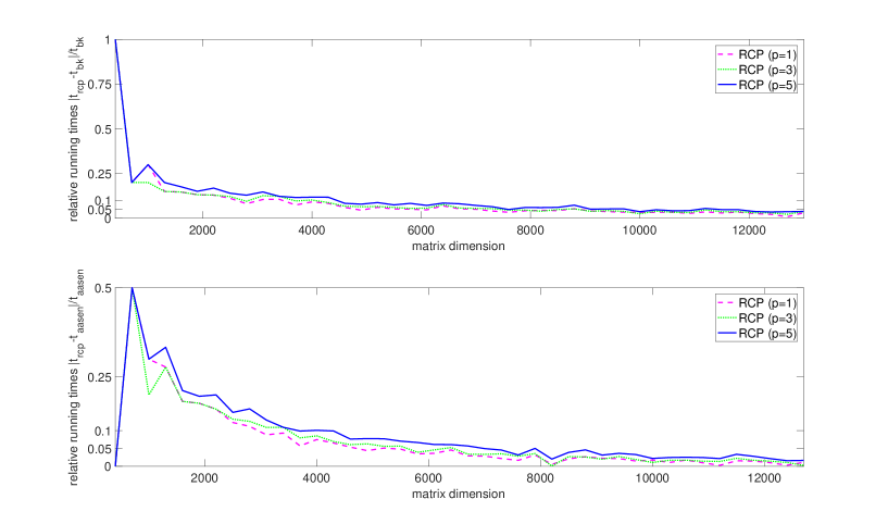
Refer to caption
Figure 7: Relative running times between RCP with three different value of p𝑝p and BK (Aasen) for Type 666 matrices.
Refer to caption
Figure 8: Results for Type 666 matrices with different p𝑝p. The top left plot shows the growth factor ρ𝜌\rho in the factorization of A𝐴A as defined by (25), the top right one shows the backward error in the solution of Ax=b𝐴𝑥𝑏Ax=b as defined by (24), the bottom left one shows the 111-norm of L𝐿L, and the bottom right one shows the 111-norm of inverse of L𝐿L.
Refer to caption
Figure 9: Results for Type 111 matrices. The top left plot shows the growth factor ρ𝜌\rho in the factorization of A𝐴A as defined by (25) and (26), the top right one shows the backward error in the solution of Ax=b𝐴𝑥𝑏Ax=b as defined by (24), the bottom left one shows the 111-norm of L𝐿L, and the bottom right one shows the 111-norm of inverse of L𝐿L.
Refer to caption
Figure 10: Running times for Type 222 matrices.
Refer to caption
Figure 11: Growth factor and backward error for matrices of Type 333 through 888. The left half plots show the element growth factor in the factorization of A𝐴A as defined by (25) and (26), and the right half ones show the backward error as defined by (24). Element growth factors of Type 444, Type 555 and Type 888 increase linearly, and the other three are small.
Refer to caption
Figure 12: L1subscriptnorm𝐿1\|L\|_{1} and L11subscriptnormsuperscript𝐿11\|L^{-1}\|_{1} for matrices of Type 333 through 888. The left half plots show the values of L1subscriptnorm𝐿1\|L\|_{1}, and the right half ones show the value of L11subscriptnormsuperscript𝐿11\|L^{-1}\|_{1}. All these results increase linearly.
Refer to caption
Figure 13: Results for Type 999 matrices. The top left plot shows the growth factor ρ𝜌\rho in the factorization of A𝐴A as defined by (25) and (26), the top right one shows the backward error in the solution of Ax=b𝐴𝑥𝑏Ax=b as defined by (24), the bottom left one shows the 111-norm of L𝐿L, and the bottom right one shows the 111-norm of inverse of L𝐿L.
Refer to caption
Figure 14: Results for Type 101010 matrices. The top left plot shows the growth factor ρ𝜌\rho in the factorization of A𝐴A as defined by (25) and (26), the top right one shows the backward error in the solution of Ax=b𝐴𝑥𝑏Ax=b as defined by (24), the bottom left one shows the 111-norm of L𝐿L, and the bottom right one shows the 111-norm of inverse of L𝐿L.

6 Conclusions

In this paper, we have introduced the randomized complete pivoting (RCP) algorithm for computing the LDLT𝐿𝐷superscript𝐿𝑇LDL^{T} factorization of a symmetric indefinite matrix. We developed a theoretical high-probability element growth factor upper bound for RCP, that is compatible to that of GECP. Moreover, we performed an error analysis to demonstrate the numerical stability of RCP. In our numerical experiments, RCP is as stable as Gaussian elimination with complete pivoting, yet only slightly slower than Bunch-Kaufman algorithm and Aasen’s algorithm.

References

  • [1] J. O. Aasen, On the reduction of a symmetric matrix to tridiagonal form, BIT Numerical Mathematics, 11 (1971), pp. 233–242.
  • [2] E. Anderson, Z. Bai, C. Bischof, L. S. Blackford, J. Demmel, J. Dongarra, J. Du Croz, A. Greenbaum, S. Hammarling, A. McKenney, et al., LAPACK Users’ guide, SIAM, 1999.
  • [3] M. Arioli, M. Baboulin, and S. Gratton, A partial condition number for linear least squares problems, SIAM Journal on Matrix Analysis and Applications, 29 (2007), pp. 413–433.
  • [4] R. I. Arriaga and S. Vempala, An algorithmic theory of learning: Robust concepts and random projection, in Foundations of Computer Science, 1999. 40th Annual Symposium on, IEEE, 1999, pp. 616–623.
  • [5] C. Ashcraft, R. G. Grimes, and J. G. Lewis, Accurate symmetric indefinite linear equation solvers, SIAM Journal on Matrix Analysis and Applications, 20 (1998), pp. 513–561.
  • [6] M. Baboulin, D. Becker, G. Bosilca, A. Danalis, and J. Dongarra, An efficient distributed randomized algorithm for solving large dense symmetric indefinite linear systems, Parallel Computing, 40 (2014), pp. 213–223.
  • [7] M. Baboulin, J. Dongarra, J. Herrmann, and S. Tomov, Accelerating linear system solutions using randomization techniques, ACM Transactions on Mathematical Software (TOMS), 39 (2013), p. 8.
  • [8] M. Baboulin, J. Dongarra, A. Rémy, S. Tomov, and I. Yamazaki, Dense symmetric indefinite factorization on gpu accelerated architectures, in International Conference on Parallel Processing and Applied Mathematics, Springer, 2015, pp. 86–95.
  • [9] M. Benzi, G. H. Golub, and J. Liesen, Numerical solution of saddle point problems, Acta numerica, 14 (2005), pp. 1–137.
  • [10] Å. Björck, Numerical methods for least squares problems, SIAM, 1996.
  • [11] V. I. Bogachev and V. I. Bogachev, Gaussian measures, vol. 62, American Mathematical Society Providence, 1998.
  • [12] J. R. Bunch, Analysis of the diagonal pivoting method, SIAM Journal on Numerical Analysis, 8 (1971), pp. 656–680.
  • [13] J. R. Bunch and L. Kaufman, Some stable methods for calculating inertia and solving symmetric linear systems, Mathematics of computation, (1977), pp. 163–179.
  • [14] J. R. Bunch and B. N. Parlett, Direct methods for solving symmetric indefinite systems of linear equations, SIAM Journal on Numerical Analysis, 8 (1971), pp. 639–655.
  • [15] T. A. Davis and Y. Hu, The university of florida sparse matrix collection, ACM Transactions on Mathematical Software (TOMS), 38 (2011), p. 1.
  • [16] I. T. Dimov, Monte Carlo methods for applied scientists, World Scientific, 2008.
  • [17] J. J. Dongarra, C. B. Moler, J. R. Bunch, and G. W. Stewart, LINPACK users’ guide, SIAM, 1979.
  • [18] Z. Drmač and Z. Bujanović, On the failure of rank-revealing qr factorization software–a case study, ACM Transactions on Mathematical Software (TOMS), 35 (2008), p. 12.
  • [19] A. Druinsky and S. Toledo, The growth-factor bound for the bunch-kaufman factorization is tight, SIAM Journal on Matrix Analysis and Applications, 32 (2011), pp. 928–937.
  • [20] I. S. Duff and J. K. Reid, The multifrontal solution of indefinite sparse symmetric linear, ACM Transactions on Mathematical Software (TOMS), 9 (1983), pp. 302–325.
  • [21] G. H. Golub and C. F. Van Loan, Matrix computations, vol. 3, JHU Press, 2012.
  • [22] M. Gu, Subspace iteration randomization and singular value problems, SIAM Journal on Scientific Computing, 37 (2015), pp. A1139–A1173.
  • [23] N. Halko, P.-G. Martinsson, and J. A. Tropp, Finding structure with randomness: Probabilistic algorithms for constructing approximate matrix decompositions, SIAM review, 53 (2011), pp. 217–288.
  • [24] N. J. Higham, Stability of the diagonal pivoting method with partial pivoting, SIAM Journal on Matrix Analysis and Applications, 18 (1997), pp. 52–65.
  • [25] N. J. Higham, Accuracy and stability of numerical algorithms, SIAM, 2002.
  • [26] N. J. Higham, The matrix computation toolbox for MATLAB (version 1.0), Manchester Centre for Computational Mathematics, 2002.
  • [27] R. A. Horn and C. R. Johnson, Matrix analysis, Cambridge university press, 2012.
  • [28] W. B. Johnson and J. Lindenstrauss, Extensions of lipschitz mappings into a hilbert space, Contemporary mathematics, 26 (1984), p. 1.
  • [29] C. Kenney, A. J. Laub, and M. Reese, Statistical condition estimation for linear least squares, SIAM Journal on Matrix Analysis and Applications, 19 (1998), pp. 906–923.
  • [30] J. W. Liu, A partial pivoting strategy for sparse symmetric matrix decomposition, ACM Transactions on Mathematical Software (TOMS), 13 (1987), pp. 173–182.
  • [31] M. W. Mahoney et al., Randomized algorithms for matrices and data, Foundations and Trends® in Machine Learning, 3 (2011), pp. 123–224.
  • [32] P.-G. Martinsson, V. Rokhlin, and M. Tygert, A randomized algorithm for the decomposition of matrices, Applied and Computational Harmonic Analysis, 30 (2011), pp. 47–68.
  • [33] C. Melgaard and M. Gu, Gaussian elimination with randomized complete pivoting, arXiv preprint arXiv:1511.08528, (2015).
  • [34] J.-C. Nédélec, Acoustic and electromagnetic equations: integral representations for harmonic problems, vol. 144, Springer Science & Business Media, 2001.
  • [35] J. Nocedal and S. Wright, Springer series in operations research and financial engineering, Numerical Optimization, (1999).
  • [36] D. S. Parker, Random butterfly transformations with applications in computational linear algebra, Tech. Report CSD-950023, Computer Science Department, UCLA, 1995.
  • [37] S. S. Vempala, The random projection method, vol. 65, American Mathematical Soc., 2005.
  • [38] J. H. Wilkinson, Error analysis of direct methods of matrix inversion, Journal of the ACM (JACM), 8 (1961), pp. 281–330.
  • [39] F. Woolfe, E. Liberty, V. Rokhlin, and M. Tygert, A fast randomized algorithm for the approximation of matrices, Applied and Computational Harmonic Analysis, 25 (2008), pp. 335–366.
  • [40] J. Xiao and M. Gu, Spectrum-revealing cholesky factorization for kernel methods, in Data Mining (ICDM), 2016 IEEE 16th International Conference on, IEEE, 2016, pp. 1293–1298.
  • [41] D. Zwillinger and S. Kokoska, CRC standard probability and statistics tables and formulae, Crc Press, 1999.