Structured Slow Solar Wind Variability:
Streamer-Blob Flux Ropes and Torsional Alfvén Waves

Abstract

The slow solar wind exhibits strong variability on timescales from minutes to days, likely related to magnetic reconnection processes in the extended solar corona. Higginson et al. (2017b) presented a numerical magnetohydrodynamic simulation which showed interchange magnetic reconnection is ubiquitous and most likely responsible for releasing much of the slow solar wind, in particular along topological features known as the Separatrix-Web (S-Web). Here, we continue our analysis, focusing on two specific aspects of structured slow solar wind variability. The first type is present in the slow solar wind found near the heliospheric current sheet, and the second we predict should be present everywhere S-Web slow solar wind is observed. For the first type, we examine the evolution of three-dimensional magnetic flux ropes formed at the top of the helmet streamer belt by reconnection in the heliospheric current sheet (HCS). For the second, we examine the simulated remote and in situ signatures of the large-scale torsional Alfvén wave (TAW) which propagates along an S-Web arc to high latitudes. We describe the similarities and differences between the reconnection-generated flux ropes in the HCS, which resemble the well-known ”streamer blob” observations, and the similarly structured TAW. We discuss the implications of our results for the complexity of the HCS and surrounding plasma sheet, and the potential for particle acceleration, as well as the interchange reconnection scenarios which may generate TAWs in the solar corona. We discuss predictions from our simulation results for the dynamic slow solar wind in the extended corona and inner heliosphere.

1 Introduction

The global magnetic structure of the solar corona directly determines the structure of the solar wind outflow (e.g. Zirker, 1977; Axford et al., 1999; Antiochos et al., 2007, 2011; Cranmer, 2012). Decades of in situ observations have shown that the heliospheric structure and solar wind properties reflect the coronal magnetic structure of its origin (Zurbuchen, 2007). The high-speed solar wind that originates from coronal holes is relatively fast, cool, and homogeneous (Geiss et al., 1995; McComas et al., 2002), and the low-speed solar wind originating from or near large-scale closed flux systems (i.e. coronal streamers) is hotter, denser, and exhibits considerably more variability in its in situ plasma, field, and composition measurements (Gosling, 1997; Zurbuchen et al., 2000, 2002; Kepko et al., 2016). While a stationary, steady-state slow speed wind can be obtained in open flux regions at the boundaries of helmet streamers due to the large expansion factors (Arge & Pizzo, 2000; Cranmer, 2012; Wang et al., 2012), research increasingly suggests that it is composition which categorizes the solar wind, rather than speed (e.g. Stakhiv et al., 2015, 2016). Therefore, reproducing the variability in the slow solar wind plasma composition during the formation of solar wind has become essential. Dynamic magnetic reconnection scenarios for the release of coronal plasma from the closed magnetic field into the solar wind must be invoked (e.g. Wang et al., 2000; Antiochos et al., 2011; Higginson et al., 2017a; Uritsky et al., 2017).

Evidence for the importance of magnetic reconnection during the formation of the solar wind exists in both remote and in situ observations. High quality, high cadence white-light coronagraph data and recent heliospheric imaging data have shown that the slow solar wind originating near the coronal helmet streamer belt includes an intermittent and highly structured outflow of intensity enhancements across spatial scales, the largest of which are known as “streamer blobs,” which move outwards into the heliosphere with the bulk outflow of the solar wind (Sheeley et al., 1997, 1999; Sheeley & Wang, 2007; Sheeley et al., 2009; Song et al., 2009; Rouillard et al., 2010a, b; Viall & Vourlidas, 2015; Sanchez-Diaz et al., 2017). At the same time, in situ measurements farther out in the heliosphere also find small-scale magnetic flux ropes in the slow solar wind. Cartwright & Moldwin (2010a) described the initial Moldwin et al. (2000) observations as “[having] bipolar field rotations coincident with a core field enhancement and were on the order of tens of minutes duration and displayed the signature of a force-free, symmetric magnetic flux rope.” There has been considerable progress in the characterization of plasma and field properties of these events, including large statistical surveys (Feng et al., 2007, 2008; Cartwright & Moldwin, 2008, 2010a; Kilpua et al., 2009; Foullon et al., 2011; Janvier et al., 2014a, b; Feng & Wang, 2015; Feng et al., 2015; Yu et al., 2014, 2016). Many of these researchers (e.g. Janvier et al., 2014b; Yu et al., 2014, and others) have discussed the similarities and differences between small-scale flux ropes and the larger interplanetary coronal mass ejections (ICMEs) which contain a coherent in situ flux rope structure, called magnetic clouds (Burlaga et al., 1981; Marubashi, 1986; Burlaga, 1988; Lepping et al., 1990). Considerable progress has also been made toward linking these small flux rope in situ signatures, which are almost always observed in the slow solar wind associated with the heliospheric plasma sheet, to their source region in the solar corona. For example, Kilpua et al. (2009) trace a number of their small-scale flux rope events back to their origin at the potential field source surface (PFSS) sector boundaries (i.e. the helmet streamer belt), and the detailed analyses of Rouillard et al. (2011) directly image the coronal and heliospheric propagation of several in situ small-scale flux rope transients via running-difference tracks of their corresponding coronal streamer blobs in the STEREO Heliospheric Imager data.

The studies above all focus on magnetic flux ropes as the main source of magnetic field variability, but there is a second type of variability which can be linked back to solar wind formation. A number of researchers have examined periods of in situ solar wind data that have some or all of the signatures of small-scale flux rope events but are actually consistent with large-scale torsional Alfvén waves (TAWs) instead (e.g. Gosling et al., 2010; Marubashi et al., 2010; Cartwright & Moldwin, 2010a; Yu et al., 2014). The schematic of the coherent magnetic field rotation of a propagating torsional Alfvén wave presented by Marubashi et al. (2010) illustrates just how similar to a twisted flux rope these signatures may be. The main difference between the two is the direction of the core field. While the core field of a traditional flux rope is transverse to the direction of propagation (at least at formation), that of a torsional Alfvén wave is along the radial solar wind magnetic field, allowing the twist component of the flux rope-like structure to propagate along the core magnetic field as a wave. One key discriminator between this type of propagating “pseudo-flux rope” wave and a true flux rope is the Alfvénicity of the period in question. Yu et al. (2014), and others, have argued if the structured, rotation-like $\delta\boldsymbol{B}$ fluctuations are highly correlated with $\delta\boldsymbol{V}$ during the event interval, then the period of interest should probably be considered a propagating Alfvénic disturbance rather than a small-scale flux rope. As we will discuss herein, it is extremely likely that both these torsional Alfvén waves and the traditional small-scale flux rope transients are generated by coronal magnetic reconnection processes.

In this paper we extend the analysis of our numerical magnetohydrodynamic (MHD) simulation of reconnection and evolution at the Separatrix-web (S-web; Antiochos et al., 2011) described by Higginson et al. (2017b), hereafter referred to as Paper I, by focusing on the two aspects of structured slow solar wind variability described above, flux ropes within the heliospheric current sheet (HCS) and torsional Alfvén waves, both of which are present in our simulation. The paper is organized as follows. In section 2, we briefly recap the Paper I MHD simulation set up and our previous results. In section 3, we present synthetic remote and in situ signatures of our simulated HCS flux ropes and discuss the relevant properties of the streamer blob and small-scale flux rope observations. We also examine the large-scale TAW which results from our boundary driving and propagates along the S-Web arc to high latitudes, and discuss its similarities to in situ measurements. For both of these types of structured variability, we present visualizations of magnetic field line connectivity and evolution from a set of stationary observers in the heliosphere, akin to orbiting spacecraft. In section 4, we discuss our results and their implications for the upcoming Parker Solar Probe and Solar Orbiter missions, and in section 5, we present our conclusions.

2 Numerical Methods

The numerical simulation presented in Paper I is run using the Adaptively Refined MHD Solver (ARMS; DeVore & Antiochos, 2008). ARMS solves the equations of ideal MHD in 3D spherical coordinates using a finite-volume, flux-corrected transport scheme (DeVore, 1991). Our initial magnetic field configuration, given in Antiochos et al. (2011), consists of an elongated coronal-hole corridor extending southwards from a polar coronal hole, like the one shown in Figures 1A and 1B. The black magnetic field lines in Figure 1C show the outline of the simulated coronal hole from Paper I on the solar surface.

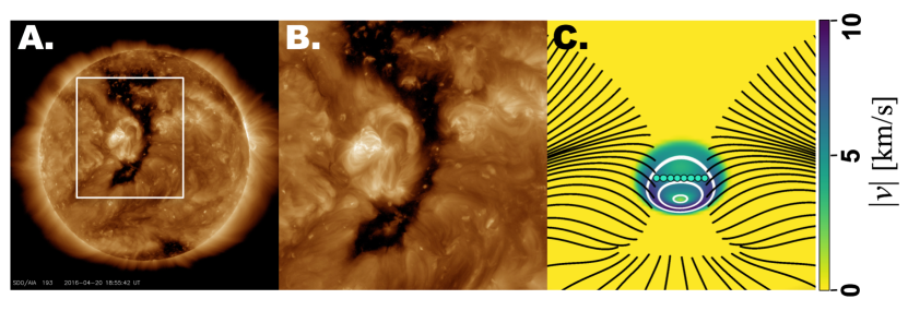
Figure 1: A. Solar Dynamics Observatory EUV image of the Sun. The coronal hole appears dark relative to the surrounding corona. B. Zoom-in of white box from A. C. Simulated S-Web corridor. Black magnetic field lines outline the boundary of the polar and low-latitude open regions and the connecting open-field corridor on the surface. Cyan dots cross the corridor. Yellow/green/purple shading indicates the driving velocity magnitude applied in the simulations; white velocity streamlines on the surface show the rotational motion. (Reproduced from Paper I.)

The computational domain is defined as $r\in[1R_{\odot},30R_{\odot}]$, $\theta\in[11.25^{\circ},168.75^{\circ}]$, where $\theta$ is measured from the north pole, and $\phi\in[-90^{\circ},90^{\circ}]$. We use logarithmic grid spacing in the radial direction and linear spacing in $\theta$ and $\phi$. The grid is constructed using the PARAMESH package (MacNeice et al., 2000) from $8\times 7\times 8$ root blocks with 5 additional levels of static grid refinement specified over the coronal-hole corridor and resulting S-Web arc. The effective grid resolution is thus $1024\times 896\times 1024$ in the highest refinement regions. While there is no explicit physical resistivity included in ideal MHD, we note that necessary and stabilizing diffusion terms are inherent in the numerical scheme allowing for an effective numerical resistivity when the magnetic field gradients are compressed to the scale of the grid. The $(r,\theta,\phi)$ boundary conditions and our implementation of the Parker (1958) isothermal solar wind background are described by Masson et al. (2013), Karpen et al. (2017), and Higginson et al. (2017a). The solar wind is initialized with a $T=1$ MK isothermal atmosphere and the density at the lower radial boundary is set to $\rho_{\odot}/m_{p}=3.6\times 10^{9}$ cm^-3.

Paper I described the evolution and dynamics of interchange reconnection that takes place along a high-latitude S-Web arc formed by a narrow coronal-hole corridor after it was perturbed by a supergranular-like, flux-preserving rotational flow. The colored contours in Figure 1C show the magnitude of the rotational flow imposed across the coronal-hole corridor and the white streamlines show the direction of the flow. This flow lies in the $\theta$,$\phi$ plane only and is constructed so as to preserve the normal component of the magnetic field during the evolution. In order to satisfy

$$\frac{\partial B_{r}}{\partial t}=-\nabla_{\perp}\cdot\left(\mathbf{v_{\perp}}B_{r}\right)=0,$$ (1)

we choose $\bf{v_{\perp}}$ to be equal to the curl of a radial vector,

$$\bf{v_{\perp}}=\nabla_{\perp}\times\left(\psi,0,0\right).$$ (2)

We define $\psi$ as a function of $\theta$, $\phi$, and $t$,

$$\psi\left(\theta,\phi,t\right)\equiv V_{0}f(t)g(\xi)h(\beta),$$ (3)

where

$$f(t) = \frac{1}{2}\left[1-\cos\left(2\pi k\frac{t-t_{0}}{t_{2}-t_{1}}\right)\right],$$ (4)

$$g(\xi) = \frac{(m+l+1)}{(l+1)}\left[1-\xi^{2(l+1)}\right]-\left[1-\xi^{2(m+l+1)}\right],$$ (5)

$$h(\beta) = \frac{1}{2}\beta^{2}.$$ (6)

In the equations above, the parameters $k$, $t_{0}$, $t_{1}$, $t_{2}$ are set to ramp up the flow to maximum velocity from zero and then from that velocity back to zero. This ensures that all disturbances are smooth. The equation for $g(\xi)$ defines an annulus in spatial coordinate $\xi$, where

$$\xi^{2}\equiv 4\left(\frac{\theta-\theta_{0}}{\theta_{2}-\theta_{1}}\right)^{2}+4\left(\frac{\phi-\phi_{0}}{\phi_{2}-\phi_{1}}\right)^{2}.$$ (7)

The location of the flow annulus is determined by the limits $\theta_{1}$, $\theta_{2}$, and $\phi_{1}$, $\phi_{2}$, with coordinate $\left(\theta_{0},\phi_{0}\right)$ representing the center. The thickness and radial velocity profile of the flow annulus are defined by $m$ and $l$. We set $m=l=1$ to yield a thick annulus with a velocity peak at the center of the annulus. In the equation for $h(\beta)$, $\beta$ is the magnetic field coordinate between minimum and maximum strengths, i.e.,

$$\beta\equiv\max\left(\min\left(B_{r},B_{2}\right),B_{1}\right).$$ (8)

where we chose $B_{1}$ and $B_{2}$ so that $\beta=B_{r}$ everywhere in our flow region.

This flow ($v_{max}<9kms^{-1}$) was applied to the lower boundary and rotated the field in a 100 Mm region by 180 degrees, effectively moving flux from one side of the corridor to the other. The cyan dots drawn across Figure 1C represent the foot points of the blue magnetic field lines shown in Figure 2. The boundary motion of the magnetic field introduces a significant twist component which then propagates into the heliosphere along these open field lines as a large-scale TAW.

3 MHD Simulation Results

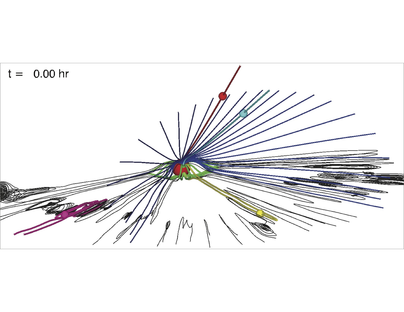
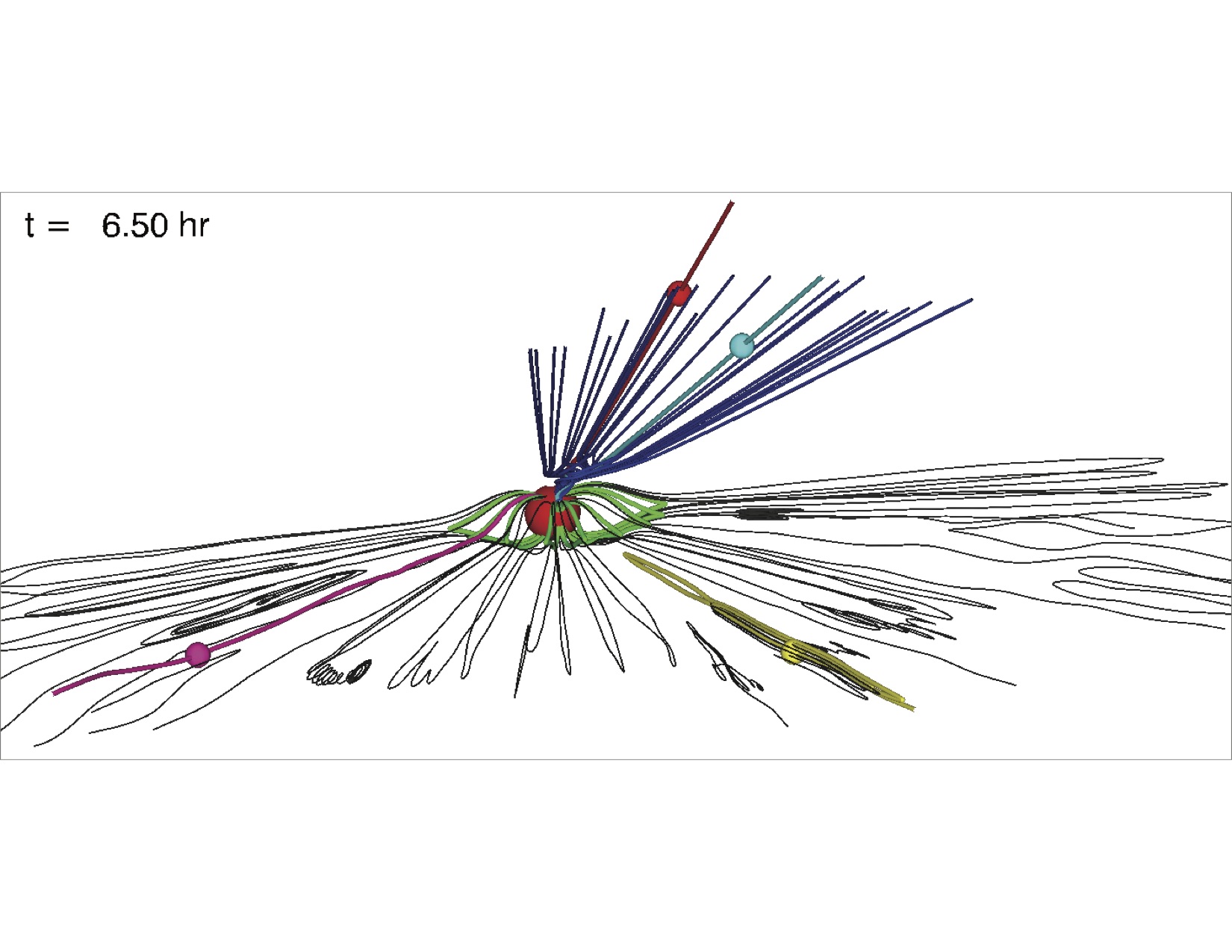
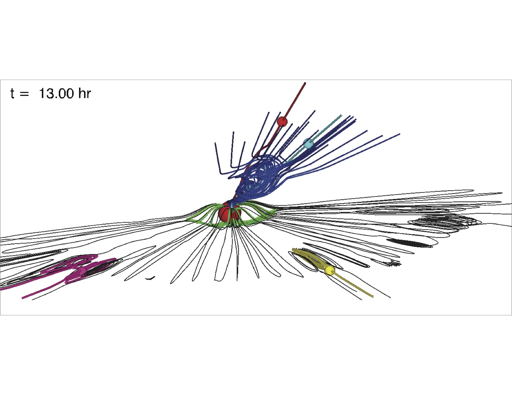
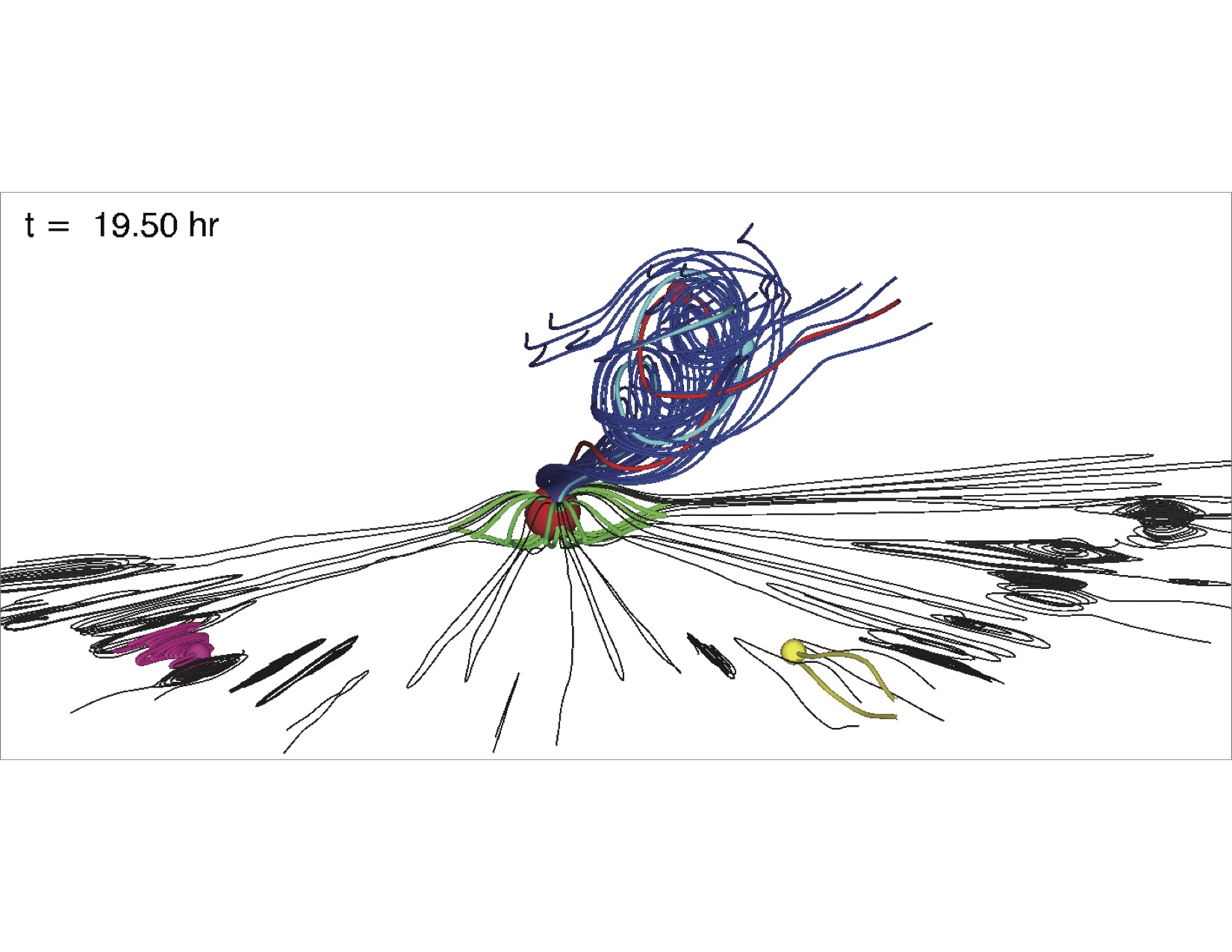
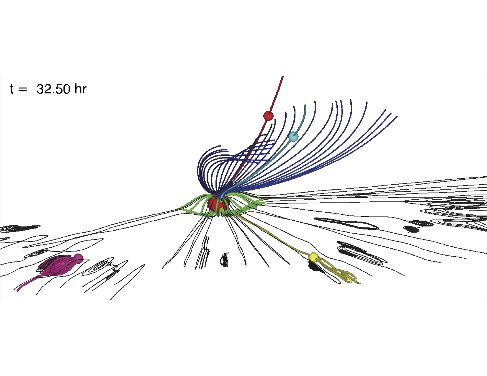
Figure 2: Six panels showing the evolution of streamer blobs in the HCS and the TAW. The black magnetic field lines show the interconnected blobs emanating from the top of the helmet streamer (shown in green). The blue field lines drawn from the surface show the S-Web arc and the TAW generated by the rotational photospheric driver. Four stationary observers and their magnetic field line connectivities are plotted in magenta, yellow, red, and light blue.
(An animation of this figure is available.)

3.1 System Evolution and the Magnetic Connectivity of Stationary Observers

The six frames of Figure 2 show the overall domain and system evolution throughout our simulation (also discussed in Paper I). The green magnetic field lines outline the location of the helmet streamer, whose outer limit marks the start of the heliospheric plasma sheet. The black magnetic field lines, drawn from within the equatorial plane beyond 20 $R_{\odot}$, show the stream of blobs emanating from the streamer top at all longitudes continuously emitted throughout the simulation. This the first type of structured slow solar wind variability which is discussed in Section 3.2. When the the top of the helmet streamer is stretched outwards by the solar wind, it eventually becomes thin enough to reconnect, allowing the top of the helmet streamer to pinch off and form a small flux rope, which then moves outwards with the solar wind. The scale of these blobs in our simulation is set by the scale of the magnetic reconnection, which occurs at the scale of the grid. While the size of these blobs will vary with Lundquist number in our simulation, we will show that they have similar signatures to the streamer blobs observed by Sheeley et al. (2009), Rouillard et al. (2011), and others.

Also shown in Figure 2, rooted in the northern hemisphere at the lower boundary, are blue magnetic field lines drawn across the coronal-hole corridor. These field lines map out the high-latitude S-Web arc before the driving takes place ($t=0.00~{}hr$) and their foot points do not move throughout the simulation. Paper I showed why this S-Web arc is predicted to also correspond to locations of slow solar wind, along with the HCS. When the rotational motion takes place at the lower boundary between times $t=0.00~{}hr$ and $t=9.5~{}hr$, it launches an Alfvén wave onto the open magnetic field lines. The start of this wave is visible at time $t=6.50~{}hr$ and the subsequent snapshots in Figure 2 show its propagation through the domain. By time $t=32.50~{}hr$ most of this Alfvén wave structure has left the domain through the outer boundary at 30 $R_{\odot}$. Note that while this wave slightly distorts the HCS, the blobs shown within the heliospheric plasma sheet in Figure 2 remain largely unaffected by the wave. We will argue that the properties of our simulation’s large-scale TAW are qualitatively similar to the in situ observations of “pseudo-flux rope” waves and that these structures can result, on a smaller scale than shown here, from interchange reconnection predicted to take place in regions which correspond to an S-Web arc (e.g. Paper I, and references therein),. This is the second type of structured slow solar wind variability which is discussed in Section 3.3.

Finally, Figure 2 also shows the location and magnetic field line connectivity of four stationary observers marked by colored spheres. The instantaneous magnetic field line from each of these points is plotted in the same color scheme. The red (S1) and light blue (S2) observers along the S-Web arc are located at $\boldsymbol{r}_{S1}=(21R_{\odot},54^{\circ},0^{\circ})$ and $\boldsymbol{r}_{S2}=(21R_{\odot},60^{\circ},6^{\circ})$ respectively. S1 and S2 show the connectivity of a point in space as the TAW passes over it, in contrast to the dark blue field lines which show the magnetic field connectivity drawn from the surface. The magenta (E1) and yellow (E2) observers lie in the ecliptic plane, located at $\boldsymbol{r}_{E1}=(21R_{\odot},90^{\circ},-53^{\circ})$ and $\boldsymbol{r}_{E2}=(21R_{\odot},90^{\circ},7^{\circ})$ respectively. They sample the 3D flux ropes that form in the HCS which correspond to the well-known streamer blobs. We encourage the reader to see the animation of Figure 2 that is included as an online electronic supplement to the article.

3.2 Variability in the HCS-Associated Wind: Generation and Propagation of Small-Scale Flux Ropes

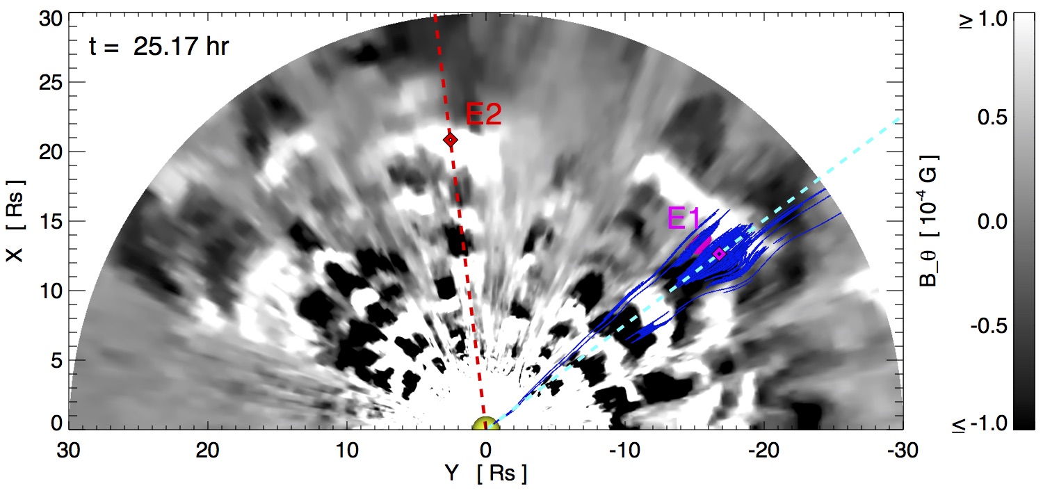
Figure 3: An equatorial cut of $B_{\theta}$ viewed from above. The greyscale is heavily saturated such that it shows the sign of $B_{\theta}$. Each pair of black and white signals show the location of a blob in the HCS. Also shown are observers E1 and E2 and their radial vectors. Observer E1 is accompanied by blue magnetic field lines drawn for context.
(An animation of this figure is available.)

Figure 2 illustrates the dynamic and 3D nature of the blobs originating from the top of the helmet streamer. Figure 3, an equatorial cut of $B_{\theta}$ where the viewer is looking down on the HCS from the north pole, shows how these blobs fill the heliospheric plasma sheet. By showing $B_{\theta}$ in saturated greyscale, we highlight the locations where $B_{\theta}$ is either into or out of the page (i.e. northward or southward toward either pole). The leading edge of the structures have a $B_{\theta}$ component in one direction, while the trailing edges have the opposite, as expected from small flux ropes. In Figure 3, the leading edges have a positive $B_{\theta}$ (towards the north pole) and are shown in white. The blobs show no longitudinal preferences and move outwards in a continuous radial stream. Also shown in Figure 3 are the locations of two of the stationary observers E1 (magenta) and E2 (now shown in red) from Figure 2. The dotted lines shown in light blue and red represent the rays drawn from the Sun through the observers which were used to generate the simulated remote observations below. Blue magnetic field lines are also shown around E1 for context.

Clearly visible in Figure 3 is the longitudinal extent of the blobs. While the flux rope structures observed by Sheeley et al. (2009) can be tens of degrees wide, here we see smaller longitudinal widths of less than ten degrees. This is due to the negligible longitudinal guide field present in our symmetric helmet streamer. As the streamer top stretches out and eventually pinches off, forming a small flux rope, the shear component at the top of the helmet streamer becomes the core field of the flux rope, oriented perpendicular to the radial direction. In our simulation this component is generally small. Small longitudinal widths are consistent, however, with the multi-spacecraft in situ observations of small flux ropes in the solar wind by Kilpua et al. (2009). They observed that spacecraft separated by only a few degrees would often not encounter the same transient structure, and even if they did, the features could be quite different, suggesting a small width and high level of complexity within the flux ropes.

Figure 4: Left panel: in situ data detected by observer E1 corresponding to a single, well-structured streamer blob flux rope event (denoted by the vertical dashed lines). Right panel: the zoomed-in, 3D view of E1 from Figure 3 showing a portion of the magenta magnetic field line traced from E1 and the surrounding blue field lines showing the HCS flux rope structure.
(An animation of this figure is available)

In Figure 4 we take a closer look at the structure of a single streamer-blob flux rope. The right panel shows a frame from the animation of Figure 3, but now the viewer is looking edge on to the equatorial plane and watching the flux rope as it moves towards the outer boundary in the bottom right corner. The black and white transparent surface is the same $B_{\theta}$ from Figure 3 as are the magenta and blue magnetic field lines surrounding the observer E1. Here we also see, especially in the animation of this figure, that these flux ropes are not isolated, disconnected structures, but rather that the magnetic connectivity often threads multiple flux ropes. This is due to the three dimensionality of the pinching-off reconnection of the helmet streamer, in particular, different longitudes pinch-off reconnect at different times, meaning they retain some partial magnetic connection to nearby regions. Because each event is fully 3D and different than its neighbors, the overall effect is that of interconnectedness, rather than fully independent and separate flux rope structures. This could also be due to, or exacerbated by, dynamic magnetic reconnection which takes place between solar wind structures as the blob moves outwards in the solar wind, as discussed by Gosling et al. (2006) in observations and Higginson et al. (2017a) in simulations.

In the left panel of Figure 4 we plot the in situ parameters observed by E1 as the flux rope sweeps across it. From top to bottom we plot number density ($n_{p}$), plasma beta ($\beta=8\pi P/B^{2}$), and the three components of the magnetic field ($B_{r}$, $B_{\theta}$, $B_{\phi}$), where $B_{r}$ is towards or away from the Sun, $B_{\theta}$ is towards the north or south pole, and $B_{\phi}$ completes the right-handed coordinate system. The red line indicates the time shown in the right panel, and the blue dashed lines bound the event. Our flux rope blobs move outwards with the solar wind and show a smooth and organized rotation in the magnetic field. Here, $B_{\theta}$ starts out positive before flipping smoothly through zero at the core of the structure to become negative on the other side. Our density shows a slight increase, on the order of 6%, at the center of the flux rope. The magnitude of this density fluctuation is almost certainly underestimated with our isothermal solar wind model. Additionally, the behavior of the plasma $\beta$ in our simulation flux rope is opposite that reported in the literature, due to our lack of a flux rope core (axial) field. Our magnetic field effectively goes to zero at the center of the structure, causing the spike in plasma $\beta$. However, the bipolar magnetic field rotation signature in our streamer-blob flux ropes closely resembles those reported by Cartwright & Moldwin (2008).

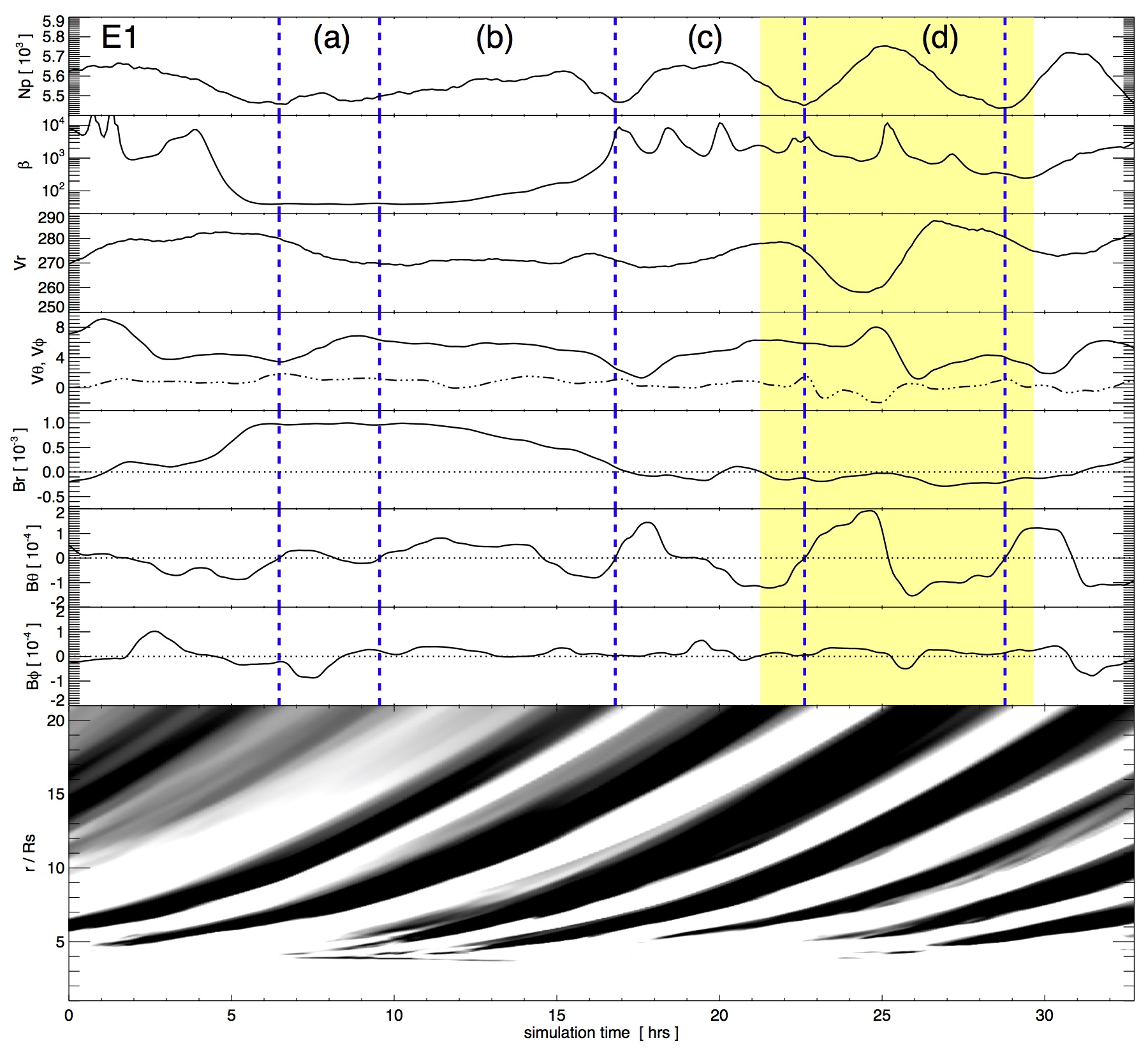
Figure 5: The full time series of $N_{p}$, $\beta$, $\boldsymbol{V}$, $\boldsymbol{B}$ at E1. The bottom panel shows the height-time J-map (after Sheeley et al., 1999) of the Figure 3 ${B_{\theta}}$ quantity that define the 3D flux rope boundaries (also shown as dashed vertical blue lines).

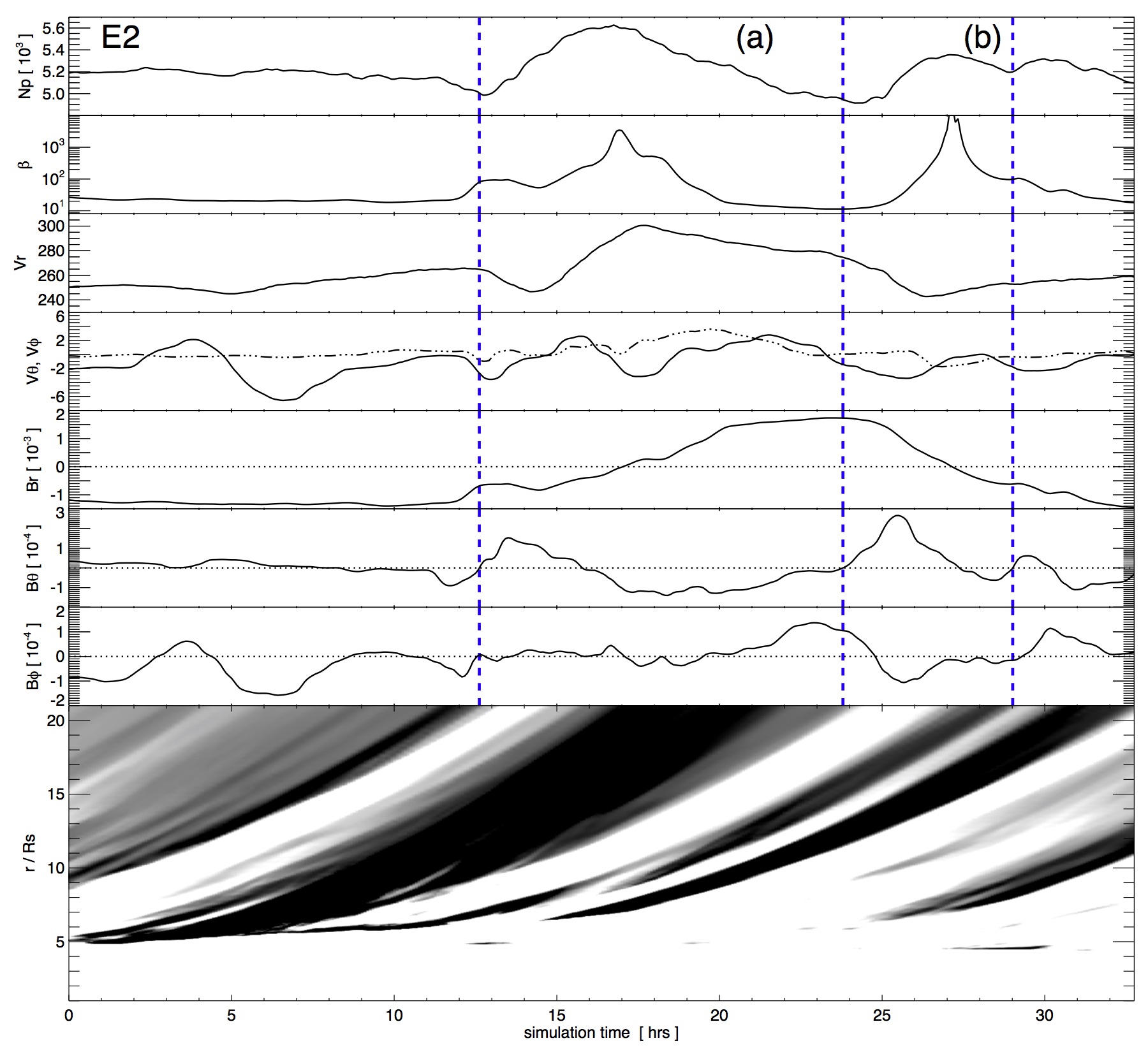
Figure 6: The E2 plasma and magnetic field time series and J-map, in the same format as Figure 5.

Figure 5 shows the in-situ parameters number density ($N_{p}$), plasma beta ($\beta$), radial velocity ($V_{r}$), latitudinal and longitudinal velocity ($V_{\theta}$ and $V_{\phi}$), and the three components of the magnetic field ($B_{r}$, $B_{\theta}$, $B_{\phi}$) detected at E1 for $\sim$33 hours of the simulation. The bottom panel shows a height-time J-map (after Sheeley et al., 1999) of $B_{\theta}$ along the dotted light blue line from Figure 3 at the position angle of E1, where the vertical axis is height above the solar surface and simulation time is along the horizontal axis. The time period shown in Figure 4 is highlighted in yellow in Figure 5. The top of the J-map is set at the radial height of E1 (21 $R_{\odot}$) so that the top of the J-map aligns with the in situ data plotted above it. The blue dotted lines from Figure 4 which bound the event are also plotted in Figure 5. Additional blue lines are plotted to show the boundary between flux ropes, defined as the transition from negative to positive $B_{\theta}$. Figure 5 cleanly illustrates the steady and continuous nature of the blobs, their smooth motion outwards with the solar wind velocity (seen in the J-map), and also shows how magnetically complex the structures can be (in situ data) while retaining their smooth rotations in magnetic field.

Figure 6 shows the same quantities as shown in Figure 5 for the observer E2. The radial cut used for the J-map in the bottom panel is indicated by the red dotted line in Figure 3. Comparing Figures 3, 5, and 6 it is clear that the blobs occur at all longitudes and have similar properties. The radial extent of some of the blobs in Figure 6 varies more than the blobs in Figure 5 because in this location the HCS becomes slightly distorted, developing a slight “ballerina skirt ruffle,” and is shifted to slightly lower latitudes. Rather than cutting straight through the center of the blobs, the E2 observer essentially skims across the top of the HCS structures instead. This also seen in the $B_{r}$ time series—$B_{r}$ is a constant, negative polarity, until the first flux rope boundary at $t\sim 12.5$ $hr$ and afterwards, $B_{r}$ shows two consecutive HCS crossings and three easily-identified streamer-blob flux ropes. The movement of the HCS is due to the driving and resulting dynamics in the simulation, which will be discussed in Section 3.3 below.

3.3 Variability in the S-Web-Associated Wind: Generation and Propagation of a Large-Scale Torsional Alfvén Wave

As described in Paper I, to simulate the effect of supergranular driving on an S-Web coronal-hole corridor we placed a $1\pi$ rotation in $(\theta,\phi)$ on the solar surface, which overlapped with the closed magnetic field on both sides of the coronal-hole corridor. This motion displaced the coronal hole boundary and generated a plethora of interchange reconnection as the boundary relaxed to its new equilibrium state. This interchange reconnection is responsible for the release of coronal plasma from the closed field regions onto open field lines all along the S-Web arc (Paper I) and is the origin of the slow solar wind found far the heliospheric current sheet. The effect of this photospheric rotation on the open magnetic field was to launch a large-scale Alfvén wave which propagated outwards into the heliosphere.

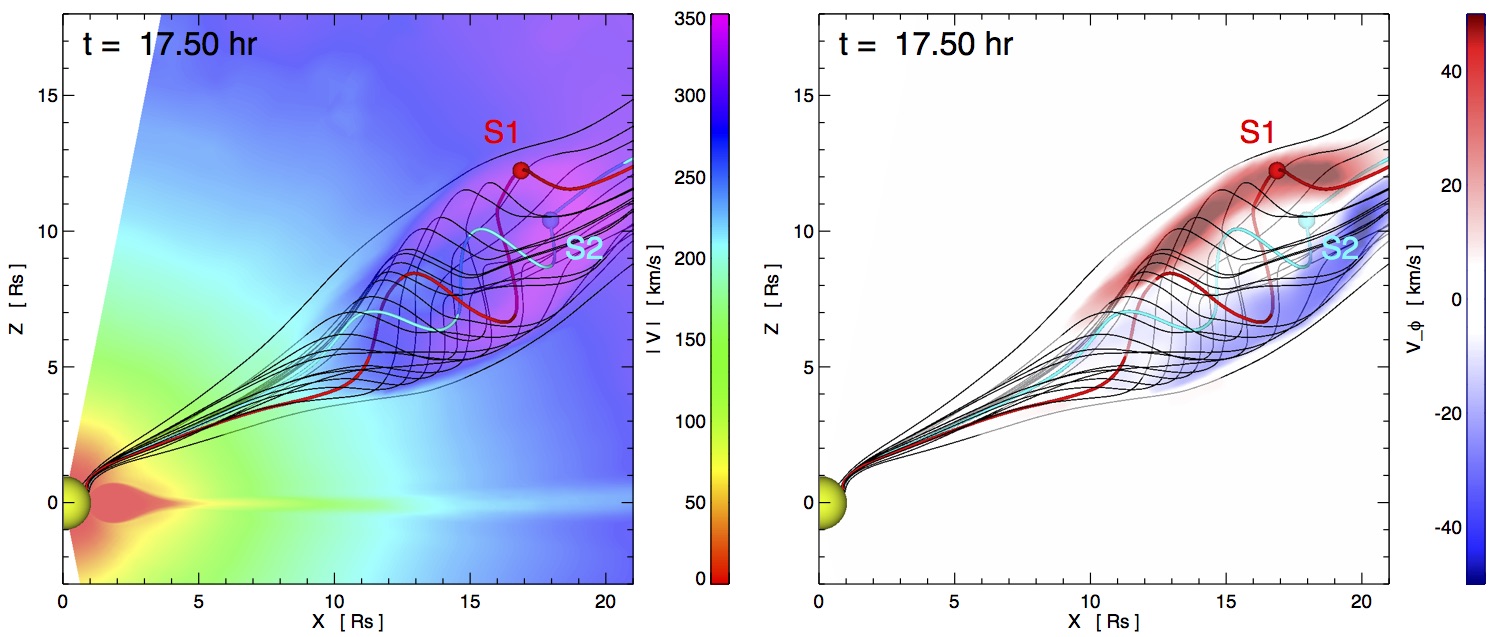
Figure 7: Longitudinal cut at $\phi=0$ of $|V|$ (left) and $V_{\phi}$ (right) showing the TAW propagating through the S1 (red), S2 (light blue) observation points. Representative surrounding magnetic field lines are also shown in black to illustrate the “pseudo-flux rope” structure of the TAW.
(An animation of this figure is available)

Figure 7 shows this TAW after the surface rotation has stopped and the wave has propagated out to $\sim$15 $R_{\odot}$. The left panel shows contours of velocity magnitude ($|V|$) in a slice through zero longitude. The right panel shows contours of $V_{\phi}$ (into and out of the page) at the same locations. The black magnetic field lines are shown for context around the two observers S1 and S2, originally shown in Figure 2. The animation included online shows the generation and propagation of this wave for the whole simulation period. Here in this 3D view, the resemblance of this structure to a flux rope is on display; the magnetic field lines seem to coil around an axial magnetic field in the direction of propagation.

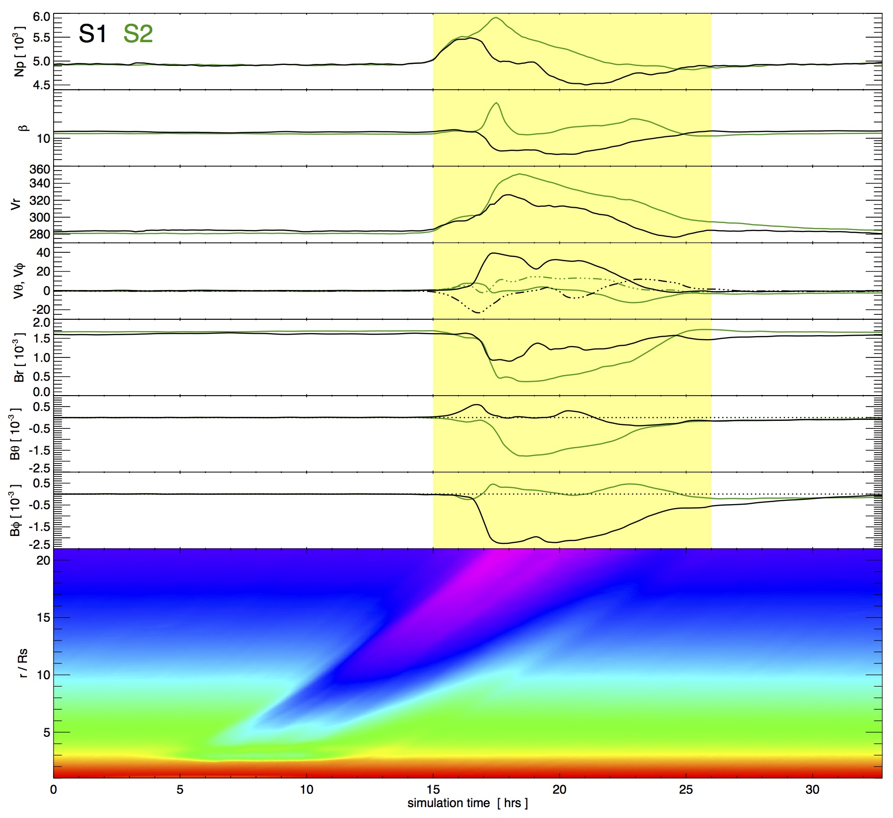
Figure 8: The full time series of $N_{p}$, $\beta$, $\boldsymbol{V}$, $\boldsymbol{B}$ at S1 (black) and S2 (green) observation points. The height-time J-map plot through S1 of ${|V|}$ shows the radial propagation and evolution of the large-scale TAW.

To compare this structure to the flux ropes seen in the HCS, we again plot the in situ data from the observers in Figure 8. Here we show the time series for the full $\sim$33 simulated hours of $N_{p}$, $\beta$, $\boldsymbol{V}$, $\boldsymbol{B}$ at S1 (black) and S2 (green) in panels 1-7. The bottom panel shows the J-map of $|V|$ using a ray through S1 and the color scale from Figure 7. As before, the top of the J-map lines up with the location of the observer for comparison to the in situ time series. The time period during which the TAW is passing over S1 is highlighted in yellow. Immediately obvious is the scale of the transient above the background solar wind. The density and all three of the velocity components show much larger enhancements than the flux rope structures. This is due in part to the unrealistically large driving motion which we used at the surface due to numerical constraints, however, we will argue below that this structures of this type should be visible at smaller scales in the solar wind. Examining the magnetic field components we see that while the flux rope structures exhibited a smooth rotation through zero, this structure shows a rotation offset from zero in $B_{\phi}$ for S1 and $B_{\theta}$ for S2. The S1 and S2 observation points are at the center and edge of the wave structure in longitude respectively but are roughly equivalent distances from the central radial axis of the large-scale propagating TAW disturbance. Hence, the S1, S2 profiles of $B_{\phi}$ and $B_{\theta}$ represent an $\sim$90^∘ phase-shift in the fluctuation quantities. While multipoint in situ measurements would certainly help to differentiate between TAWs and small-scale flux ropes, the magnetic field rotation offset from zero signature by itself is generally not sufficient. This is even more relevant since we know in our simulation that the observers are traversing the TAW structure axially instead of cutting across its diameter as in the case of our flux ropes in the HCS.

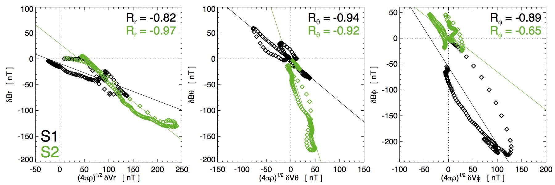
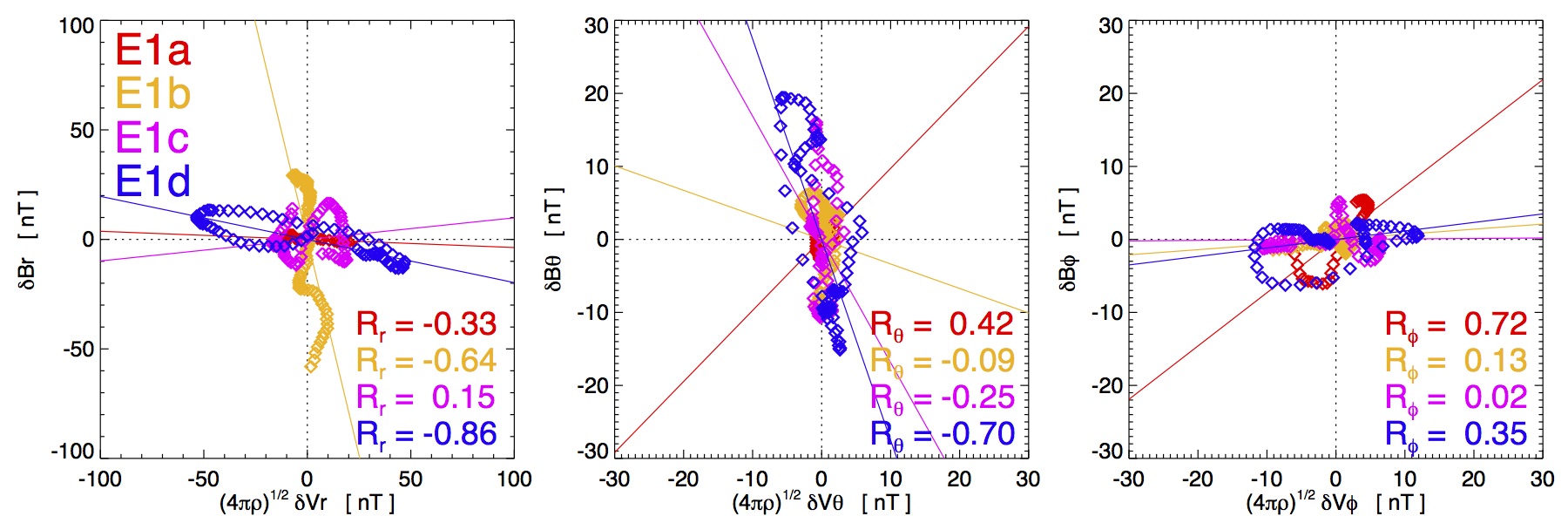
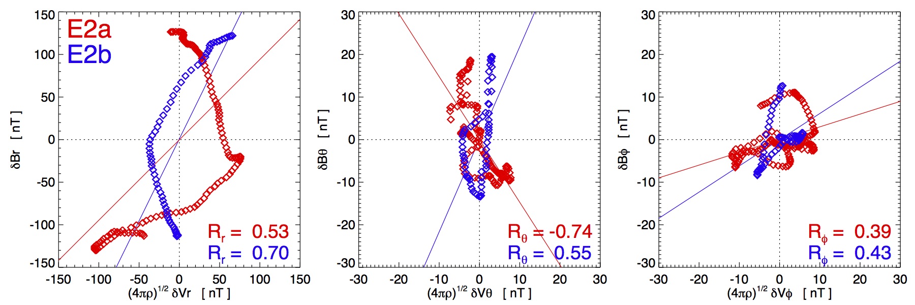
Figure 9: Left, middle, and right panels show the Alfvénicity plot of $\delta\boldsymbol{B}$ vs. $(4\pi\rho)^{1/2}\;\delta\boldsymbol{V}$ in their $r$, $\theta$, and $\phi$ components, respectively for each of the events. The linear fits are plotted with solid colored lines and the correlation coefficients are listed. The TAW event observed by S1 (black) and S2 (green) are shown in the top row. The four flux-rope blobs observed by observer E1 are shown in red, yellow, pink, and blue in the middle row. The two flux-rope blobs observed by E2 are shown in the bottom row in red and blue. The high correlation coefficients of TAW event in the top row show that it is highly Alfvénic.

To differentiate between a flux rope and a TAW we must examine the Alfvénicity of the structure during the time period highlighted in yellow in Figure 8. The TAW identification criteria for in situ data used by Yu et al. (2014, 2016) is the magnitude of the correlation between the magnetic field fluctuations $\delta\boldsymbol{B}$ and the density-normalized velocity fluctuations $(4\pi\rho)^{1/2}\;\delta\boldsymbol{V}$. The fluctuations are calculated in the usual fashion as $\delta\boldsymbol{B}\equiv\boldsymbol{B}-\langle\boldsymbol{B}\rangle$ and $\delta\boldsymbol{V}\equiv\boldsymbol{V}-\langle\boldsymbol{V}\rangle$ where the mean value is the average (or a sufficiently long running-average) of the time series. The period of interest is considered Alfvénic if all three of the fluctuation vector components have correlation magnitudes of $|R|>0.5$ or if two components are strongly correlated with $|R|>0.6$ and the third component is at least weakly correlated with $|R|>0.3$.

Figure 9 plots $\delta\boldsymbol{B}$ against $(4\pi\rho)^{1/2}\;\delta\boldsymbol{V}$ for each TAW and flux rope event. The fluctuation vectors are separated into their respective $r$-components (left panel), $\theta$-components (middle panel) and $\phi$-components (right panel). The TAW observed by S1 (black) and S2 (green) is analyzed in the top row. The middle row shows the analysis of the four flux rope events observed by E1 (as delineated in Figure 5) in red, yellow, pink, and blue, and the bottom row shows the two flux rope events observed by E2 (as delineated in Figure 6) in red and blue. The correlation coefficients for each component in each interval are listed in each plot. The linear fits to the component pairs are also shown in each panel as dashed lines. For observer S1 (S2) which measured the TAW, we obtained correlation magnitude values that far exceed the observational Alfvénic threshold criteria, as expected: $|R_{r}|$ = 0.82 (0.97), $|R_{\theta}|$ = 0.94 (0.92), and $|R_{\phi}|$ = 0.89 (0.65). Each of the HCS flux rope event intervals (E1a$-$d, E2a,b) fail to pass the empirical in-situ criteria for being considered Alfvénic.

We also computed the Walén number $R_{W}(t)$ (Walén, 1944) throughout each event interval, defined as

$$\big{\langle}R_{W}\big{\rangle}\equiv\bigg{\langle}\frac{(4\pi\rho)^{1/2}\delta V_{\perp}}{\delta B_{\perp}}\bigg{\rangle},$$ (9)

where $\delta V_{\perp}=(\delta V_{\theta}^{2}+\delta V_{\phi}^{2})^{1/2}$, $\delta B_{\perp}=(\delta B_{\theta}^{2}+\delta B_{\phi}^{2})^{1/2}$, and the $\langle\cdot\rangle$ brackets denote the event-average of the synthetic in-situ time series. An ideal Alfvén wave in an isotropic plasma would have $R_{W}=1$. The minimum, maximum, mean, and standard deviation of $R_{W}$ measured by each observer over the course of each event are listed in Table 1. Here we see that each HCS flux-rope interval (event type “blob”) has a much higher, non-Alfvénic maximum $R_{W}$ value than either of the TAW event intervals (type “wave”), and that the wave events show $R_{W}(t)$ distributions closer to $\lesssim 1$ than the blob events.

The analysis of the Walén numbe and the component correlation coefficients (Figure 9) analyze only the fluctuation magnitudes, so we also look at the the relative phase difference between the $\delta\boldsymbol{B_{\perp}}$ and $\delta\boldsymbol{V_{\perp}}$ components to provide additional information about the Alfvénicity of our intervals. For a radial propagating disturbance, the fluctuation phase angles are defined as

$$\alpha_{B}=\sin^{-1}\left[{\frac{\delta B_{\theta}}{\delta B_{\perp}}}\right]\;,\;\;\;\alpha_{V}=\sin^{-1}\left[{\frac{\delta V_{\theta}}{\delta V_{\perp}}}\right]\;,$$ (10)

which yield a relative phase difference of

$$\Delta\Omega=\left\{\begin{array}[]{lcl}\left|\alpha_{B}-\alpha_{V}\right|&\mathrm{for}&\left|\alpha_{B}-\alpha_{V}\right|\leq\pi\\ 2\pi-\left|\alpha_{B}-\alpha_{V}\right|&\mathrm{for}&\left|\alpha_{B}-\alpha_{V}\right|>\pi\end{array}\right.,$$ (11)

with $\Delta\Omega\in[0,\pi]$ for $\alpha_{B}$, $\alpha_{V}$ $\in[0,2\pi]$. Here an ideal Alfvén wave will have a phase difference between the field and velocity components of $\Delta\Omega=\pi=180^{\circ}$. These quantities are also listed in Table 1 and plotted in Figure 10, along with the pictorial hodograms.

Figure 10 shows the hodogram and relative phase angle evolution for each of the observed structures. The TAW observations by S1 and S2 are in the top row, the blob observations from E1a-d are in the second and third rows, and the blob observations from E2a,b are in the bottom row. The red-to-yellow (blue-to-green) transition in the hodograms on the left shows the time evolution in the velocity (magnetic) fluctuations, and the phase angle between these at each time is plotted in black on the right. The phase angle for the TAW observations shows highly Alfvénic behavior, with the phase angle oscillating close to $\Delta\Omega=\pi=180^{\circ}$ for most of the time period before dropping off, while the behavior for the blob observations shows no such pattern, indicating a non-Alfvénic structure.

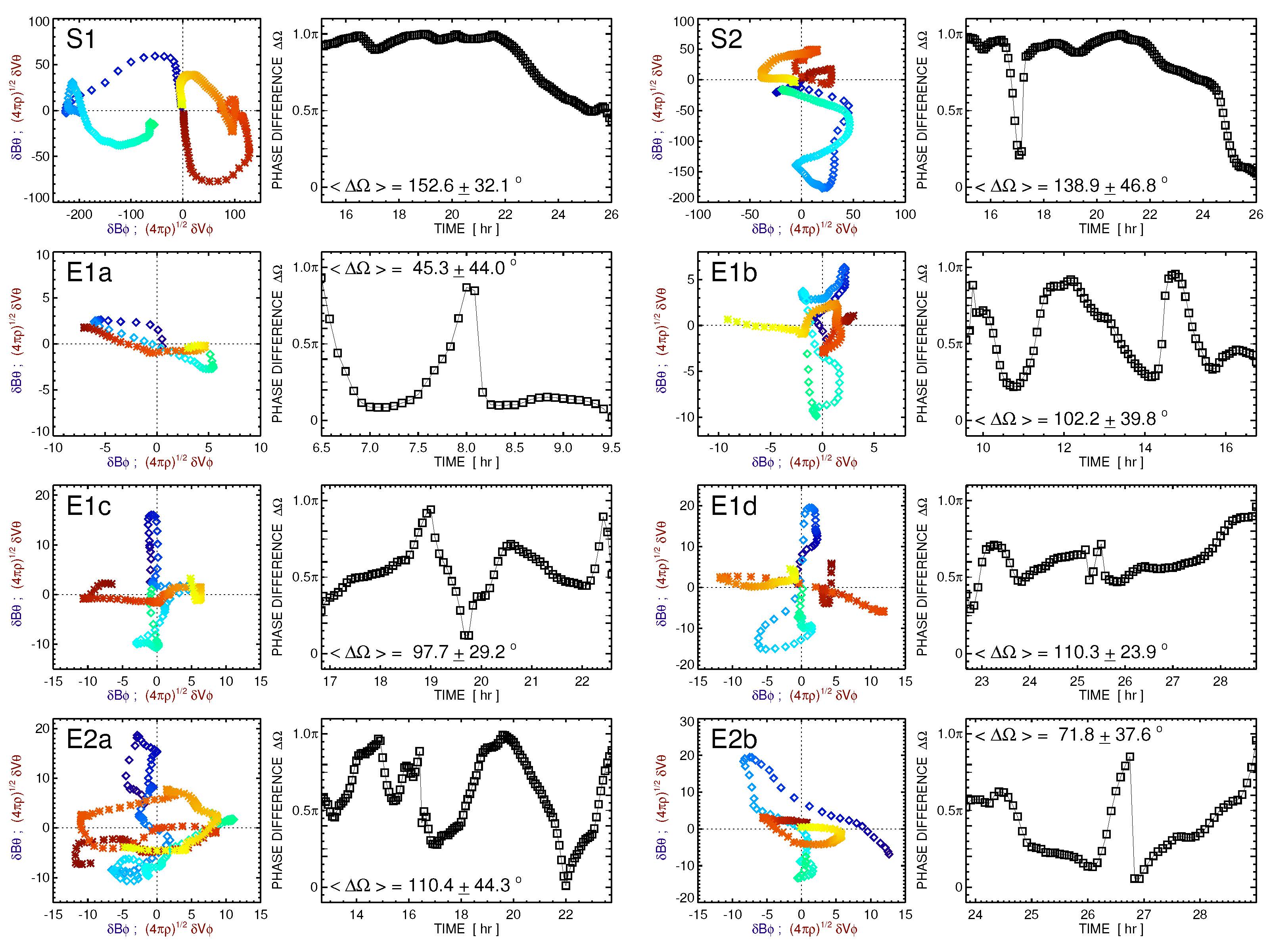
Figure 10: Hodograms and phase angle evolution of the perpendicular components of the magnetic field $\delta\boldsymbol{B_{\perp}}$ and normalized velocity fluctuations $(4\pi\rho)^{1/2}\delta\boldsymbol{V_{\perp}}$ in our TAW samples S1, S2 (top row), and each of the equatorial streamer blob events, E1a-d (second and third rows) and E2a,b (forth row). The colors in each hodogram show the temporal evolution of the magnetic fluctuations (blue-to-green) and the velocity fluctuations red-to-yellow over the duration of the events. The relative phase difference $\Delta\Omega$ between the $\delta\boldsymbol{B_{\perp}}$ and $\delta\boldsymbol{V_{\perp}}$ components are plotted next to each hodogram (also summarized in Table 1)

.

Label	$\min{R_{W}}$	$\max{R_{W}}$	$\langle R_{W}\rangle\pm\sigma_{R_{W}}$	$\langle\Delta\Omega\rangle\pm\sigma_{\Delta\Omega}$	Type
S1	0.09	1.51	0.56 $\pm$ 0.39	$152\pm 32\;\;^{\circ}$	wave
S2	0.11	1.93	0.52 $\pm$ 0.33	$139\pm 47\;\;^{\circ}$	wave
E1a	1.71	25.3	6.9 $\pm$ 5.8	$45\pm 44\;^{\circ}$	blob
E1b	1.82	18.7	4.3 $\pm$ 2.9	$102\pm 40\;^{\circ}$	blob
E1c	0.33	26.6	3.8 $\pm$ 4.6	$98\pm 29\;^{\circ}$	blob
E1d	0.30	21.9	2.3 $\pm$ 3.3	$110\pm 23\;^{\circ}$	blob
E2a	0.04	16.1	1.3 $\pm$ 2.1	$110\pm 44\;^{\circ}$	blob
E2b	0.30	3.6	0.94 $\pm$ 0.71	$72\pm 38\;^{\circ}$	blob

Table 1: Event-averaged Walén Numer ($R_{W}$) and relative phase difference ($\Delta\Omega$) between $\delta\boldsymbol{B_{\perp}}$ and $\delta\boldsymbol{V_{\perp}}$

for the TAW and streamer blob events. More Alfvénic features have a Walén number closer to 1 and a relative phase difference closer to 180^∘.

4 Origins of Structured Variability in the Slow Solar Wind

4.1 Streamer Blobs as 3D Magnetic Flux Ropes from Reconnection in the HCS

As seen in Sections 3.1 and 3.2, our simulation has streamer blobs throughout the HCS which are all formed through helmet streamer pinch-off reconnection (Sheeley et al., 1997; Wang et al., 2000). Earlier 2D and 2.5D MHD simulations have also observed this process (e.g. Einaudi et al., 1999, 2001; Endeve et al., 2003, 2004; Rappazzo et al., 2005; Lapenta & Restante, 2008; Allred & MacNeice, 2015). Our results suggest that the HCS may be a region of consistently complex topology, with threaded flux ropes creating a dynamic layer of slow solar wind surrounding the HCS.

Such a scenario has been presented by Crooker et al. (1996, 2004) who argue that the in situ observations of the HCS and plasma sheet represent a tangled network of squashed flux ropes. Our 3D magnetic islands are lacking the observed axial field enhancement, $B_{\phi}$, corresponding to a guide field component during the reconnection at the streamer belt cusp. However, our current simulation results are certainly consistent with the Crooker et al. (1996) scenario, especially if we were to take into account the heliospheric evolution of a more realistic HCS shape, fast coronal hole wind, and the resulting stream structure and interaction regions. Recent results indicate that turbulence can generate a whole distribution of small-flux ropes in the solar wind throughout the heliosphere (e.g Zheng & Hu, 2018), but our simulation results show that 3D streamer blob pinch-off reconnection at the Sun can contribute a significant component of this variability.

While the tangled nature of the flux ropes should be consistent with the real Sun and heliosphere, the idea that these flux ropes should all be completely squashed is not. The helicity condensation picture of Antiochos (2013) predicts that there ought to be a guide field component from the shear which should be continuously generated by convective photospheric evolution. This shear is transported through the closed flux region towards the closed-open flux boundary of the helmet streamer belt (see also Knizhnik et al., 2015, 2017). A distribution of various guide field component strengths along the closed-open flux boundary will become a distribution of axial/core field strengths during the magnetic island flux rope formation. Therefore, we expect a less-idealized simulation to generate streamer blob magnetic structures in the slow wind around the HCS that both match the observed, well-defined in situ small-scale flux ropes with an enhanced core field as well as flux ropes without core fields that may be more easily compressed into planar-like structures during their heliospheric evolution. Our simulation results, combined with the in situ observations of un-squashed flux ropes (as argued by Moldwin et al., 2000), suggest that both may be present in the HSC-associated slow solar wind, essentially all of the time.

One of the major implications of a highly structured heliospheric plasma sheet filled with magnetic islands is related to energetic particle acceleration in the heliosphere. The formation and evolution of magnetic island structures have been suggested as processes for accelerating particles in and around magnetic reconnection sites (e.g. Drake et al., 2006; Dahlin et al., 2014; Guidoni et al., 2016; Khabarova et al., 2016, and references therein) where particles can be accelerated via the curvature drift and Fermi-reflection associated with the contraction of the island flux surfaces.

Our particular situation in which we have many dynamic islands with potentially small guide fields is an interesting one to consider. Dahlin et al. (2014, 2015, 2016) used particle-in-cell simulations to show that when the guide field is much larger than the reconnecting field then electron acceleration via the Fermi mechanism is suppressed. On the other hand, turbulent 3D simulations show that with no guide field at all electron acceleration doesn’t occur either. Too little guide field and particle acceleration is negligible; too much guide field and not only is the particle lost from the island structure quickly, but there is less flux surface contraction, limiting the contribution of the second mechanism.

A complex network of streamer-blob flux ropes in the heliospheric plasma sheet with a range of guide fields is an ideal breeding ground for particle acceleration. Indeed, Khabarova et al. (2015, 2016) have performed calculations of the energization due to magnetic islands to explain the in situ observations of keV–MeV particles in the HCS and discussed the importance of this suprathermal component to generating the observed intensities of CIR and CME shock-associated SEPs.

4.2 Torsional Alfvén Waves as “Pseudo-Flux Rope” Structures from Interchange Reconnection

The TAW in our simulation, described in Section 3.3, was generated by a large-scale rotational motion on the solar surface. Because this rotational motion was much larger and more coherent than any photospheric motion on the real Sun, it produced an isolated, large-scale TAW signature which was easily investigated. While there are many observations of TAWs in the solar wind (Yu et al. 2016; also the STEREO PLASTIC Level 3 data product) there is some inherent uncertainty associated with both visual inspection and automated identification and classification of small-scale flux ropes and TAWs (e.g. Feng et al., 2010; Cartwright & Moldwin, 2010b; Yu et al., 2014). There is even a documented case of a TAW within a small-scale flux rope (Gosling et al., 2010). Here, we were able to analyze an oversized but clean sample TAW and compare it with HCS-associated structures under the same conditions.

One proposed mechanism for TAW creation at the Sun includes the reconnection associated with solar jets (Shibata & Uchida, 1986). Explosive jet observations provide some of the most direct measurements of the Alfvénic propagation of magnetic field line twist into the solar corona and into the heliosphere (see Raouafi et al., 2016; Uritsky et al., 2017, and references therein). The high-resolution simulations by Wyper et al. (2016) resolved both the large-scale twist jet eruption along the external spine line and small-scale, 3D flux rope islands with localized, concentrated twist which were formed in the reconnection current sheet layer during the breakout/interchange reconnection prior to the main eruption (see also Lynch et al., 2014; Wyper et al., 2017). Wyper et al. (2016) described the propagation of the magnetic island’s localized twist along the newly reconnected field lines as TAWs. Similar interchange reconnection dynamics are also expected over a distribution of larger spatial scales from active region flux systems (Török et al., 2009; Archontis & Hood, 2013; Moreno-Insertis & Galsgaard, 2013; Lynch et al., 2014) to coronal pseudostreamers (Török et al., 2011; Zuccarello et al., 2012; Masson et al., 2014; Edmondson & Lynch, 2017; Wang & Hess, 2018).

While most of these simulations showing TAW formation are driven by either emerging twisted flux or twisting up existing flux distributions (i.e. introducing some form of twist that is ultimately transferred via reconnection onto open field lines), there is increasing evidence that sufficiently resolved reconnection processes—even in planar geometries—will introduce a twist component during the formation and ejection of 3D magnetic island plasmoids. For example, the simulations of Edmondson & Lynch (2017) investigated the generation of 3D magnetic island flux ropes from externally-driven interchange reconnection in a coronal pseudostreamer geometry. These small-scale flux rope structures had a significant localized twist component even though the simulation boundary flows were purely translational (i.e. no twist component). As the islands were ejected within the reconnection exhaust into the open field region, their core/axis tended to realign towards the open field direction so that the localized twist component was able to more freely propagate away as “pseudo-flux rope” TAWs. Edmondson & Lynch (2017) argued this evolution represents the small-scale, reconnection-generated 3D magnetic island manifestation of the larger-scale Shibata & Uchida (1986) twist-jet scenario.

Since a wide variety of reconnection scenarios can generate these “pseudo flux rope” and flux rope signatures and the observed variability and composition of the slow solar wind strongly suggests its origin is related to magnetic reconnection (Zurbuchen, 2007; Zhao et al., 2017), we conjecture that these periods of structured and coherent variability in the slow solar wind should also exhibit temporal coincidence with other plasma and composition signatures of reconnection. Encouragingly, there are observational studies show that this may be the case (Feng & Wang, 2015; Feng et al., 2015; Yu et al., 2016; Kepko et al., 2016; Wang & Hess, 2018). These TAWs, generated by interchange reconnection in the solar corona, should therefore be observed in the S-Web-associated slow solar wind discussed by Antiochos et al. (2011), Higginson et al. (2017a) and Paper I, both along S-Web arcs and in the HCS.

5 Conclusions

We have reported on two distinct features of structured slow solar wind variability present in the Paper I MHD simulation. First, we presented the analysis of the basic plasma and field structure of 3D, streamer-blob flux ropes created in the HCS by pinch-off reconnection at the helmet streamer cusp, which represents a critical missing component of solar wind modeling thus far. This form of solar wind variability must be included in future models in order to correctly simulate true heliospheric observations. Steady-state MHD models by their very nature can not include helmet streamer dynamics, which are observed both remotely and in-situ. Our dynamic simulation results are consistent with many aspects of the in situ observations of the small-scale magnetic flux ropes and suggest that even the simplest, equatorial heliospheric plasma sheet could be filled with tangled and intermingled flux rope structures, as in the Crooker et al. (1996) picture, making it a promising region for particle acceleration. Additionally, we discussed the lack of guide field in our helmet streamer and the flattened flux ropes we observed in the HCS. We predict that the guide field component of observed HCS flux ropes will be a direct measure of the helicity condensation rate at the open magnetic field boundary.

Second, we analyzed an idealized, large-scale TAW that propagates along the S-Web arc in the slow solar wind to high latitudes. We examined the similarities and differences of these Alfvénic field and plasma fluctuations to those in the HCS streamer-blob flux ropes and discussed interchange reconnection scenarios that are likely to result in generation of TAWs in the corona. These TAWs should be found in the slow solar wind all along the S-Web, both in S-Web arcs and the HCS, where interchange reconnection should be prevalent (Paper I). This type of variability observed in the slow solar wind is most likely formed in principio, and may hold important clues as to the different sources of different types of wind. Our simulation results and analysis are an important contribution towards characterizing the field and in situ plasma signatures predicted by the Antiochos et al. (2011) dynamic S-Web model in anticipation for the Parker Solar Probe and Solar Orbiter missions.

References

- Allred & MacNeice (2015) Allred, J. C., & MacNeice, P. J. 2015, Computational Science and Discovery, 8, 015002
- Antiochos (2013) Antiochos, S. K. 2013, ApJ, 772, 72
- Antiochos et al. (2007) Antiochos, S. K., DeVore, C. R., Karpen, J. T., & Mikić, Z. 2007, ApJ, 671, 936
- Antiochos et al. (2011) Antiochos, S. K., Mikić, Z., Titov, V. S., Lionello, R., & Linker, J. A. 2011, ApJ, 731, 112
- Archontis & Hood (2013) Archontis, V., & Hood, A. W. 2013, ApJ, 769, L21
- Arge & Pizzo (2000) Arge, C. N., & Pizzo, V. J. 2000, J. Geophys. Res., 105, 10465
- Axford et al. (1999) Axford, W. I., McKenzie, J. F., Sukhorukova, G. V., et al. 1999, Space Sci. Rev., 87, 25
- Burlaga et al. (1981) Burlaga, L., Sittler, E., Mariani, F., & Schwenn, R. 1981, J. Geophys. Res., 86, 6673
- Burlaga (1988) Burlaga, L. F. 1988, J. Geophys. Res., 93, 7217
- Cartwright & Moldwin (2008) Cartwright, M. L., & Moldwin, M. B. 2008, J. Geophys. Res., 113, 9105
- Cartwright & Moldwin (2010a) —. 2010a, J. Geophys. Res., 115, 8102
- Cartwright & Moldwin (2010b) —. 2010b, J. Geophys. Res., 115, A10110
- Cranmer (2012) Cranmer, S. R. 2012, Space Sci. Rev., 172, 145
- Crooker et al. (1996) Crooker, N. U., Burton, M. E., Phillips, J. L., Smith, E. J., & Balogh, A. 1996, J. Geophys. Res., 101, 2467
- Crooker et al. (2004) Crooker, N. U., Huang, C.-L., Lamassa, S. M., et al. 2004, J. Geophys. Res., 109, A03107
- Dahlin et al. (2014) Dahlin, J. T., Drake, J. F., & Swisdak, M. 2014, Physics of Plasmas, 21, 092304
- Dahlin et al. (2015) —. 2015, Physics of Plasmas, 22, 100704
- Dahlin et al. (2016) —. 2016, Physics of Plasmas, 23, 120704
- DeVore (1991) DeVore, C. R. 1991, Journal of Computational Physics, 92, 142
- DeVore & Antiochos (2008) DeVore, C. R., & Antiochos, S. K. 2008, ApJ, 680, 740
- Drake et al. (2006) Drake, J. F., Swisdak, M., Che, H., & Shay, M. A. 2006, Nature, 443, 553
- Edmondson & Lynch (2017) Edmondson, J. K., & Lynch, B. J. 2017, ApJ, submitted
- Einaudi et al. (1999) Einaudi, G., Boncinelli, P., Dahlburg, R. B., & Karpen, J. T. 1999, J. Geophys. Res., 104, 521
- Einaudi et al. (2001) Einaudi, G., Chibbaro, S., Dahlburg, R. B., & Velli, M. 2001, ApJ, 547, 1167
- Endeve et al. (2004) Endeve, E., Holzer, T. E., & Leer, E. 2004, ApJ, 603, 307
- Endeve et al. (2003) Endeve, E., Leer, E., & Holzer, T. E. 2003, ApJ, 589, 1040
- Feng & Wang (2015) Feng, H. Q., & Wang, J. M. 2015, ApJ, 809, 112
- Feng et al. (2007) Feng, H. Q., Wu, D. J., & Chao, J. K. 2007, J. Geophys. Res., 112, A02102
- Feng et al. (2010) —. 2010, J. Geophys. Res., 115, A10109
- Feng et al. (2008) Feng, H. Q., Wu, D. J., Lin, C. C., et al. 2008, J. Geophys. Res., 113, 12105
- Feng et al. (2015) Feng, H. Q., Zhao, G. Q., & Wang, J. M. 2015, J. Geophys. Res., 120, 10
- Foullon et al. (2011) Foullon, C., Lavraud, B., Luhmann, J. G., et al. 2011, ApJ, 737, 16
- Geiss et al. (1995) Geiss, J., Gloeckler, G., von Steiger, R., et al. 1995, Science, 268, 1033
- Gosling (1997) Gosling, J. T. 1997, in American Institute of Physics Conference Series, Vol. 385, Robotic Exploration Close to the Sun: Scientific Basis, ed. S. R. Habbal, 17–24
- Gosling et al. (2006) Gosling, J. T., McComas, D. J., Skoug, R. M., & Smith, C. W. 2006, Geophys. Res. Lett., 33, 17102
- Gosling et al. (2010) Gosling, J. T., Teh, W.-L., & Eriksson, S. 2010, ApJ, 719, L36
- Guidoni et al. (2016) Guidoni, S. E., DeVore, C. R., Karpen, J. T., & Lynch, B. J. 2016, ApJ, 820, 60
- Higginson et al. (2017a) Higginson, A. K., Antiochos, S. K., DeVore, C. R., Wyper, P. F., & Zurbuchen, T. H. 2017a, ApJ, 837, 113
- Higginson et al. (2017b) —. 2017b, ApJ, 840, L10
- Janvier et al. (2014a) Janvier, M., Démoulin, P., & Dasso, S. 2014a, Sol. Phys., 289, 2633
- Janvier et al. (2014b) —. 2014b, J. Geophys. Res., 119, 7088
- Karpen et al. (2017) Karpen, J. T., DeVore, C. R., Antiochos, S. K., & Pariat, E. 2017, ApJ, 834, 62
- Kepko et al. (2016) Kepko, L., Viall, N. M., Antiochos, S. K., et al. 2016, Geophys. Res. Lett., 43, 4089
- Khabarova et al. (2015) Khabarova, O., Zank, G. P., Li, G., et al. 2015, ApJ, 808, 181
- Khabarova et al. (2016) Khabarova, O. V., Zank, G. P., Li, G., et al. 2016, ApJ, 827, 122
- Kilpua et al. (2009) Kilpua, E. K. J., Luhmann, J. G., Gosling, J., et al. 2009, Sol. Phys., 256, 327
- Knizhnik et al. (2015) Knizhnik, K. J., Antiochos, S. K., & DeVore, C. R. 2015, ApJ, 809, 137
- Knizhnik et al. (2017) —. 2017, ApJ, 835, 85
- Lapenta & Restante (2008) Lapenta, G., & Restante, A. L. 2008, Annales Geophysicae, 26, 3049
- Lepping et al. (1990) Lepping, R. P., Burlaga, L. F., & Jones, J. A. 1990, J. Geophys. Res., 95, 11957
- Lynch et al. (2014) Lynch, B. J., Edmondson, J. K., & Li, Y. 2014, Sol. Phys., 289, 3043
- MacNeice et al. (2000) MacNeice, P., Olson, K. M., Mobarry, C., de Fainchtein, R., & Packer, C. 2000, Computer Physics Communications, 126, 330
- Marubashi (1986) Marubashi, K. 1986, Advances in Space Research, 6, 335
- Marubashi et al. (2010) Marubashi, K., Cho, K.-S., & Park, Y.-D. 2010, Twelfth International Solar Wind Conference, 1216, 240
- Masson et al. (2013) Masson, S., Antiochos, S. K., & DeVore, C. R. 2013, ApJ, 771, 82
- Masson et al. (2014) Masson, S., McCauley, P., Golub, L., Reeves, K. K., & DeLuca, E. E. 2014, ApJ, 787, 145
- McComas et al. (2002) McComas, D. J., Elliott, H. A., & von Steiger, R. 2002, Geophys. Res. Lett., 29, 1314
- Moldwin et al. (2000) Moldwin, M. B., Ford, S., Lepping, R., Slavin, J., & Szabo, A. 2000, Geophys. Res. Lett., 27, 57
- Moreno-Insertis & Galsgaard (2013) Moreno-Insertis, F., & Galsgaard, K. 2013, ApJ, 771, 20
- Parker (1958) Parker, E. N. 1958, ApJ, 128, 664
- Raouafi et al. (2016) Raouafi, N. E., Patsourakos, S., Pariat, E., et al. 2016, Space Science Reviews, 201, 1
- Rappazzo et al. (2005) Rappazzo, A. F., Velli, M., Einaudi, G., & Dahlburg, R. B. 2005, ApJ, 633, 474
- Rouillard et al. (2010a) Rouillard, A. P., Davies, J. A., Lavraud, B., et al. 2010a, J. Geophys. Res., 115, 4103
- Rouillard et al. (2010b) Rouillard, A. P., Lavraud, B., Davies, J. A., et al. 2010b, J. Geophys. Res., 115, 4104
- Rouillard et al. (2011) Rouillard, A. P., Sheeley, Jr., N. R., Cooper, T. J., et al. 2011, ApJ, 734, 7
- Sanchez-Diaz et al. (2017) Sanchez-Diaz, E., Rouillard, A. P., Davies, J. A., et al. 2017, ApJ, 835, L7
- Sheeley et al. (1999) Sheeley, N. R., Walters, J. H., Wang, Y.-M., & Howard, R. A. 1999, J. Geophys. Res., 104, 24739
- Sheeley et al. (1997) Sheeley, N. R., Wang, Y.-M., Hawley, S. H., et al. 1997, ApJ, 484, 472
- Sheeley et al. (2009) Sheeley, Jr., N. R., Lee, D. D.-H., Casto, K. P., Wang, Y.-M., & Rich, N. B. 2009, ApJ, 694, 1471
- Sheeley & Wang (2007) Sheeley, Jr., N. R., & Wang, Y.-M. 2007, ApJ, 655, 1142
- Shibata & Uchida (1986) Shibata, K., & Uchida, Y. 1986, Solar Physics, 103, 299
- Song et al. (2009) Song, H. Q., Chen, Y., Liu, K., Feng, S. W., & Xia, L. D. 2009, Sol. Phys., 258, 129
- Stakhiv et al. (2015) Stakhiv, M., Landi, E., Lepri, S. T., Oran, R., & Zurbuchen, T. H. 2015, ApJ, 801, 100
- Stakhiv et al. (2016) Stakhiv, M., Lepri, S. T., Landi, E., Tracy, P., & Zurbuchen, T. H. 2016, ApJ, 829, 117
- Török et al. (2009) Török, T., Aulanier, G., Schmieder, B., Reeves, K. K., & Golub, L. 2009, ApJ, 704, 485
- Török et al. (2011) Török, T., Panasenco, O., Titov, V. S., et al. 2011, ApJ, 739, L63
- Uritsky et al. (2017) Uritsky, V. M., Roberts, M. A., DeVore, C. R., & Karpen, J. T. 2017, ApJ, 837, 123
- Viall & Vourlidas (2015) Viall, N. M., & Vourlidas, A. 2015, ApJ, 807, 176
- Walén (1944) Walén, C. 1944, Arkiv for Astronomi, 30, 1
- Wang et al. (2012) Wang, Y.-M., Grappin, R., Robbrecht, E., & Sheeley, Jr., N. R. 2012, ApJ, 749, 182
- Wang & Hess (2018) Wang, Y.-M., & Hess, P. 2018, ApJ, 853, 103
- Wang et al. (2000) Wang, Y.-M., Sheeley, N. R., Socker, D. G., Howard, R. A., & Rich, N. B. 2000, J. Geophys. Res., 105, 25133
- Wyper et al. (2017) Wyper, P. F., Antiochos, S. K., & DeVore, C. R. 2017, Nature, 544, 452
- Wyper et al. (2016) Wyper, P. F., DeVore, C. R., Karpen, J. T., & Lynch, B. J. 2016, ApJ, 827, 4
- Yu et al. (2016) Yu, W., Farrugia, C. J., Galvin, A. B., et al. 2016, J. Geophys. Res., 121, 5005
- Yu et al. (2014) Yu, W., Farrugia, C. J., Lugaz, N., et al. 2014, J. Geophys. Res., 119, 689
- Zhao et al. (2017) Zhao, L., Landi, E., Lepri, S. T., et al. 2017, ApJS, 228, 4
- Zheng & Hu (2018) Zheng, J., & Hu, Q. 2018, ApJ, 852, L23
- Zirker (1977) Zirker, J. B. 1977, Reviews of Geophysics and Space Physics, 15, 257
- Zuccarello et al. (2012) Zuccarello, F. P., Bemporad, A., Jacobs, C., et al. 2012, ApJ, 744, 66
- Zurbuchen (2007) Zurbuchen, T. H. 2007, ARA&A, 45, 297
- Zurbuchen et al. (2002) Zurbuchen, T. H., Fisk, L. A., Gloeckler, G., & von Steiger, R. 2002, Geophys. Res. Lett., 29, 1352
- Zurbuchen et al. (2000) Zurbuchen, T. H., Hefti, S., Fisk, L. A., Gloeckler, G., & Schwadron, N. A. 2000, J. Geophys. Res., 105, 18327