Tailoring Magnetic Skyrmions by Geometric Confinement of Magnetic Structures

Abstract

Nanoscale magnetic skyrmions have interesting static and transport properties that make them candidates for future spintronic devices. Control and manipulation of the size and behavior of skyrmions is thus of crucial importance. Using a Ginzburg-Landau approach, we show theoretically that skyrmions and skyrmion lattices can be stabilized by a spatial modulation of the uniaxial magnetic anisotropy in a thin film of centro-symmetric ferromagnet. Remarkably, the skyrmion size is determined by the ratio of the exchange length and the period of the spatial modulation of the anisotropy, at variance with conventional skyrmions stabilized by dipolar and Dzyaloshinskii–Moriya interactions (DMIs).

I Introduction

Two dimensional magnetic skyrmions are nanoscale spin textures that are topologically protected: the spin structure of an individual skyrmion is associated with an integer winding number which cannot be continuously changed into another integer number without overcoming a finite energy barrierFert et al. (2017); Mühlbauer et al. (2009); Nagaosa and Tokura (2013); Hellman et al. (2017); Rohart et al. (2016). The creation, annihilation and transport of magnetic skyrmions strongly rely on their topological properties Okubo et al. (2012); Heinze et al. (2011); Jiang et al. (2015); Heinonen et al. (2016); Woo et al. (2016); Boulle et al. (2016); Zhang et al. (2016), which make them promising candidates as spin information carriers in future spintronic devices.

Multiple formation mechanisms of magnetic skyrmions have been identified Lin et al. (1973); Takao (1983); Malozemoff and Slonczewski (1979); Mühlbauer et al. (2009); Okubo et al. (2012); Heinze et al. (2011); Jiang et al. (2015); Heinonen et al. (2016). Most commonly, stable skyrmions are found in bulk chiral magnets such as MnSi Mühlbauer et al. (2009); Lebech et al. (1995); Bauer and Pfleiderer (2012a) and other B20 transition metal alloys Grigoriev et al. (2009); Uchida et al. (2008); Yu et al. (2011); Wilhelm et al. (2011); Shibata et al. (2013). In these systems, strong spin-orbit coupling conspires with broken bulk inversion symmetry to give rise to the Dzyaloshinskii–Moriya interactions (DMIs) Dzyaloshinsky (1958); Moriya (1960) that favor canted spin structure and thus can stabilize skyrmions with definite chirality. DMI can also be induced in a nonchiral transition metal thin film in contact with a heavy metal layer Emori et al. (2013); Ryu et al. (2013). This gives rise to structural inversion-symmetry breaking and strong interfacial spin orbit interaction, which can support the formation of skyrmions. Even in the absence of DMI, long range dipolar interactions alone may stabilize skyrmions, or magnetic bubbles, as well, but the size of this type of skyrmion ($\sim 0.1$ to $1$ $\mu m$)  Malozemoff and Slonczewski (1979); Nagaosa and Tokura (2013), is usually larger than that stabilized by DMI as it scales with the ratio of the exchange coupling to the dipolar interaction. This type of skyrmion will not, in the absence of DMI, have a distinct chirality, and both chiralities are degenerate in energy.

Crystallization of skyrmions occurs when the inter-skyrmion distance is sufficiently reduced so that the repulsive skyrmion-skyrmion interaction leads to a packing in a hexagonal lattice. McMillan (1975); Bocdanov and Hubert (1994); Leonov et al. (2016) A skyrmion crystal phase (SkX) has been observed both in thin films of chiral magnets Lebech et al. (1995); Bauer and Pfleiderer (2012b) and magnetic multilayer with perpendicular anisotropy Montoya et al. (2017a). In chiral magnets with very low Curie temperatures, the SkX phase is stabilized at temperatures well below room temperature and requires an external magnetic field (of the order of $1~{}T$ Nagaosa and Tokura (2013); Fert et al. (2017)) perpendicular to the film plane. In case of magnetic thin films as well, a magnetic field perpendicular to the film plane is required for the strip domain ground state to evolve into a (chiral) bubble lattice Jiang et al. (2015); Woo et al. (2016); Moreau-Luchaire et al. (2016); Boulle et al. (2016); Zhang et al. (2016).

Better control of the physical properties of magnetic skyrmions, such as their stability, size, chirality, etc., is not only of fundamental interest but also crucial for the application of skyrmions in spintronics. Some recent research has focused on this control. Small individual skyrmions (with diameters smaller than 100 nm) were stabilized at room temperature by additive interfacial DMIs Dzyaloshinsky (1958); Moriya (1960) in Pt$\mid$Co$\mid$Ir multilayers Moreau-Luchaire et al. (2016). Nucleation of magnetic skyrmions with a wide range of sizes and ellipticities was recently observed in a wedge-shaped FeGe nanostripe Jin et al. (2017). Montoya et. al. experimentally demonstrated Montoya et al. (2017b) that the stability and size of skyrmions originating from dipolar interaction can be controlled by tuning the magnetic properties such as the magnitude of the perpendicular uniaxial and shape anisotropies of Fe$\mid$Gd multilayers.

In addition to chiral magnets and transition-metal multilayers, stable skyrmions may also be hosted in centrosymmetric systems including various multiferroic materials Seki et al. (2012); Yu et al. (2012); Langner et al. (2014); White et al. (2014); Phatak et al. (2016). An inherent advantage of multiferroic materials is that they are characterized by more than one order parameter, which may impart unique features to the skyrmions. For example, helicity reversal inside skyrmions was observed in Sc-doped hexagonal barium ferrite Yu et al. (2012), a multiferroic with tunable magnetic anisotropy. More recently, a room temperature SkX state was observed in thin films of the centro-symmetric material Ni₂MnGa Phatak et al. (2016) in the absence of DMI. Surprisingly, in that work all skyrmions in each realization of a SkX state had the same chirality, but different realizations may exhibit different chiralities, in contrast with the SkXs stabilized via DMI and dipolar interactions. The degeneracy of the different chiralities opens up the possibility of controlling and altering the chirality of such SkXs, which may enable new applications. Phatak and coworkers associated the formation of this type of SkX with the geometric confinement of magnetic structures by narrow twin variantsPhatak et al. (2016) with alternating in-plane and out-of-plane uniaxial magnetic anisotropy.

Inspired by these experimental works, we investigate theoretically the energy landscape of various magnetic states in a ferromagnetic thin film that arises from the competition between exchange, shape, and modulated uniaxial anisotropy with a goal of understanding the phase diagram and under what conditions a Skx can be stabilized by these competing energy terms. We generalize the Ginzburg-Landau (GL) theory Garel and Doniach (1982) for an Ising ferromagnet to take into account the general three dimensional magnetization in a ferromagnetic thin film. In particular, we will consider a novel uniaxial anisotropy with periodic in-plane to out-of-plane spatial variation of the easy axis, which can be realized in a multiferroic material such as Ni₂MnGa Phatak et al. (2016). Intuitively, this form of anisotropy favors a helical ground state as well as a canted-spin state with an antiferromagnetic arrangement in consecutive in-plane anisotropy twins, as shown schematically in Fig. 1; we shall show that the SkX can form during the transition between these two dominant magnetic phases. We will discuss the stability of the SkX phase as a function of temperature and external magnetic field. Furthermore, we derive an explicit expression for the anisotropy energy density of the SkX. This allows us to determine the size-dependence of the skyrmions on the ratio of the exchange length and the period of the spatial variation of the anisotropy, which is a hallmark of this unconventional SkX.

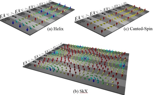
Figure 1: Schematics of three typical magnetic states in a thin film where the anisotropy exhibits periodic spatial variation of easy axis (EA) from in-plane (denoted by $\leftrightarrow$) to out-of-plane (denoted by $\odot\otimes$).

II Ginzburg-Landau model

We assume that the film lies in the $x-y$ plane, and that the film thickness is sufficiently thin so that the magnetization density $\mathbf{M}$ is uniform along the $z$-direction and hence is a function only of $x$ and $y$, i.e., $\mathbf{M=M}\left(x,y\right)$. In the GL theory, the spatial average of the total magnetic free energy ${\cal F}_{tot}$ of a ferromagnetic thin film of area $S$ may be written as

$$\mathcal{F}_{tot}=S^{-1}\int \mathrm{d}^{2}\mathbf{x}\left[A_{ex}\left(\nabla\mathbf{m}\right)^{2}+t\mathbf{m}^{2}+u\left(\mathbf{m}^{2}\right)^{2}\right.$$

$$\left.-\mu_{0}\mathbf{m\cdot H}M_{0}+K_{d}m_{z}^{2}+f_{a}\left(\mathbf{m}\right)\right]\,,$$ (1)

where $\mathbf{m=M}/M_{0}$ with $|{\mathbf{M}}|=M(T)$ the local magnetization density at temperature $T$ and $M_{0}=|{\mathbf{M}}|(T\to 0)$, $t$ and $u$ are GL parameters that are in general functions of temperature and external magnetic field, $\mu_{0}$ is the magnetic permeability, and $K_{d}m_{z}^{2}=\frac{1}{2}\mu_{0}M_{0}^{2}m_{z}^{2}$ denotes the demagnetizing energy density in the thin film approximation Harte (1968). We shall draw particular attention to the anisotropy energy density $f_{a}\left(\mathbf{m}\right)$. The uniaxial magnetic anisotropy with spatially varying easy axis may be modeled as

$$f_{a}\left[\mathbf{m}\left(\mathbf{x}\right)\right]=-K_{u}\left[\varkappa_{+}\left(x\right)m_{z}^{2}+\varkappa_{-}\left(x\right)m_{y}^{2}\right]\,,$$ (2)

where $\varkappa_{\pm}(x)\equiv\frac{1}{2}\left[\left|\cos\left(\frac{\pi x}{w_{t}}\right)\right|\pm\cos\left(\frac{\pi x}{w_{t}}\right)\right]$ with $w_{t}$ is the twin width, and $K_{u}\left(>0\right)$ characterizes the magnitude of the anisotropy.

A generalized spatial profile of the magnetization of a skyrmion lattice can be approximated as a superposition of three spin helices Mühlbauer et al. (2009); Nagaosa and Tokura (2013)

$$\mathbf{m}\left(\mathbf{r}\right)= \left[m_{0}+m_{i,\perp}\cos\left(\mathbf{k}_{i}\cdot\mathbf{r}\right)\right]\,\hat{\mathbf{z}}$$

$$+m_{i,\parallel}\left(\hat{\mathbf{z}}\times\mathbf{\hat{k}}_{i}\right)\sin\left(\mathbf{k}_{i}\cdot\mathbf{r}\right)\,,$$ (3)

where $m_{0}$ is the uniform magnetization induced by the external magnetic field perpendicular to the film plane, $m_{i,\perp}$ and $m_{i,\parallel}$ are the out-of-plane and in-plane components of the magnetization, and we use Einstein’s summation convention over repeated indices. The wave vectors of the three helices are all in the plane of the layer and form an angle of $120^{\circ}$ with each other; explicitly, we choose $\mathbf{k}_{1}=q\hat{\mathbf{x}}$, $\mathbf{k}_{2}=\left(-\frac{1}{2}\hat{\mathbf{x}}+\frac{\sqrt{3}}{2}\hat{\mathbf{y}}\right)q$ and $\mathbf{k}_{3}=\left(-\frac{1}{2}\hat{\mathbf{x}}-\frac{\sqrt{3}}{2}\hat{\mathbf{y}}\right)q$, and $\mathbf{\hat{k}}_{i}=\mathbf{k}_{i}/\left|\mathbf{k}_{i}\right|$ is the unit vector of $\mathbf{k}_{i}$. The general spatial profile given by Eq. (3) can be reduced to multiple magnetic states including: (i) Helix (single-$\mathbf{q}$ state) when $m_{1,\parallel}\approx m_{1,\perp}\neq 0$ and $m_{i,\parallel}=m_{i,\perp}=0$ ($i=2,3$); (ii) Stripe domain when only $m_{1,\perp}$ is nonzero; (iii) (nonchiral) bubble lattice when $m_{i,\perp}\neq 0$ and $m_{i,\parallel}=0$ ($i=1,2,3$); (iv) SkX (triple-$\mathbf{q}$ state) when $m_{i,\parallel}\approx m_{i,\perp}\neq 0$ and $m_{i,\perp}m_{i,\parallel}$ ($i=1,2,3$) have the same sign so that the three superimposed helices exhibit the same chirality. Other magnetic states are possible as we will mention below.

To simplify the problem without loss of generality, we shall assume that the magnitude of the magnetization has mirror symmetry about the $y=0$ plane, and let $m_{2,\perp}=m_{3,\perp}\text{, and }m_{2,\parallel}=m_{3,\parallel}\,.$ By placing Eq. (3) in Eq. (1) and carrying out the integration in Eq. (1), one can obtain the spatially averaged free energy density. The expression for this is complicated and not very instructive, and is given in the supplementary material.

The global minimum of the magnetic free energy density can be computed with the following six variational parameters: $m_{0},m_{1,\parallel},m_{2,\parallel}$, $m_{1,\perp}$, $m_{2,\perp}$ and $q$. To specify the two GL parameters $t$ and $u$, we introduce an extra positive definite free energy density term that arises when the magnetization density deviates from its uniform bulk saturation value $M_{s}$ Wang and Zhang (2013); Landis (2008), i.e., $\delta f=\chi\left(\mathbf{m}^{2}-\mathbf{m}_{s}^{2}\right)^{2}\,.$ Here, $\chi$ is a positive definite parameter which in principle relies on the magnetic property of the material, and the reduced saturation magnetization $m_{s}(\equiv M_{s}/M_{0})$ can be determined by self-consistently solving the equation $M_{s}=M_{0}B_{S}\left(T,H_{z}\right)$ in the mean field approximation with $B_{S}\left(T,H_{z}\right)$ the Brillouin function. We thus identify $t=-2\chi m_{s}^{2}$ and $u=\chi$. Just below $T_{c}$, the mean field equation gives $m_{s}\sim(1-\frac{T}{T_{c}})^{1/2}$, by which one recovers $t=k_{B}\left(T-T_{c}\right)/2v_{0}$ in the case of a 1-D Ising ferromagnet Garel and Doniach (1982) when $\chi=k_{B}T_{c}/4v_{0}$. We also impose the constraint that the spatially averaged magnetization modulus be no greater than the saturation magnetization, i.e., $S^{-1}\int d^{2}\mathbf{r}\left|\mathbf{m}\right|^{2}\leq m_{s}^{2}$.

III Results and discussion

In Fig. 2, we show the phase diagram in the temperature-field plane, where the field is applied out-of-plane, for several different magnitude of the demagnetizing and anisotropy energy density coefficients, i.e., $K_{d}$ and $K_{u}$. We note that in the absence of uniaxial anisotropy, only the uninteresting uniform magnetized state is observed (not shown). Once the anisotropy is turned on, the helix state prevails at low magnetic fields because of the alternating in-plane and out-of-plane easy axis variants. When the out-of-plane magnetic field $H_{z}$ increases, the negative $z$-component of the magnetization diminishes in a manner such that magnetizations with an out-of-plane component start to swirl around in order to lower the exchange energy, similar to the case in chiral magnets Nagaosa and Tokura (2013). This gives birth to the SkX phase as seen in Figs 2 (a) and (b). We also note that, for a given magnitude of the anisotropy, the SkX phase region is more extended for larger $K_{d}$ since then a greater magnetic field is needed to overcome the demagnetizing field. Further increasing the magnetic field leads to the canted-spin state with a large out-of-plane magnetization component parallel to the magnetic field together with small in-plane magnetization components forming an antiferromagnetic arrangement along the $x$-axis. Also, for a given magnitude of the magnetistatic energy $K_{d}$, a larger anisotropy lowers the energy barrier between the helix and canted-spin states and hence makes the SkX phase unstable, as indicated in Figs. 2 (a) and (c).

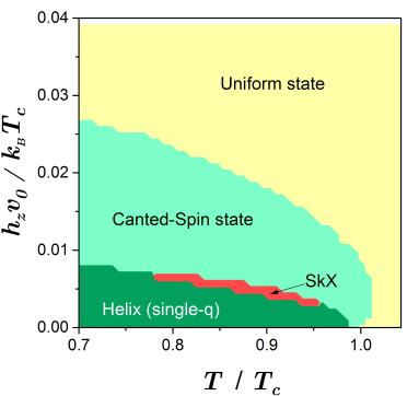
(a)  $K_{u}=K_{u0}$ & $K_{d}=K_{d0}$

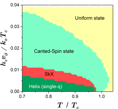
(b)  $K_{u}=K_{u0}$ & $K_{d}=1.5~{}K_{d0}$

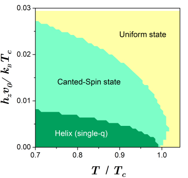
(c)  $K_{u}=1.5~{}K_{u0}$ & $K_{d}=K_{d0}$

Figure 2: Phase diagram in the plane of the out-of-plane magnetic field $h_{z}(\equiv M_{0}H_{z})$ and temperature $T$. Material parameters used in the calculation (corresponding to Ni₂MnGa Tickle and James (1999); Heczko et al. (2001); Wu et al. (2011); Sakon et al. (2013)): $A_{ex}=1.0\times 10^{-11}$ $J/m$, $M_{0}=6.0\times 10^{5}$ A/m, $K_{u0}=2.5\times 10^{5}$ J/m³ and $w_{t}=50$ nm. Small variations in the parameters may change the phase boundary, but the topology of the phase diagrams remains the same.

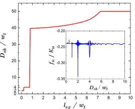
Figure 3: Skyrmion diameter as a function of exchange length for a thin film with total of 50 twin variants, i.e., $N_{t}=50$ and fixed width of twin width of $w_{t}=50~{}nm$. The inset shows the coefficient of anisotropy energy density $f_{u}$ as a function of the diameter of a skyrmion $D_{sk}(=\frac{2\pi}{q})$.

Next, we show that the the size of the skyrmions depends strongly on the magnitude of the anisotropy as well as on the width of the twin variant. In order to see this, let us focus on the free energy density of a standard SkX state given by

$$\bar{f}_{sk}\left(q\right)= \left(t+K_{d}-\pi^{-1}K_{u}\right)m_{0}^{2}+um_{0}^{4}-h_{z}m_{0}$$

$$+ \frac{1}{4\pi}\left[f_{ex}\left(q\right)+f_{u}\left(q\right)+48um_{0}^{2}+6\pi K_{d}\right]m_{sk}^{2}$$

$$+9um_{0}m_{sk}^{3}+\frac{51}{4}um_{sk}^{4}\,,$$ (4)

where we have set $m_{i,\parallel}=m_{i,\perp}$ $=m_{sk}$ ($i=1,2,3$) in Eq. (3). The $q$-dependence of the free energy enters through the coefficients of the exchange and anisotropy energy densities given by $f_{ex}\left(q\right)=12\pi A_{ex}q^{2}$ and

$$f_{u}\left(q\right)=-K_{u} \left[9-2\zeta_{N_{t}}\left(2w_{t}q\right)+2\eta_{N_{t}}\left(2w_{t}q\right)\right.$$

$$\left.-\zeta_{N_{t}}\left(w_{t}q\right)+4\eta_{N_{t}}\left(w_{t}q\right)\right]\,,$$ (5)

respectively, where $\eta_{N_{t}}\left(x\right)\equiv\frac{\sin\left[\left(N_{t}-1\right)x\right]+\sin\left(x\right)}{4N_{t}\left[1-(\frac{x}{\pi})^{2}\right]\sin\left(\frac{x}{2}\right)}$ and $\zeta_{N_{t}}\left(x\right)\equiv\frac{\sin\left[N_{t}x\right]}{4N_{t}\left[1-(\frac{x}{\pi})^{2}\right]\sin\left(\frac{x}{2}\right)}$ with $N_{t}$ the total number of twin variants which is taken to be an even number without loss of generality [see the supplementary material for a detailed derivation of $f_{u}(q)$].

The diameter of a skyrmion can thus be determined via $D_{sk}=\frac{2\pi}{q_{m}}$, where $q_{m}$ is the wave vector obtained by minimizing $f_{q}=f_{ex}+f_{u}$. In Fig. 3, we show $D_{sk}$ as a function of the exchange length $l_{ex}=2\pi\sqrt{\frac{A_{ex}}{K_{u}}}$ which is the length scale of a $360^{\circ}$ Bloch domain. When $l_{ex}$ is greater than the width of the twin $w_{t}$ (corresponding to small anisotropy $K_{u}$ for fixed exchange stiffness), the size of the skyrmion is comparable to and eventually approaches the lateral size of the film (i.e., $L=N_{t}w_{t}=2.5$ $\mu m$ for $N_{t}=50$ and $w_{t}=50$ $nm$); in other words, the system is essentially in a uniformly magnetized state in the small anisotropy regime. In the intermediate anisotropy regime where $l_{ex}\lesssim w_{t}$, a plateau of $D_{sk}=4w_{t}$ appears, which agrees with the experimental observation of the the close-packed hexagonal skyrmion lattice in the narrow twinned region of Ni₂MnGa. Finally, in the large anisotropy limit where the exchange length is much smaller than the twin width, another plateau of $D_{sk}=2w_{t}$ appears. These two plateaus result from the two local minimum in the anisotropy density characterized by the function $f_{u}$ given by Eq. (5) at $D_{sk}=2w_{t}$ and $D_{sk}=4w_{t}$, as shown by the inset of the Fig. 3.

Before we close this section, we briefly discuss the chirality and magnetic field dependence of the SkX. It was observed experimentally that the Ni₂MnGa crystal with inversion symmetry (and thus no DMI) still may host a SkX with a single chirality, in contrast to the SkX stabilized by long range dipolar interaction for which the chirality of each individual skyrmion could in principle be completely random. By adopting our Ansatz magnetization profile, we presumed all skyrmions have the same chirality, but our analysis provides several hints about the origin of the fixed chirality of the SkX in this system. First, as shown in the phase diagram (Fig. 2), the helix state is favored at low magnetic fields. Continuous transition from the helix state to SkX state necessitates a single chirality of the SkX even in the absence of the DMI, since the in-plane magnetization orientation must conform to that of the helix in order to lower the exchange energy cost during the transition. Second, as the separation distance between two neighboring skyrmions becomes shorter, same chirality becomes energetically preferable considering that the in-plane magnetization component along a line connecting the centers of the two skyrmions with opposite chiralities would carry higher order harmonics and thus results in higher exchange energy.

We finally comment on the dependence of the stability of the SkX hosted in the Ni₂MnGa system on the external magnetic field. Based on our theoretical model, a small but finite magnetic field is required to overcome the demagnetizing field and stabilizing the SkX phase; the magnetic field is of the order of $50$ $Oe$ as estimated for an Ni₂MnGa ultrathin film of 10 monolayers at room temperature, where $h_{z}v_{0}/k_{B}T_{c}\simeq 0.05$, $v_{0}=a_{m}^{2}d$ with the magnetic spacing $a_{m}\sim 10~{}\mathring{A}$ Righi et al. (2007); Sakon et al. (2013) and $d$ the thickness. Experimentally, SkX was observed even in the absence of external magnetic field Phatak et al. (2016). The observed (metastable) zero-field SkX may arise from the history-dependence of the system, e.g., a quenched SkX. Furthermore, we note that Ni₂MnGa is a ferromagnetic shape memory alloy, and there is a strain energy and an associated internal magnetic field induced by the magneto-elastic coupling involved in the martensite transformation; this is not considered explicitly in our present model, but would be interesting for future studies, as stabilization of skyrmions with zero magnetic field will be beneficial for the application of skyrmions in future electronic devices.

IV Summary and outlook

In this work, we generalized the Ginzburg-Landau theory for Ising ferromagnets to include a general continuum magnetization profile that encapsulates various magnetic configurations with three dimensional magnetization directions. We demonstrated that stabilization of room temperature SkX can be facilitated by geometric modulation of the uniaxial anisotropy easy axis in nonchiral materials with inversion symmetry. Remarkably, the size of the skyrmions can be tailored by the period of the spatial modulation of the anisotropy, in contrast with skyrmions originating from dipolar interaction and DMI. Such novel uniaxial anisotropy was realized experimentally in a multiferroic material Ni₂MnGa with narrow twin variants for which the anisotropy easy axis is rotated by $90^{\circ}$ across the twin boundary, and our work explains the underlying physics that gives rise to the observed SkX in Ni₂MnGa.

Our model can be further generalized to take into account other magnetic interactions such as the DMI as well as various forms of geometric confinement on magnetic structures. It will also be very intriguing to investigate the transport and dynamic behaviors of skyrmions in the presence of geometric modulation of the anisotropy. For example, with the nonuniform anisotropy that we considered here, one would expect the skyrmions to respond rather differently when they are driven along and perpendicular to the twin boundaries. It may also be possible to control and alter the chirality of the SkX using, e.g., strain or electrical currents. These centrosymmetric SkXs may therefore enable interesting applications in spintronics.

Appendix A General expression of the spatially averaged free energy density

By placing the general magnetization profile (Eq. (3) in the main text) in the magnetic free energy expression given by Eq. (1) in the main text, we obtain the following spatially average free energy density

$$\bar{f} =\left(t+K_{d}-\pi^{-1}K_{u}\right)m_{0}^{2}+um_{0}^{4}-h_{z}m_{0}$$

$$+\frac{1}{2\pi}\left\{\pi\left(A_{ex}q^{2}+t+2um_{0}^{2}\right)-K_{u}\left[1-\zeta_{N_{t}}\left(2w_{t}q\right)\right]\right\}m_{1,\parallel}^{2}$$

$$+\frac{1}{2\pi}\left\{\pi\left(A_{ex}q^{2}+t+6um_{0}^{2}+K_{d}\right)-K_{u}\left[1+\eta_{N_{t}}\left(2w_{t}q\right)\right]\right\}m_{1,\perp}^{2}$$

$$+\frac{1}{4\pi}\left\{4\pi\left(A_{ex}q^{2}+t+2um_{0}^{2}\right)-K_{u}\left[1-\zeta_{N_{t}}\left(w_{t}q\right)\right]\right\}m_{2,\parallel}^{2}$$

$$+\frac{1}{\pi}\left\{\pi\left(A_{ex}q^{2}+t+6um_{0}^{2}+K_{d}\right)-K_{u}\left[1+\eta_{N_{t}}\left(w_{t}q\right)\right]\right\}m_{2,\perp}^{2}$$

$$+um_{0}\left[2m_{1,\parallel}m_{2,\parallel}m_{2,\perp}+m_{1,\perp}\left(m_{2,\parallel}^{2}+6m_{2,\perp}^{2}\right)\right]$$

$$+\frac{u}{8}\left[3m_{1,\parallel}^{4}+3m_{1,\perp}^{4}+2m_{1,\parallel}^{2}m_{1,\perp}^{2}+12m_{2,\parallel}^{4}+18m_{2,\perp}^{4}+12m_{2,\parallel}^{2}m_{2,\perp}^{2}\right.$$

$$\left.+\text{ }12\left(m_{1,\parallel}^{2}m_{2,\parallel}^{2}+2m_{1,\perp}^{2}m_{2,\perp}^{2}\right)+8\left(m_{2,\parallel}^{2}m_{1,\perp}^{2}+m_{2,\perp}^{2}m_{1,\parallel}^{2}\right)\right]\,.$$ (A1)

where $h_{z}=M_{0}H_{z}$, and we have assumed, for simplicity without losing generality, that the magnitude of the magnetization has mirror symmetry about the $y=0$ plane, and let $m_{2,\perp}=m_{3,\perp}\text{, and }m_{2,\parallel}=m_{3,\parallel}$; the two functions $\eta_{N_{t}}\left(w_{t}q\right)$ and $\zeta_{N_{t}}\left(w_{t}q\right)$, with $N_{t}$ the total number of twin layers, are derived from the spatial integral of the anisotropy energy density. We will present the detailed derivation of the anisotropy free energy density term in the next section.

Appendix B Derivation of the anisotropy free energy density term

Let us consider the uniaxial magnetic anisotropy of the form

$$f_{a}\left[\mathbf{m}\left(\mathbf{x}\right)\right]=-K_{\perp}\left(x\right)m_{z}^{2}-K_{\parallel}\left(x\right)m_{x}^{2}$$ (A2)

with

$$K_{\perp}\left(x\right)=\frac{1}{2}K_{u}\left[\cos\left(\frac{\pi x}{w_{t}}\right)+\left|\cos\left(\frac{\pi x}{w_{t}}\right)\right|\right]$$ (A3)

and

$$K_{\parallel}\left(x\right)=\frac{1}{2}K_{u}\left[\left|\cos\left(\frac{\pi x}{w_{t}}\right)\right|-\cos\left(\frac{\pi x}{w_{t}}\right)\right]\,,$$ (A4)

where the prefactor $K_{u}$ measures the magnitude of the anisotropy energy density, $w_{t}$ is the period of the spatial variation of the anisotropy (or the width of the twin).

For the interesting case of $q>\pi/L$ with $L$ the side length of the rectangular film, the spatially averaged anisotropy energy can be calculated by the following piece-wise integration

$$\bar{f}_{a}=-\frac{\sqrt{3}q}{4\pi}\int_{-\frac{2\pi}{\sqrt{3}q}}^{\frac{2\pi}{\sqrt{3}q}}dy\sum_{n=0}^{N_{t}/2-1}\frac{K_{u}}{N_{t}w_{t}}\left[\int_{\left(2n-\frac{1}{2}\right)w_{t}}^{\left(2n+\frac{1}{2}\right)w_{t}}dx\cos\left(\frac{\pi x}{w_{t}}\right)m_{z}^{2}-\int_{\left(2n+\frac{1}{2}\right)w_{t}}^{\left(2n+\frac{3}{2}\right)w_{t}}dx\cos\left(\frac{\pi x}{w_{t}}\right)m_{y}^{2}\right]\,,$$ (A5)

where we have assumed $N_{t}$ being an large even integer number. By carrying out the integration, we obtain

$$\bar{f}_{a}=-\frac{K_{u}}{4\pi N_{t}}\sum_{n=0}^{N_{t}/2-1} \left\{2\left(4m_{0}^{2}+2m_{1,\perp}^{2}+4m_{2,\perp}^{2}+2m_{1,\parallel}^{2}+m_{2,\parallel}^{2}\right)+\frac{2m_{1,\parallel}^{2}b_{n}\left(2w_{t}q\right)}{\left(\frac{2w_{t}q}{\pi}\right)^{2}-1}-\frac{m_{2,\parallel}^{2}b_{n}\left(w_{t}q\right)}{1-\left(\frac{w_{t}q}{\pi}\right)^{2}}\right.$$

$$\left.-2\left[\frac{\left(4m_{0}m_{1,\perp}+2m_{2,\perp}^{2}\right)a_{n}\left(w_{t}q\right)}{\left(\frac{w_{t}q}{\pi}\right)^{2}-1}+\frac{m_{1,\perp}^{2}a_{n}\left(2w_{t}q\right)}{\left(\frac{2w_{t}q}{\pi}\right)^{2}-1}\right]\right\}\,,$$ (A6)

where $a_{n}\left(x\right)=\cos\left(2nx\right)\cos\left(\frac{x}{2}\right)$ and $b_{n}\left(x\right)=\cos\left[\left(2n+1\right)x\right]\cos\left(\frac{x}{2}\right)$, and the results of the summation of corresponding series are given as follows

$$\sum_{n=0}^{l}a_{n}\left(x\right)=\cos\left(\frac{x}{2}\right)\csc\left(w_{t}q\right)\cos\left(lw_{t}q\right)\sin\left[\left(l+1\right)w_{t}q\right]$$ (A7)

and

$$\sum_{n=0}^{l}b_{n}\left(x\right)=\sum_{n=0}^{l}\cos\left[\left(2n+1\right)x\right]\cos\left(x/2\right)=\cos\left(\frac{x}{2}\right)\csc\left(x\right)\cos\left[\left(l+1\right)x\right]\sin\left[\left(l+1\right)x\right]\,.$$ (A8)

Placing Eqs. (A7) and (A8) in Eq. (A6), we obtain

$$\bar{f}_{a} =-\frac{K_{u}}{4\pi}\left\{4m_{0}^{2}+2m_{1,\perp}^{2}\left[1+\eta_{N_{t}}\left(2w_{t}q\right)\right]+4m_{2,\perp}^{2}\left[1+\eta_{N_{t}}\left(w_{t}q\right)\right]\right.$$

$$\left.+2m_{1,\parallel}^{2}\left[1-\zeta_{N_{t}}\left(2w_{t}q\right)\right]+m_{2,\parallel}^{2}\left[1-\zeta_{N_{t}}\left(w_{t}q\right)\right]-8m_{0}m_{1,\perp}\zeta_{N_{t}}\left(w_{t}q\right)\right\}\,,$$ (A9)

where

$$\zeta_{N_{t}}\left(w_{t}q\right)=\frac{\pi^{2}\sin\left(N_{t}w_{t}q\right)}{4N_{t}\left(\pi^{2}-q^{2}w_{t}^{2}\right)\sin\left(\frac{w_{t}q}{2}\right)}$$ (A10)

and

$$\eta_{N_{t}}\left(w_{t}q\right)=\pi^{2}\frac{\sin\left[\left(N_{t}-1\right)w_{t}q\right]+\sin\left(w_{t}q\right)}{4N_{t}\left(\pi^{2}-q^{2}w_{t}^{2}\right)\sin\left(\frac{w_{t}q}{2}\right)}\,.$$ (A11)

Note that $\left|\zeta_{N_{t}}\left(x\right)\right|\leq\frac{1}{2}$ and $\left|\eta_{N_{t}}\left(x\right)\right|\leq\frac{1}{2}$, and the cross-term of $m_{0}m_{1,\perp}$ in Eq. (A9) vanishes when one carries out the spatial integration with an overall sinusoidal envelop function with the period of the film length on top of the magnetization profile [corresponding to several replica of the entire thin film]. Taking this into account, we arrive at the final expression of the anisotropy energy density in the presence of the geometric confinement with only quadratic terms, i.e.,

$$\bar{f}_{a} =-\frac{K_{u}}{4\pi}\left\{4m_{0}^{2}+2m_{1,\perp}^{2}\left[1+\eta_{N_{t}}\left(2w_{t}q\right)\right]+4m_{2,\perp}^{2}\left[1+\eta_{N_{t}}\left(w_{t}q\right)\right]\right.$$

$$\left.+2m_{1,\parallel}^{2}\left[1-\zeta_{N_{t}}\left(2w_{t}q\right)\right]+m_{2,\parallel}^{2}\left[1-\zeta_{N_{t}}\left(w_{t}q\right)\right]\right\}\,.$$ (A12)

The above expression is valid when $q>\pi/L_{i}$, where $L_{i}$ ($i=x$ or $y$) are side lengths of the rectangular thin film.

References

- Fert et al. (2017) A. Fert, N. Reyren, and V. Cros, Nat. Rev. Mater. 2, 17031 (2017).
- Mühlbauer et al. (2009) S. Mühlbauer, B. Binz, F. Jonietz, C. Pfleiderer, A. Rosch, A. Neubauer, R. Georgii, and P. Böni, Science 323, 915 (2009).
- Nagaosa and Tokura (2013) N. Nagaosa and Y. Tokura, Nat Nano 8, 899 (2013).
- Hellman et al. (2017) F. Hellman, A. Hoffmann, Y. Tserkovnyak, G. S. D. Beach, E. E. Fullerton, C. Leighton, A. H. MacDonald, D. C. Ralph, D. A. Arena, H. A. Dürr, P. Fischer, J. Grollier, J. P. Heremans, T. Jungwirth, A. V. Kimel, B. Koopmans, I. N. Krivorotov, S. J. May, A. K. Petford-Long, J. M. Rondinelli, N. Samarth, I. K. Schuller, A. N. Slavin, M. D. Stiles, O. Tchernyshyov, A. Thiaville, and B. L. Zink, Rev. Mod. Phys. 89, 025006 (2017).
- Rohart et al. (2016) S. Rohart, J. Miltat, and A. Thiaville, Phys. Rev. B 93, 214412 (2016).
- Okubo et al. (2012) T. Okubo, S. Chung, and H. Kawamura, Phys. Rev. Lett. 108, 017206 (2012).
- Heinze et al. (2011) S. Heinze, K. von Bergmann, M. Menzel, J. Brede, A. Kubetzka, R. Wiesendanger, G. Bihlmayer, and S. Blugel, Nat Phys 7, 713 (2011).
- Jiang et al. (2015) W. Jiang, P. Upadhyaya, W. Zhang, G. Yu, M. B. Jungfleisch, F. Y. Fradin, J. E. Pearson, Y. Tserkovnyak, K. L. Wang, O. Heinonen, S. G. E. te Velthuis, and A. Hoffmann, Science 349, 283 (2015).
- Heinonen et al. (2016) O. Heinonen, W. Jiang, H. Somaily, S. G. E. te Velthuis, and A. Hoffmann, Phys. Rev. B 93, 094407 (2016).
- Woo et al. (2016) S. Woo, K. Litzius, B. Kruger, M.-Y. Im, L. Caretta, K. Richter, M. Mann, A. Krone, R. M. Reeve, M. Weigand, P. Agrawal, I. Lemesh, M.-A. Mawass, P. Fischer, M. Klaui, and G. S. D. Beach, Nat Mater 15, 501 (2016).
- Boulle et al. (2016) O. Boulle, J. Vogel, H. Yang, S. Pizzini, D. de Souza Chaves, A. Locatelli, T. O. Mentes, A. Sala, L. D. Buda-Prejbeanu, O. Klein, M. Belmeguenai, Y. Roussigné, A. Stashkevich, S. M. Chérif, L. Aballe, M. Foerster, M. Chshiev, S. Auffret, I. M. Miron, and G. Gaudin, Nat Nano 11, 449 (2016).
- Zhang et al. (2016) S. Zhang, A. K. Petford-Long, and C. Phatak, Sci. Rep. 6, 31248 (2016).
- Lin et al. (1973) Y. S. Lin, P. J. Grundy, and E. A. Giess, Appl. Phys. Lett. 23, 485 (1973), http://dx.doi.org/10.1063/1.1654968 .
- Takao (1983) S. Takao, J. Magn. Magn. Mater. 31, 1009 (1983).
- Malozemoff and Slonczewski (1979) A. P. Malozemoff and J. C. Slonczewski, Magnetic Domain Walls in Bubble Materials, edited by R. Wolfe (Academic Press, 1979).
- Lebech et al. (1995) B. Lebech, P. Harris, J. S. Pedersen, K. Mortensen, C. Gregory, N. Bernhoeft, M. Jermy, and S. Brown, J. Magn. Magn. Mater. 140, 119 (1995).
- Bauer and Pfleiderer (2012a) A. Bauer and C. Pfleiderer, Phys. Rev. B 85, 214418 (2012a).
- Grigoriev et al. (2009) S. V. Grigoriev, D. Chernyshov, V. A. Dyadkin, V. Dmitriev, S. V. Maleyev, E. V. Moskvin, D. Menzel, J. Schoenes, and H. Eckerlebe, Phys. Rev. Lett. 102, 037204 (2009).
- Uchida et al. (2008) M. Uchida, N. Nagaosa, J. P. He, Y. Kaneko, S. Iguchi, Y. Matsui, and Y. Tokura, Phys. Rev. B 77, 184402 (2008).
- Yu et al. (2011) X. Z. Yu, N. Kanazawa, Y. Onose, K. Kimoto, W. Z. Zhang, S. Ishiwata, Y. Matsui, and Y. Tokura, Nat Mater 10, 106 (2011).
- Wilhelm et al. (2011) H. Wilhelm, M. Baenitz, M. Schmidt, U. K. Rößler, A. A. Leonov, and A. N. Bogdanov, Phys. Rev. Lett. 107, 127203 (2011).
- Shibata et al. (2013) K. Shibata, Z. X. Yu, T. Hara, D. Morikawa, N. Kanazawa, K. Kimoto, S. Ishiwata, Y. Matsui, and Y. Tokura, Nat Nano 8, 723 (2013).
- Dzyaloshinsky (1958) I. Dzyaloshinsky, J Phys Chem Solids 4, 241 (1958).
- Moriya (1960) T. Moriya, Phys. Rev. 120, 91 (1960).
- Emori et al. (2013) S. Emori, U. Bauer, S.-M. Ahn, E. Martinez, and G. S. D. Beach, Nat Mater 12, 611 (2013).
- Ryu et al. (2013) K.-S. Ryu, L. Thomas, S.-H. Yang, and S. Parkin, Nat Nano 8, 527 (2013).
- McMillan (1975) W. L. McMillan, Phys. Rev. B 12, 1187 (1975).
- Bocdanov and Hubert (1994) A. Bocdanov and A. Hubert, physica status solidi (b) 186, 527 (1994).
- Leonov et al. (2016) A. O. Leonov, T. L. Monchesky, N. Romming, A. Kubetzka, A. N. Bogdanov, and R. Wiesendanger, New J. Phys. 18, 065003 (2016).
- Bauer and Pfleiderer (2012b) A. Bauer and C. Pfleiderer, Phys. Rev. B 85, 214418 (2012b).
- Montoya et al. (2017a) S. A. Montoya, S. Couture, J. J. Chess, J. C. T. Lee, N. Kent, D. Henze, S. K. Sinha, M.-Y. Im, S. D. Kevan, P. Fischer, B. J. McMorran, V. Lomakin, S. Roy, and E. E. Fullerton, Phys. Rev. B 95, 024415 (2017a).
- Moreau-Luchaire et al. (2016) C. Moreau-Luchaire, C. Moutafis, N. Reyren, J. Sampaio, C. A. F. Vaz, N. Van Horne, K. Bouzehouane, K. Garcia, C. Deranlot, P. Warnicke, P. Wohlhüter, J.-M. George, M. Weigand, J. Raabe, V. Cros, and A. Fert, Nat Nano 11, 444 (2016).
- Jin et al. (2017) C. Jin, Z.-A. Li, A. Kovács, J. Caron, F. Zheng, F. N. Rybakov, N. S. Kiselev, H. Du, S. Blügel, M. Tian, Y. Zhang, M. Farle, and R. E. Dunin-Borkowski, Nat Commun 8, 15569 (2017).
- Montoya et al. (2017b) S. A. Montoya, S. Couture, J. J. Chess, J. C. T. Lee, N. Kent, D. Henze, S. K. Sinha, M.-Y. Im, S. D. Kevan, P. Fischer, B. J. McMorran, V. Lomakin, S. Roy, and E. E. Fullerton, Phys. Rev. B 95, 024415 (2017b).
- Seki et al. (2012) S. Seki, X. Z. Yu, S. Ishiwata, and Y. Tokura, Science 336, 198 (2012).
- Yu et al. (2012) X. Yu, M. Mostovoy, Y. Tokunaga, W. Zhang, K. Kimoto, Y. Matsui, Y. Kaneko, N. Nagaosa, and Y. Tokura, PNAS 109, 8856 (2012).
- Langner et al. (2014) M. C. Langner, S. Roy, S. K. Mishra, J. C. T. Lee, X. W. Shi, M. A. Hossain, Y.-D. Chuang, S. Seki, Y. Tokura, S. D. Kevan, and R. W. Schoenlein, Phys. Rev. Lett. 112, 167202 (2014).
- White et al. (2014) J. S. White, K. Prša, P. Huang, A. A. Omrani, I. Živković, M. Bartkowiak, H. Berger, A. Magrez, J. L. Gavilano, G. Nagy, J. Zang, and H. M. Rønnow, Phys. Rev. Lett. 113, 107203 (2014).
- Phatak et al. (2016) C. Phatak, O. Heinonen, M. D. Graef, and A. Petford-Long, Nano Lett. 16, 4141 (2016).
- Garel and Doniach (1982) T. Garel and S. Doniach, Phys. Rev. B 26, 325 (1982).
- Harte (1968) K. J. Harte, J. Appl. Phys. 39, 1503 (1968).
- Wang and Zhang (2013) J. Wang and J. Zhang, Int. J. Solids Struct. 50, 3597 (2013).
- Landis (2008) C. M. Landis, J. Mech. Phys. Solids 56, 3059 (2008).
- Tickle and James (1999) R. Tickle and R. James, J. Magn. Magn. Mater. 195, 627 (1999).
- Heczko et al. (2001) O. Heczko, K. Jurek, and K. Ullakko, J. Magn. Magn. Mater. 226, 996 (2001).
- Wu et al. (2011) P. Wu, X. Ma, J. Zhang, and L. Chen, Philos. Mag. 91, 2102 (2011).
- Sakon et al. (2013) T. Sakon, Y. Adachi, and T. Kanomata, Metals 3, 202 (2013).
- Righi et al. (2007) L. Righi, F. Albertini, L. Pareti, A. Paoluzi, and G. Calestani, Acta Mater. 55, 5237 (2007).