Alternative formulation of the macroscopic field equations in a linear magneto-dielectric medium: Lagrangian field theory and spacetime setting

Abstract

A transparent linear magneto-dielectric material in free space that is illuminated by a finite quasimonochromatic field is a thermodynamically closed system, definitively, regardless of what field and material subsystems that one defines. The energy–momentum tensor that is formally derived from the Maxwell–Minkowski field equations is inconsistent with both angular and linear momentum conservation in this closed system; this very solid fact is the foundational and continuing issue of the Abraham–Minkowski controversy. The extant resolution of the Abraham–Minkowski dilemma is to treat Maxwellian continuum electrodynamics as being a subsystem and to write the total energy–momentum tensor as the sum of a Maxwellian electromagnetic subsystem energy–momentum tensor and a phenomenological material subsystem energy–momentum tensor. We prove that fundamental principles of physics are violated by Maxwellian continuum electrodynamics and that fundamental principles of physics are violated by Maxwellian continuum electrodynamics supplemented by the material subsystem conjecture. We use field theory to derive legitimate equations for macroscopic electromagnetic fields in a transparent linear magneto-dielectric medium. The new field equations are a part of a self-consistent formulation of macroscopic electrodynamics, conservation laws, special relativity, and invariance in a continuous linear medium. In the new formulation, the temporal and spatial coordinates are renormalized by the continuous linear medium instead of the permittivity and permeability being carried as independent material parameters. Then an isotropic, homogeneous, flat, four-dimensional, continuous, linear, non-Minkowski spacetime is the proper setting for the continuum electrodynamics of a simple linear medium in which the effective speed of light is $c/n$ and each medium will be associated with a different spacetime.

I Introduction

Continuum electrodynamics can be defined as a formal theory whose axioms are the Maxwell–Minkowski equations (macroscopic Maxwell equations), the constitutive relations, and the definitions of the fields in terms of the vector potential. Theorems of continuum electrodynamics are formally generated by the operations of algebra and calculus on the axioms. In particular, the electromagnetic conservation law (see Eq. (15)) is a theorem of the Maxwell–Minkowski equations and constitutive relations in the limit that the gradient Minkowski four-force density is negligible. The formal derivation of the electromagnetic conservation law also derives the Minkowski energy–momentum tensor and the Minkowski momentum density.

We address a contradiction between the linear momentum conservation properties of two theorems of formal continuum electrodynamics; the electromagnetic conservation law and the wave equation. Specifically, the vanishing four-divergence of the Minkowski energy–momentum tensor for a quasimonochromatic field normally incident on a gradient-index antireflection coated transparent linear magneto-dielectric medium proves, via the (local) electromagnetic conservation law, that the Minkowski linear momentum is conserved [1, 2, 3, 4, 5], while global conservation analyses of the same system using the wave equation prove that the Minkowski linear momentum in the medium is greater than the vacuum-incident momentum by a factor of the refractive index $n$ [1, 6, 7, 8].

The formal theory is a precise axiomatic system and we must acknowledge that the disproof of a theorem of the formal theory, via contradiction between the electromagnetic conservation law and the wave equation, proves that the axioms, the macroscopic Maxwell–Minkowski equations, constitutive relations, and vector potential relations, are false. Instead, scientists assume that the model system is incomplete, ostensibly requiring the inclusion of a material-motion subsystem and a heuristic way to couple the phenomenological material subsystem to the electrodynamic subsystem in order to reconcile Maxwellian electrodynamic theory with the violated physical principles [9, 10, 1, 11, 12, 13, 6, 14, 15, 16, 17, 2].

The postulated incompleteness of the Minkowski energy–momentum tensor proves the incompleteness of the electromagnetic conservation law and thereby proves the incompleteness of the axioms from which the electromagnetic conservation law is derived as a theorem. Given that the electromagnetic conservation law, a formal theorem of the Maxwell-Minkowski field equations, results in long-known, scientifically reported [9, 10, 1, 11, 12, 13, 6, 14, 15, 16, 17, 2], and easily verified errors in the momentum, the question as to why the incomplete macroscopic Maxwell–Minkowski field equations are regarded as laws of physics, still, and continue to be treated as fundamental equations in textbooks and other scientific publications is a disturbing issue of scientific philosophy.

The foundational issue [18, 19] of the century-old Abraham–Minkowski controversy [9, 10, 1, 11, 12, 13, 6, 14, 15, 16, 17, 2] is that the non-symmetric Minkowski energy–momentum tensor is not consistent with conservation of angular momentum. Originally an issue of angular momentum conservation [18, 19], nowadays the Abraham–Minkowski controversy is typically characterized as a question about the physical meaning and usage of two different electromagnetic linear momentum formulas, the Minkowski electromagnetic momentum and the Abraham electromagnetic momentum, and the corresponding material subsystem momentums [9, 10, 1, 11, 12, 13, 6, 14, 15, 16, 17, 2, 20].

The ‘modern’ resolution of the Abraham–Minkowski controversy, reviewed in Sec. II, is to posit the existence of a material subsystem with a material subsystem energy–momentum tensor (or a material subsystem momentum) [9, 10, 1, 11, 12, 13, 6, 14, 15, 16, 17, 2]. The coupling between the electromagnetic and material subsystems is derived by global conservation of energy, global conservation of linear momentum, and conservation of angular momentum. Then we can write a total (field plus material) energy–momentum tensor (or the total momentum) [1, 21, 6, 14, 15]. Except, we prove that using the total (field plus material) energy–momentum tensor [1, 21] in the electromagnetic conservation law repairs global linear momentum conservation and angular momentum conservation, by hand, but violates other physical principles, i.e. relativity and the Poynting theorem, that are well-known to be satisfied by the Maxwell–Minkowski field equations. Then the conservation law is false without the material subsystem conjecture and it is false with the material subsystem conjecture.

Starting with Abraham [19] in 1909, manifold disproofs [9, 10, 1, 11, 12, 13, 6, 14, 15, 16, 17, 2] of the electromagnetic conservation law also disprove the Maxwell–Minkowski equations, the axioms from which the conservation law is formally constructed as a theorem that becomes an identity in the limit that a transient is neglected. Then the falsification of the Maxwell-Minkowski equations is a century-old matter of abstract algebra. Because the literature of the Abraham–Minkowski controversy contains a great amount of deflection about this point, we disprove several hypothetical resolutions of the issue in Sec. II, even though the disproof of the local electromagnetic conservation law is sufficient.

Minkowski spacetime is a model for the vacuum [22]. The spacetime conservation laws, Sec. III, are fundamental physical principles of Minkowski spacetime for the propagation of the unimpeded (no external forces), inviscid, incoherent, incompressible flow of non-interacting particles (nonpolar molecules, dust particles, or photons) in the continuum limit (fluid or light field (light fluid)) through an otherwise empty vacuum [23]. The conservation laws of Minkowski spacetime are fixed and immutable for any countable system obeying the specified conditions, for example, fluid flow in the vacuum or light flow in the vacuum. However, those laws change with physical circumstances. For example, the Navier–Stokes equation is a version of the spacetime conservation law that has been modified for a viscous flow through the otherwise empty vacuum.

Although the vacuum can be modeled as a Minkowski spacetime, we show that the effective medium description of a transparent simple linear magneto-dielectric medium in the continuum limit corresponds to a linear, isotropic, homogeneous, flat, four-dimensional, continuous non-Minkowski ‘material’ spacetime in which the effective speed of light is $c/n$. Because the unimpeded, inviscid, incoherent flow of a spatially compressed (compressed and de-compressed at the boundaries of the material, but not otherwise compressible) light field is traveling through a region of space that is not a vacuum, we must develop the physical laws that apply in the ‘material’ spacetime. The Maxwell–Minkowski equations are readily derived by using Lagrangian field theory in Minkowski spacetime [24, 25]. In Secs. IV and V, we develop field theory for a non-empty region of space that responds linearly to electromagnetic radiation with a speed of light $c/n$.

The current author performed a simple application of special relativity using inertial reference frames moving uniformly along the surface of a large transparent linear dielectric in Ref. [26]. It was shown that Einstein’s special relativity manifests differently for observers on opposite sides of the interface: i) An observer on the vacuum side of the interface uses boundary conditions to describe events that occur inside the dielectric using Laue’s [27] dielectric special relativity with a vacuum Lorentz factor and a velocity-dependent index of refraction. ii) An observer on the dielectric side of the interface finds that the application of Einstein’s relativity in a dielectric is best described by Rosen’s [28] dielectric special relativity in terms of a non-Lorentz (but Lorentz-like) factor that contains the permittivity of the dielectric and does not depend on the velocity of the dielectric. In Sec. VI, the derivation of Ref. [26] is applied to a simple linear magneto-dielectric medium and the result demonstrates that the Lorentz-like factor for the observer inside the continuous medium depends on the permittivity and permeability through the index of refraction. An observer inside an arbitrarily large continuous linear, isotropic, homogeneous, magneto-dielectric medium determines that the velocity of light $c/n$ is independent of the velocity of the source in accordance with the Principle of Relativity.

There are additional optical processes that need to be re-evaluated when they occur in a transparent, isotropic, homogeneous, continuous linear medium, instead of in the vacuum. In Sec. VII, we prove a linear, isotropic, homogeneous, flat, four-dimensional, continuous ‘material’ spacetime in which the temporal coordinate is normalized by the inverse of the square root of the permittivity and the spatial coordinates are normalized by the square root of the permeability. As has been known [29], Lorentz invariance is not of symmetry of a linear medium. In Sec. VIII, we establish a refractive-index-dependent invariance for the medium-dependent non-Minkowski spacetime of a continuous linear medium. This result implies that Laue’s theorem [30, 31] and Noether’s theorem [32] are re-defined for a simple linear medium by the new invariance principle, however, we focus on the more common electrodynamic principles and we do not derive these two theorems here. In Sec. IX, we construct a tensor formulation of continuum electrodynamics as theorems of the new field equations and note that the energy–momentum tensor is diagonally symmetric and that the electromagnetic energy and electromagnetic momentum are locally and globally conserved without the need for a material-motion subsystem. Finally, the new theory of continuum electrodynamics is shown to be consistent with the Balazs [33] thought experiment and the Jones–Richard [34] mirror experiment. It is shown that the uniform velocity of the center of mass-energy theorem depends on a constant mass-energy density. When applied to light propagation, the uniform velocity of the center of mass-energy theorem [34] must be modified to account for the change in the volume occupied by the energy and momentum of the field that is accompanied by the corresponding change in the energy and momentum density, Sec. X.

II Continuum Electrodynamics

The model system consists of a finite quasimonochromatic electromagnetic field and a block of simple linear magneto-dielectric material located in a large finite volume ${\Sigma}$ of free space. We define a simple linear medium as a transparent, isotropic, homogeneous, continuous linear medium that has no resonances near the center frequency of the quasimonochromatic field; the material is “effectively dispersionless at frequencies of interest” [10] (There is some ambiguity in the terminology used in the literature because dispersion is actually treated in lowest-order in the ‘dispersionless’ cases. The refractive index $n$ depends on the frequency of the field, but the frequency is treated as being constant for the duration of the quasimonochromatic field.) The material is initially at rest in the local frame. Unless the radiation is of extraordinary intensity and duration, the velocity of the material in the local frame will be non-relativistic and neglecting the effects of the material motion on the refractive index is an “extremely accurate approximation indeed” [17]. Then dispersion and velocity-dependence can be treated in lowest order such that the permittivity, permeability, and the refractive index can be represented by real constants. The values of these constants depend on the properties of the material and depend on the center frequency of the exciting quasimonochromatic field (dispersion is treated in lowest-order). The model system is the principal model of a simple linear medium that is extensively used in continuum electrodynamics, for example, the derivation of the Fresnel relations [35, 36, 37]. The stationary ‘dispersionless’ limit is implicitly and explicitly used in most lowest-order expositions of the Abraham–Minkowski controversy [10].

The electromagnetic theory is developed using vector and tensor formulations. For purposes of illustration, to compare magnitudes, for example, propagation of the field is discussed using the plane-wave limit. The plane-wave limit is a common abstraction with well-known characteristics that allows paraxial problems to be treated in lowest-order with one spatial dimension, not to be confused with the assumption of uniform plane waves that are nonphysical due to their infinite energy. The plane-wave limit is used in the typical derivation of the Fresnel relations and many other elementary problems of continuum electrodynamics [35, 36, 37]. The plane-wave limit is explicitly and implicitly used in many lowest-order expositions of the Abraham–Minkowski controversy.

The model quasimonochromatic field is initially in the vacuum and has a constant amplitude except for a short smooth turn-on transition and a short smooth turn-off transition. The field propagates toward and then enters the transparent, isotropic, homogeneous linear medium at normal incidence through a gradient-index antireflection coating. The field re-enters the vacuum through the gradient-index antireflection coating on the opposite side of the medium. The system, as defined, is obviously closed. In particular, any reflected field and whatever material motion that is imparted by the interaction with the field are part of the closed system along with the refracted and transmitted fields. Conservation laws can be applied to the thermodynamically closed system [2].

There is no scientific error in deriving theoretical results for a limiting case in a closed system. Once the theoretical results are derived for the limiting case (quasimonochromatic field, lowest-order dispersion, stationary medium, no sources or sinks, etc), the theory can be extended to more detailed models.

Brevik [2, 4] and Wang [5] use the vanishing four-divergence of the Minkowski energy–momentum tensor (see Eqs. (14a) and (15)) as a local conservation law [30] to prove that the Minkowski energy

$$U_{M}=\int_{\Sigma}\frac{{\bf D}\cdot{\bf E}+{\bf B}\cdot{\bf H}}{2}dv$$ (1)

and the Minkowski linear momentum

$${\bf G}_{M}=\int_{\Sigma}\frac{{\bf D}\times{\bf B}}{c}dv$$ (2)

form a Lorentz four-vector $(U_{M},{\bf G}_{M})$ in the limit that the Minkowski four-force density ${\bf f}^{\alpha}_{M}$ that is associated with the gradient-index antireflection coating can be neglected. This is considered to be a resolution of the Abraham–Minkowski controversy because the elements of a Lorentz four-vector are globally conserved [5, 30].

Except, that is not the case here. Although the Abraham–Minkowski dilemma was originally about conservation of angular momentum, it was well-known, almost from the outset of the controversy, that the Minkowski linear momentum ${\bf G}_{M}$ is not globally conserved [1, 7, 8, 6] thereby contradicting the determination [2, 4, 5] that $(U_{M},{\bf G}_{M})$ is a Lorentz four-vector.

That being said, it is common practice to dismiss the global conservation problem with the linear momentum by deeming the violation of global momentum conservation to be negligible based on the vanishing four-force density ${\bf f}^{\alpha}_{M}$ that appears as the right-hand side of the electromagnetic conservation law (see Eq. (14a)). Although the practice is scientifically countenanced by appealing to the electromagnetic conservation law (see Eq. (15)), the deduction contradicts the long–known, scientifically reported [1, 7, 8, 6] and easily verified fact that the Minkowski momentum in the material is the momentum of the field that is incident from the vacuum multiplied by a non-negligible factor of $n$.

A substantive contradiction exists between the (local) electromagnetic conservation law and the global conservation law. Adopting either the (local) electromagnetic conservation law or global conservation dictates the direction of the analysis and disproves the other. Although both aspects of the contradiction appear in the scientific literature, they typically appear separately thereby avoiding obvious contradictions. In their detailed, comprehensive review article, Pfeifer, Nieminen, Heckenberg, and Rubinsztein-Dunlop [1], present both sides of the issue but, due to the structure of a review article, the two results appear in different sections of the article with the global result of a factor of $n$ difference in the linear momentum being mentioned in Sec. III while the Minkowski momentum is described as (almost) conserved in Sec. VI-A in connection with the electromagnetic conservation law.

Next, we review the details of the argument using the familiar Maxwell–Minkowski formulation of macroscopic electrodynamics. Continuum electrodynamics can be described as a formal theory whose axioms are the Maxwell–Minkowski equations,

$$\nabla\times{\bf H}-\frac{\partial{\bf D}}{\partial(ct)}=\frac{{\bf J}_{f}}{c}$$ (3a)

$$\nabla\times{\bf E}+\frac{\partial{\bf B}}{\partial(ct)}=0$$ (3b)

$$\nabla\cdot{\bf D}=\rho_{f}$$ (3c)

$$\nabla\cdot{\bf B}=0\;,$$ (3d)

and constitutive relations,

$${\bf D}=\varepsilon{\bf E}$$ (4a)

$${\bf B}=\mu{\bf H}$$ (4b)

$$n=\sqrt{\varepsilon\mu}\;,$$ (4c)

for the macroscopic fields ${\bf E}$, ${\bf B}$, ${\bf D}$, and ${\bf H}$ in a simple linear magneto-dielectric medium. Later, the use of the wave equation will cause us to treat the relations between the vector potential ${\bf A}$ and the macroscopic fields (see Eqs. (17b)) as axioms, as well.

The free charge density $\rho_{f}$ and the free current density ${\bf J}_{f}$ are macroscopic parameters. Also, $\varepsilon$ is a continuum abstraction of the electric permittivity, $\mu$ is a continuum abstraction of the magnetic permeability, and $n$ is the macroscopic refractive index. The physical system, as we have defined it, allows us to treat the material parameters $\varepsilon$, $\mu$, and $n$ in lowest order as depending on the center frequency of the quasimonochromatic field but are otherwise single-valued real constants [35, 36, 37].

Describing the theoretical viewpoint of physics, Rindler [38] states “a physical theory is an abstract mathematical model (much like Euclidian geometry) whose applications to the real world consist of correspondences between a subset of it and a subset of the real world”. Continuum electrodynamics is constructed as a formal theory in this abstract mathematical framework by performing operations of algebra and calculus on the axioms. If any theorem of Eqs. (3d), (4c), and (17b) is proven false, then one or more of the axioms are proven false and all other theorems that are derived from the axioms are unproven.

Experimentalists [1, 20] have a different viewpoint and are concerned about including the full set of physical effects that might affect measurements because their experimental conditions are not usually as pristine as a theoretical model. Real-world effects, like damping, material motion, higher orders of dispersion, electrostriction, non-linearity, etc, can be important in a general setting, but these effects are obviously not going to fix the essential contradiction between the (local) electromagnetic conservation law and global conservation in the physical theory of the specified model system. Adding these higher-order effects to a provably flawed model is a meritless appeal to complexity in the face of a contradiction between theorems of the Maxwell–Minkowski equations. Those higher-order effects can be incorporated later to align the theory with experiments over a broad range of conditions once the contradiction is resolved.

Derivations of the electromagnetic momentum density continuity equation (momentum conservation law) typically begin with the Lorentz force law [10, 35, 36, 37]. The free charge momentum density ${\bf p}_{mech}$ imparted by the field to a distribution of free charges in the continuum limit can be calculated by postulating the Lorentz force density [10, 35, 36, 37]

$$\frac{d{\bf p}_{mech}}{dt}={\bf f}_{L}=\rho_{f}{\bf E}+\frac{{\bf J}_{f}}{c}\times{\bf B}$$ (5)

as a physical law [39, 40]. The sources are eliminated in favor of the fields using the Gauss law, Eq. (3c), to eliminate $\rho_{f}$ and using the Maxwell–Ampère law, Eq. (3a), to eliminate ${\bf J}_{f}$. Then the momentum density ${\bf p}_{mech}$ imparted to the free-charge density can be calculated by integrating [10, 35, 36, 37]

$$\rho_{f}{\bf E}+\frac{{\bf J}_{f}}{c}\times{\bf B}=(\nabla\cdot{\bf D}){\bf E}+\left(\nabla\times{\bf H}-\frac{1}{c}\frac{\partial{\bf D}}{\partial t}\right)\times{\bf B}\,.$$ (6)

Substituting the calculus identity

$$\frac{\partial}{\partial t}({\bf D}\times{\bf B})=\frac{\partial{\bf D}}{\partial t}\times{\bf B}+{\bf D}\times\frac{\partial{\bf B}}{\partial t}\,,$$ (7)

Faraday’s law, Eq. (3b), Thompson’s law, Eq. (3d), and Gauss’s law into Eq. (6) yields the momentum continuity equation [35, 36, 37]

$$\rho_{f}{\bf E}+\frac{{\bf J}_{f}}{c}\times{\bf B}=(\nabla\cdot{\bf D}){\bf E}+$$

$$(\nabla\cdot{\bf B}){\bf H}-{\bf D}\times(\nabla\times{\bf E})-{\bf B}\times(\nabla\times{\bf H})-\frac{1}{c}\frac{\partial}{\partial t}({\bf D}\times{\bf B})\,.$$ (8)

The textbook derivation is simple and the steps have obvious physical meaning. The textbook derivation is not as rigorous as we would like because we are unnecessarily postulating the Lorentz force density law, Eq. (5) [10, 35, 36, 37, 39, 40].

We propose an alternative derivation of the energy and momentum continuity equations as formal theorems of the Maxwell–Minkowski equations. We take the scalar product of Eq. (3b) with ${\bf H}$ and the scalar product of Eq. (3a) with ${\bf E}$ and subtract the results to produce a continuity equation [41, 42]

$$\frac{1}{c}\left({\bf E}\cdot\frac{\partial{\bf D}}{\partial t}+{\bf H}\cdot\frac{\partial{\bf B}}{\partial t}\right)+\nabla\cdot({\bf E}\times{\bf H})=-\frac{{\bf J}_{f}}{c}\cdot{\bf E}$$ (9)

that is a valid theorem (Poynting’s theorem) of the formal theory of continuum electrodynamics.

Adding the vector product of ${\bf B}$ with Eq. (3a), the vector product of ${\bf D}$ with Eq. (3b), the product of Eq. (3d) with $-{\bf H}$, and the product of Eq. (3c) with $-{\bf E}$ produces the momentum continuity equation

$$\frac{1}{c}\frac{\partial}{\partial t}({\bf D}\times{\bf B})+{\bf D}\times(\nabla\times{\bf E})+{\bf B}\times(\nabla\times{\bf H})$$

$$-(\nabla\cdot{\bf D}){\bf E}-(\nabla\cdot{\bf B}){\bf H}=-\rho_{f}{\bf E}-\frac{1}{c}{\bf J}_{f}\times{\bf B}$$ (10)

that is also a formal theorem of Maxwellian continuum electrodynamics [42].

The free charge density and the free charge current density are parameters that are determined by the specification of the system configuration. Then we can specify a system that consists of a neutral magneto-dielectric medium situated in the vacuum and illuminated by a finite quasimonochromatic field. The Maxwell–Minkowski equations, Eqs. (3d), become homogeneous Maxwell–Minkowski equations,

$$\nabla\times{\bf H}-\frac{\partial{\bf D}}{\partial(ct)}=0$$ (11a)

$$\nabla\times{\bf E}+\frac{\partial{\bf B}}{\partial(ct)}=0$$ (11b)

$$\nabla\cdot{\bf D}=0$$ (11c)

$$\nabla\cdot{\bf B}=0\;,$$ (11d)

for a neutral simple linear medium in the absence of the free charge density $\rho_{f}$ and the free current density ${\bf J}_{f}$.

Reproducing the derivation of Eqs. (9) and (10) using the homogeneous Maxwell equations Eqs. (11d), we obtain the homogeneous electromagnetic continuity equations,

$$\left({\bf E}\cdot\frac{\partial{\bf D}}{\partial(ct)}+{\bf H}\cdot\frac{\partial{\bf B}}{\partial(ct)}\right)+\nabla\cdot({\bf E}\times{\bf H})=0$$ (12a)

$$\frac{\partial}{\partial(ct)}({\bf D}\times{\bf B})+{\bf D}\times(\nabla\times{\bf E})+{\bf B}\times(\nabla\times{\bf H})$$

$$-(\nabla\cdot{\bf D}){\bf E}-(\nabla\cdot{\bf B}){\bf H}=0\;,$$ (12b)

that are formal theorems of the homogeneous Maxwell–Minkowski equations for a neutral magneto-dielectric linear medium.

The derivations of the electromagnetic continuity equations, Eqs. (9) and (10), and the homogeneous electromagnetic continuity equations, Eqs. (12b), are straightforward theorems of the Maxwell–Minkowski equations and constitutive relations. The derivations and results present some significant features:

i) The energy continuity equation (Poynting’s theorem) and the momentum continuity equations are identities of the Maxwell–Minkowski equations. The usual derivation [10, 35, 36, 37] as equations of motion of free charge density and free charge current density, Eq. (5) to Eq. (8), is not appropriate when applied to a neutral medium in which these densities do not exist. Therefore, the usual derivation as equations of motion of the free charge density and free charge current density is not appropriate, in general.

ii) The Lorentz force law is not a postulate of Maxwellian continuum electrodynamics [39, 40]. Instead, the Lorentz force density law, Eq. (5), is a relation that is derived as part of a theorem, Eq. (10), of the macroscopic Maxwell–Minkowski equations, Eqs. (3d), using the requirement that the change in mechanical momentum is equal and opposite to the change in electromagnetic momentum in a conservative system.

iii) The divergence of the Poynting vector appears in the energy continuity equations, Eq. (9) and (12a), so that Poynting’s vector is considered arbitrary to the extent that the curl of any vector field can be added to it [35, 37]. Except the energy continuity equation is derived as an identity of the Maxwell–Minkowski equations that do not admit an arbitrary vector field in that manner.

iv) The charge continuity equation (charge conservation law)

$$\frac{\partial\rho_{f}}{\partial t}+\nabla\cdot{\bf J}_{f}=0$$ (13)

can be derived by substituting Eq. (3c) into the divergence of Eq. (3a). A continuity equation (conservation law), see Sec. III, describes the unimpeded, inviscid, incoherent, incompressible flow of non-interacting particles in the continuum limit through otherwise empty space (vacuum). The presence of a density of interacting charged material particles flowing unimpeded through a continuous polarizable/magnetizable material medium is not consistent with the conditions for a spacetime continuity equation that is derived for noninteracting particles in the continuum limit traveling unimpeded in the vacuum, Sec. III. We let $\rho_{f}=0$ and ${\bf J}_{f}=0$ in order to treat the fundamental case of propagation of the field through a neutral linear medium.

v) The theoretical procedure can be applied to derive analogous energy and momentum equations for the microscopic fields as identities of the microscopic Maxwell equations, instead of as equations of motion for the free charge density and free charge current density in the vacuum. The comments about the continuity equations apply in similar form to the field in the vacuum.

As a matter of linear algebra, Eqs. (12b) can be written row-wise as a differential equation [42]. We write Eq. (12b) in component form as [35]

$$\frac{\partial({\bf D}\times{\bf B})^{i}}{\partial(ct)}+\sum_{j}\frac{\partial}{\partial x^{j}}{{\sf W}_{c}}^{ij}=-\frac{\varepsilon{\bf E}^{2}}{2}\frac{\nabla\varepsilon}{\varepsilon}-\frac{\mu{\bf H}^{2}}{2}\frac{\nabla\mu}{\mu}$$

using the constitutive relations, Eqs. (4c). Then [35],

$$\partial_{\beta}{\sf T}_{M}^{\alpha\beta}={\bf f}_{M}^{\alpha}$$ (14a)

$${\sf T}_{M}^{\alpha\beta}=\left[\begin{matrix}\frac{1}{2}({\bf D}\cdot{\bf E}+{\bf B}\cdot{\bf H})&({\bf E}\times{\bf H})^{1}&({\bf E}\times{\bf H})^{2}&({\bf E}\times{\bf H})^{3}\cr({\bf D}\times{\bf B})^{1}&{\sf W}^{11}&{\sf W}^{12}&{\sf W}^{13}\cr({\bf D}\times{\bf B})^{2}&{\sf W}^{21}&{\sf W}^{22}&{\sf W}^{23}\cr({\bf D}\times{\bf B})^{3}&{\sf W}^{31}&{\sf W}^{32}&{\sf W}^{33}\cr\end{matrix}\right]$$ (14b)

$${\sf W}^{ij}=-D^{i}E^{j}-B^{i}H^{j}+\frac{1}{2}({\bf D}\cdot{\bf E}+{\bf B}\cdot{\bf H})\delta^{ij}$$ (14c)

$${\bf f}^{\alpha}_{M}=\left(0,-\frac{\varepsilon{\bf E}^{2}}{2}\frac{\nabla\varepsilon}{\varepsilon}-\frac{\mu{\bf H}^{2}}{2}\frac{\nabla\mu}{\mu}\right)$$ (14d)

$$\partial_{\beta}=\left(\frac{\partial}{\partial(ct)},\frac{\partial}{\partial x},\frac{\partial}{\partial y},\frac{\partial}{\partial z}\right)$$ (14e)

is a formal theorem of the homogeneous electromagnetic continuity equations, Eqs. (12b), as well as a formal theorem of the homogeneous Maxwell–Minkowski equations, Eqs. (11d). Specifically, the Minkowski energy–momentum tensor (matrix) ${\sf T}_{M}^{\alpha\beta}$, Eq. (14b), the Minkowski energy density $u={\sf T}_{M}^{00}$, and the Minkowski momentum density ${\bf g}_{M}=({\sf T}_{M}^{10},{\sf T}_{M}^{20},{\sf T}_{M}^{30})$ are formally derived from the axioms of continuum electrodynamics, the Maxwell–Minkowski and constitutive equations, as part of the theorem for the continuity equation, Eq. (14a).

In the limit that the gradient Minkowski four-force density ${\bf f}^{\alpha}_{M}$ is negligible, Eq. (14a) becomes

$$\partial_{\beta}{\sf T}_{M}^{\alpha\beta}=0\;,$$ (15)

which is known as the electromagnetic conservation law. An equivalent statement is that the Minkowski momentum is ‘almost’ conserved based on the identity, Eq. (14), in the case the Minkowski four-force can be treated as negligible [1, 2, 3, 4, 5]. Conservation of the Minkowski energy and Minkowski momentum is an obviously correct implementation of the electromagnetic conservation law, Eq. (15), and there is a large body of work that is based on conservation of the Minkowski momentum [1, 2, 3, 4, 5].

In contradiction, there is a large body of scientific work that proves that the Minkowski momentum is neither conserved nor almost conserved [1, 7, 8, 6]. The wave equation

$$\nabla\times(\nabla\times{\bf A})+\frac{n^{2}}{c^{2}}\frac{\partial^{2}{\bf A}}{\partial t^{2}}=\frac{\nabla\mu}{\mu}\times(\nabla\times{\bf A})$$ (16)

is also a theorem of the Maxwell–Minkowski equations, Eq. (11d), with the constitutive relations, Eq. (4c), and the Coulomb-gauge definition of the macroscopic fields

$${\bf E}=-\frac{\partial{\bf A}}{\partial(ct)}$$ (17a)

$${\bf B}=\nabla\times{\bf A}$$ (17b)

in terms of the vector potential ${\bf A}$. The Coulomb gauge is suitable for a sourceless medium, $\rho_{f}=0$ and ${\bf J}_{f}=0$, allowing the scalar potential $\Phi$ to be suppressed.

The derivation of the wave equation theorem, Eq. (16), consists of substituting Eqs. (4c) and (17b) into the homogeneous Maxwell–Ampère law, Eq. (11a). Repeated analyses of the wave equation and wave propagation, for over a century, have disclosed that the Minkowski electromagnetic momentum in an antireflection-coated transparent linear dielectric is greater that the incident momentum by a non-negligible multiplicative factor of $n$ [1, 7, 8, 6]. Acknowledgment of this easily verified theoretical fact is present in the scientific record, where the Minkowski pull-force is the hypothetical source of this momentum difference and there is no need to repeat the wave propagation analyses here.

In order to be complete, but concise, we provide a short demonstration using global conservation of energy to prove that Minkowski linear momentum is not conserved in a linear dielectric [1, 7, 8, 6]. For a monochromatic field of frequency $\omega_{f}$ with refractive index $n(\omega_{f})$ in which the vector potential amplitude of the incident field is $A_{0}$, the Minkowski energy density [35, 36, 37] of the field in the medium is

$$u_{M}=\frac{1}{2}({\bf D}\cdot{\bf E}+{\bf B}\cdot{\bf B})=\frac{\omega_{f}^{2}n^{2}}{2c^{2}}|A|^{2}=\frac{\omega_{f}^{2}n}{2c^{2}}|A_{0}|^{2}$$ (18)

in the plane-wave limit.

Due to the reduced velocity of light in the dielectric, a quasimonochromatic field in the plane-wave limit has an extent along the propagation direction (the longitudinal width) that differs from the longitudinal extent of the incident field $w$ by a factor of $1/n$ [42]. The Minkowski energy of a quasimonochromatic field of cross-sectional area $\sigma$

$$U_{M}=\frac{1}{2}\int_{\Sigma}({\bf D}\cdot{\bf E}+{\bf B}\cdot{\bf B})\sigma dz=\frac{\omega_{f}^{2}w\sigma}{2c^{2}}|A_{0}|^{2}$$ (19)

is constant in time as the field propagates from the vacuum (longitudinal field width $w$) and into the dielectric (width $w/n$) through a gradient-index antireflection coating in the plane-wave limit. For the same quasimonochromatic field, the Minkowski momentum is

$${\bf G}_{M}=\int_{\Sigma}\frac{{\bf D}\times{\bf B}}{c}\sigma dz=\frac{\omega_{f}^{2}nw\sigma}{2c^{2}}|A_{0}^{2}|{\bf\hat{k}}$$ (20)

based on the Minkowski momentum density

$${\bf g}_{M}=\frac{{\bf D}\times{\bf B}}{c}=\frac{\omega_{f}^{2}n^{2}}{2c^{2}}|A_{0}^{2}|{\bf\hat{k}}\,.$$ (21)

Comparing the formula for the Minkowski momentum, Eq. (20), with the formula for the conserved energy, Eq. (19), on the basis of the vector potential magnitude shows that the momentum of the electromagnetic field in the medium is not globally conserved by a factor of $n$ for a finite field, even though this contradicts the (local) electromagnetic conservation law, Eq. (15). The fact that a theorem of Maxwellian continuum electrodynamics is proven false by another theorem of Maxwellian continuum electrodynamics proves that one or more of the axioms of the formal theory, the Maxwell–Minkowski equations, the constitutive relations, and the vector potential relations, are false.

Incomplete is also false, nuanced false, but false nevertheless. The extant resolution of the Abraham–Minkowski controversy consists of adding a phenomenological material-motion energy–momentum tensor to a Maxwellian electromagnetic energy–momentum tensor (or adding a phenomenological material-motion momentum to a Maxwellian electromagnetic momentum) [9, 10, 1, 11, 12, 13, 6, 14, 15, 16, 17, 2]. The resolution is a tautology: the whole is the sum of the parts. However, the Maxwellian electromagnetic subsystem is still incomplete because the Maxwell–Minkowski equations are not coupled to the material subsystem equations of motion. Likewise, the material equations of motion remain incomplete. Instead of completing the subsystem equations of motion for both subsystems, the electrodynamic energy–momentum tensor is superficially coupled to the energy–momentum tensor for the material through the transient force term, ${\bf f}^{\alpha}_{M}$, of an arbitrarily long field.

The medium is typically modeled as dust [1], an unimpeded, inviscid, incoherent, incompressible flow of non-interacting particles of mass-bearing matter in the continuum limit through empty space. The total energy and total momentum are known quantities because the energy and momentum of the incident field are known. Then conservation of total energy and conservation of total momentum are used to derive the adjustable material parameters, the particle density and velocity [1]. We will see below that a microscopic model of the medium is not required because the total energy and total momentum are known by global conservation because the incident energy and the incident momentum are specified.

The material-motion momentum that supplements the Minkowski electromagnetic momentum is identified by Barnett and Loudon [15] as the material canonical momentum ${\bf G}^{medium}_{canonical}$ such that

$${\bf G}_{tot}={\bf G}_{M}+{\bf G}^{medium}_{canonical}$$ (22)

is the total momentum ${\bf G}_{tot}$. In the context of continuum electrodynamics, whatever microstructure of the material and field that exists in nature is treated in the continuum limit so that only the continuous linear response is left. Then, the particular microscopic model of the linear medium cannot matter and the material canonical momentum is given as ${\bf G}^{medium}_{canonical}={\bf G}_{tot}-{\bf G}_{M}$, where the total momentum ${\bf G}_{tot}$, the Minkowski momentum ${\bf G}_{M}$, and the material canonical momentum ${\bf G}^{medium}_{canonical}$ are all macroscopic quantities and are continuous at all length scales ($\sum_{n}^{N}\rightarrow\int dv$) in the continuum limit.

Using global conservation of total momentum in a closed system produces formulas for a total (field plus material) momentum [6]

$${\bf G}_{tot}=\int_{\Sigma}\frac{n{\bf E}\times{\bf B}}{c}\sigma dz$$ (23)

and a material canonical momentum

$${\bf G}^{medium}_{canonical}=\int_{\Sigma}\frac{(n-n^{2}){\bf E}\times{\bf B}}{c}\sigma dz$$ (24)

based on the momentum of the incident field. The total (field plus material) momentum ${\bf G}_{tot}$ was constructed by Gordon [6] to be constant in time for the field in a dielectric. However, Gordon uses the concept of pseudomomentum to reintroduce the extra factor of $n$ in the total momentum. closed system and the Gordon total momentum successfully addresses the factor of $n$ error in global conservation of linear momentum.

The consensus resolution of the Abraham–Minkowski controversy is circular, accomplishing global conservation of linear momentum by fiat. A circular theory proves itself in the context in which it was derived. The total linear momentum, Eq. (23), that comes out of the system of subsystems treatment is provably correct because it was derived by global conservation principles [6]. For a linear dielectric medium, the penultimate result of the system of subsystems approach is the total (field plus material) energy–momentum tensor [1, 21]

$${\sf T}_{tot}^{\alpha\beta}=$$

$$\left[\begin{matrix}\frac{1}{2}(n^{2}{\bf E}\cdot{\bf E}+{\bf B}\cdot{\bf B})&(n{\bf E}\times{\bf B})^{1}&(n{\bf E}\times{\bf B})^{2}&(n{\bf E}\times{\bf B})^{3}\cr(n{\bf E}\times{\bf B})^{1}&{\sf W}_{tot}^{11}&{\sf W}_{tot}^{12}&{\sf W}_{tot}^{13}\cr(n{\bf E}\times{\bf B})^{2}&{\sf W}_{tot}^{21}&{\sf W}_{tot}^{22}&{\sf W}_{tot}^{23}\cr(n{\bf E}\times{\bf B})^{3}&{\sf W}_{tot}^{31}&{\sf W}_{tot}^{32}&{\sf W}_{tot}^{33}\cr\end{matrix}\right]$$ (25a)

$${\sf W}_{tot}^{ij}=-n^{2}E^{i}E^{j}-B^{i}B^{j}+\frac{1}{2}(n^{2}{\bf E}\cdot{\bf E}+{\bf B}\cdot{\bf B})\delta^{ij}\,.$$ (25b)

The total energy $U_{tot}=\int_{\Sigma}{\sf T}_{tot}^{00}\sigma dz$ and the total momentum ${\bf G}_{tot}=\int_{\Sigma}({\sf T}_{tot}^{01},{\sf T}_{tot}^{02},{\sf T}_{tot}^{03})\sigma dz$ are demonstrably constant in time for our model system. However, substituting the total energy–momentum tensor, Eq. (25a), into the local electromagnetic conservation law (see Eq. (29) and compare Eq. (15))

$$\partial_{\beta}{\sf T}_{tot}^{\alpha\beta}=0\;,$$ (26)

one obtains

$$\frac{\partial}{\partial(ct)}\left[\frac{1}{2}(\varepsilon{\bf E}\cdot{\bf E}+{\bf B}\cdot{\bf B})\right]+\nabla\cdot(n{\bf E}\times{\bf B})=0$$ (27)

for the $\alpha=0$ component. Equation (27) violates Poynting’s theorem and the equation is self-inconsistent because the non-zero terms depend on different powers of $n$. Then the consensus resolution of the Abraham–Minkowski controversy in terms of the total (field plus material) energy–momentum tensor (or the total (field plus material) momentum) is demonstrably false, even though important portions have been proven true.

The material subsystem conjecture has been disproved by showing that the total (field plus material) energy–momentum tensor that heals the violation of the global conservation law introduces violations of the spacetime (local) conservation law (including Poynting’s theorem). Although cast in terms of the Minkowski energy–momentum tensor, the disproof works equally well with the Abraham energy–momentum tensor because the total (field plus material) energy–momentum tensor ${\sf T}_{tot}^{\alpha\beta}$, Eq. (25a), is the same in both cases [1].

Because the Maxwell–Minkowski model is assumed to be incomplete, one can propose other physically motivated subsystems in an attempt to resolve the conservation issue. Dispersion has been suggested and phenomenologically added to the theoretical model [10]. The way our system is defined includes dispersion to lowest order so the inclusion of additional dispersion is an exercise in complexity for a second-order consequence. Because the total energy and the total momentum, including dispersion, are globally conserved, the total energy–momentum tensor remains given by Eq. (25a), violating self-consistency, the Poynting theorem, and the local electromagnetic conservation law.

We can identify other inconsistent physics in the formal theory of continuum electrodynamics. In Ref. [43], the set of macroscopic field equations,

$$\frac{\nabla}{n_{m}}\times(n_{m}{\bf H})+\frac{\partial(-n_{e}{\bf E})}{\partial(ct/n_{e})}=\frac{\nabla n_{m}}{n_{m}n_{m}}\times(n_{m}{\bf H})$$ (28a)

$$\frac{\nabla}{n_{m}}\cdot(n_{m}{\bf H})=\frac{\nabla n_{m}}{n_{m}n_{m}}\cdot(n_{m}{\bf H})$$ (28b)

$$\frac{\nabla}{n_{m}}\times(-n_{e}{\bf E})-\frac{\partial(n_{m}{\bf H})}{\partial(ct/n_{e})}=\frac{\nabla n_{e}}{n_{m}n_{e}}\times(-n_{e}{\bf E})$$ (28c)

$$\frac{\nabla}{n_{m}}\cdot(-n_{e}{\bf E})=-\frac{\nabla n_{e}}{n_{m}n_{e}}\cdot(-n_{e}{\bf E})$$ (28d)

$$n_{e}=\sqrt{\varepsilon}$$ (28e)

$$n_{m}=\sqrt{\mu}$$ (28f)

was rigorously derived as an identity of the homogeneous Maxwell–Minkowski equations, Eqs. (11d), with constitutive relations, Eqs. (4c), for a simple linear medium with macroscopic fields $-n_{e}{\bf E}$ and $n_{m}{\bf H}$. The derivation [43] is simple, reproducible, and correct.

Equations (28a)–(28d) are isomorphic to the vacuum Maxwell field equations with a timelike coordinate of $ct/n_{e}$, instead of $ct$, and spatial coordinates $(n_{m}x,n_{m}y,n_{m}z)$ in the limit that the gradients of the permittivity and permeability may be neglected. Then, Eqs. (28f) are inconsistent with Laue’s implementation of Einstein’s relativity in a continuous linear medium [27]. Clearly, there is an existential inconsistency associated with Eqs. (28f) and (11d) because a simple application of algebra and calculus changes the new field equations back to the Maxwell–Minkowski equations and the two expressions of the identity correspond to two different relativities with different timelike coordinates, $x_{0}=ct$ and $\bar{x}_{0}=ct/n_{e}$. The Maxwell–Minkowski equations, Eqs. (3d)–(4c) and (28f), are proven false by contradiction.

The century-old momentum contradiction at the center of continuum electrodynamics stands very much unresolved. Moreover, issues with Maxwellian continuum electrodynamics now extend beyond angular momentum conservation and global linear momentum conservation to include consistency with the local energy conservation law, Poynting’s theorem, and special relativity in a linear medium. The formal equivalence of incommensurate macroscopic field equations, Eqs. (11d) and Eqs. (28f), proves that the axioms of continuum electrodynamics, the Maxwell–Minkowski and constitutive equations, are manifestly false.

Einstein taught that fundamental physical principles are rooted in the vacuum. The vacuum was later formalized as an isotropic, homogeneous, flat, four-dimensional, Minkowski spacetime ${\sf S}_{M}(ct,x,y,z)$. The microscopic Maxwellian model of a linear medium consists of tiny bits of matter embedded in the vacuum with the permittivity $\varepsilon=1+\chi_{e}$ and the permeability $\mu=1+\chi_{m}$ defined in terms of the unit vacuum electric susceptibility, the unit vacuum magnetic susceptibility, the material electric susceptibility $\chi_{e}$, and the material magnetic susceptibility $\chi_{m}$. As long as the individual particles of the medium are localized and the interactions of each particle with the microscopic field are perturbative, the flat, four-dimensional, empty Minkowski spacetime is “regarded as the proper setting within which to formulate those laws of physics that do not refer specifically to gravitational phenomena” [44].

Optically transparent material are mostly empty space in which light travels at an instantaneous speed of $c$ [45]. The tiny polarizable and magnetizable bits of matter that are embedded in the vacuum scatter and delay the light. Even if one intends to build a microscopic model of physical optics in Minkowski spacetime, there are far to many particles and far too many interactions to keep track of in ‘real’ materials. Consequently, in continuum electrodynamics, the phenomenological model of the medium is an abstraction that is continuous at all length scales from the very outset and the effective speed of light is $c/n$. The interstitial vacuum has no role in the continuum limit and a continuous medium with a macroscopic refractive index $n$ cannot be re-discretized or un-averaged.

In this article, we use field theory to derive equations of motion for electromagnetic fields in continuous linear materials starting from identifiable and characterizable principles. We show that an isotropic, homogeneous, flat, four-dimensional, continuous non-Minkowski ‘material’ spacetime is the proper setting for continuum electrodynamics, conservation laws, special relativity, invariance, and other optical principles that take place in an isotropic, homogeneous, magneto-dielectric linear medium in which the effective speed of light is $c/n$. Each different isotropic, homogeneous, transparent, linear medium will be associated with a different continuous ‘material’ spacetime connected to other spacetimes by boundary conditions.

III Spacetime Conservation Laws

Special relativity, Laue’s theorem [30, 31], and Noether’s theorem [32] constitute a powerful framework within which to analyze energy and momentum conservation of a continuous flow of light. In fact, so much of the physics is performed by the formalism that our problem with conservation of momentum in a simple linear medium is embedded in the re-application of the relativistic formalism of physics in a vacuum to a continuous medium.

The tensor energy–momentum formalism is well-known when applied to continuum (fluid) dynamics. Before treating conservation laws in a linear medium, we review what is typically known about conservation laws in the vacuum of an otherwise empty Minkowski spacetime.

a) For a thermodynamically closed system, the local spacetime conservation law of the total system

$$\partial_{\beta}{\sf T}_{tot}^{\alpha\beta}=0$$ (29)

is derived by applying the divergence theorem to a Taylor series expansion of the density field of the energy and momentum properties of an unimpeded, inviscid, incoherent, incompressible, flow of non-interacting particles (nonpolar fluid molecules, dust particles, or photons) in the continuum limit (fluid or light field (light fluid)) in an otherwise empty volume (vacuum) [23]. The local spacetime conservation law, Eq. (29), is a theorem of the field theory and is characteristic of a conserved flow in Minkowski spacetime ${\sf S}_{M}(ct,x,y,z)$. The four-divergence of the energy–momentum tensor must vanish as a condition for conservation of an unimpeded, inviscid, incoherent, incompressible flow of non-interacting particles in the continuum limit through empty space [23, 24].

b) Under typical conditions, the energy density and the momentum density integrated over the total volume $\Sigma$ of the thermodynamically closed system

$$U=\int_{\Sigma}{\sf T}_{tot}^{00}dv$$ (30)

$${\bf G}=\left(\frac{1}{c}\int_{\Sigma}{\sf T}_{tot}^{01}dv,\frac{1}{c}\int_{\Sigma}{\sf T}_{tot}^{02}dv,\frac{1}{c}\int_{\Sigma}{\sf T}_{tot}^{03}dv\right)$$ (31)

must be constant in time (global conservation). The system can be as large as is required to completely contain the matter and energy, but the boundaries of the closed system will still be definite (arbitrarily large). The conservation conditions, Eqs. (30) and (31), require no matter or energy crossing the boundary of the system as an initial condition $(-\infty<t_{0}\leq t)$. (Zero-field boundary conditions for all time $(-\infty<t<\infty)$ correspond to an empty or static system [31]). Examples of non-conservative systems for which the global conservation laws, Eqs. (30) and (31), fail include systems in which a source or sink is present, unbounded systems, subsystems of a complete system, and inconsistently defined systems.

c) For typical conditions in which the energy–momentum tensor of the initial flow is diagonally symmetric, or is transformed into a symmetric tensor, the energy–momentum tensor of a closed system must remain symmetric

$${\sf T}_{tot}^{\alpha\beta}={\sf T}_{tot}^{\beta\alpha}$$ (32)

in order to conserve angular momentum. This condition explicitly couples the rows of the energy–momentum tensor. Obviously, if the incident field contains angular momentum then the energy–momentum tensor of a conservative system will not be symmetric.

It is possible to write, pro forma, a matrix-based differential equation from continuity equations of different systems or subsystems. Such a compound system is inconsistent and that is discovered by the non-symmetric matrix that results from the lack of coupling between the continuity equations. Pathological exceptions to symmetry may include non-symmetric initial and boundary conditions, unclosed systems (subsystems), inhomogeneous systems that include microstructure, non-isotropic systems, coordinate system changes, and inconsistently defined systems. Pathological conditions are not likely in the middle of free space, but the issue is presaged for the case of propagation of light from the vacuum into a simple linear medium where the non-symmetric Minkowski energy–momentum tensor has come to be viewed as acceptable.

d) The trace of the energy–momentum tensor is the density of the fluid

$$\rho=g_{\alpha\alpha}{\sf T}_{tot}^{\alpha\alpha}$$ (33)

with metric tensor $g_{\alpha\beta}$ for a non-pathological closed system.

e) The local conservation law is sometimes written as [9, 1]

$$\partial_{\alpha}{\sf T}_{tot}^{\alpha\beta}=0\;.$$ (34)

This condition is typically true for a conserved system, derived by substituting Eq. (32) into Eq. (29). However, Eq. (34) cannot be considered a conservation law in the sense of Eq. (29) because it implicitly includes an additional condition, namely diagonal symmetry of the energy–momentum tensor.

The conservation law, Eq. (29), is derived [23] using spacetime coordinates $(ct,x,y,z)$ and it is manifestly not dependent on the Maxwell field equations. To be sure, the energy and momentum of an inviscid, incoherent, incompressible flow of non-interacting photons propagating unimpeded in the vacuum are conserved and therefore must be consistent with the spacetime conservation laws, Eqs. (29)–(33). Now,

$$\partial_{\beta}{\sf T}_{vac}^{\alpha\beta}=0$$ (35a)

$${\sf T}_{vac}^{\alpha\beta}=\left[\begin{matrix}\frac{1}{2}({\bf E}\cdot{\bf E}+{\bf B}\cdot{\bf B})&({\bf E}\times{\bf B})^{1}&({\bf E}\times{\bf B})^{2}&({\bf E}\times{\bf B})^{3}\cr({\bf E}\times{\bf B})^{1}&{\sf W}_{vac}^{11}&{\sf W}_{vac}^{12}&{\sf W}_{vac}^{13}\cr({\bf E}\times{\bf B})^{2}&{\sf W}_{vac}^{21}&{\sf W}_{vac}^{22}&{\sf W}_{vac}^{23}\cr({\bf E}\times{\bf B})^{3}&{\sf W}_{vac}^{31}&{\sf W}_{vac}^{32}&{\sf W}_{vac}^{33}\cr\end{matrix}\right]$$ (35b)

$${\sf W}_{vac}^{ij}=-E^{i}E^{j}-B^{i}B^{j}+\frac{1}{2}({\bf E}\cdot{\bf E}+{\bf B}\cdot{\bf B})\delta^{ij}\,.$$ (35c)

is a theorem of the energy and momentum continuity equations that are typically derived in electricity and magnetism/electrodynamics textbooks using the microscopic Maxwell equations for light fields in the vacuum [36]. Then Eq. (35a) is considered to be the electromagnetic conservation law based on the fact that Eq. (35) is a theorem of the fundamental (vacuum) Maxwell equations of electrodynamics, the similar appearance of Eqs. (35a) and (29), and a physical necessity argument that a closed system consisting of a finite quasimonochromatic field propagating in the vacuum is conserved.

However, the principles of conservation are nowhere used in the derivation of Eq. (35) from the microscopic Maxwell equations and several important conditions are not incorporated into the derivation of Eq. (35). Therefore it is not strictly correct to identify Eq. (35) as ‘the’ electromagnetic conservation law unless the closed system satisfies all conservation laws, Eqs. (29)–(33), zero-field boundary conditions with the entire field contained within the boundaries of the system at a finite time in the past, and the predicate of unimpeded, inviscid, incoherent, incompressible flow of non-interacting photons in the continuum limit through empty space.

The spacetime conservation laws, Eqs. (29)–(33), are satisfied by a quasimonochromatic field propagating in the vacuum of free space in the plane-wave limit. This is easily demonstrated by substituting the elements of the vacuum-based energy–momentum tensor, Eq. (35b), into the conservation laws, Eqs. (29)–(33), with $g_{\alpha\beta}={\rm diag}(1,-1,-1,-1)$. Condition Eq. (33) shows that the trace of the energy–momentum tensor is zero corresponding to massless photons. Then Eq. (35) can indeed be considered to be the spacetime conservation law for the electrodynamics of fields in the vacuum.

Next, we switch from the propagation of electromagnetic fields in the vacuum to propagation in a linear medium. Consider the application of the spacetime conservation laws, Eqs. (29)–(33), to the propagation of a continuous light field in a continuous linear medium. Substituting elements of the Minkowski energy–momentum tensor, Eq. (14b), into the spacetime conservation laws, we find that the global momentum, Eq. (31), is not constant in time and that the symmetry law, Eq. (32), is violated, as expected based on the discussion in Sec. I. The recognized fix is to use global conservation to supplement the macroscopic Minkowski energy–momentum tensor with a phenomenological material motion energy–momentum tensor to create a total, field plus matter, energy–momentum tensor. Substituting elements of the total, field plus matter, energy–momentum tensor, Eq. (25a), into the conservation laws, we find that the $\alpha=0$ element of the local spacetime conservation law, Eq. (29), reproduces Eq. (27) that is self-inconsistent and violates Poynting’s theorem. The local conservation law and the global conservation law are inconsistent in this case because a continuous linear medium does not meet the condition of an otherwise empty volume for the application of the conservation laws.

IV Lagrangian Density

Substituting the elements of the macroscopic Minkowski energy–momentum tensor, which is derived as a theorem from the Maxwell–Minkowski equations, into the spacetime conservation laws Eqs. (29)–(33), proves that the macroscopic system violates conservation of angular momentum and violates conservation of linear momentum. Rather than start anew, the accepted approach has been to treat the system as incomplete and propose supplemental energy–momentum tensors. The complete energy–momentum tensor is known by using global conservation of energy and momentum to derive the necessary elements of the total energy–momentum tensor [1, 21, 42]. Substituting these elements into the local conservation law produces a false statement, Eq. (27). Then the Maxwell–Minkowski equations are manifestly false and the equations of motion of the total (field plus material) system are also false. Having proven the existing macroscopic theory to be false, we are starting with a clean slate for the construction of an entirely new formalism of continuum electrodynamics.

Theoretical physics in a simple linear medium that is continuous at all length scales is a problem that is multiply connected with a large variety of places to start. But if we enforce consistency at the boundaries between electrodynamics, relativity, invariance, spacetime, electromagnetic boundary conditions, etc, then we should arrive at the same set of results no matter where we start.

Lagrangian field theory is a generalization of particle dynamics to a continuous field [24, 25]. The classical Lagrangian is

$$L=\frac{1}{2}\int_{\Sigma}(T-V)dv\,,$$ (36)

where $T$ is the kinetic energy density, $V$ is the potential energy density, and integration is performed over a closed system $\Sigma$. For the electromagnetic field in a source-free simple linear medium, the classical Lagrangian, Eq. (36), can be written as

$$L=\frac{1}{2}\int_{\Sigma}\left({\varepsilon}{\bf E}^{2}-{\bf B}^{2}/\mu\right)dv$$ (37)

in the common Maxwell–Minkowski formulation of Maxwellian continuum electrodynamics [24, 25, 35, 37]. The corresponding Lagrangian density is

$${\cal L}=\frac{1}{2}\left({\varepsilon}{\bf E}^{2}-{\bf B}^{2}/\mu\right)=\frac{1}{2}\left(\varepsilon\left(\frac{\partial{\bf A}}{\partial(ct)}\right)^{2}-\frac{\left(\nabla\times{\bf A}\right)^{2}}{\mu}\right)\,.$$ (38)

Now, we can use [46, 43]

$$n_{e}=\sqrt{\varepsilon}$$ (39)

to denote the electric component of the refractive index and the magnetic component of the refractive index can be denoted by

$$n_{m}=\sqrt{\mu}\;.$$ (40)

The electric refractive index $n_{e}$, like the electric permittivity $\varepsilon$, is clearly associated with the kinetic energy density $T$ of the Lagrangian. The magnetic refractive index $n_{m}$ and the magnetic permeability $\mu$ are clearly associated with the potential energy density component $V$ of the Lagrangian. Using simple algebra, the classical Lagrangian, Eq. (37), can be written as

$$L=\frac{1}{2}\int_{\Sigma}\left(\left(\frac{n_{e}}{c}\frac{\partial{\bf A}}{\partial t}\right)^{2}-\left(\frac{\nabla\times{\bf A}}{n_{m}}\right)^{2}\right)dv\,.$$ (41)

The Lagrangian density,

$${\cal L}=\frac{1}{2}\left(\left(\frac{n_{e}}{c}\frac{\partial{\bf A}}{\partial t}\right)^{2}-\left(\frac{\nabla\times{\bf A}}{n_{m}}\right)^{2}\right)\,,$$ (42)

is the integrand of the Lagrangian, Eq. (41).

We consider an arbitrarily large region of space to be filled with an isotropic, homogeneous, transparent, continuous, linear magneto-dielectric medium that can be characterized by a macroscopic electric refractive index $n_{e}$ and a macroscopic magnetic refractive index $n_{m}$. Treating dispersion in lowest order, the electric and magnetic refractive indices will depend on the center frequency of the quasimonochromatic field (or the frequency of a monochromatic field) that illuminates the medium.

We limit our attention to an arbitrarily large simple linear medium and we write a new time-like variable

$$\bar{x}^{0}=\frac{ct}{n_{e}}$$ (43)

and new spatial variables

$$\bar{x}=n_{m}x$$ (44a)

$$\bar{y}=n_{m}y$$ (44b)

$$\bar{z}=n_{m}z$$ (44c)

based on the way the electric and magnetic indices of refraction appear in the Lagrangian density. Although we can retain the spatial and temporal dependencies of the components of the refractive index, in this work we have adopted the limit of an isotropic homogeneous medium in which these dependence’s can be neglected in order to proceed with the fundamental physical issues. As always, we can treat a piecewise homogeneous medium by using the homogeneous theory plus boundary conditions. Further, we have specified conditions that allow dispersion to be treated to lowest order and velocity-dependent anisotropy to be neglected.

We construct a ‘material’ Laplacian operator

$$\bar{\nabla}=\left(\frac{\partial}{\partial\bar{x}},\frac{\partial}{\partial\bar{y}},\frac{\partial}{\partial\bar{z}}\right)$$ (45)

to be used in the abstract mathematical model of an arbitrarily large, isotropic, homogeneous simple linear medium. Substituting Eqs. (43)–(45) into Eqs. (41) and (42), we obtain a Lagrangian,

$$L=\frac{1}{2}\int_{\Sigma}\left(\left(\frac{\partial{\bf A}}{\partial\bar{x}^{0}}\right)^{2}-\left(\bar{\nabla}\times{\bf A}\right)^{2}\right)dv\,,$$ (46)

and a Lagrangian density,

$${\cal L}=\frac{1}{2}\left(\left(\frac{\partial{\bf A}}{\partial\bar{x}^{0}}\right)^{2}-\left(\bar{\nabla}\times{\bf A}\right)^{2}\right)\,,$$ (47)

in which the kinetic and potential terms are explicitly quadratic corresponding to a conservative system with real eigenvalues.

In Lagrangian field theory, the Lagrangian density is not unique. In order to determine whether a given Lagrangian density is viable, we must derive the Lagrange equations of motion and determine whether the results agree with physical reality. Specifically, it should not be asserted that the hypothesis, Eq. (47), of our Lagrangian field theory is a priori wrong based on assumptions about the consequences before the theory is actually developed. Hundreds of years ago, it was wrong to assert that the hypothesis that parallel lines meet is manifestly false. Fortunately, non-Euclidian geometry managed to outlive its critics although several generations of its proponents expired before it was generally accepted. More recently, Einstein’s theory of special relativity is a purely inductive theory that survived critics that advocated for ‘obvious’ or ‘well-established’ absolute simultaneity [47].

We take Eq. (47) as our hypothesis and apply field theory to systematically derive equations of motion for macroscopic fields in an arbitrarily large simple linear magneto-dielectric medium. We develop a cohesive physical theory of field theory-based electrodynamics, spacetime, relativity, tensor theory, and conservation laws for a region of space in which the speed of light is $c/n$, rather than $c$. The new theory is demonstrated to be in agreement with the physical world as is required.

In this work, the index convention for Greek letters is that they belong to $\{0,1,2,3\}$ and lower case Roman indices from the middle of the alphabet are in $\{1,2,3\}$. Cartesian coordinates $(x^{1},x^{2},x^{3})$ correspond to $(x,y,z)$ as usual. The Einstein summation convention in which repeated indices on the same side of the equal sign are summed over is employed.

V Lagrangian Equations of Motion

The Lagrange equations for electromagnetic fields in the vacuum are [24, 25]

$$\frac{d}{dt}\frac{\partial{\cal L}}{\partial(\partial A_{j}/\partial t)}+\sum_{i}\frac{\partial}{\partial x_{i}}\frac{\partial{\cal L}}{\partial(\partial A_{j}/\partial x_{i})}=\frac{\partial{\cal L}}{\partial A_{j}}\,.$$ (48)

We multiply and divide the first term of Eq. (48) by $c/n_{e}$ and the second term by $n_{m}$. Using the re-parameterized temporal and spatial coordinates, Eqs. (43) and (44c), the preceding equation corresponds to

$$\frac{d}{d\bar{x}^{0}}\frac{\partial{\cal L}}{\partial(\partial A_{j}/\partial\bar{x}^{0})}+\sum_{i}\frac{\partial}{\partial\bar{x}^{i}}\frac{\partial{\cal L}}{\partial(\partial A_{j}/\partial\bar{x}^{i})}=\frac{\partial{\cal L}}{\partial A_{j}}$$ (49)

that we take as our hypothesis for simple linear magneto-dielectric materials. There is a different coordinate system $\{\bar{x}^{0},\bar{x},\bar{y},\bar{z}\}=\{\bar{x}^{0},\bar{x}^{1},\bar{x}^{2},\bar{x}^{3}\}$, and a different set of Lagrange equations for each isotropic homogeneous simple linear magneto-dielectric material. A different non-Minkowski continuous spacetime ${\cal S}_{c}(\bar{x}^{0},\bar{x}^{1},\bar{x}^{2},\bar{x}^{3})$ is associated with each different coordinate system, see Sec. VII. The vacuum Lagrange equations, Eqs. (48), are a special case of Eqs. (49) for Minkowski spacetime.

Substituting the density, Eq. (47), into the Lagrange-like equations, Eq. (49), we can evaluate individual pieces as

$$\frac{\partial{\cal L}}{\partial(\partial A_{j}/\partial\bar{x}^{0})}=\frac{\partial A_{j}}{\partial\bar{x}^{0}}$$ (50a)

$$\frac{\partial\cal L}{\partial A_{j}}=0$$ (50b)

$$\sum_{i}\frac{\partial}{\partial\bar{x}^{i}}\frac{\partial{\cal L}}{(\partial_{i}A_{j}/\partial\bar{x}^{i})}=[\bar{\nabla}\times(\bar{\nabla}\times{\bf A})]_{j}\,.$$ (50c)

Substituting the individual pre-evaluated terms, Eqs. (50c), back into Eq. (49), the equations of motion for the electromagnetic field in a simple linear magneto-dielectric medium are the three orthogonal components of the vector wave equation

$$\bar{\nabla}\times(\bar{\nabla}\times{\bf A})+\frac{\partial}{\partial\bar{x}^{0}}\frac{\partial{\bf A}}{\partial\bar{x}^{0}}=0\;.$$ (51)

The second-order equation, Eq. (51), can be written as a set of first-order differential equations. Writing portions of the wave equation as

$${\bf\Pi}=\frac{\partial{\bf A}}{\partial\bar{x}^{0}}$$ (52a)

$${\bf{\beta}\hskip-5.6pt{\beta}}=\bar{\nabla}\times{\bf A}$$ (52b)

introduces macroscopic fields ${\bf\Pi}$ and ${\bf{\beta}\hskip-5.6pt{\beta}}$. The macroscopic field variable ${\bf\Pi}$, Eq. (52a), is the canonical momentum field [24] whose components were derived as Eq. (50a).

We substitute the canonical momentum field ${\bf\Pi}$, Eq. (52a), and the magnetic field ${\bf{\beta}\hskip-5.6pt{\beta}}$, Eq. (52b), into the wave equation, Eq. (51), to obtain

$$\bar{\nabla}\times{\bf{\beta}\hskip-5.6pt{\beta}}+\frac{\partial{\bf\Pi}}{\partial\bar{x}^{0}}=0\,,$$ (53)

which is similar in form to the Maxwell–Ampère law in the Maxwell–Minkowski representation of continuum electrodynamics, but in a non-Minkowski ‘material’ spacetime. Applying the ‘material’ divergence operator ($\bar{\nabla}\cdot$) to Eq. (52b), we obtain

$$\bar{\nabla}\cdot{\bf{\beta}\hskip-5.6pt{\beta}}=0\,.$$ (54)

Applying the ‘material’ curl operator ($\bar{\nabla}\times$) to Eq. (52a) produces a version of Faraday’s Law,

$$\bar{\nabla}\times{\bf\Pi}-\frac{\partial{\bf{\beta}\hskip-5.6pt{\beta}}}{\partial\bar{x}^{0}}=0\,.$$ (55)

Finally,

$$\bar{\nabla}\cdot{\bf\Pi}=0$$ (56)

is a modified version of Gauss’s law that is obtained by integrating the material divergence of Eq. (53) with respect to the new timelike coordinate $\bar{x}^{0}$. This completes the set of first-order equations of motion, Eqs. (53)–(56), for macroscopic fields in an arbitrarily large, isotropic, homogeneous, simple linear magneto-dielectric medium.

Grouping the field equations, Eqs. (53)–(56), for clarity and convenience, we have

$$\bar{\nabla}\times{\bf{\beta}\hskip-5.6pt{\beta}}+\frac{\partial{\bf\Pi}}{\partial\bar{x}^{0}}=0$$ (57a)

$$\bar{\nabla}\cdot{\bf{\beta}\hskip-5.6pt{\beta}}=0$$ (57b)

$$\bar{\nabla}\times{\bf\Pi}-\frac{\partial{\bf{\beta}\hskip-5.6pt{\beta}}}{\partial\bar{x}^{0}}=0$$ (57c)

$$\bar{\nabla}\cdot{\bf\Pi}=0$$ (57d)

as the equations of motion for macroscopic electromagnetic fields in an arbitrarily large isotropic, homogeneous, simple linear magneto-dielectric medium.

Equations (57d) appear to violate Einstein’s relativity, except Einstein’s relativity was derived for events in the vacuum of Minkowski spacetime. On the other hand, Eqs. (57d) are fully consistent with Rosen’s dielectric special relativity [28] for an observer in the non-Minkowski continuous ‘material’ spacetime that is associated with a linear medium [28, 26], see Sec. VI. The version of dielectric special relativity that was derived by Laue [27] using the relativistic velocity sum rule applies to an observer in a Laboratory Frame of Reference that is in the vacuum (or tenuous terrestrial atmosphere) that surrounds the dielectric [26].

Equations (57d) will also apply to a piecewise-homogeneous material with Fresnel boundary conditions [46]. The vacuum Maxwell equations correspond to a special case of Eqs. (57d) in Minkowski spacetime.

The continuum limit is a theoretical abstraction in which the linear medium is isotropic, homogeneous, and continuous at all length scales from the very outset. This is represented in field theory by defining both the Lagrange equations, Eq. (49), and the Lagrangian density, Eq. (47), for the non-Minkowski continuous ‘material spacetime’ ${\cal S}_{c}(\bar{x}^{0},\bar{x}^{1},\bar{x}^{2},\bar{x}^{3})$, see Sec. VII. Because each linear material is associated with its own material spacetime, there is no need for independent material parameters like the permittivity and permeability (except as boundary conditions to identify and relate different spacetimes). Then, the Maxwell–Minkowski equations cannot be derived as an identity of Eqs. (57d) despite having derived the similar appearing Eqs. (28f) as an identity of the Maxwell–Minkowski equations in Refs. [43, 21].

Fundamental physical processes are derived and defined for the vacuum. The microscopic Maxwell equations are fundamental laws of electrodynamics in the vacuum. Maxwellian continuum electrodynamics, which is obtained by adding a phenomenological material response as a perturbation of the vacuum Maxwell equations, has been known to be inconsistent with conservation laws for over a century and was proven to be manifestly false in Sec. I. Therefore, no formula, theorem, or other result of Maxwellian continuum electrodynamics can be used to disprove the new field equations, Eqs. (57d), that are derived in an isotropic, homogeneous, flat, four-dimensional, non-Minkowski, continuous spacetime ${\sf S}_{c}(\bar{x}^{0},\bar{x}^{1},\bar{x}^{2},\bar{x}^{3})$. Other fundamental physical processes like relativity and conservation are likewise rooted in the vacuum and phenomenologically transported into the continuous linear medium with a view to consistency with Maxwellian continuum electrodynamics. Consequently, these processes cannot be used to disprove the new field equations, Eqs. (57d), either. The process of recasting these fundamental principles for a medium that is continuous at all length scales from the outset has begun and we can report success in demonstrating that Eqs. (57d) are consistent with the Fresnel relations [46] and special relativity in a dielectric [26].

VI Special Relativity in a Magneto-Dielectric Medium

In adapting Einstein’s special theory of relativity to a dielectric medium, Laue [27] applied the relativistic velocity sum rule to a dielectric material moving uniformly in the vacuum-based local Laboratory Frame of Reference. Some four decades later, Rosen [28] considered a continuous dielectric medium that is sufficiently large that the vacuum is inaccessible from the interior (in the time it takes for an experiment to be performed) and derived a second form of dielectric special relativity by a phenomenological replacement of the speed of light by $c/n$. The phenomenological Rosen theory and its consequences are mostly ignored in the scientific literature and there is little or no discussion about the incompatibility of the two contradictory theories of relativity in a dielectric [26].

In Ref. [26], the current author used two inertial reference frames in uniform motion to prove that the two forms of dielectric special relativity are incommensurate and that both are correct, but are correct in different physical contexts. Placing the common origin of the inertial reference frames on the interface between a semi-infinite medium and the vacuum and restricting the direction of relative motion to the interface [26], it was found that the Laue [27] theory, with ‘vacuum’ Lorentz factor

$$\gamma_{v}=\sqrt{\frac{1}{1-v^{2}/c^{2}}}\,,$$ (58)

relates electrodynamics inside the material to a vacuum-based local Laboratory Frame of Reference outside of the material. In contrast, the Rosen [28] theory, with ‘material’ Lorentz factor,

$$\gamma_{d}=\sqrt{\frac{1}{1-\varepsilon v^{2}/c^{2}}}\,,$$ (59)

applies if both inertial reference frames are within an arbitrarily large isotropic, homogeneous, simple linear dielectric medium. In this section, we extend the theory of dielectric special relativity [26] to include simple linear magneto-dielectric media.

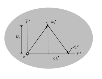
Figure 2: Path of light in the primed coordinate frame.

We consider two inertial frames of reference, $\bar{S}(\bar{x},\bar{y},\bar{z})$ and $\bar{S}^{\prime}(\bar{x}^{\prime},\bar{y}^{\prime},\bar{z}^{\prime})$, in a standard configuration. The origins of the reference frames are located inside an arbitrarily large isotropic homogeneous simple linear magneto-dielectric medium. The origins of the two systems coincide at time $t_{0}=0$ and all clocks are synchronized. At time $t_{c}=t_{c}^{\prime}=0$, a light pulse is emitted from the common origin along the positive $\bar{y}$ and $\bar{y}^{\prime}-$axes. In the $\bar{S}$ frame of reference, Fig. 1, the pulse is reflected by a mirror in the medium at $\bar{y}=D_{c}$ and returns to the origin at time $\Delta t_{c}=2D_{c}/c_{c}$, where $c_{c}$ is the speed of light in the medium. The trajectory of the light pulse in the $\bar{S}^{\prime}$ frame of reference is shown in Fig. 2. The translation of the $\bar{S}^{\prime}$ frame is transverse to the $\bar{y}$-axis so the distance from the mirror at $m_{c}^{\prime}$ to the $\bar{x}^{\prime}$-axis is $D_{c}$, the same as the distance from the mirror at $m_{c}$ to the $\bar{x}$-axis. Viewed from the $\bar{S}^{\prime}$ frame, the light pulse is emitted from the point $o$ at time $t_{c}^{\prime}=0$, is reflected from the mirror at point $m_{c}^{\prime}$, and is detected at the point $d_{c}^{\prime}$ at time $t_{c}^{\prime}=\Delta t_{c}^{\prime}$. During that time, the point of emission/detection has moved a distance $v_{c}\Delta t_{c}^{\prime}$.

By the Pythagorean theorem, we have

$$(c_{c}^{\prime}\Delta t_{c}^{\prime})^{2}=(c_{c}\Delta t_{c})^{2}+(v_{c}\Delta t_{c}^{\prime})^{2}\,,$$ (60)

where we have used reflection symmetry about the midpoint. We write the previous equation as [26]

$$\Delta t_{c}^{\prime}=\frac{\Delta t_{c}}{\sqrt{{c_{c}^{\prime}}^{2}/c_{c}^{2}-v_{c}^{2}/c_{c}^{2}}}$$ (61)

and define the ‘material’ Lorentz factor $\gamma_{c}$ by

$$\Delta t_{c}^{\prime}=\gamma_{c}\Delta t_{c}$$ (62)

such that

$$\gamma_{c}=\frac{1}{\sqrt{{c_{c}^{\prime}}^{2}/c_{c}^{2}-v_{c}^{2}/c_{c}^{2}}}\,.$$ (63)

In the Laue model, the speed of light in the dielectric depends on the velocity of the block in the Laboratory Frame of Reference. Here, the isotropy of an arbitrarily large homogeneous continuous dielectric medium at rest in the local frame of reference leads us to postulate that light travels at a uniform speed $c_{c}$ in the simple linear magneto-dielectric medium, basically the same reasoning that led to the Einstein postulate. Substituting

$$c_{c}^{\prime}=c_{c}$$ (64)

into Eq. (63), one obtains

$$\gamma_{c}=\frac{1}{\sqrt{1-v_{c}^{2}/c_{c}^{2}}}\,.$$ (65)

Using the definitions of the renormalized coordinates, we have $v_{c}=n_{m}v$ and $c_{c}=c/n_{e}$. Then,

$$\gamma_{c}=\frac{1}{\sqrt{1-n_{e}^{2}n_{m}^{2}v^{2}/c^{2}}}=\frac{1}{\sqrt{1-n^{2}v^{2}/c^{2}}}=\frac{1}{\sqrt{1-v^{2}/\bar{c}^{2}}}$$ (66)

for a simple linear magneto-dielectric medium ${\bar{c}}=c/n$. There is a different material Lorentz factor for each isotropic homogeneous simple linear magneto-dielectric medium. The vacuum Lorentz factor, Eq. (58), is a special case of Eq. (66) for $n_{e}=n_{m}=1$. The Rosen dielectric Lorentz factor, Eq. (59), is a special case of Eq. (66) for $n_{m}=1$.

VII Spacetime Setting

If a light pulse is emitted from the origin at a time $t=0$ into the empty vacuum of free space then spherical wavefronts are defined by

$$x^{2}+y^{2}+z^{2}=(x^{0})^{2}$$ (67)

in a flat, four-dimensional, vacuum Minkowski spacetime ${\sf S}_{M}(x^{0}=ct,x,y,z)$. Equation (67) underlies classical electrodynamics and its relationship to Einstein’s special relativity.

Consider a quasimonochromatic light pulse that is emitted from the origin $(\bar{x}=0,\bar{y}=0,\bar{z}=0)$ at ‘time’ $\bar{x}^{0}=0$ into an isotropic, homogeneous, simple linear magneto-dielectric medium, instead of the vacuum. In this medium, spherical wavefronts are defined by

$$\bar{x}^{2}+\bar{y}^{2}+\bar{z}^{2}=(\bar{x}^{0})^{2}$$ (68)

in an isotropic, homogeneous, flat, four-dimensional, non-Minkowski continuous material spacetime ${\sf S}_{c}(\bar{x}^{0},\bar{x},\bar{y},\bar{z})$. There will be a different material spacetime that is associated with each set of refractive indices, $n_{e}$ and $n_{m}$.

The four-dimensional ‘material’ light cone

$$\bar{x}^{2}+\bar{y}^{2}+\bar{z}^{2}-(\bar{x}^{0})^{2}=0$$ (69)

is embedded in the flat four-dimensional non-Minkowski ‘material’ spacetime ${\sf S}_{c}(\bar{x}^{0},\bar{x},\bar{y},\bar{z})$ that is associated with a linear, isotropic, homogeneous, simple linear magneto-dielectric medium. The basis functions, $\exp(-i(\bar{\omega}/c)(\bar{x}^{0}-{\bf\hat{k}}\cdot{\bf\bar{r}}))+c.c.$, where ${\bf\bar{r}}=(\bar{x},\bar{y},\bar{z})$, define the null surface, $\bar{x}^{0}={\bf\hat{k}}\cdot{\bf\bar{r}}$. Here, $\bar{\omega}$ can be associated with $n_{e}\omega$. Fig. 3 is a depiction of the intersection of the ‘material’ light cone with the $\bar{x}^{0}-\bar{x}$ plane in the flat material spacetime showing the null $\bar{x}^{0}=\bar{x}$. There will be a different material spacetime for each pair of material constants, $n_{e}$ and $n_{m}$, but the half-opening angle of the material light cone will always be $\alpha=\pi/4$ in that spacetime. The unit slope of the null in the $\bar{x}^{0}-\bar{x}$ plane of the non-Minkowski material spacetime is related to the coordinate speed of light in an isotropic, homogeneous, simple linear medium by

$$\frac{dx}{dt}=\frac{d\bar{x}}{d\bar{x}^{0}}\frac{d\bar{x}^{0}}{dt}\frac{dx}{d\bar{x}}=1\cdot\frac{c}{n_{e}}\cdot\frac{1}{n_{m}}=\frac{c}{n_{e}n_{m}}=\frac{c}{n}=\bar{c}\,.$$ (70)

This equation shows that the effective speed of light in a linear magneto-dielectric medium is attributable to two different effects: i) the renormalization of the timelike coordinate by $n_{e}^{-1}$ and ii) the renormalization of the spatial coordinates by $n_{m}$.

The usual characterization of events inside the vacuum light cone as timelike and events outside the vacuum light cone as spacelike also applies to the ‘material’ spacetime with events inside the renormalized ‘material’ light cone being timeline and events outside are spacelike. Čerenkov radiation, spontaneous emission, and mass-bearing particle dynamics in a simple linear medium will have to be treated carefully, if at all, because an atom or a charged particle must displace some of the linear medium that is effectively continuous at all length scales.

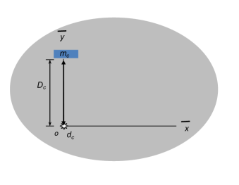
Figure 1: Path of light in the unprimed coordinate frame.

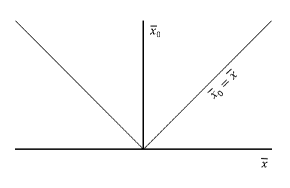
Figure 3: Null cone for light depicted in the $\bar{x}^{0}-\bar{x}$ plane of a flat, non-Minkowski material spacetime that corresponds to a linear magneto-dielectric medium.

VIII Lorentz transformation properties

Maxwellian continuum electrodynamics is based on averaging the interaction of microscopic fields with tiny bits of polarizable and magnetizable matter embedded in the vacuum. In the vacuum, Lorentz transformations of the coordinates follow from the invariance of

$$s^{2}=(x^{0})^{2}-x^{2}-y^{2}-z^{2}\,.$$ (71)

Then it makes sense to apply Lorentz invariance to the microscopic theory before the interactions are averaged in the continuum approximation and to apply Lorentz invariance to ‘real’ magneto-dielectric materials that are comprised almost entirely of empty space. Except, a macroscopic linear medium is defined as being continuous at all length scales from the very outset because the performing of such a macroscopic average from microscopic particles, fields, and interactions requires assumptions, approximations, and limiting behavior that become dubious in their complexity. Consequently, the assumption of Lorentz invariance for a macroscopic linear medium appears to be well-founded, based on the microscopic model, but it is manifestly not well-founded for macroscopic fields in continuous linear media.

By now, we should know that Lorentz invariance is not a symmetry of light in a macroscopic linear medium [29] and we cannot re-discretize or un-average the physics in order to impose Lorentz invariance. Instead, the invariance of

$$(\bar{s})^{2}=(\bar{x}^{0})^{2}-(\bar{x}^{1})^{2}-(\bar{x}^{2})^{2}-(\bar{x}^{3})^{2}$$ (72)

for monochromatic light in an arbitrarily large, isotropic, homogeneous simple linear medium imposes the conditions for linear medium-specific Lorentz-like transformations of the coordinates $(\bar{x}^{0},\bar{x}^{1},\bar{x}^{2},\bar{x}^{3})$ of a flat four-dimensional non-Minkowski material spacetime ${\sf S}_{c}(\bar{x}^{0},\bar{x},\bar{y},\bar{z})$. The special Lorentz-like transformations (with ${\bf v}$ parallel to the $\bar{x}$-axis) take the form

$$\bar{x}^{0^{\prime}}=\gamma_{c}\left(\bar{x}^{0}-(n_{e}n_{m}v/c)\bar{x}^{1}\right)=\gamma_{c}\left(\bar{x}^{0}-(nv/c)\bar{x}^{1}\right)$$ (73a)

$$\bar{x}^{1^{\prime}}=\gamma_{c}\left(\bar{x}^{1}-(n_{e}n_{m}v/c)\bar{x}^{0}\right)=\gamma_{c}\left(\bar{x}^{1}-(nv/c)\bar{x}^{0}\right)$$ (73b)

$$\bar{x}^{2^{\prime}}=\bar{x}^{2}$$ (73c)

$$\bar{x}^{3^{\prime}}=\bar{x}^{3}$$ (73d)

in a simple linear medium. The index-dependent Lorentz-like transformation confirms the observations of Ravndal [29] that the invariance properties of a linear medium differ from Lorentz invariance of the vacuum.

IX Tensor Formulation

With the advent of special relativity, the 3-vector formulation of electrodynamics became archaic. The tensor formalism allows the development of electrodynamics in the context of general properties of physical laws on Minkowski spacetime in a form that is manifestly invariant under Lorentz transformations. “Increasing the sophistication of the notation simplifies the appearance of the governing equations, revealing hidden symmetries and deeper meaning in the equations of electromagnetism” [48].

The fundamental laws of physics are formulated in the vacuum and Minkowski spacetime is empty. That is not considered to be a problem for continuous media because ‘real’ matter is mostly empty space. Except, Feynman’s [49] pedagogy makes it clear that there is a place in physics for macroscopic descriptions of fields and matter. Physical theory that is formulated for enumerated localized microscopic particles and microscopic fields interacting in a vacuum and defined on an empty Minkowski spacetime is always correct, but it is manifestly unjustified for macroscopic fields in an effective medium that is isotropic, homogeneous, and continuous at all length scales from the very outset.

In this section, we will develop an expressly macroscopic tensor formulation of continuum electrodynamics based on the macroscopic field equations, Eqs. (57d).

It is straightforward to use algebra and calculus in order to construct the energy–momentum tensor as a theorem of the macroscopic field equations. The derivation of the energy continuity equation follows the same procedure that was used to derive Poynting’s theorem, Eq. (9), as an identity of the Maxwell–Minkowski equations. We combine Eqs. (57d) to derive a theorem of macroscopic continuum electrodynamics in the form the scalar energy continuity equation

$$\frac{\partial{u_{c}}}{\partial\bar{x}^{0}}+\bar{\nabla}\cdot{\bf s}_{c}=0\,,$$ (74)

in the continuous material spacetime where

$$u_{c}=\frac{1}{2}({\bf\Pi}^{2}+{{\beta}\hskip-5.6pt{\beta}}^{2})$$ (75)

is the continuous energy density and

$${\bf s}_{c}=c{{\beta}\hskip-5.6pt{\beta}}\times{\bf\Pi}$$ (76)

is the continuous ‘material’ energy-flux vector. Similarly we combine Eqs. (57d) to form the vector momentum continuity theorem

$$\frac{\partial g^{i}_{c}}{\partial\bar{x}^{0}}+\sum_{j}\frac{\partial}{\partial\bar{x}^{j}}{{\sf W}_{c}}^{ij}=0$$ (77)

in component form, where

$${\bf g}_{c}=\frac{{{\beta}\hskip-5.6pt{\beta}}\times{\bf\Pi}}{c}$$ (78)

denotes the ‘material’ momentum density and

$${{\sf W}_{c}}^{ij}=-\Pi^{i}\Pi^{j}-\beta^{i}\beta^{j}+\frac{1}{2}({\bf\Pi}^{2}+{{\beta}\hskip-5.6pt{\beta}}^{2})\delta^{ij}$$ (79)

are the elements of a rank 3 matrix. Readers that are not familiar with the procedure used to derive Eq. (77) can consult Ref. [10], Sec. 6.8 of Ref. [35], or similar reference.

The scalar energy continuity equation, Eq. (74), and the scalar components of the vector momentum continuity equation, Eqs. (77), can be written, row-wise, as a single differential equation [42]

$$\bar{\partial}_{\beta}{\sf T}_{c}^{\alpha\beta}=0$$ (80)

as a matter of linear algebra, where

$$\bar{\partial}_{\beta}=\left(\frac{\partial}{\partial\bar{x}^{0}},\bar{\nabla}\right)$$ (81)

is the ‘material’ four-divergence operator. The ‘tensor’ differential equation, Eq. (80), is a theorem of the macroscopic field equations, Eqs. (57d), and the diagonally symmetric matrix ${\sf T}_{c}^{\alpha\beta}$ is

$${\sf T}_{c}^{\alpha\beta}\!=\!\left[\begin{matrix}{u}\!&{s}_{c}^{1}/c\!&{s}_{c}^{2}/c\!&{s}_{c}^{3}/c\cr c{g}_{c}^{1}&{\sf W}_{c}^{11}&{\sf W}_{c}^{12}&{\sf W}_{c}^{13}\cr c{g}_{c}^{2}&{\sf W}_{c}^{21}&{\sf W}_{c}^{22}&{\sf W}_{c}^{23}\cr c{g}_{c}^{3}&{\sf W}_{c}^{31}&{\sf W}_{c}^{32}&{\sf W}_{c}^{33}\cr\end{matrix}\right]\,,$$ (82)

by construction. Obviously, the intent is to identify ${\sf W}_{c}^{ij}$ as the continuum electrodynamic stress tensor, to identify ${\sf T}_{c}^{\alpha\beta}$ as the continuum electrodynamic energy–momentum tensor, and to identify the differential equation, Eq. (80), with the local electromagnetic conservation law.

We can re-formulate most of the other features of tensor electrodynamics, c.f., Sec. 11 of Ref. [35]. We construct the field strength tensor

$${\sf F}_{c}^{\alpha\beta}\!=\!\left[\begin{matrix}0\!&{\bf\Pi}_{x}\!&{\bf\Pi}_{y}\!&{\bf\Pi}_{z}\cr-{\bf\Pi}_{x}&0&-{{\beta}\hskip-5.6pt{\beta}}_{z}&{{\beta}\hskip-5.6pt{\beta}}_{y}\cr-{\bf\Pi}_{y}&{{\beta}\hskip-5.6pt{\beta}}_{z}&0&-{{\beta}\hskip-5.6pt{\beta}}_{x}\cr-{\bf\Pi}_{z}&-{{\beta}\hskip-5.6pt{\beta}}_{y}&{{\beta}\hskip-5.6pt{\beta}}_{x}&0\cr\end{matrix}\right]$$ (83)

and the dual field-strength tensor

$${\cal F}_{c}^{\alpha\beta}\!=\!\left[\begin{matrix}0\!&-{{\beta}\hskip-5.6pt{\beta}}_{x}\!&-{{\beta}\hskip-5.6pt{\beta}}_{y}\!&-{{\beta}\hskip-5.6pt{\beta}}_{z}\cr{{\beta}\hskip-5.6pt{\beta}}_{x}&0&-{\bf\Pi}_{z}&{\bf\Pi}_{y}\cr{{\beta}\hskip-5.6pt{\beta}}_{y}&{\bf\Pi}_{z}&0&-{\bf\Pi}_{x}\cr{{\beta}\hskip-5.6pt{\beta}}_{z}&-{\bf\Pi}_{y}&{\bf\Pi}_{x}&0\cr\end{matrix}\right]$$ (84)

such that

$$\bar{\partial}_{\alpha}{\sf F}_{c}^{\alpha\beta}=0$$ (85a)

$$\bar{\partial}_{\alpha}{\cal F}_{c}^{\alpha\beta}=0$$ (85b)

constitute an identity of the macroscopic field equations, Eqs. (57d). The energy–momentum tensor, Eq. (82),

$${\sf T}_{c}^{\alpha\beta}={\sf F}^{\alpha\mu}{\sf F}^{\beta}_{\hskip 2.8903pt\mu}+\frac{1}{4}g^{\alpha\beta}{\sf F}_{\mu\sigma}{\sf F}^{\mu\sigma}$$ (86)

and the Lagrangian density, Eq. (47),

$${\cal L}_{c}=\frac{1}{2}\left({\bf\Pi}^{2}-{{\beta}\hskip-5.6pt{\beta}}^{2}\right)=-\frac{1}{4}{\sf F}_{\alpha\beta}{\sf F}^{\alpha\beta}$$ (87)

are easily demonstrated by substitution of the field strength tensor, Eq. (83). Combining the definitions Eq. (78) and Eq. (76) we obtain

$${\bf s}=c^{2}{\bf g}\;.$$ (88)

The trace of the energy–momentum tensor vanishes

$$g_{\alpha\alpha}T_{c}^{\alpha\alpha}=0$$ (89)

corresponding to a continuous flow of massless particles. Substituting ${\bf s}=c^{2}{\bf g}$ into the energy–momentum tensor, Eq. (82), we have the symmetry property

$${\sf T}_{c}^{\alpha\beta}={\sf T}_{c}^{\beta\alpha}\,.$$ (90)

Using the symmetry property, Eq. (90), of the energy–momentum tensor, we obtain

$$\bar{\partial}_{\alpha}{\sf T}_{c}^{\alpha\beta}=0$$ (91)

from Eq. (80).

Returning to Maxwellian continuum electrodynamics for a moment, the well-known Minkowski energy–momentum tensor can be constructed by linear algebra from macroscopic energy and momentum continuity equations that are theorems of the Maxwell–Minkowski equations, but the Minkowski energy–momentum tensor is not symmetric. The Faraday law, Eq. (3b), in a linear medium

$$\nabla\times{\bf E}-\frac{\partial{\bf B}}{\partial(ct)}=0$$ (92)

has the same timelike coordinate as the Faraday law in the vacuum Minkowski spacetime, $S_{v}(x^{0}=ct,z,y,z)$. In contrast, the Maxwell–Ampère law, Eq. (3a),

$$\nabla\times{\bf B}+\frac{\partial{\bf E}}{\partial(ct/n^{2})}=0$$ (93)

has a renormalized temporal coordinate that we would associate with the non-Minkowski spacetime, $S_{?}(ct/n^{2},z,y,z)$. These equations cannot be combined self-consistently to form valid energy and momentum continuity equations because they are based on different coordinate systems and belong in different spacetimes. The Minkowski energy-momentum tensor is not symmetric because the macroscopic Maxwell–Minkowski equations are inconsistently defined in a pathological spacetime. In contrast, all of the new macroscopic field equations are in the continuous ‘material’ spacetime, ${\sf S}_{c}(\bar{x}^{0},\bar{x},\bar{y},\bar{z})$ that is consistent with the electric and magnetic properties of the linear medium.

X Experimental Confirmation

X.1 The Balazs thought experiment

In 1953, Balazs [33] proposed a thought experiment to resolve the Abraham–Minkowski controversy. The thought experiment was based on the law of conservation of momentum and a theorem that the center of mass-energy moves at a uniform velocity [50]. The application of this theorem indicates that microscopic constituents of the material that carry mass also travel with the field.

The relativistic total energy

$$E=\left({\bf p}\cdot{\bf p}c^{2}+m^{2}c^{4}\right)^{1/2}$$ (94)

becomes the Einstein formula $E=mc^{2}$ for massive particles in the limit ${\bf v}/c\rightarrow 0$. For massless particles, like photons, Eq. (94) becomes

$${\bf p}=\frac{E}{c}{\bf\hat{e}}_{k}=\frac{\hbar\omega_{0}}{c}{\bf\hat{e}}_{k}\,,$$ (95)

where ${\bf\hat{e}}_{k}$ is a unit vector in the direction of motion. Equation (95) defines the instantaneous momentum of a photon traveling at speed $c$.

Consider a photon that enters a material that is composed of electric and magnetic dipoles embedded in the vacuum. The photon travels at speed $c$ between scattering events [49], but due to scattering the effective speed of the photon in the incident direction is $c/n$. Due to the reduced effective speed of individual photons, an unimpeded, inviscid, incoherent, incompressible flow of non-interacting photons in the continuum limit travels at an average speed of $c/n$ and the longitudinal extent of the field in the direction of the flow is reduced by a factor of $n$. Then the photon density, the energy density, and the momentum density are increased by a factor $n$. Integrating the quantities over the reduced longitudinal width of the field, the energy and momentum are constant as the field leaves vacuum and enters a dielectric medium without needing to assume any material motion. Due to the decreased velocity and increased density, the energy velocity of the ensemble is $c=n\cdot c/n$. Then the energy velocity of a field into and through a linear medium moves at a constant speed $c$ because of the enhanced photon density. The mass-polariton (MP) model [51] of propagation of the electromagnetic field in which the propagating field combines with mass-bearing particles of a continuous dielectric is not supported. Because the density of photons is larger due to the reduced average velocity, the higher density of photons corresponds to an increase in energy density and momentum density in the macroscopic field. Then, the macroscopic field in a linear medium that corresponds to the energy of a single photon occupies a smaller volume than the volume occupied in the vacuum. Likewise, a smaller volume of the field is associated with the momentum of a single photon. An additional issue with the photon description of light propagation in a continuous dielectric is illustrated by the commingling of macroscopic fields and the macroscopic refractive index with microscopic photon momentum and momentum states in a description of photon recoil momentum in a medium [52].

As an electromagnetic field propagates from vacuum into a simple linear medium, the ‘effective’ velocities of photons in the field are reduced creating an enhancement of the classical energy density $u_{c}=({\bf\Pi}^{2}+{{\beta}\hskip-5.6pt{\beta}}^{2})/2$ and the classical momentum density ${\bf g}_{c}={{\beta}\hskip-5.6pt{\beta}}\times{\bf\Pi}/c$, compared to the vacuum. For finite pulses in a dielectric, the enhanced energy density is offset by a narrowing of the pulse so that the electromagnetic energy

$$U_{total}=\int_{\Sigma}\frac{1}{2}\frac{{\bf\Pi}^{2}+{{\beta}\hskip-5.6pt{\beta}}^{2}}{c}dv\,,$$ (96)

is time independent for quasimonochromatic fields in the plane-wave limit. The electromagnetic energy is the total energy by virtue of being constant in time. Likewise, the electromagnetic momentum,

$${\bf G}_{total}=\int_{\Sigma}\frac{{{\beta}\hskip-5.6pt{\beta}}\times{\bf\Pi}}{c}dv\,,$$ (97)

is time independent and is the total momentum.

Invoking the Einstein mass–energy equivalence, it is argued that some microscopic constituents of the dielectric must be accelerated and then decelerated by the field; otherwise the theorem that the center of mass–energy moves at a constant velocity is violated [14]. For a distribution of particles of mass $m_{i}$ and velocity ${\bf v}_{i}$, the total momentum

$${\bf P}_{total}=\sum_{i}m_{i}{\bf v}_{i}$$ (98)

is the sum of the momentums of all the particles $i$ in the distribution. If the mass of each particle $m_{i}$ is constant, the statement that the velocity of the center of mass

$${\bf v}_{CM}=\frac{\sum_{i}m_{i}{\bf v}_{i}}{\sum_{i}m_{i}}$$ (99)

is constant is a statement of conservation of total momentum.

Because of the enhanced momentum density of the field in a dielectric, the differential of electromagnetic momentum

$$\delta{\bf p}=\frac{{{\beta}\hskip-5.6pt{\beta}}\times{\bf\Pi}}{c}\delta v$$ (100)

that is contained in an element of volume $\delta v$ (a ‘particle’), is a factor of $n$ greater than in the vacuum. Then the mass–energy of each ‘particle’ $m_{i}$ is not constant as would be required for the center-of-mass theorem. For a finite pulse, the narrower pulse width offsets the enhanced momentum density allowing the macroscopic electromagnetic momentum, like the macroscopic electromagnetic energy, to be constant in time as the field enters, and exits, the simple linear medium through the gradient-index antireflection coating. Consequently, there is no need to hypothesize mass-polariton quasiparticles [51] or any other material constituents of the continuous linear medium to be in motion in order to preserve the conservation of linear momentum. Even though the velocity of light slows to $c/n$, the hypothetical Minkowski pull-force is also disproved.

X.2 The Jones–Richards experiment

One of the enduring questions of the Abraham–Minkowski controversy is why the Minkowski momentum is so often measured experimentally while the Abraham form of momentum is so favored in theoretical work. We now have the tools to answer that question. The Minkowski momentum is not measured directly, but inferred from a measured index dependence of the optical force on a mirror placed in a dielectric fluid [1, 15, 34]. The force on the mirror is

$${\bf F}=\frac{d}{d\bar{x}_{0}}(2c{\bf G}_{total})=\frac{d}{d\bar{x}_{0}}\int_{V}2{{\beta}\hskip-5.6pt{\beta}}\times{\bf\Pi}\,\delta(z)dv\,,$$ (101)

which depends on the total momentum density, Eq. (97). If we were to assume ${\bf F}=2d{\bf G}_{M}/dt$, which is the relation between momentum and force in an otherwise empty Minkowski spacetime, then we would write

$${\bf F}=\frac{1}{c}\frac{d}{dt}\int_{V}{2{\bf D}\times{\bf B}}\,\delta(z)dv\,.$$ (102)

Then one might use Eq. (102) of interpret the results of an experiment in such a way that the momentum density of the field in the dielectric fluid is the Minkowski momentum density.

The measured force on the mirror in the Jones–Richards experiment [34] is consistent with both Eqs. (101) and Eqs. (102), depending on what theory you use to interpret the results. Clearly an experiment that measures force, instead of directly measuring the change in momentum in the dielectric, will not conclusively distinguish the momentum density. Specifically, the Jones–Richards experiment does not prove that the Minkowski momentum density is the momentum density in the dielectric, as has been argued, nor does it prove that the continuum momentum density, Eq. (78), is the momentum density in the dielectric.

XI Summary

It has been said that physics is an experimental science and that physical theory must be constructed on the solid basis of observations and measurements. That is certainly true for serendipitous discoveries like x-rays and radioactivity; But Maxwell [53] used inductive reasoning to modify the Ampère law and construct the laws of electrodynamics two decades before Hertz [54] demonstrated the existence of electromagnetic waves. Later, Einstein’s theory of relativity was criticized for violating the ‘well-established’ principle of absolute simultaneity [47]. The law of conservation of mass became the law of conservation of mass–energy long before any measurements of relativistic mass effects. Mathematics is the language of physics and there are many other examples (nonlinear optics, high-energy physics, negative refraction, etc.) in which theoretical physics leads experiments by a substantial period of time.

Axiomatic formal theory is a cornerstone of abstract mathematics. The contradiction of valid theorems of Maxwellian continuum electrodynamics proves, unambiguously, that Maxwellian continuum electrodynamics is false. Having proven Maxwellian continuum electrodynamics to be manifestly false, as it has been proven false by the Abraham–Minkowski momentum contradiction for over a century, we established a reformulation of theoretical continuum electrodynamics by deriving equations of motion for the macroscopic fields from a generalized Lagrangian field theory. For every simple linear medium there is a different set of equations of motion based in a different continuous ‘material’ spacetime with coordinates that are renormalized by the linear permittivity and linear permeability. The Abraham–Minkowski controversy is trivially resolved because the tensor total energy–momentum continuity theorem, the total energy–momentum tensor, the total momentum, and the total energy are fully electromagnetic, unique, and conserved for a closed (complete) model system consisting of a simple linear dielectric block draped with a gradient-index antireflection coating that is illuminated by quasimonochromatic light.

References

- [1] R. N. C. Pfeifer, T. A. Nieminen, N. R. Heckenberg, and H. Rubinsztein-Dunlop, Colloquium: momentum of an electromagnetic wave in dielectric media, Rev. Mod. Phys. 79, 1197–1216 (2007).
- [2] I. Brevik, Radiation Forces and the Abraham–Minkowski Problem, Mod. Phys. Lett. A 33, 1830006 (2018).
- [3] I. Brevik, Minkowski momentum resulting from a vacuum-medium mapping procedure, and a brief review of Minkowski momentum experiments, Ann. Phys. (N Y) 377, 10-21 (2017).
- [4] I. Brevik, Analysis of recent interpretations of the Abraham–Minkowski problem, Phys. Rev. A 98, 043847 (2018).
- [5] C. Wang, Can the Abraham Light Momentum and Energy in a Medium Constitute a Lorentz Four-Vector, J. Mod. Phys. 4, 1123-1132 (2013).
- [6] J. P. Gordon, Radiation forces and momenta in dielectric media, Phys. Rev. A 8, 14–21 (1973).
- [7] P. L. Saldanha and J. S. O. Filho, Hidden momentum and the Abraham–Minkowski debate, Phys. Rev. A 95, 043804 (2017).
- [8] V. P. Torchigin and A. V. Torchigin, Resolution of the Age-Old Dilemma about a Magnitude of the Momentum of Light in Matter, Phys. Res. Int. 2014, 12636.
- [9] D. J. Griffiths, Resource Letter EM-1: Electromagnetic Momentum, Am. J. Phys. 80, 7–18 (2012).
- [10] P. W. Milonni and R. W. Boyd, Momentum of light in a dielectric medium, Adv. Opt. Photonics 2, 519–553 (2010).
- [11] B. A. Kemp, Resolution of the Abraham–Minkowski debate: Implications for the electromagnetic wave theory of light in matter, J. Appl. Phys. 109, 111101 (2011).
- [12] B. A. Kemp, Macroscopic Theory of Optical Momentum, Prog. Opt. 20, 437–488 (2015).
- [13] P. Penfield, Jr. and H. A. Haus, Electrodynamics of Moving Media, MIT Press, Cambridge (1967).
- [14] S. M. Barnett, Resolution of the Abraham–Minkowski dilemma, Phys. Rev. Lett. 104, 070401 (2010).
- [15] S. M. Barnett and R. Loudon, The enigma of optical momentum in a medium, Phil. Trans. A 368, 927–939 (2010).
- [16] M. Kranys, The Minkowski and Abraham Tensors, and the Non-Uniqueness of Non-Closed Systems, Int. J. Engng. Sci. 20, 1193-1213 (1982).
- [17] T. Ramos, G. F. Rubilar and Y. N. Obukhov, Relativistic analysis of the dielectric Einstein box: Abraham, Minkowski, and the total energy–momentum tensors, Phys. Lett. A 375, 1703–1709 (2011).
- [18] H. Minkowski, Die Grundgleichungen für die elektromagnetischen Vorgänge in bewegten Körpern, Natches. Ges. Wiss. Göttingen, 53-111 (1908).
- [19] M. Abraham, Zur Elektrodynamik bewegter Körper, Rend. Circ. Mat. Palermo, 28, 1-28 (1909).
- [20] I. Brevik, Experiments in phenomenological electrodynamics and the electromagnetic energy–momentum tensor, Phys. Rep. 52, 133-201 (1979).
- [21] M. E. Crenshaw, Electromagnetic momentum and the energy-momentum tensor in a linear medium with magnetic and dielectric properties, J. Math. Phys. 55, 042901 (2014).
- [22] D. Giulini, The Rich Structure of Minkowski Space in: V. Petkov (ed.), Minkowski Spacetime: A Hundred Years Later, Fundamental Theories of Physics, 165, 83-132, Springer Verlag, Dordrecht, 2010.
- [23] R. W. Fox and A. T. McDonald, Introduction to Fluid Mechanics, Chap. 5 (Wiley, New York 1978).
- [24] H. Goldstein, Classical Mechanics, Chap. 12 (Addison-Wesley, Reading, 1980).
- [25] C. Cohen-Tannoudji, J. Dupont-Roc, and T. Grynberg, Photons and Atoms (Wiley, New York 1989).
- [26] M. E. Crenshaw, Reconciliation of the Rosen and Laue theories of special relativity in a linear dielectric medium, Am. J. Phys. 87, 296–300 (2019).
- [27] M. Laue, Die Mitfürung des Lichtes durch bewegte Körper nach dem Relativitatspriinzip, Ann. Phys. (Berlin) 328, 989–990 (1907).
- [28] N. Rosen Special theories of relativity, Am. J. Phys 20, 161–164 (1952).
- [29] F. Ravndal, Effective electromagnetic theory for dielectric media, http://arxiv.org/pdf/0804.4013v3.pdf (2008).
- [30] D. Giulini Laue’s Theorem Revisited: Energy–Momentum Tensors, Symmetries, and the Habitat of Globally Conserved Quantities, Int. J. Geom. Methods Mod. Phys. 15, 1850182 (2018).
- [31] C. Wang, von Laue’s theorem and its applications, Can. J. Phys. 93, 1470-1476 (2015).
- [32] D. E. Neuenschwander, Emmy Noether’s Wonderful Theorem, (John Hopkins University Press, Baltimore, 2011).
- [33] N. L. Balazs, The energy–momentum tensor of the electromagnetic field inside matter, Phys. Rev. 91, 408–411 (1953).
- [34] R. V. Jones and J. C. S. Richards, The Pressure of Radiation on a Refracting Medium, Proc. R. Soc. London, Ser. A 221, 480–498 (1954).
- [35] J. D. Jackson, Classical Electrodynamics (John Wiley, 1975).
- [36] D. J. Griffiths, Introduction to Electrodynamics, (Prentice Hall, New Jersey, 1981).
- [37] A. Zangwill, Modern Electrodynamics (Cambridge Univ. Press, 2011).
- [38] W. Rindler, Introduction to Special Relativity (Oxford University Press, New York, 1982).
- [39] M. Mansuripur, Electromagnetic force and torque in ponderable media, Opt. Express 16, 14821–14835 (2008).
- [40] M. Masuripur and A. R. Zakharian, Maxwell’s macroscopic equations, the energy–momentum postulates, and the Lorentz law of force, Phys. Rev. E /textbf 79, 026608 (2009).
- [41] J. B. Marion and M. A. Heald, Classical Electromagnetic Radiation, 2nd. ed., (Academic Press, Orlando, 1980)
- [42] M. E. Crenshaw and T. B. Bahder, Energy–momentum tensor for the electromagnetic field in a dielectric, Opt. Commun. 284, 2460–2465 (2011).
- [43] M. E. Crenshaw, Alternative formulation of the macroscopic field equations in a linear magneto-dielectric medium: Field equations, OSA Continuum 3, 246–252 (2020).
- [44] G. L. Nabor, The Geometry of Minkowski Spacetime, p. 1 (Dover, New York, 2003).
- [45] M. Born and E. Wolf, Principles of Optics, Sec. 2.3.1 (Pergamon Press, Oxford, 1989).
- [46] M. E. Crenshaw, Representation Independent Boundary Conditions for a Piecewise-Homogeneous Linear Magneto-dielectric Medium, AIP Advances 9, 075102 (2019).
- [47] P. Ehrenfest (1927) cited in N. Bohr, Collected Works, Volume 6 - Foundation of Quantum Physics I (1926-1932), p. 416, ed. by J. Kalckar, (North-Holland, Amsterdam, 1985).
- [48] K. F. Warnick and P. Russer Differential Forms and Electromagnetic Field Theory, Prog. Electromagn. Res. 148, 83–112 (2014).
- [49] R. P. Feynman, R. B. Leighton, and M. L. Sands, The Feynman Lectures on Physics, Vol. 1, Sec. 31 (Addison–Wesley, Reading, 1963).
- [50] T. H. Boyer, Illustrations of the Relativistic Conservation Law for the Center of Energy, Am. J. Phys. 73, 953–961 (2005).
- [51] M. Partanen, T. Hayrynen, J. Oksanen, and J. Tulkki, Photon mass drag and the momentum of light in a medium, Phys. Rev. A 95, 063850 (2017).
- [52] G. K. Campbell, A. E. Leanhardt, J. Mun, M. Boyd, E. W. Streed, W. Ketterle, and D. E. Pritchard, Photon Recoil Momentum in Dispersive Media, Phys. Rev. Lett. 94, 170403 (2005).
- [53] J. C. Maxwell, Phil. Trans. Roy. Soc. Lon., 155, 459–512 (1865).
- [54] H. R. Hertz, Ueber die Einwirkung einer geradinigen electrischen Schwingung auf eine benachbarte Strombahn, Ann. Phys. (Berlin), 270, 155-170 (1888).