Static and dynamic scaling behavior of a polymer melt model with triple-well bending potential
Abstract
We perform molecular-dynamics simulations for polymer melts of a coarse-grained polyvinyl alcohol model that crystallizes upon slow cooling. To establish the properties of its high temperature liquid state as a reference point, we characterize in detail the structural features of equilibrated polymer melts with chain lengths at a temperature slightly above their crystallization temperature. We find that the conformations of sufficiently long polymers with obey essentially the Flory’s ideality hypothesis. The chain length dependence of the end-to-end distance and the gyration radius follow the scaling predictions of ideal chains and the probability distributions of the end-to-end distance, and form factors are in good agreement with those of ideal chains. The intrachain correlations reveal evidences for incomplete screening of self-interactions. However, the observed deviations are small. Our results rule out any pre-ordering or mesophase structure formation that are proposed as precursors of polymer crystallization in the melt. Moreover, we characterize in detail primitive paths of long entangled polymer melts and we examine scaling predictions of Rouse and the reptation theory for the mean squared displacement of monomers and polymers center of mass.
Introduction
Polymer melts are dense liquids consisting merely of macromolecular chains. The main characteristic of polymer melts is their high-packing density which leads to overlapping of pervaded volume of their chains Rubinstein and Colby (2003). As a result, density fluctuations in a melt are small and similar to a simple fluid every monomer is isotropically surrounded by other monomers that can be part of the same chain or belong to other chains. As a consequence the chains conformations in the molten state are close to random walks. Nevertheless, the crystallization of polymer melts remarkably differs from monomeric liquids due to chain connectivity constraints that must be compatible with lattice spacings of a crystalline structure. Upon cooling of a crystallizable polymer melt, a semicrystalline structure emerges that comprises of regularly packed, extended chain sections surrounded by amorphous strands Mandelkern (1990).
Despite intensive research, the mechanism of polymer crystallization is still poorly understood as this process is determined by an intricate interplay of kinetic effects and thermodynamic driving force Keller (1968); edited by J.-U. Sommer and Reiter (2003). From theoretical perspective, attempts have been made to understand thermodynamics of polymer crystallization. These efforts include lattice-based model Flory (1956), Landau-de Gennes types of approach Olmsted et al. (1998) and density functional theory Sushko et al. (2001); McCoy et al. (1991). Among these, the density-functional theory is a particularly promising approach as it can predict equilibrium features of inhomogeneous semicrystalline structure from the homogeneous melt structure provided that a suitable free-energy functional is employed and accurate information about chain conformations and structure of polymeric liquids is supplied Oxtoby (2002). Such an input can be obtained from simulations of a crystallizable polymer melt that allow us to compute the intrachain and interchain correlation functions. Here, our aim is to characterize conformations of a crystallizable polymer melt model known as coarse-grained polyvinyl alcohol (CG-PVA) Meyer and Müller-Plathe (2001). Owing to its coarse-grained nature, this model allows for simulations of large-scale structure of semicrystalline polymers.
The CG-PVA is a bead-spring polymer model that is obtained by a systematic coarse-graining from atomistic simulations of polyvinyl alcohol Reith et al. (2001). The coarse-graining procedure maps all the atoms of a monomer into one bead and a bending potential is extracted from the bond-angle distribution of atomistic simulations of PVA polymers. The main distinctive feature of the model is its triple-well intrachain bending rigidity that leads to formation of chain-folded crystallites upon slow cooling of the melt Meyer and Müller-Plathe (2001); Jabbari-Farouji et al. (2015a). Although the model does not take into account the intermolecular hydrogen bonding interactions, it reproduces the main features of polymer crystallization such as lamella formation. Recently, the CG-PVA model has been employed to study the dependence of polymer crystallization on the chain length Jabbari-Farouji et al. (2017); Triandafilidi et al. (2016). To understand the influence of chain length and entanglements on the melt crystallization Luo and Sommer (2013, 2016), the properties of its high-temperature liquid state need to be firmly established as a reference point. Here, we focus on the static and dynamic properties of CG-PVA polymer melts at a temperature which is 1.1 times the crystallization temperature.
The prior studies of structural properties of this system have been limited to static properties of short chains Vettorel et al. (2007) with purely repulsive interactions. Here, we present the results for CG-PVA polymer melts with with attractive interactions. Characterizing the conformational features of longer polymer melts, we accurately determine the persistence length, the Flory’s characteristic ratio and the entanglement length of CG-PVA polymers. Examining carefully the consequences of the triple-well bending potential on chain conformations, we barely find any evidence of pre-ordering or microstructure formation as precursors of crystallization. Encompassing a crossover from short unentangled chains to the entangled ones, we examine the credibility of Flory’s ideality hypothesis and manifestations of incomplete screening of excluded volume and hydrodynamic interactions on the structural and dynamical features of entangled polymer melts with a finite persistence length.
Flory’s ideality hypothesis states that polymer conformations in a melt behave statistically as ideal random-walks on length scales much larger than the monomer’s diameter Flory (1969); Doi and Edwards (1986). This ideality hypothesis is a mean-field result that relies on the negligibility of density fluctuations in polymer melts. Therefore, its validity is not taken for granted. Indeed, the computational studies of fully flexible long polymers for both lattice (bond fluctuation) and continuum (bead-spring) models have revealed noticeable deviations from the ideal chain behavior Wittmer et al. (2004, 2007a, 2007b); Beckrich et al. (2007); Hsu (2014). The theoretical calculations show that these deviations result from the interplay between the chain connectivity and the melt incompressibility which foster an incomplete screening of excluded volume interactions Wittmer et al. (2007a); Beckrich et al. (2007); Semenov (2010). However, a recent study of conformational properties of long locally semiflexible polymer melts demonstrates that the deviations diminish as the chains bending stiffness increases and the conformations of sufficiently stiff chains are well described by the theoretical predictions for ideal chains Hsu and Kremer (2016).
Investigation of the static scaling behavior of locally semiflexible CG-PVA polymer melts confirms that CG-PVA polymers display globally random-walk like conformations. Notably, for chains with , the results of the end-to-end distance, gyration radius, the probability distribution functions and the chain structure factor are in good agreement with the theoretical predictions for ideal chains. However, inspection of intrachain correlations reveals some evidences for deviations from ideality. The mean-square internal distances of long chains are slightly swollen compared to ideal chains due to incomplete screening of excluded volume interactions. Additionally, the second Legendre polynomial of angle between bond vectors exhibits a power law decay for curvilinear distances larger than the persistence length providing another testimony for self-interaction of chains. Nonetheless, we note that these visible deviations are small.
The remainder of the paper is organized as follows. In Sec. II, we briefly review the CG-PVA model and provide the simulation details. We present a detailed analysis of conformational and structural features of polymer melts in Sec. III and we compare simulation results to the theoretical predictions for ideal chains. We investigate conformational properties of the primitive paths of long chains in section IV where we determine the entanglement length of fully equilibrated CG-PVA chains. Sec. V explores the segmental motion of polymers at different characteristic timescales and examines the scaling laws predicted by the Rouse model and the reptation theory Rubinstein and Colby (2003); de Gennes (1979); Doi and Edwards (1986). Finally, we summarize our main findings and discuss our future directions in section VI.
Model and simulation details
We equilibrate polymer melt configurations of the coarse-grained polyvinyl alcohol (CG-PVA) model using molecular dynamics simulations. In the following, we first briefly review CG-PVA model and then provide the details of simulations.
Recap of the CG-PVA model
In the CG-PVA bead-spring model, each bead of the coarse-grained chain with diameter nm corresponds to a monomer of the PVA polymer. The fluctuations of the bond length about its average value are restricted by a harmonic potential with a bond stiffness constant
| (1) |
that leads to bond length fluctuations with a size much smaller than the monomer diameter. Monomers of distinct chains and the same chain that are three bonds or farther apart interact by a soft 6-9 Lennard-Jones potential,
| (2) |
in which and . Here, K is the reference temperature of the PVA melt Meyer and Müller-Plathe (2001). We truncate and shift the Lennard-Jones potential at in our simulations. Our choice of is different from initial studies where the non-bonded interactions were truncated at the minimum of the LJ potential and thus were purely repulsive. The purely repulsive model was initially used to study structure formation in the quiescent state Meyer and Müller-Plathe (2001, 2002); Luo and Sommer (2013, 2016). The attractive part is needed for non-equilibrium studies of deformation Jabbari-Farouji et al. (2015a, b, 2017). Note that the choice of leads to an increase of density by about 10 % with respect to the purely repulsive conditions. However, the structural properties of the melt remain essentially unaffected.
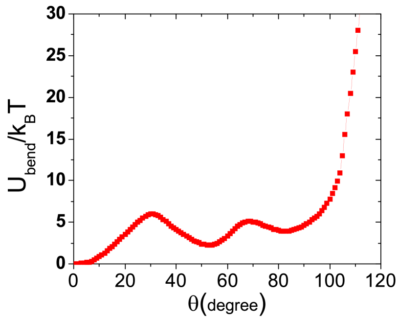
The distinguishing characteristic of the CG-PVA model is its triple-well angle-bending potential Meyer and Müller-Plathe (2001) as presented in Fig. 1. This bond angle potential is determined directly from atomistic simulations by Boltzmann inversion of the probability distribution of the bond angle Reith et al. (2001); Meyer and Müller-Plathe (2001). The minima of reflect the specific states of two successive torsion angles at the atomistic level and they correspond to three energetically favorable states, trans-trans, trans-gauche and gauche-gauche. Therefore, the bending potential retains semiflexibility of chains originated from the torsional states of the atomistic backbone Meyer and Müller-Plathe (2001).
Units and simulation aspects
| 2.06 | 0.615 | 1.63 | |||
| 2.20 | 1.08 | 2.98 | |||
| 2.28 | 1.79 | 4.79 | |||
| 2.30 | 2.35 | 6.09 | |||
| 2.33 | 3.17 | 8.11 | |||
| 2.34 | 4.69 | 11.73 | |||
| 2.35 | 6.68 | 16.53 | |||
| 8.25 | 20.31 | ||||
| 2.35 | 10.85 | 26.49 | |||
| 2.36 | 15.11 | 37.27 |
We carry out molecular dynamics simulations of CG-PVA polymers with chains lengths using LAMMPS Plimpton (1995). We report the distances in length unit nm. Meyer and Müller-Plathe (2001). The time unit from the conversion relation of units is with the monomer mass . The starting melt configurations are prepared by generating an ensemble of (number of chains) self-avoiding random walks composed of monomers with an initial density of . To remove the interchain monomer overlaps, we use a slow push off method in which initially a very weak LJ potential with and a very small is switched on. Next, the range and strength of Lennard-Jones potential are gradually increased to their final values. We equilibrate disordered melt structures in the NPT ensemble using a Berendsen barostat and a Langevin thermostat with friction constant . The temperatures and pressures are reported in reduced units and , equivalent to K and bar in atomistic simulations. The time step used through all the simulations is . The chosen melt temperature is about 10% higher than the crystallization temperature of long polymer melts () obtained at a cooling-rate of Jabbari-Farouji et al. (2017).
The polymer configurations for were equilibrated until the average monomers mean-square displacement is equal or larger than their mean square end-to-end distance . The time for which is a measure of the relaxation time and it is comparable to the Rouse time for the short chains and the disengagement time for the entangled chains Doi and Edwards (1986) as will be verified in section V. Polymer melts with , were equilibrated until is comparable to their mean-square gyration radius . Table 1 provides a summary of configurations of polymers and the simulation time for equilibration after push off stage in units of . Then, the data for characterization of static and dynamic properties are acquired.
In order to analyze the static properties of CG-PVA polymers, we extract from the polymer configurations the normalized probability distribution functions of the internal distances, the gyration radius, the bond length and angle of polymers as well as the bond length and angle of their primitive paths. We acquire the numerical probability distribution of a desired observable by accumulating a histogram of a fixed width . Then, we calculate the normalized probability distribution function as .
Structural features of CG-PVA polymer melts
We first present the results on the chain-length dependence of the mean square end-to-end distance and the gyration radius for chain sizes in the range . The mean square end-to-end distance is defined as
| (3) |
and the mean square gyration radius is given by
| (4) |
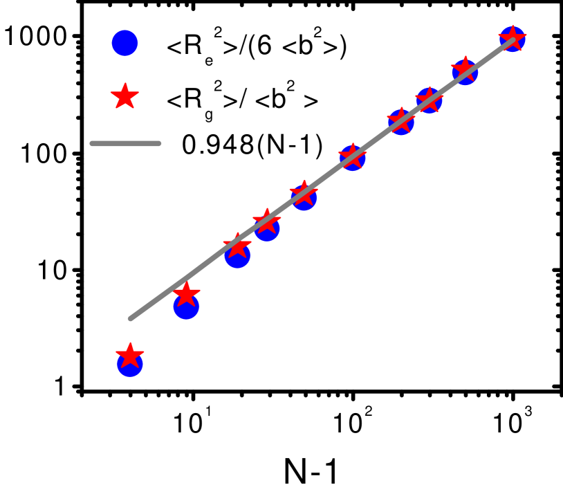
where is the position of th monomer of chain number and is the center of mass position of the th polymer chain in a sample. Here, includes an averaging over equilibrated configurations that are apart for the shorter chains and apart for the longer chains with . Fig. 2 shows and as a function of chain length . Here, denotes the mean-square bond length that is independent of the chain length. The longer chains with follow the relation valid for ideal chains de Gennes (1979). For shorter chains the ratio is in the range . Additionally, chains with follow the scaling behavior of ideal chains . The extracted scaling exponent from fitting versus with a power law gives that is identical to the value for the ideal chains. The observed scaling behavior for the mean square end-to-end distance and the gyration radius of CG-PVA polymers with suggests that long polymers behave like ideal chains. In the following, we investigate in more detail the conformational statistics of individual chains, and compare them to the theoretical predictions for ideal chains de Gennes (1979); Rubinstein and Colby (2003) .
Intrachain correlations

We begin by characterizing the intrachain correlations for both monomer positions and bond orientations. To quantify the positional intrachain correlations, we calculate the mean-square internal distances (MSID) for various chain lengths defined as
| (5) |
where is the curvilinear (chemical) distance between the th monomer and the th monomer along the same chain. MSID is a measure of internal chain conformation that can be used to evaluate the equilibration degree of long polymers.
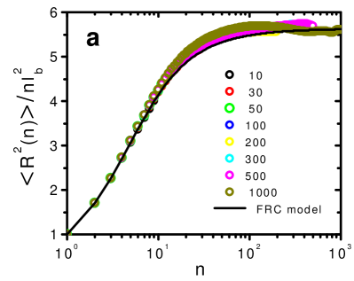
In Fig. 3a, we present the rescaled mean square internal distance, obtained by averaging over polymer melt configurations that are ( ) apart for short (long) chains. Up to , we find a good collapse of all the MSIDs. However, for larger curvilinear distances, the MSIDS of longer chains are slightly larger but all follow the same master curves suggesting that longer chains are a bit swollen due to chains self-interactions. Note that the deviations of of chains for curvilinear distances from other long chains are due to their poor equilibration. These results show that the chains are equilibrated at shorter length scales but their large-scale conformation still needs much longer equilibration time where is the entanglement length as will be discussed in the section IV.
From the asymptotic behavior of mean square end-to-end distances of long CG-PVA chains, we can extract their characteristic ratio and Kuhn length . The characteristic ratio is defined by the relation where is the average bond length. From MSID of longer polymers, and , we obtain . The Kuhn length gives us the effective bond length of an equivalent freely jointed chain which has the same mean square end-to-end distance and the same maximum end-to-end to distance Rubinstein and Colby (2003). For a freely jointed chain with Kuhn segments with bond length , we have and . For CG-PVA polymers, we find and . Equating and of the CG-PVA chains with those of the equivalent freely jointed chain, we obtain .
Next, we compare the mean square internal distance of CG-PVA polymers with of the generalized freely rotating chain (FRC) model Flory (1969); Honnell et al. (1990a) for ideal chains. If the excluded volume interactions between different parts of a certain polymer are screened, one expects the FRC model to provide a good description of CG-PVA polymer melts. of FRC model only depends on the value of where is the angle between any two successive bonds in a chain. It is given by
| (6) |
The value of for the CG-PVA model can be obtained from as
| (7) |
where is presented in Fig. 1. Doing the integration in Eq. (6) at numerically, we obtain . We can also directly infer from the MD simulations results as where is the th unit bond vector of the th chain and the averaging is carried out over all the chains and 100-500 equilibrated polymer melt configurations that are apart. From MD simulations, we deduce the universal value of independent of the chain length. This value agrees well with the Boltzmann-averaged mean value.
In Fig. 3a, we have also included the MSID of an equivalent freely rotating chain with . We find that MSIDs of short chains fully agree with that of the freely rotating chain model whereas the MSIDs of longer chains present noticeable deviations from the FRC theory for . Hence, FRC model slightly underestimates the MSID of longer chains. Likewise, the characteristic ratio of the FRC model, given by is slightly lower than the estimated from the simulation results. These very small deviations are most-likely due to the correlation hole effect that stems from incomplete screening of interchain excluded volume interactions and leads to long-range intrachain correlations de Gennes (1979).
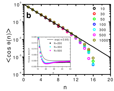
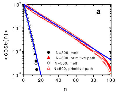
The observed swelling of long chains suggests that an evidence of remnant long-range bond-bond correlations should be detectable. Thus, we examine the intrachain orientational bond-bond correlations as a function of the internal distance . Fig. 3b represents the orientational bond-bond correlations for different chain lengths that are obtained by averaging over 500-2500 equilibrated configurations that are apart. We find that the bond-bond correlation functions of all the chain lengths decay exponentially up to and can be well described by . We extract the so-called persistence length from the bond-bond orientational correlation functions. is defined by their decay length, more precisely:
| (8) |
Using and , we obtain . Alternatively, we can estimate the persistence length from as which leads to comparable to the estimated value from fitting the bond-bond orientational correlation functions with an exponential decay. Notably, the relation valid for worm-like chains roughly holds for semiflexible CG-PVA polymers.
For larger values, similar to the MSIDs, bond-bond correlations deviate from exponential decay but we do not observe any sign of long-range power law decay reported for 3D melts of chains with zero persistence length Wittmer et al. (2004) and the semiflexible polymers with a harmonic bending potential Hsu (2014). A careful examination of the bond-bond correlations of longer chains, for which we have sufficient statistics (inset of Fig. 3b), shows that becomes slightly negative for larger values with a dip around before it decays to zero. This feature is most likely a precursor of crystallization as is slightly above the crystallization temperature. Although the negative dip in is convergent for all the three well equilibrated chain lengths, further investigations are required to establish the existence and origin of this negative dip. Especially, a better statistics is needed to calculate the error bars.
In Fig. 4, we have investigated the temperature dependence of for where the data for are obtained from cooling of the melt Meyer and Müller-Plathe (2002); Jabbari-Farouji et al. (2015b). As can be deduced from Fig. 4 at and 0.8, where the polymers are in the semicrystalline state, the negative dip is further amplified due to local backfolding of the chains. Equilibrating the polymers at higher temperature of well above , we confirm that their is strictly positive as expected. The inset of Fig. 4 depicts a log-log plot of and shows that beyond , bond-bond correlation exhibits a power law decay that is a signature of long-range chain self-interactions.
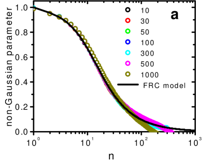
To further inspect the origin of small but systematic deviations from the FRC model, we investigate the non-Gaussian parameter of CG-PVA polymers and compare it to that of the FRC model prediction. The non-Gaussian parameter is defined in terms of second and fourth moments of internal distances and it vanishes if the internal distances are Gaussian distributed. The fourth moment of internal distances of the FRC model depends only on and Honnell et al. (1990b) where is the second Legendre polynomial. Fig. 5a presents the non-Gaussian parameter of CG-PVA polymers of different chain lengths that is compared to that of the FRC model evaluated with and extracted from simulation results. Overall, we find a good agreement between the of CG-PVA polymers and that of the FRC model. However, we notice small deviations from the FRC model for long chains and .
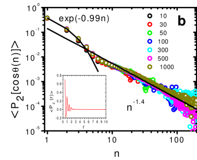
In Fig. 5b, we have plotted for different chain lengths. According to the FRC theory, should also decay exponentially as Porod (1953). We find that the initial decay of up to is well described by the FRC model predictions. However, for larger we observe important deviations from the FRC model and exhibits a clear power law behavior over more than one decade of . The observed power law behavior is a manifestation of long-range bond-bond correlations along the chain backbone that result from incomplete screening of excluded volume interactions. As noted by Meyer et. al. in the case of 2D polymer melts, it is related to the return probability after bonds and the local nematic ordering of nearby bonds Meyer et al. (2010).
To understand better the origin of this power law decay, we investigate the intrachain nematic ordering by calculating the for all bond pairs that belong to the same chain and their midpoints are a distance apart. is almost independent of chain length for . In the inset of Fig. 5b, we have presented the as a function of distance for . As can be seen, the orientational correlations oscillate and decay rapidly with . This behavior shows that for a fixed curvilinear distance only bonds which are spatially close to each other with separations contribute to . Therefore, one expects that will be directly proportional to the return probability of monomer after bonds Meyer et al. (2010) that we denote by . More precisely
| (9) |
where is the probability distribution function of the end-to-end vector of all the chain segments (subchains) with bonds.
For an ideal self-similar chain for any subchain of size follows a Gaussian distribution of the form
| (10) |
where and Rubinstein and Colby (2003); Doi and Edwards (1986). Hence, the return probability scales as . For semiflexible CG-PVA polymers with local correlations, we expect that follows Eq. 10 for . The scaling exponent that we obtain from fitting of with power law is , that is not so far from the prediction for the Gaussian chains. This small discrepancy is most likely due to insufficient statistics for large values. To test the validity of Gaussian distribution for the internal distances we examine the behavior of intrachain distributions in the subsequent subsection.
Intrachain distribution functions
Having examined the intrachain correlations, we investigate conformational behavior of chains by extracting the probability distribution of the internal distances, i.e. from the polymer configurations. As before, denotes the distance between any pair of monomers and that are bonds apart. Let us first consider the probability distribution function of bond length corresponding to . In Fig. 6a, we have shown the distribution of bond length that is independent of the chain length . The normalized distributions of bond length can be well described by a Gaussian distribution of the form
| (11) |
in which represents the standard deviation and the peak value agrees with the average bond length.
Next, we examine the probability distributions of bond angles and compare them with the form expected from the Boltzmann distribution where is a normalization constant such that . Fig. 6b presents obtained from accumulating the histograms of bond-angles and the Boltzmann distribution prediction. Overall, we find a good agreement between the two probability distribution functions for all the chain lengths.
Next, we focus on the normalized probability distribution of internal distances for and compare them to the theoretical distribution functions. The exact segmental size distribution functions of semiflexible polymers for an arbitrary are not known. However, Koyama has proposed approximate expressions for the probability distribution functions of wormlike chain model Schmidt and Stockmayer (1984) that are applicable to any semiflexible polymer model for curvilinear distances larger than the persistence segment Mansfield (1986). The Koyama distribution is constructed in such a way that it reproduces the correct second and forth moments of internal distances, i.e. and and it interpolates between the rigid-rod and the Gaussian coil limits Mansfield (1986). It is found to account rather well for the site-dependence of the intrachain structure of short CG-PVA polymers Vettorel et al. (2007).
The Koyama distribution can be expressed in terms of scaled internal distances as
| (12) |
in which and . As one would expect, at sufficiently large for which the non-Gaussian parameter vanishes, the Koyama distribution becomes identical to the Gaussian distribution valid for fully flexible ideal chains. For ideal chains, the probability distribution function of the is given by Eq. (10). As a result, the corresponding probability distribution function for the reduced internal distances, , follows from
| (13) |
where . Particularly, one expects that the distribution functions of the end-to-end distance of sufficiently long chains should follow this distribution.
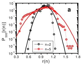
Let us first look at the distribution of internal distances for short subchains (segments). We verified the distribution of subchains does not depend on the chain length. Therefore, we focus on subchains of polymers with monomers. Fig. 7a presents for subchains comprising of and 5 bonds. As can be seen, for such short segments the features of angular potential are dominant and the Koyama distribution can not provide an accurate description of segmental size distribution although it agrees well with in the central region of the distribution and it captures accurately the height of the peaks.
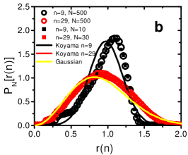
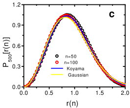
Fig. 7b shows for subchains with and 29 bonds that are larger than the persistence segment size. We note that the signature of bending potential is still visible for . Thus, the Koyama distribution does not provide a good description. For , the Koyama distribution agrees quite well with the extracted from simulations whereas the Gaussian distribution exhibits a poorer agreement. Additionally, we have included the distribution of the scaled end-to-end distance of short chains with and monomers in Fig. 7b. They coincide with the distributions of subchains with the same length. These results show that the chain-end effects, if any, are negligible and only depends on . For longer subchains and 100, depicted in Fig. 7c displays a perfect agreement with the Koyama distribution. For such long subchains, the distribution functions approach to that of a Gaussian given by Eq. (13), as one would expect.
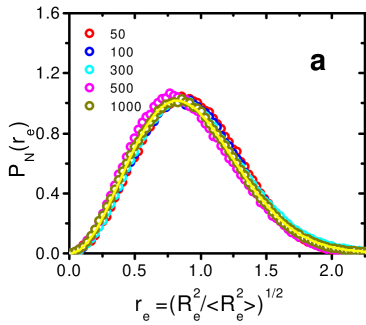
Finally, we present the normalized probability distributions of the scaled end-to-end distance for in Fig. 8a. All the data for collapse on a single master curve. We find a very good agreement between the master curves and the theoretical prediction for the -independent normalized distribution function given by Eq. (13) as demonstrated in Fig. 8a.
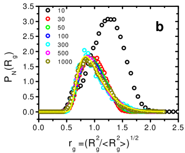
Fig. 8b shows the normalized probability distributions of the scaled gyration radius for different chain lengths. Similar to , the of chains with collapse on a single master curve. The exact expression for the probability distribution of the gyration radius is more complicated and does not have a compact form Fujita and Norisuye (1970). However, the formula suggested by Lhuillier Lhuillier (1988) for polymer chains under good solvent conditions is found to provide a good approximation for ideal chains Vettorel et al. (2010); Hsu (2014); Hsu and Kremer (2016) too. The Lhuillier formula for the scaled gyration radius in -dimensions reduces to
| (14) |
in which the exponents and are related to the space dimension and the Flory exponent by and . and are system-dependent non-universal constants and is a normalization constant such that . We find that the data of of CG-PVA polymers can be well fitted by the -independent normalized distribution function given by Eq. (14) as plotted in Fig. 8b. Having investigated the conformational properties of CG-PVA polymers, we focus on their structural properties in the Fourier space in the next subsection Vettorel et al. (2007); Meyer et al. (2010).
Form factor and structure factor
A common way to characterize the structural properties of polymer melts is to explore their structure factor that can be measured directly in the scattering experiments. The structure factor encompasses the information about spatial correlations between the monomers via Fourier transform of density-density correlation functions. For spatially homogeneous and isotropic systems such as polymer melts at equilibrium, the static structure factor only depends on the modulus of the wave vector. The static structure factor measured in scattering experiments of amorphous melts is often spherically averaged over all the wave vectors with the same modulus . This quantity can be computed as
| (15) |
where the angular brackets represent averaging over all the wave vectors with the same modulus and all the melt configurations.
given in Eq. (15) encompasses scattering from all the monomer pairs. It can be split into intrachain and interchain contributions
| (16) |
where (V volume of the simulation box) is the monomer density and
| (17) |
includes the contributions from intrachain pair correlations and it is called intrachain or single chain structure factor. Equivalently, known as the form factor Rubinstein and Colby (2003) is used to quantity the intrachain correlations in the Fourier space. The interchain contribution is given by that is defined as the Fourier transform of intermolecular pair correlation function Hansen and McDonald (1986) as
| (18) |
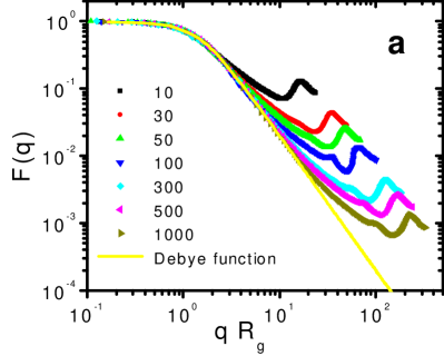
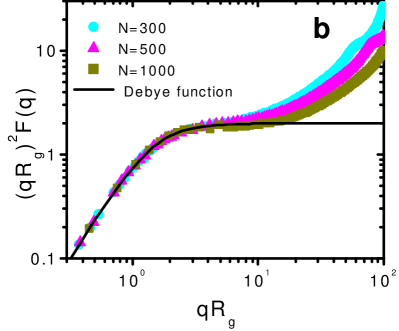
We present the behavior of the form and structure factors for different chain lengths. We first focus on the form factor as depicted in Fig. 9. The form factor of Gaussian chains, known as the Debye function, is described by Rubinstein and Colby (2003)
| (19) |
In order to compare the behavior of CG-PVA polymers in the melt state with that of ideal Gaussian chains, in Fig. 9a, we have plotted the form factor of CG-PVA chains and the Debye function versus . For all the chain lengths, we observe deviations from the ideal polymer behavior at high values. The onset of deviations shifts progressively to larger wave vectors for longer chains. For the longest chains , we have also presented the form factors in a Kratky-plot in Fig. 9b. This plot confirms the existence of a Kratky plateau in the scale free regime that extends up to for . The deviations at larger values reflect the underlying form of the bond angle potential that dominates the behavior of the form factor at length scales smaller or comparable to the Kuhn length.
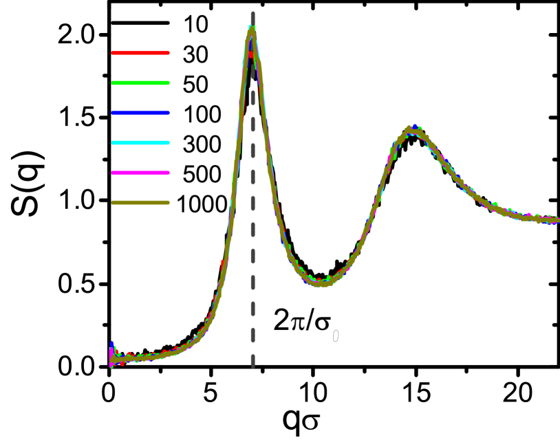
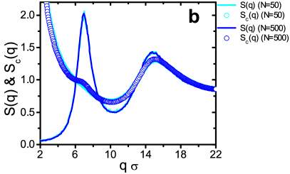
Next, we present the structure factor of different chain lengths in Fig. 10. As we notice, the of all the polymer melts displays the characteristic features of the liquid-state. We find a very weak dependence on the chain length; for , the of various chain lengths are identical. We notice several important features in the structure factors. First, the structure factor at low is very small. By virtue of compressibility equation that relates the isothermal compressibility to the structure of the liquid, i.e. , we conclude that the polymer melts are almost incompressible. Second, the first peak of at characterizes the packing of monomers in the first nearest neighbor shell. The value of nearly agrees with reflecting that the first peak of is dominated by interchain contributions.
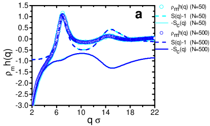
To gain more insight into the interchain correlations of CG-PVA polymers, we compare with that of simple liquids with no internal structure. For such a simple liquid, we have , hence Hansen and McDonald (1986). Fig. 11a shows both and for two chain lengths and . We find that in the region near the first peak and coincide confirming that the peak at is totally determined by the interchain correlations. In Fig. 11a, we have also included . We note that for very low wave vectors beyond the peak region, closely agrees with . This behavior shows that the correlation between monomers of different chains decreases with increasing distance. This decrease is concomitant by the increase of at low values such that the sum of both intrachain and interchain contributions yields a small finite value for as .
In the other extreme of , deviates from as the large behavior of structure factor is fully determined by the intrachain correlations due to the correlation hole effect de Gennes (1979); Vettorel et al. (2007). The correlation hole effect leads to a decreased probability of finding a monomer of another chain in the pervaded volume of a particular chain. To illustrate this point, in Fig. 11b, we have shown and for and in the same plot. We see that the large- behavior is entirely dominated by intrachain contributions. These observations are in agreement with the prior investigations for short chain lengths Vettorel et al. (2007).
Primitive path analysis and entanglement statistics
Having investigated conformational and structural features of CG-PVA polymer melts, we focus on their topological characteristics, i.e. interchain entanglements. Entanglements stem from topological constraints due to the chain connectivity and uncrossability that restrict the movements of chains at the intermediate time and length scales. As first noted by Edwards Edwards (1967), the presence of neighboring strands in a dense polymer melt effectively confines a single polymer strand to a tube-like region. The centerline of such a tube is known as the primitive path (PP). A practical and powerful method for characterizing the entanglements is primitive path analysis (PPA). Such an analysis provides us with an operational definition of primitive path and allows to investigate statistics of chain entanglements.
There exists a couple of variants of PPA in the literature Kröger (2005); R. Hoy (2009); Everaers et al. (2004) that are all similar in spirit. Here, we implement the PPA method proposed by Everaers et al. Everaers et al. (2004) that identifies the primitive path of each polymer chain in a melt based on the concept of Edwards tube model Edwards (1967). The primitive path is defined as the shortest path between the chains ends that can be reached from the initial conformations of polymers without crossing other chains. In this analysis, topologies of chains are conserved, and chains are assumed to follow random walks along their primitive paths. Therefore, the primitive path is a random walk with the same mean square end-to-end distance but shorter bond length and contour length .
In practice, by extracting the average bond length of the primitive paths , we can determine all the other desired quantities. In particular, the Kuhn length of primitive path is obtained as
| (20) |
The so-called entanglement length , defined as the average number of monomers in the Kuhn segment of the primitive path, follows from
| (21) |
Operationally, we obtain the primitive paths of polymers in a melt by slowly cooling the system toward while the two chain ends are kept fixed. During this procedure, the intrachain excluded volume interactions and bond angle potential are switched off. The system is then equilibrated using a conjugate gradient algorithm in order to minimize its potential energy and reach a local minimum. We perform primitive path analysis for the two longest chain lengths that are fully equilibrated, i.e. and 500 as it is known that poor equilibration affects the entanglement length R. Hoy (2009).
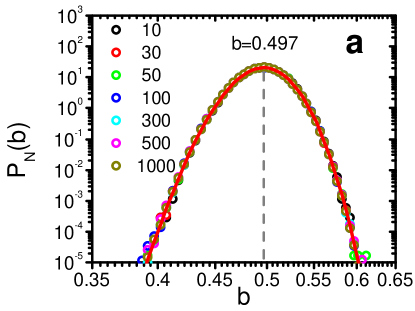
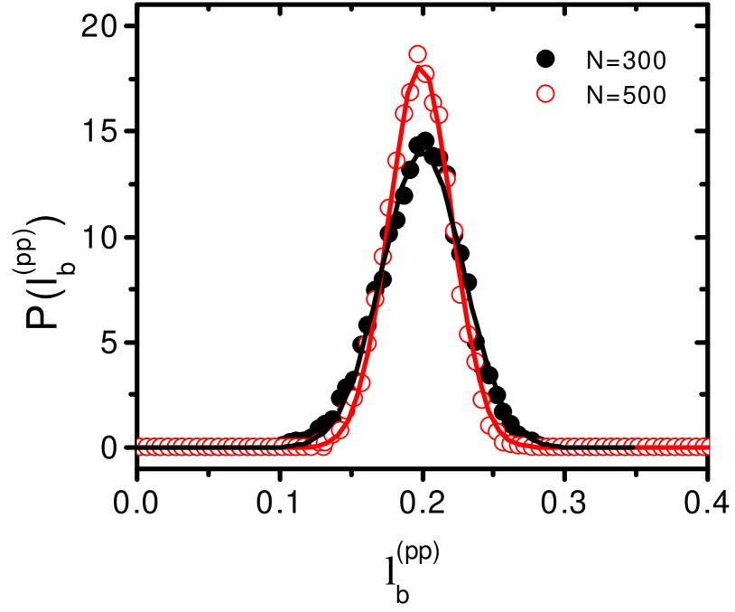
We first examine the probability distributions of the bond lengths of the primitive paths, i.e. as presented in Fig. 12. The distributions of bond lengths of the primitive paths are chain length dependent but both are centered at . Furthermore, the primitive path bond length fluctuations are considerably larger than those of their original paths. The normalized distributions of primitive path bond length can be well described by a Gaussian distribution of the form
| (22) |
where presents the -dependent standard deviation of .
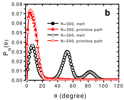
Next, we investigate the statistical features of bond angles of the primitive paths. Fig. 13a presents the bond-bond orientational correlation function as a function of internal distance for the primitive paths of chain lengths and 500. For comparison, we have also shown the of the original polymer conformations. Similar to the original polymer conformations, the initial decay of for can be well described by an exponential decay. However, at short scales , bonds are slightly stretched out because of the constraints of fixed chain ends during minimization of primitive path length. Assuming an exponential function of the form , we can extract the persistence length of the primitive path . From the fit values, we find that is considerably larger than the persistence length of the original conformations .
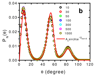
We also examine the normalized probability distributions of bond angles of the primitive paths as displayed in Fig. 13b. Unlike the bond angle distributions of the original chain conformations, the bond angles of the primitive paths is unimodal with its peak centered around . Furthermore, the range of angles shrinks from for the original paths to for the primitive paths reflecting that the primitive paths are mainly in stretched conformations.
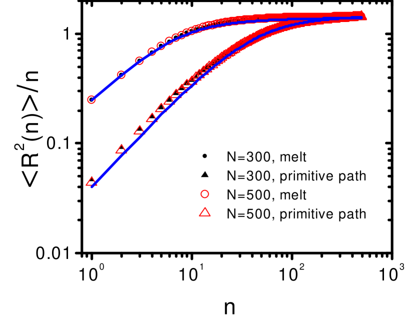
To explore the intrachain correlations of the primitive paths, we have plotted the mean square internal distances of the original and primitive paths in Fig. 14. As expected the values of for both paths approach the same value with increasing , since the chains endpoints during the primitive path analysis are held fixed. We find that results of for the primitive path can still be relatively well described by the generalized FRC model provided that we use extracted from bond-bond orientational correlations. Having confirmed that the mean end-to-end distance of the primitive paths remain identical to those of the original chains, we obtain for the Kuhn length of the primitive path. We note that the is larger than the Kuhn length of polymers .
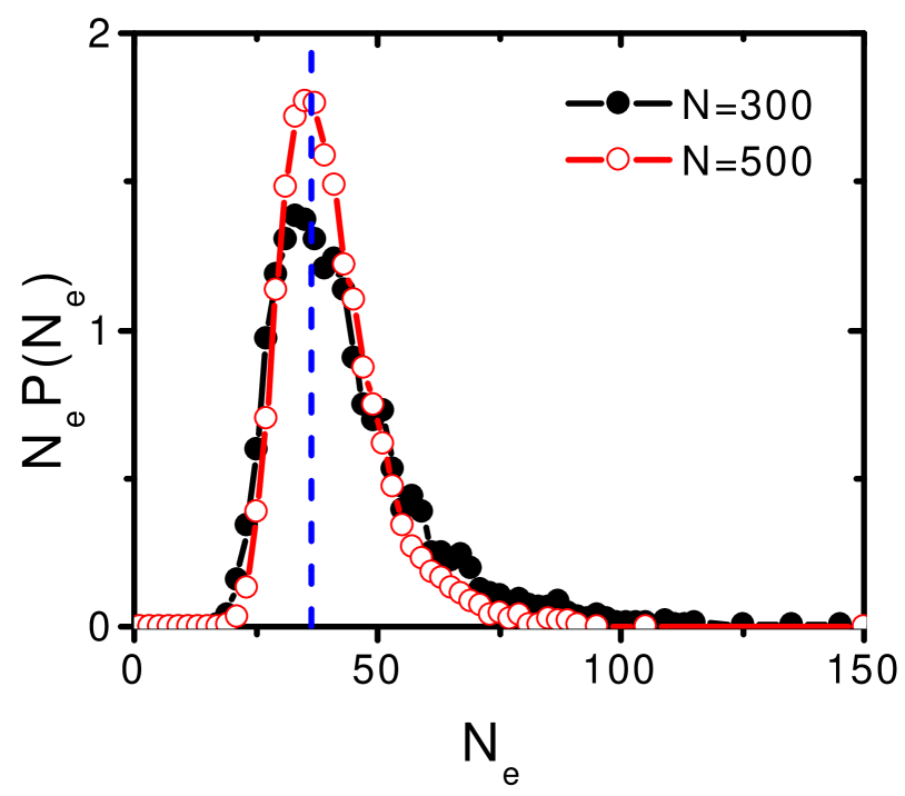
Subsequently, we acquire the distribution of entanglement length as presented in Fig. 15a. We notice that has a narrow distribution and presents a weak dependence on possibly resulting from the finite size of the chains. Our estimated value of the average entanglement length is for and for . These results suggest that we are rather close to the asymptotic value of entanglement length . We have also plotted in Fig. 15b and we find that the position of the peak of coincides with our estimated value of . This observation is in agreement with the PPA analysis results for the Kremer-Grest (FENE) model Hsu and Kremer (2016).
Dynamic scaling of monomer motion
To compare the dynamic behavior of polymer melts with the predictions of the Rouse and reptation theories Doi and Edwards (1986), we measure
the mean square displacement (MSD) of monomers for short () and long chains (). The quantities often used to characterize the segmental motion of
polymer chains in a melt are listed below.
i) the mean square displacement of inner monomers
| (23) |
where only the monomers in the central region of a chain are considered to suppress the fluctuations caused by the chain ends.
ii) the mean square displacement of inner monomers with respect to
the corresponding center of mass (c.m.) obtained as:
| (24) |
iii) the mean square displacement of the center of mass of chains defined as:
| (25) |
For short chains the topological constraints do not play a dominant role. Hence, all the interchain interactions can be absorbed into a monomeric friction and a coupling to a heat bath. The dynamics of the chain can then be described by a Langevin equation with noise and the constraint that the monomers are connected to form a chain. This description is known as the Rouse random walk model Doi and Edwards (1986); Rubinstein and Colby (2003). Beyond the microscopic timescale , the Rouse model predicts that both and scale as for timescales in which is known as the Rouse time. It corresponds to the longest relaxation time of polymers. At longer times corresponding to , is expected to follow the Fickian diffusion and scale as whereas is predicted to exhibit a plateau. The mean-square displacement of chain’s center of mass is predicted to be diffusive at all the times with the diffusion coefficient scaling as .
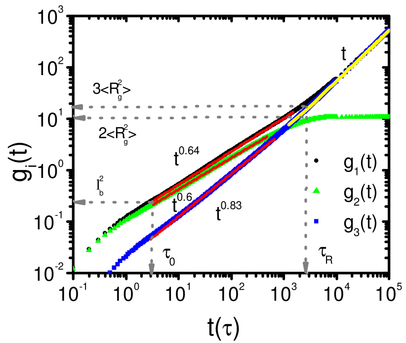
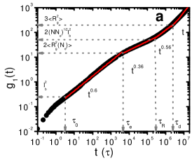
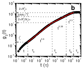
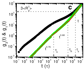
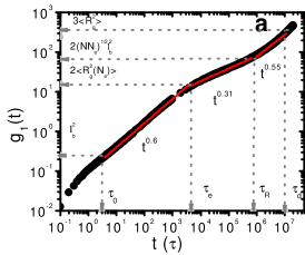
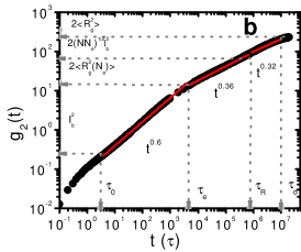
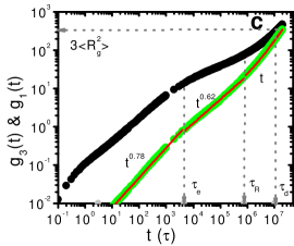
Fig. 16 presents the results of computed , and for short non-entangled polymers of chain length . The microscopic timescale is obtained as the time for which where is the Lennard-Jones (LJ) time unit. The Rouse time is estimated as . The dotted vertical lines mark the microscopic and Rouse timescales. As can be seen the Rouse timescale agrees well with the crossover points between two different scaling regimes. The horizontal dotted lines in Fig. 16 depict the values of and at . We find that and . The solid lines show the best fits with power law. For timescales smaller than a Rouse time, and exhibit a subdiffusive behavior with exponents and which are slightly higher than the Rouse random walk model scaling prediction of . The observed disagreement most likely originates from the finite persistence length of polymers. Additionally, at this regime is dominated by the crossover to the plateau. For chains with a persistence length smaller than their contour length, one expects that the monomer mean-square displacement scaling exponents to interpolate between those of the Rouse models for polymers with zero persistence length, i.e. Doi and Edwards (1986); Rubinstein and Colby (2003) and semiflexible worm-like polymers Barkema et al. (2014).
The mean square displacement of center of mass of polymers also deviates from the Rouse theory. At intermediate times , it displays an apparent power law of the form before a crossover to the expected diffusive regime. The observed subdiffusive behavior is predicted by the recent theories Farago et al. (2012, 2011) that account for the viscoelastic hydrodynamic interactions. These theories attribute the anomalous behavior of in the transient regime to incomplete screening of hydrodynamic interactions beyond the monomer length combined with the time-dependent viscoelastic relaxation of the melt. This leads to a subdiffusive motion which is not described by a pure power law; an effective exponent should decrease with chain length, but asymptotic behavior is reached extremely slowly Farago et al. (2012, 2011). Inspection of Fig. 16 shows that the data of indeed exhibits a curvature with respect to the fitted power law and the effecctive exponent of 0.83 is quite close to 1. The asymptotic dynamic scaling exponent for fully flexible chains with the Langevin dynamics is predicted to be . Considering the finite persistence length and chain size, this value is not surprising.
In long entangled polymer melts, each chain is expected to move back and forth (reptation) inside an imaginary tube with a diameter and a contour length around the so-called primitive path. Such a dynamical tube-like confinement affects the segmental motion of entangled polymers. According to the reptation theory, the dynamic scaling behavior of MSD should exhibit a crossover behavior at several timescales, the microscopic timescale , the entanglement time , the Rouse time , and the disentanglement time for long chains with . The scaling predictions of reptation theory for various time regimes are given by Doi and Edwards (1986); Kremer and Grest (1990):
| (26) |
Likewise, is predicted to show the same regimes for but to go to a plateau with a value of for . The reptation theory predicts the following scaling behavior for the polymer center of mass mean square displacement
| (27) |
To examine these scaling predictions, we compute , and for chain lengths and up to . These chain lengths include on the average 8 and 14 entanglement lengths. The results of computed , and are presented in Figs. 17 and 18. For both chain lengths, similar to the predictions of reptation theory, we observe crossovers between several scaling regimes. We first estimate the predicted crossover timescales. The microscopic timescale is identical to that for short chains. The entanglement time is estimated as the Rouse time of the chain segment between two consecutive entanglements; . Likewise the Rouse time is obtained as leading to and . The longest relaxation time determined as corresponds to and . The vertical lines in Figs. 17 and 18 mark these timescales. As can be noticed these timescales agree well with the crossover points between different scaling regimes for both chain lengths.
The horizontal dotted lines in panels a and b of Figs. 17 and 18 present the values of and at the corresponding timescales according to the reptation theory predictions. At where a Rouse chain of monomers is relaxed, the monomers displacement should be proportional to the mean squared diameter of the confining tube diameter . Assuming that and the Gaussian picture for the tube, we expect that . For where the entanglement effects set in, monomer motions are restricted to movements along the contour of the confining tube with a contour length until reaching the Rouse timescale . Since the tube itself is a random walk with a step length , the displacement of a monomer at is . For , the dynamics of is expected to crossover to a second regime which corresponds to the diffusion of the whole chain inside the tube-like region. After reaching the disentanglement time (reptation time) a chain has moved a distance comparable to its own size . The initial tube is completely destroyed and a new tube-like regime reappears. We find a good agreement between the measured values of and at various crossover timescales and the predictions of the reptation theory.
Having determined the crossover time and length scales, we obtain the dynamic exponents at various scaling regimes. The best fits of and with power laws are shown by solid lines in Figs. 17 and 18. In the first scaling regime, , we find that and the scaling exponent is larger than . This difference could again be attributed to the finite persistence length of chains as is not large enough to fall in the random walk regime. In the second regime , the obtained exponents of and are 0.36 and 0.38 for and 0.31 and 0.35 for . These values are noticeably larger than the predicted exponent. These deviations are probably because chains are not long enough to fully develop this reptation regime. These results suggest that much longer chains with are needed to observe the predicted exponent in the asymptotic limit Pütz et al. (2000). Nevertheless, upon increasing the chain length, the obtained exponents for the second scaling regime slightly improve. In the third regime, , and the exponents of both chain lengths are slightly larger than . In this regime, for and for . Unlike the theoretical predictions scaling significantly differs from that of . This discrepancy is also most likely because is not sufficiently large; the fit region includes the broad crossover to the asymptotic plateau. At the disengagement time, we find that the relation roughly holds. For , we can observe the free diffusion regime of beyond where and for the , we observe the expected plateau value of for nearly two third of a decade. For , much longer simulation times are required to obtain reliable results for .
Finally, we examine the scaling behavior of the mean square displacement of the center of mass of polymers. In contrast to the predictions of reptation theory, we observe two distinct scaling regimes for . The first one corresponds to where exhibits a subdiffusive behavior with for and for . Similar to the short chains, this subdiffusive behavior results from the coupling to time-dependent viscoelatic relaxation of the melt background Farago et al. (2012, 2011). At timescales , we observe a second scaling regime where for and for . These exponents again are notably larger than the theoretical predictions due to the finite size of the chains, but as expected, they systematically decrease with chain length.
Conclusions
We have investigated the static and dynamic properties of polymer melts of a locally semiflexible bead-spring model known as the CG-PVA model Meyer and Müller-Plathe (2001, 2002). The main distinctive feature of this model system is a triple-well bending potential that leads to polymer crystallization upon cooling of the melt. We have equilibrated polymer melts with chain lengths . The results for the long chains allow us to determine the Kuhn length , the persistence length and the entanglement length of the model polymers accurately as summarized in Table II. We note that the relation holds for the semiflexible CG-PVA polymers.
| = | ||||
|---|---|---|---|---|
We have also examined the validity of Flory’s ideality hypothesis for this model system. Our detailed examination shows that the conformations of CG-PVA polymers agree with many of the theoretical predictions for ideal chains. Notably, long polymer melts with follow the scaling relations and valid for ideal chains. The probability distribution functions of the reduced end-to-end distance and the reduced gyration radius for chain lengths also collapse on universal master curves that are well described by the theoretical distributions for the ideal chains.
Investigating the intrachain correlations, we find evidences for deviations from ideality. However, these non-Gaussian corrections are rather small and do not affect most of the large-scale conformational features. The mean square internal distances of short chains show an excellent agreement with the predictions of the generalized freely rotating chain model Flory (1969) whereas those of longer chains are slightly larger. The observed swelling of longer chains reflects an incomplete screening of excluded volume interactions and is most likely related to the correlation hole effect de Gennes (1979); Wittmer et al. (2007a). We also compare the non-Gaussian parameter of CG-PVA polymers with that of the freely rotating chain model. The agreement is rather good and we only observe some small deviations for long chains.
Carefully examining the bond-bond correlations of long chains at , we do not observe any long-range bond-bond correlations. Instead, the triple-well angle-bending potential leads to weak anti-correlations for curvilinear distances of about . The observed anti-correlation is a precursor of chain backfolding in the melt at temperatures slightly above the crystallization temperature. This feature is further enhanced in the semicrystalline state and it is a signature of chain-folded structures Meyer and Müller-Plathe (2002); Jabbari-Farouji et al. (2015b). The anti-correlations suppress long-range bond-bond correlations but the long-range intrachain correlations are visible in the second Legendre polynomial of the cosine of angles between the bonds, , that exhibit a power law decay in analogy to the reports for 2D polymer melts Meyer et al. (2010).
Moreover, we have investigated in detail the intrachain and interchain structure factors of different chain lengths. The interchain structure factor is almost independent of the chain length whereas the intrachain structure factor depends on as expected. We find that of sufficiently long CG-PVA polymer are well-described by the Debye function for length scales larger than the Kuhn length. The agreement with the Debye function improves upon increase of . Notably, we observe a plateau in the Kratky plot for the range . Our results are in contrast with the findings for fully flexible chains that exhibit significant deviations from the Debye function at intermediate wave-vectors Wittmer et al. (2007a); Beckrich et al. (2007); Hsu (2014). But, they agree with the recent findings that increasing the bending stiffness of the chains in a melt, irrespective of details, improves the agreement with the ideal-chain limit Hsu and Kremer (2016).
Using the primitive path analysis, we have determined the average entanglement length of long and equilibrated chains and we have compared the original polymer paths with their primitive paths. Probing the bond-bond orientational correlation function and the mean square internal distance of primitive paths, we confirm the assumption that polymers behave nearly as Gaussian chains along their primitive paths. Notably, the Kuhn length of the primitive path is more than twice the of the original path. The average bond length of primitive paths follows a Gaussian distribution and the peak of the first moment of the entanglement length probability distribution agrees with the average entanglement length.
Investigating the segmental motion of entangled polymer melts, we observe several scaling regimes as predicted by the reptation theory. The crossover time and length scales between distinct scaling regimes agree with the predictions of the reptation theory Doi and Edwards (1986); Kremer and Grest (1990). However the dynamical exponents of monomer mean square displacements are different from those of the theory most probably due to the finite persistence length and size of polymers. The mean square displacement of center of mass of polymers also exhibits an anomalous diffusion at the timescale where the Rouse and reptation theories predict a Fickian diffusion. However, our results are qualitatively consistent with the more recent theories Farago et al. (2012, 2011) that attribute the subdiffusive motion of polymers center of mass to viscoelastic hydrodynamic interactions. It still remains an open question, how a finite persistence length of polymers affects quantitatively the dynamic exponents of center of mass particularly in the reptation regime.
acknowledgments
S. J.-F. is grateful to Jean-Louis Barrat Hendrik Meyer, Kurt Kremer and Hsiao-Ping Hsu for insightful discussions. She also acknowledges financial support from the German Research Foundation (http://www.dfg.de) within SFB TRR 146 (http://trr146.de). The computations were performed using the Froggy platform of the CIMENT infrastructure supported by the Rhone-Alpes region (Grant No. CPER07-13 CIRA) and the Equip@Meso Project (Reference 337 No. ANR-10-EQPX-29-01) and the supercomputer clusters Mogon I and II at Johannes Gutenberg University Mainz (hpc.uni-mainz.de).
References
- Rubinstein and Colby (2003) M. Rubinstein and R. H. Colby, Polymer Physics (Oxford University Press, Oxford, 2003).
- Mandelkern (1990) L. Mandelkern, Accounts of Chemical Research 23, 380 (1990), https://doi.org/10.1021/ar00179a006 .
- Keller (1968) A. Keller, Reports on Progress in Physics 31, 623 (1968).
- edited by J.-U. Sommer and Reiter (2003) edited by J.-U. Sommer and G. Reiter, Lecture Notes in Physics 606 (2003).
- Flory (1956) P. Flory, Proceedings of the Royal Society of London A: Mathematical, Physical and Engineering Sciences 234, 60 (1956).
- Olmsted et al. (1998) P. D. Olmsted, W. C. K. Poon, T. C. B. McLeish, N. J. Terrill, and A. J. Ryan, Phys. Rev. Lett. 81, 373 (1998).
- Sushko et al. (2001) N. Sushko, P. van der Schoot, and M. A. J. Michels, The Journal of Chemical Physics 115, 7744 (2001).
- McCoy et al. (1991) J. D. McCoy, K. G. Honnell, K. S. Schweizer, and J. G. Curro, The Journal of Chemical Physics 95, 9348 (1991).
- Oxtoby (2002) D. W. Oxtoby, Annu. Rev. Mater. Res. 32, 39 (2002).
- Meyer and Müller-Plathe (2001) H. Meyer and F. Müller-Plathe, The Journal of Chemical Physics 115, 7807 (2001).
- Reith et al. (2001) D. Reith, H. Meyer, and F. Müller-Plathe, Macromolecules 34, 2335 (2001), https://doi.org/10.1021/ma001499k .
- Jabbari-Farouji et al. (2015a) S. Jabbari-Farouji, J. Rottler, O. Lame, A. Makke, M. Perez, and J. L. Barrat, ACS Macro Letters 4, 147 (2015a).
- Jabbari-Farouji et al. (2017) S. Jabbari-Farouji, O. Lame, M. Perez, J. Rottler, and J.-L. Barrat, Phys. Rev. Lett. 118, 217802 (2017).
- Triandafilidi et al. (2016) V. Triandafilidi, J. Rottler, and S. G. Hatzikiriakos, Journal of Polymer Science Part B: Polymer Physics , 2318 (2016).
- Luo and Sommer (2013) C. Luo and J. Sommer, ACS Macro Letters 2, 31 (2013).
- Luo and Sommer (2016) C. Luo and J.-U. Sommer, ACS Macro Letters 5, 30 (2016).
- Vettorel et al. (2007) T. Vettorel, H. Meyer, J. Baschnagel, and M. Fuchs, Phys. Rev. E 75, 041801 (2007).
- Flory (1969) P. J. Flory, Statistical Mechanics of Chain Molecules (Wiley, New York, 1969).
- Doi and Edwards (1986) M. Doi and S. F. Edwards, The Theory of Polymer Dynamics (Clarendon Press, Oxford, 1986).
- Wittmer et al. (2004) J. P. Wittmer, H. Meyer, J. Baschnageland, A. Johner, S. Obukhov, L. Mattioni, M. Muller, and A. N. Semenov, Physical Review Letters 93, 147801 (2004).
- Wittmer et al. (2007a) J. P. Wittmer, P. Beckrich, A. Johner, A. N. Semenov, S. Obukhov, H. Meyer, and J. Baschnagel, Europhysics Letters 77, 56003 (2007a).
- Wittmer et al. (2007b) J. P. Wittmer, P. Beckrich, H. Meyer, A. Cavallo, A. Johner, and J. Baschnagel, Physical Review E 76, 011803 (2007b).
- Beckrich et al. (2007) P. Beckrich, A. Johner, A. N. Semenov, S. P. Obukhov, H. C. Benoit, and J. P. Wittmer, Macromolecules 40, 3805 (2007).
- Hsu (2014) H.-P. Hsu, J. Chem. Phys. 141, 164903 (2014).
- Semenov (2010) A. N. Semenov, Macromolecules 43, 9139 (2010).
- Hsu and Kremer (2016) H.-P. Hsu and K. Kremer, J. Chem. Phys. 144, 154907 (2016).
- de Gennes (1979) P. G. de Gennes, Scaling Concepts in Polymer Physics (Cornell University Press, Itharca, New York, 1979).
- Meyer and Müller-Plathe (2002) H. Meyer and F. Müller-Plathe, Macromolecules 35, 1241 (2002).
- Jabbari-Farouji et al. (2015b) S. Jabbari-Farouji, J. Rottler, O. Lame, A. Makke, M. Perez, and J. L. Barrat, Journal of Physics: Condensed Matter 27, 194131 (2015b).
- Plimpton (1995) S. Plimpton, Journal of Computational Physics 117, 1 (1995).
- Honnell et al. (1990a) K. G. Honnell, J. G. Curro, and K. S. Schweizer, Macromolecules 23, 3496 (1990a).
- Honnell et al. (1990b) K. G. Honnell, J. G. Curro, and K. S. Schweizer, Macromolecules. 23, 3496 (1990b).
- Porod (1953) G. Porod, Journal of Polymer Science 10, 157 (1953).
- Meyer et al. (2010) H. Meyer, J. P. Wittmer, T. Kreer, A. Johner, and J. Baschnagel, The Journal of Chemical Physics 132, 184904 (2010).
- Schmidt and Stockmayer (1984) M. Schmidt and W. Stockmayer, Macromolecules 17, 509 (1984).
- Mansfield (1986) M. L. Mansfield, Macromolecules 19, 854 (1986).
- Fujita and Norisuye (1970) H. Fujita and T. Norisuye, J. Chem. Phys. 52, 1115 (1970).
- Lhuillier (1988) D. Lhuillier, J. Phys. France 49, 705 (1988).
- Vettorel et al. (2010) T. Vettorel, G. Besold, and K. Kremer, Soft Matter 6, 2282 (2010).
- Hansen and McDonald (1986) J. P. Hansen and I. R. McDonald, Theory of Simple Liquids (Academic Press, London, 1986).
- Edwards (1967) S. F. Edwards, Proc. Phys. Soc. 91, 513 (1967).
- Kröger (2005) M. Kröger, Comput. Phys. Commun. 168, 209 (2005).
- R. Hoy (2009) M. K. R. Hoy, K. Foteinopoulou, Phys. Rev. E 80, 031803 (2009).
- Everaers et al. (2004) R. Everaers, S. K. Sukumaran, G. S. Grest, C. Svaneborg, A. Sivasubramanian, and K. Kremer, Science 303, 823 (2004).
- Barkema et al. (2014) G. T. Barkema, D. Panja, and J. M. J. van Leeuwen, Journal of Statistical Mechanics: Theory and Experiment 2014, P11008 (2014).
- Farago et al. (2012) J. Farago, H. Meyer, J. Baschnagel, and A. N. Semenov, Phys. Rev. E 85, 051807 (2012).
- Farago et al. (2011) J. Farago, H. Meyer, and A. N. Semenov, Phys. Rev. Lett. 107, 178301 (2011).
- Kremer and Grest (1990) K. Kremer and G. S. Grest, J. Chem. Phys. 92, 5057 (1990).
- Pütz et al. (2000) M. Pütz, K. Kremer, and G. S. Grest, EPL (Europhysics Letters) 49, 735 (2000).