Asymmetric Mach-Zehnder atom interferometers

Abstract

It is shown that using beam splitters with non-equal wave vectors results in a new recoil diagram which is qualitatively different from the well-known diagram associated with the Mach-Zehnder atom interferometer. We predict a new asymmetric Mach-Zehnder atom interferometer (AMZAI) and study it when one uses a Raman beam splitter. The main feature is that the phase of AMZAI contains a quantum part proportional to the recoil frequency. A response sensitive only to the quantum phase was found. A new technique to measure the recoil frequency and fine structure constant is proposed and studied outside of the Raman-Nath approximation.

It is well-known that atom interferometry c1 is caused by the quantization of the atomic center-of-mass motion. When the incident atomic momentum state $\left|\mathbf{p}\right\rangle$ splits into two states $\left|\mathbf{p}\right\rangle$ and $\left|\mathbf{p}+\hbar\mathbf{k}\right\rangle$ after passing through a beam splitter having effective wave vector $\mathbf{k},$ the coherence between these states evolves as

$$\rho\left(\mathbf{p}+\hbar\mathbf{k},\mathbf{p},t\right)\propto\exp\left(-i\omega_{\mathbf{p}+\hbar\mathbf{k},\mathbf{p}}t\right)$$ (1)

where the frequency of transition between states

$$\omega_{\mathbf{p}+\hbar\mathbf{k},\mathbf{p}}=\dfrac{1}{2M\hbar}\left[\left(\mathbf{p}+\hbar\mathbf{k}\right)^{2}-\mathbf{p}^{2}\right]=\mathbf{k}\cdot\dfrac{\mathbf{p}}{M}+\dfrac{\hbar\mathbf{k}^{2}}{2M}$$ (2)

contains the quantum term, recoil frequency

$$\omega_{k}=\dfrac{\hbar\mathbf{k}^{2}}{2M},$$ (3)

where $M$ is an atomic mass. When $t$ is of the order of interrogation time $T$ of the given atomic interferometer, one can expect the phase of the interferometer to contain the quantum contribution

$$\phi_{q}\thicksim\omega_{k}T,$$ (4)

which would reveal the quantum nature of the atom interference. This phase leads to the recoil splitting of the optical Ramsey fringes c16 , Talbot effect, i.e. quantum beats of the atom interferometer signal, in the standing wave fields c1 ; c17 ; c20 and microfabricated structures c18 . Precise measurement of the phase (4) was performed c9 using a Raman analogue of the atom interferometer c19 involving 4 time-separated counterpropagating traveling waves. The value of $\omega_{k}$ was proposed for measuring the fine structure constant c9 , which resulted c14 in a resolution in this constant of 0.25 ppb.

In spite of this, the phase of the well-known and widely used Mach-Zehnder atom interferometer (MZAI), in which an atom passes through 3 beam splitters separated in time with a delay $T$, contains no quantum term. In the uniform gravitational field $\mathbf{g}$ the phase is given by c2

$$\phi=\mathbf{k}\cdot\mathbf{g}T^{2}.$$ (5)

The reason is that quantum corrections affect the atomic position at the moments of interaction with the 2nd and 3rd beam splitters, but in the uniform gravity field these contributions cancel one another (see for example Appendix in c3 ). We would like to underline that derivations of the MZAI phase is purely quantum (see examples of this derivation in c2 ; c3 ; c4 ),but the result of those derivations (5) is purely classical. The quantum contribution to the MZAI phase arises in the rotating frame c4.1 , or in the non-uniform field, in the presence of the gravity-gradient tensor c4.2 ; c8 or in the presence of the gravity curvature tensor c3 , or in the strongly non-uniform field of the external test mass c3 , the quantum part of the phase in gravity-gradient field of the external test mass has been recently observed c33 .

The absence of the quantum phase (4) allows one to doubt that MZAI is caused by matter wave interference. In this article, I propose a modification of the MZAI which contains the term (4). Moreover, we found a response that contains only the quantum phase. Since it is insensitive to gravity, vibration, phase and frequency noise, this response can be used to measure recoil frequency and fine structure constant. An advantage of our approach compared to the approach, using conjugate atom interferometers in the Bragg regime c3.1 , is that our effect is insensitive to phase and frequency noise and has no diffraction phase c3.2 .

In our modification, we first tried to use beam splitters with different effective wave vectors. If the beam splitter is a pulse of standing wave c1 , or Raman pulse c4 , then usually the field consists of two counterpropagating traveling waves having wave vectors $\mathbf{q}_{1}$ and $\mathbf{q}_{2}\approx-\mathbf{q}_{1}.$ The effective wave vector of this beam splitter is

$$\mathbf{k}=\mathbf{q}_{1}-\mathbf{q}_{2}\approx 2\mathbf{q}_{1}.$$ (6)

One can obtain a value of $\mathbf{k}$ different from that given by Eq. (6) if the traveling waves are not counterpropagating $\left(\mathbf{q}_{1}\not=-\mathbf{q}_{2}\right).$ In this case, the magnitude of the effective wave vector $\left|\mathbf{k}\right|=k\sin\alpha,$ where $\alpha$ is the half-angle between vectors $\mathbf{q}_{1}$ and $\mathbf{q}_{2}$ and $k\approx 2q_{1}.$ Such a field was used for the first observation of atomic focusing c5 , in the theory of conical lens for atoms c6 , to consider quasiperiodic Fresnel atom optics c7 , to separate in time double-loop atomic gyro and stimulated echo c8 . Another way of getting non-equal wave vectors is to use the sequential technique c9 ; c10 to increase $\mathbf{k}$ and apply it with different amounts of additional $\pi-$pulses near the 1st, 2nd and 3rd pulses. The sequential technique c10 is more promising than technique combining Bragg diffraction and Bloch oscillations c14 . We are expecting that AMZAI effective wave  vectors can be increased using the sequential technique and do not consider the Bloch oscillations in this article. MZAI with a slightly different effective wave vector of the second Raman pulse has been also proposed c10.1 to vanish sensitivity to the atom clouds’ initial position and the velocity caused by the gravity-gradient tensor. This effect has been recently observed c10.2 ; c10.3 . The difference from our case is that (a) we allow an arbitrary change of the wave vectors’ magnitudes, (b) but we do not violate the phase-matching conditions, (c) the gravity field is uniform (on this stage we neglect the gravity gradient terms), (d) the asymmetry proposed in c10.1 does not lead and is not aimed at leading to any quantum term in the MZAI phase.

The recoil diagram of the MZAI with non-equal wave vectors is shown in Fig. 1. Calculations show that the phase of this interferometer still has no quantum part (see appendix A).

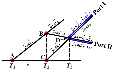
Figure 1: MZAI with different effective wave vectors. If $\left|\mathbf{p}\right\rangle$ is an incident momentum state, then the beam splitter produces, in addition to state $\left|\mathbf{p}\right\rangle,$ the scattered momentum state $\left|\mathbf{p}\pm\hbar\mathbf{k}_{i}\right\rangle$. The scattered momentum states after the 3rd beam splitter are shown in blue.

Nevertheless, one notices that lines $AB$ and $CD$ are no longer parallel, and at some moment in time they cross one another. Applying at that time the 3rd beam splitter, one obtains new an asymmetric Mach-Zehnder atom interferometer (AMZAI). One can say the same thing about lines $AC$ and $BD.$ The corresponding recoil diagram for this interferometer is shown in Fig. 2.

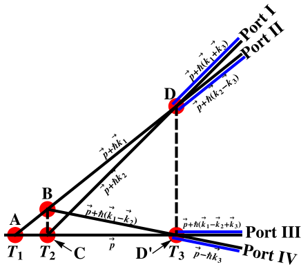
Figure 2: Recoil diagram of the AMZAI.

It is evident from the figure that the choice of the wave vectors and times $T_{i}$ has to obey 2 constraints. The first constraint is that the blue and black lines in each port have to be parallel, i.e.

$$\mathbf{k}_{1}=\mathbf{k}_{2}-\mathbf{k}_{3},$$ (7)

which is a well-known phase matching condition. The second constraint is that $D$ is the point of crossing and therefore $\overrightarrow{AD}=\overrightarrow{AC}+\overrightarrow{CD},$ which means that

$$\mathbf{k}_{1}\left(T_{3}-T_{1}\right)=\mathbf{k}_{2}\left(T_{3}-T_{2}\right).$$ (8)

One can get the same equality from the constraint $\overrightarrow{AD^{\prime}}=\overrightarrow{AB}+\overrightarrow{BD^{\prime}}.$ Choosing the wave vector $\mathbf{k}_{2}$ as an independent variable, one can get from constraints (7,8) that other wave vectors have to be equal to

$$\mathbf{k}_{1} = \left(1-s\right)\mathbf{k}_{2},$$ (9a)

$$\mathbf{k}_{3} = s\mathbf{k}_{2},$$ (9b)

where

$$s=\left(T_{2}-T_{1}\right)/\left(T_{3}-T_{1}\right).$$ (10)

If one uses a Raman pulse for beam splitting, then the change of momentum is accompanied by a change of the atomic internal states $\left|g\right\rangle$ (ground) and $\left|e\right\rangle$ (excited). Specifically, the incident state $\left|g,\mathbf{p}\right\rangle$ splits into states $\left|g,\mathbf{p}\right\rangle$ and $\left|e,\mathbf{p}+\hbar\mathbf{k}\right\rangle,$ while the incident state $\left|e,\mathbf{p}\right\rangle$ splits into states $\left|e,\mathbf{p}\right\rangle$ and $\left|g,\mathbf{p}-\hbar\mathbf{k}\right\rangle$. From the recoil diagram corresponding to these rules shown in Fig. 3, one finds in each of the output ports different atomic internal states which cannot interfere with each other.

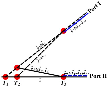
Figure 3: AMZAI in the case of Raman beam splitter for colinear beam spliters $\mathbf{k}_{1}\|\mathbf{k}_{2}\|\mathbf{k}_{3}$ and $k_{2}>k_{1}.$ Solid and dashed lines correspond to the atomic ground and excited states.

A similar situation occurs for a Stern-Gerlach beam splitter, where the use of an additional microwave pulse changes the internal atomic label and leads to interference c11 . I also propose applying here the microwave pulse resonant to transition $g\rightarrow e$ just before (the case considered here) or after 3rd Raman pulse c11.1 . It is easier to perform calculations than to draw the recoil diagram corresponding to this set of pulses.

Let’s assume that atoms are launched at $t=0$ and interact with 3 Raman pulses. Pulse $i$ is applied at time $T_{i}$ and has the area, effective wave vector, phase and Raman detuning $\theta_{i},\mathbf{k}_{i},\phi_{i}$ and $\delta_{i}$. In addition the microwave pulse, having the area, effective wave vector, phase and detuning $\theta_{m},\mathbf{k}_{m}=0,\phi_{m}$ and $\delta_{m}$, is applied at time $T_{m}.$ I assume, for simplicity, that all pulses have the same duration $\tau.$ The calculations were performed using Wigner representation for the atomic density matrix. To get the AMZAI phase, I used equations for the density matrix evolution in times between pulses and equations for the density matrix change immediately after the interaction with a given pulse, i.e. Eqs. (21, 48) in c8 . Regarding the microwave pulse time $T_{m},$ I assume that

$$0<T_{3}-T_{m}\ll T_{3}$$ (11)

so that one can ignore the density matrix evolution at $T_{m}+\tau<t<T_{3}$. If initially all atoms are in the ground state,

$$\rho_{gg}\left(\mathbf{x},\mathbf{p},0\right)=f\left(\mathbf{x},\mathbf{p}\right),\rho_{ee}\left(\mathbf{x},\mathbf{p},0\right)=\rho_{eg}\left(\mathbf{x},\mathbf{p},0\right)=0,$$ (12)

then I calculate the probability of atoms’ excitation immediately at time $T_{3}+\tau$

$$w=\int d\mathbf{p}d\mathbf{x}\rho_{ee}\left(\mathbf{x},\mathbf{p},T_{3}+\tau\right).$$ (13)

The straightforward, but extended, calculations of response (13) will be omitted here. The interaction which I consider here is a particular case of the interaction with 4 pulses considered previously in Sec. VII of the article c8 , where the 3rd pulse is a microwave pulse, the 4th pulse becomes the 3rd one, and the processes shown in Fig. 2 correspond to processes called in c8 ”stimulated echo”. Saving only these processes and background terms one finds

$$w = \bar{w}+w_{I+}+w_{I-}+w_{II+}+w_{II-},$$ (14a)

$$\bar{w} = \dfrac{1}{2}\left(1-\cos\theta_{1}\cos\theta_{2}\cos\theta_{m}\cos\theta_{3}\right),$$ (14b)

$$\left\{\begin{array}[]{c}w_{I\pm}\\ w_{II\pm}\end{array}\right\} = -\dfrac{1}{8}\sin\theta_{3}\sin\theta_{m}\sin\theta_{2}\sin\theta_{1}\int d\mathbf{x}d\mathbf{p}f\left(\mathbf{x},\mathbf{p}\right)\left\{\begin{array}[]{c}\cos\left(\phi_{I\pm}+\phi_{I}\right)\\ \cos\left(\phi_{II\pm}+\phi_{II}\right)\end{array}\right\},$$ (14g)

$$\phi_{I,II} = -\delta_{3}T_{3}+\delta_{m}T_{m}\pm\delta_{2}T_{2}\mp\delta_{1}T_{1}-\phi_{3}+\phi_{m}\pm\phi_{2}\mp\phi_{1}-\arg\left(\Omega_{3}^{\ast}\Omega_{m}\right)\mp\arg\left(\Omega_{2}\Omega_{1}^{\ast}\right),$$ (14h)

$$\left\{\begin{array}[]{c}\phi_{I\pm}\\ \phi_{II\pm}\end{array}\right\} = \left\{\begin{array}[]{c}\mathbf{k}_{3}\cdot\mathbf{x}_{3\pm}-\mathbf{k}_{2}\cdot\mathbf{x}_{2}+\mathbf{k}_{1}\cdot\mathbf{x}_{1}\\ \mathbf{k}_{3}\cdot\mathbf{x}_{3\pm}+\mathbf{k}_{2}\cdot\mathbf{x}_{2}-\mathbf{k}_{1}\cdot\mathbf{x}_{1}\end{array}\right\},$$ (14m)

$$\left\{\mathbf{x}_{1},\mathbf{p}_{1}\right\} = \left\{\mathbf{X}\left(\mathbf{x},\mathbf{p},T_{1}\right),\mathbf{P}\left(\mathbf{x},\mathbf{p},T_{1}\right)+\dfrac{\hbar\mathbf{k}_{1}}{2}\right\},$$ (14n)

$$\left\{\mathbf{x}_{2},\mathbf{p}_{2\pm}\right\} = \left\{\mathbf{X}\left(\mathbf{x}_{1},\mathbf{p}_{1},T_{2}-T_{1}\right),\mathbf{P}\left(\mathbf{x}_{1},\mathbf{p}_{1},T_{2}-T_{1}\right)\mp\dfrac{\hbar\mathbf{k}_{2}}{2}\right\},$$ (14o)

$$\mathbf{x}_{3\pm} = \mathbf{X}\left(\mathbf{x}_{2},\mathbf{p}_{2\pm},T_{3}-T_{2}\right),$$ (14p)

where $$\Omega_{n} n, \Omega_{m} \left\{\mathbf{X}\left(\mathbf{x},\mathbf{p},t\right),\mathbf{P}\left(\mathbf{x},\mathbf{p},t\right)\right\} \left\{\mathbf{x},\mathbf{p}\right\} \mathbf{g}$$ is a two-photon Raman Rabi frequency of the Raman pulse  is a Rabi frequency of the microwave pulse, is a point of the atom trajectory in the phase space, and is the initial point of this trajectory. I consider here for simplicity only atom motion in the uniform gravity field , when

$$\mathbf{X}\left(\mathbf{x},\mathbf{p},t\right) = \mathbf{x}+\dfrac{\mathbf{p}}{M}t+\mathbf{g}\dfrac{t^{2}}{2},$$ (15a)

$$\mathbf{P}\left(\mathbf{x},\mathbf{p},t\right) = \mathbf{p}+M\mathbf{g}t.$$ (15b)

Using these dependencies one obtains

$$\phi_{I\pm} = \left(\mathbf{k}_{3}-\mathbf{k}_{2}+\mathbf{k}_{1}\right)\cdot\mathbf{x}+\left(\mathbf{k}_{3}T_{3}-\mathbf{k}_{2}T_{2}+\mathbf{k}_{1}T_{1}\right)\cdot\dfrac{\mathbf{p}}{M}+\dfrac{1}{2}\left(\mathbf{k}_{3}T_{3}^{2}-\mathbf{k}_{2}T_{2}^{2}+\mathbf{k}_{1}T_{1}^{2}\right)\cdot\mathbf{g}$$ (16)

$$+\dfrac{\hbar}{2M}\left\{\mathbf{k}_{3}\cdot\left[\mathbf{k}_{1}\left(T_{2}-T_{1}\right)+\left(\mathbf{k}_{1}\mp\mathbf{k}_{2}\right)\left(T_{3}-T_{2}\right)\right]-\mathbf{k}_{2}\cdot\mathbf{k}_{1}\left(T_{2}-T_{1}\right)\right\}$$

One sees that, owing to the first two terms in Eq. (16), the integrand for $w_{I\pm}$ in Eq. (14g) rapidly oscillates in the phase space, which can wash out the interference signal.. However, owing to the constraints (7, 8) the first two terms are exactly equal to 0. Substituting Eq. (9) into Eq. (16), one finds

$$\phi_{I\pm} = \phi_{c}\mp\phi_{q},$$ (17a)

$$\phi_{c} = \dfrac{1}{2}\mathbf{k}_{2}\cdot\mathbf{g}\left(T_{3}-T_{1}\right)^{2}s\left(1-s\right),$$ (17b)

$$\phi_{q} = \omega_{k_{2}}\left(T_{3}-T_{1}\right)s\left(1-s\right).$$ (17c)

One can find that for wave vectors (9), terms $$w_{II\pm} w_{I+}+w_{I-} \phi_{c},~{}\phi_{i},~{}\delta_{i}T_{j},$$ are washed out and the sum of the interference terms contains separately a factor depending on the quantum phase (17c) and a factor depending on the all the other phases, i.e.

$$w=\bar{w}-\dfrac{1}{4}\sin\theta_{3}\sin\theta_{m}\sin\theta_{2}\sin\theta_{1}\cos\left(\phi_{q}\right)\cos\left(\phi_{c}+\phi_{I}\right),$$ (18)

If one monitors the signal (18) as a function of any phase or detuning of the Raman or microwave field, then the difference of the maximum and minimum of the signal is given by

$$A=w_{\max}-w_{\min}=\dfrac{1}{2}\left|\sin\theta_{3}\sin\theta_{m}\sin\theta_{2}\sin\theta_{1}\cos\left(\phi_{q}\right)\right|.$$ (19)

The oscillating dependence in (19) on the interrogation time $T_{3}-T_{1}$ is caused only by the quantization of the atomic center-of-mass motion and reveals the quantum nature of the atom interference. Evidently, the signal (19) is insensitive to the gravity field, vibration noise, and phase noise of the laser fields.

The quantum phase is maximal when $k_{2}=k$ and $s=1/2,$ or $k_{1}=k_{3}=k/2,~{}T_{2}=\left(T_{1}+T_{3}\right)/2.$ This means that the 2nd pulse still consists of counterpropagating fields, but the 1st and 3rd pulses have to consist of traveling waves having $\pi/3$ angle between their wave vectors. In this case

$$\phi_{q}=\dfrac{1}{4}\omega_{k}\left(T_{3}-T_{1}\right).$$ (20)

The contrast of the signal (19), $c=\left.\left(w_{\max}-w_{\min}\right)_{\phi_{q}=0}\right/\bar{w}$ achieves 100% for $\pi/2-\pi/2-\pi/2-\pi/2$ sequence of the pulses.

Phases $\phi_{II\pm}$ can be considered in the same manner. To avoid washing out the $w_{II\pm}$ terms, one has to choose the same value (9a) of the wave vector $\mathbf{k}_{1}$ and opposite value of the wave vector $\mathbf{k}_{3},$ $\mathbf{k}_{3}=-s\mathbf{k}_{2}.$With this choice of wave vectors, the terms $w_{I\pm}$ are washed out, while the phases change their sign, $\phi_{II\pm}=-\phi_{I\pm}.$

The equations for the density matrix in the Wigner representation, derived in c8 have a limited region of validity. One can use them only if the Raman detunings $\delta_{n}$ compensate for the recoil frequency $\omega_{k_{n}}$. One can easily achieve the compensation for MZAI, since all beam splitters have the same effective wave vector $\mathbf{k}.$ The situation changes for AMZAI: since one could not achieve compensation for all wave vectors simultaneously, the approach c8 becomes valid only in the Raman-Nath approximation, when the pulse duration $\tau$ is significantly smaller than an inverse recoil frequency

$$\omega_{k_{n}}\tau\ll 1.$$ (21)

For the 2-quantum transition in Rb⁸⁷ $\omega_{k}^{-1}\approx 10.6\mu$s. The minimal duration of the pulses used in the atom interferometry is $50$ns c21 , which is sufficient for the Raman-Nath approximation. But in experiments exploring Raman beam splitters, pulse durations are in the range $\left(4\div 35\right)\mu$s c10 ; c22 ; c23 ; c24 ; c25 ; c26 ; c27 ; c28 ; c29 ; c30 ; c31 ; c32 . To describe AMZAI outside of the Raman-Nath approximation, I used the equation for an atomic wave function in momentum space. The solution of this equation in the uniform field c11 can be applied for both the wave function evolution between pulses and inside a given Raman pulse if one chirps the pulse frequency with a rate $\alpha_{n}$ and

$$\left|\alpha_{n}-\mathbf{k}_{n}\cdot\mathbf{g}\right|\tau^{2}\ll 1,$$ (22)

(see appendices B and C). The background of the probability of excitation $\bar{w}$ is given by Eq. (70), while for the interferometric part of this probability one obtains from Eqs.(68a, 69a)

$$\tilde{w} = -2\left|x\right|\cos\left(\phi_{g}\right)\sqrt{\left|x_{+}\right|^{2}+\left|x_{-}\right|^{2}+2\left|x_{+}\right|\left|x_{-}\right|\cos\left[2r+\arctan\dfrac{\mathop{\mathrm{I}m}\left(x_{-}\right)}{\mathop{\mathrm{R}e}\left(x_{-}\right)}-\arctan\dfrac{\mathop{\mathrm{I}m}\left(x_{+}\right)}{\mathop{\mathrm{R}e}\left(x_{+}\right)}\right]},$$ (23a)

$$\phi_{g} = \phi_{I}+\phi_{c}+\left(\delta_{m}-\delta_{1,\mathbf{P}_{0}}+\omega_{k_{2}}\left(1-s\right)^{2}\right)\tau$$ (23b)

$$-\arctan\dfrac{\mathop{\mathrm{I}m}\left(x\right)}{\mathop{\mathrm{R}e}\left(x\right)}-\arctan\dfrac{\cos r\mathop{\mathrm{I}m}\left(x_{+}+x_{-}\right)-\sin r\mathop{\mathrm{R}e}\left(x_{+}-x_{-}\right)}{\cos r\mathop{\mathrm{R}e}\left(x_{+}+x_{-}\right)+\sin r\mathop{\mathrm{I}m}\left(x_{+}-x_{-}\right)},$$

where $$\mathbf{P}_{0} \delta_{n,\mathbf{P}} n.$$ is an initial atomic momentum and is a detuning (59b) associated with pulse Expression (23) has been derived for a rectangular shape of the Raman and microwave pulses. One can accept that the pulses are rectangular if the durations of the forward and backward fronts are significantly smaller than the inverse recoil frequency.

The quantum phase $\phi_{q}$ is included now in parameter $r$ [see Eq. (69b)]. It cannot now be separated from other phase factors. In spite of this, after monitoring the signal (23a), as a function of any Raman field phase, one finds that the response (19) still depends only on the quantum phase,

$$A=4\left|x\right|\sqrt{\left|x_{+}\right|^{2}+\left|x_{-}\right|^{2}+2\left|x_{+}\right|\left|x_{-}\right|\cos\left[2r+\arctan\dfrac{\mathop{\mathrm{I}m}\left(x_{-}\right)}{\mathop{\mathrm{R}e}\left(x_{-}\right)}-\arctan\dfrac{\mathop{\mathrm{I}m}\left(x_{+}\right)}{\mathop{\mathrm{R}e}\left(x_{+}\right)}\right]},$$ (24)

One can define the magnitude of the response (24) as the difference $R=A_{\max}-A_{\min},$ which is equal to

$$R=8\left|x\right|Min\left\{\left|x_{+}\right|,\left|x_{-}\right|\right\}.$$ (25)

To maximize this magnitude one evidently has to choose $\delta_{1,\mathbf{P}_{0}}=\left(1-s\right)^{2}\omega_{k_{2}},$ $\delta_{m}=0,$ $\theta_{1}=\theta_{m}=\pi/2,$ where we defined pulses’ areas as

$$\theta_{n}=\Omega_{n}\tau.$$ (26)

For this choice one finds that $\left|x\right|=1/4.$ I assumed that 2nd and 3rd pulses still have areas $\theta_{2}=\theta_{3}=\pi/2$ and found numerically optimum values of the Raman detunings for $s=1/2$. These values are shown in Fig. 4, while the maximal magnitude $R,$ background $\bar{w}$ and contrast $c=R/w$ are shown in Fig. 5. One period of the dependence (24) for the different values of recoil frequency is shown in Fig. 6.

Figure 4: Dependences of the optimum values of the Raman detunings on the atomic recoil frequency.

Figure 5: Dependences of the maximal magnitude $R,$ background $\bar{w}$ and contrast $c$ on the atomic recoil frequency.

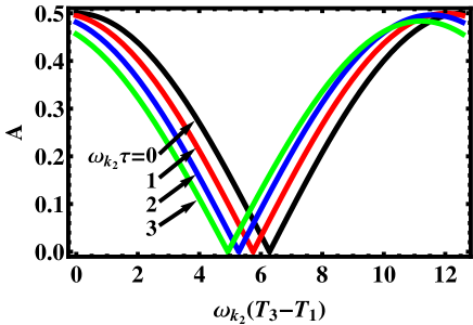
Figure 6: One period of the dependence (24) on the interrogation time $T_{3}-T_{1}$ at the optimum conditions for the different values of the recoil frequency.

One sees that outside of the Raman-Nath approximation, one can achieve almost the same magnitude of the AMZAI with the proper choice of the Raman detunings, while the interference picture shifts as a whole. The AMZAI becomes sensitive to the fields’ frequencies, but requirements for the frequencies’ stabilization are less stringent compared to the conjugate interferometers technique c14 ; c3.1 in a parameter

$$\tau/T.$$ (27)

In this article I consider only the Raman pulse beam splitter. I expect that AMZAI should also be built using a standing wave beam splitter c1 and Raman standing wave beam splitter c12 . I plan to examine these cases elsewhere.

AMZAI can be used to measure recoil frequency $\omega_{k}.$ In contrast to other interferometers used for these measurements c17 ; c20 ; c9 ; c19 ; c14 , AMZAI does not use counterpropagating effective wave vectors or standing waves. Another useful feature is that after monitoring the response as a function of the Raman field phase and measuring the difference between maximal and minimal values of the response, one gets the signal (19) insensitive to the gravity, vibration and phase noise. Calculations showed that the similar signal occurs in the interferometers c9 ; c19 ; c14 , but to our knowledge monitoring of the response for given time delay between pulses and measuring the difference between response’s maximum and minimum has never been used in those experiments. Here I propose this technique to get the signal sensitive only to the recoil frequency.

In this article a technique to obtain a signal insensitive to gravity is proposed. It was justified above only for uniform gravity. I verified that this signal can also be obtained in the presence of the gravity-gradient and Coriolis forces, if these forces are small. Only if these forces are sufficiently large, or the time delay between pulses is sufficiently long, then one can use exact expressions for the atomic trajectories (14n-14p) derived in c34 to study corresponding systematic errors in the measurement of the recoil frequency using AMZAI or technique c14 .

Supplemental Material

Appendix A MZAI with nonequal effective wave vectors

In this section, we calculate the phase of the MZAI shown in the Fig. 1 Let us consider an interaction of the atom with 3 Raman pulses having effective wave vectors $\mathbf{k}_{1}\neq\mathbf{k}_{2}\neq\mathbf{k}_{3}.$ The choice of the wave vectors $\mathbf{k}_{i}$ and times $T_{i}$ has to obey 2 constraints again. From the requirement that the blue and black lines in each port in Fig. 1 have to be parallel, i.e.

$$\mathbf{k}_{1}-2\mathbf{k}_{2}+\mathbf{k}_{3}=0,$$ (28)

The second constraint is that $D$ is the point of crossing and therefore $\overrightarrow{AB}+\overrightarrow{BD}=\overrightarrow{AC}+\overrightarrow{CD},$ which means that

$$\mathbf{k}_{1}\left(T_{2}-T_{1}\right)+\left(\mathbf{k}_{1}-\mathbf{k}_{2}\right)\left(T_{3}-T_{2}\right)=\mathbf{k}_{2}\left(T_{3}-T_{2}\right).$$ (29)

Resolving Eqs. (28, 29) in respect to the wave vectors $\mathbf{k}_{1}$ and $\mathbf{k}_{3},$ one gets

$$\mathbf{k}_{1} = 2\left(1-s\right)\mathbf{k}_{2},$$ (30a)

$$\mathbf{k}_{3} = 2s\mathbf{k}_{2},$$ (30b)

where $$s$$ is still givrn by Eq. (10). If initially an atomic density matrix is given by Eq. (12), then applying consiqently Eq. (21) from the article c8 for the density matrix evolution before and between the pulses and Eqs. (48) from the same article for the density matrix jump inside given pulse, one finds that after the 3rd pulse action, the upper state distribution is given by

$$\rho_{ee}\left(\mathbf{x},\mathbf{p},T_{3+}\right)=\rho_{b}\left(\mathbf{x},\mathbf{p}\right)+\rho_{R}\left(\mathbf{x},\mathbf{p}\right)+\rho_{i}\left(\mathbf{x},\mathbf{p}\right),$$ (31a)

$$\rho_{b}\left(\mathbf{x},\mathbf{p}\right)=\cos^{2}\left(\theta_{3}/2\right)\left\{\cos^{2}\left(\theta_{2}/2\right)\sin^{2}\left(\theta_{1}/2\right)\right.$$

$$\times f\left[\mathbf{X}\left(\mathbf{x}_{1},\mathbf{p}_{1}-\hbar\mathbf{k}_{1},-T_{1}\right),\mathbf{P}\left(\mathbf{x}_{1},\mathbf{p}_{1}-\hbar\mathbf{k}_{1},-T_{1}\right)\right]_{\left\{\mathbf{x}_{1},\mathbf{p}_{1}\right\}=\left\{\mathbf{X}\left(\mathbf{x}_{2},\mathbf{p}_{2},T_{1}-T_{2}\right),\mathbf{P}\left(\mathbf{x}_{2},\mathbf{p}_{2},T_{1}-T_{2}\right)\right\}}$$

$$+\left.\sin^{2}\left(\theta_{2}/2\right)\cos^{2}\left(\theta_{1}/2\right)f\left[\mathbf{X}\left(\mathbf{x}_{2},\mathbf{p}_{2}-\hbar\mathbf{k}_{2},-T_{2}\right),\mathbf{P}\left(\mathbf{x}_{2},\mathbf{p}_{2}-\hbar\mathbf{k}_{2},-T_{2}\right)\right]\right\}_{\left\{\mathbf{x}_{2},\mathbf{p}_{2}\right\}=\left\{\mathbf{X}\left(\mathbf{x},\mathbf{p},T_{2}-T_{3}\right),\mathbf{P}\left(\mathbf{x},\mathbf{p},T_{2}-T_{3}\right)\right\}}$$

$$+\sin^{2}\left(\theta_{3}/2\right)\left\{\sin^{2}\left(\theta_{2}/2\right)\sin^{2}\left(\theta_{1}/2\right)\right.$$

$$\times f\left[\mathbf{X}\left(\mathbf{x}_{1},\mathbf{p}_{1}-\hbar\mathbf{k}_{1},-T_{1}\right),\mathbf{P}\left(\mathbf{x}_{1},\mathbf{p}_{1}-\hbar\mathbf{k}_{1},-T_{1}\right)\right]_{\left\{\mathbf{x}_{1},\mathbf{p}_{1}\right\}=\left\{\mathbf{X}\left(\mathbf{x}_{2},\mathbf{p}_{2}+\hbar\mathbf{k}_{2},T_{1}-T_{2}\right),\mathbf{P}\left(\mathbf{x}_{2},\mathbf{p}_{2}+\hbar\mathbf{k}_{2},T_{1}-T_{2}\right)\right\}}$$

$$\left.+\cos^{2}\left(\theta_{2}/2\right)\cos^{2}\left(\theta_{1}/2\right)f\left[\mathbf{X}\left(\mathbf{x}_{2},\mathbf{p}_{2},-T_{2}\right),\mathbf{P}\left(\mathbf{x}_{2},\mathbf{p}_{2},-T_{2}\right)\right]\right\}_{\left\{\mathbf{x}_{2},\mathbf{p}_{2}\right\}=\left\{\mathbf{X}\left(\mathbf{x},\mathbf{p}-\hbar\mathbf{k}_{3},T_{2}-T_{3}\right),\mathbf{P}\left(\mathbf{x},\mathbf{p}-\hbar\mathbf{k}_{3},T_{2}-T_{3}\right)\right\}},$$ (31b)

$$\rho_{R}\left(\mathbf{x},\mathbf{p}\right)=\dfrac{1}{2}\sin\theta_{2}\sin\theta_{1}\cos\left[\mathbf{k}_{1}\cdot\mathbf{x}_{1}-\delta_{1}T_{1}-\phi_{1}-\left(\mathbf{k}_{2}\cdot\mathbf{x}_{2}-\delta_{2}T_{2}-\phi_{2}\right)\right]$$

$$\left\{\cos^{2}\left(\theta_{3}/2\right)\right.$$

$$\times\left.f\left(\begin{array}[]{c}\mathbf{X}\left(\mathbf{x}_{1},\mathbf{p}_{1}-\hbar\mathbf{k}_{1}/2,-T_{1}\right),\\ \mathbf{P}\left(\mathbf{x}_{1},\mathbf{p}_{1}-\hbar\mathbf{k}_{1}/2,-T_{1}\right)\end{array}\right)_{\left\{\mathbf{x}_{1},\mathbf{p}_{1}\right\}=\left\{\mathbf{X}\left(\mathbf{x}_{2},\mathbf{p}_{2}-\hbar\mathbf{k}_{2}/2,T_{1}-T_{2}\right),\mathbf{P}\left(\mathbf{x}_{2},\mathbf{p}_{2}-\hbar\mathbf{k}_{2}/2,T_{1}-T_{2}\right)\right\}}\right|_{\left\{\mathbf{x}_{2},\mathbf{p}_{2}\right\}=\left\{\mathbf{X}\left(\mathbf{x},\mathbf{p},T_{2}-T_{3}\right),\mathbf{P}\left(\mathbf{x},\mathbf{p},T_{2}-T_{3}\right)\right\}}$$ (31e)

$$-\sin^{2}\left(\theta_{3}/2\right)$$

$$\times\left.\left.f\left(\begin{array}[]{c}\mathbf{X}\left(\mathbf{x}_{1},\mathbf{p}_{1}-\hbar\mathbf{k}_{1}/2,-T_{1}\right),\\ \mathbf{P}\left(\mathbf{x}_{1},\mathbf{p}_{1}-\hbar\mathbf{k}_{1}/2,-T_{1}\right)\end{array}\right)_{\left\{\mathbf{x}_{1},\mathbf{p}_{1}\right\}=\left\{\begin{array}[]{c}\mathbf{X}\left(\mathbf{x}_{2},\mathbf{p}_{2}+\hbar\mathbf{k}_{2}/2,T_{1}-T_{2}\right),\\ \mathbf{P}\left(\mathbf{x}_{2},\mathbf{p}_{2}+\hbar\mathbf{k}_{2}/2,T_{1}-T_{2}\right)\end{array}\right\}}\right|_{\left\{\mathbf{x}_{2},\mathbf{p}_{2}\right\}=\left\{\mathbf{X}\left(\mathbf{x},\mathbf{p}-\hbar\mathbf{k}_{3},T_{2}-T_{3}\right),\mathbf{P}\left(\mathbf{x},\mathbf{p}-\hbar\mathbf{k}_{3},T_{2}-T_{3}\right)\right\}}\right\}$$ (31j)

$$-\dfrac{1}{2}\sin\theta_{3}\left\{\sin\theta_{2}\cos\left[\mathbf{k}_{2}\cdot\mathbf{x}_{2}-\delta_{2}T_{2}-\phi_{2}-\left(\mathbf{k}_{3}\cdot\mathbf{x}-\delta_{3}T_{3}-\phi_{3}\right)\right]\left[\sin^{2}\left(\theta_{1}/2\right)\right.\right.$$

$$\times f\left(\mathbf{X}\left(\mathbf{x}_{1},\mathbf{p}_{1}-\hbar\mathbf{k}_{1},-T_{1}\right),\mathbf{P}\left(\mathbf{x}_{1},\mathbf{p}_{1}-\hbar\mathbf{k}_{1},-T_{1}\right)\right)_{\left\{\mathbf{x}_{1},\mathbf{p}_{1}\right\}=\left\{\mathbf{X}\left(\mathbf{x}_{2},\mathbf{p}_{2}+\hbar\mathbf{k}_{2}/2,T_{1}-T_{2}\right),\mathbf{P}\left(\mathbf{x}_{2},\mathbf{p}_{2}+\hbar\mathbf{k}_{2}/2,T_{1}-T_{2}\right)\right\}}$$

$$\left.-\cos^{2}\left(\theta_{1}/2\right)f\left(\mathbf{X}\left(\mathbf{x}_{2},\mathbf{p}_{2}-\hbar\mathbf{k}_{2}/2,-T_{2}\right),\mathbf{P}\left(\mathbf{x}_{2},\mathbf{p}_{2}-\hbar\mathbf{k}_{2}/2,-T_{2}\right)\right)\right]$$

$$-\cos^{2}\left(\theta_{2}/2\right)\sin\theta_{1}\cos\left[\mathbf{k}_{1}\mathbf{x}_{1}-\delta_{1}T_{1}-\phi_{1}-\left(\mathbf{k}_{3}\mathbf{x}-\delta_{3}T_{3}-\phi_{3}\right)\right]$$

$$\times\left.f\left[\begin{array}[]{c}\mathbf{X}\left(\mathbf{x}_{1},\mathbf{p}_{1}-\hbar\mathbf{k}_{1}/2,-T_{1}\right),\\ \mathbf{P}\left(\mathbf{x}_{1},\mathbf{p}_{1}-\hbar\mathbf{k}_{1}/2,-T_{1}\right)\end{array}\right]_{\left\{\mathbf{x}_{1},\mathbf{p}_{1}\right\}=\left\{\mathbf{X}\left(\mathbf{x}_{2},\mathbf{p}_{2},T_{1}-T_{2}\right),\mathbf{P}\left(\mathbf{x}_{2},\mathbf{p}_{2},T_{1}-T_{2}\right)\right\}}\right\}_{\left\{\mathbf{x}_{2},\mathbf{p}_{2}\right\}=\left\{\mathbf{X}\left(\mathbf{x},\mathbf{p}-\hbar\mathbf{k}_{3}/2,T_{2}-T_{3}\right),\mathbf{P}\left(\mathbf{x},\mathbf{p}-\hbar\mathbf{k}_{3}/2,T_{2}-T_{3}\right)\right\}},$$ (31m)

$$\rho_{i}\left(\mathbf{x},\mathbf{p}\right)=-\dfrac{1}{2}\sin\theta_{3}\sin^{2}\left(\theta_{2}/2\right)\sin\theta_{1}\cos\left[2\left(\mathbf{k}_{2}\cdot\mathbf{x}_{2}-\delta_{2}T_{2}-\phi_{2}\right)-\left(\mathbf{k}_{1}\cdot\mathbf{x}_{1}-\delta_{1}T_{1}-\phi_{1}\right)-\left(\mathbf{k}_{3}\cdot\mathbf{x}-\delta_{3}T_{3}-\phi_{3}\right)\right]$$

$$\times\left.f\left[\begin{array}[]{c}\mathbf{X}\left(\mathbf{x}_{1},\mathbf{p}_{1}-\hbar\mathbf{k}_{1}/2,-T_{1}\right),\\ \mathbf{P}\left(\mathbf{x}_{1},\mathbf{p}_{1}-\hbar\mathbf{k}_{1}/2,-T_{1}\right)\end{array}\right]_{\left\{\mathbf{x}_{1},\mathbf{p}_{1}\right\}=\left\{\mathbf{X}\left(\mathbf{x}_{2},\mathbf{p}_{2},T_{1}-T_{2}\right),\mathbf{P}\left(\mathbf{x}_{2},\mathbf{p}_{2},T_{1}-T_{2}\right)\right\}}\right|_{\left\{\mathbf{x}_{2},\mathbf{p}_{2}\right\}=\left\{\mathbf{X}\left(\mathbf{x},\mathbf{p}-\hbar\mathbf{k}_{3}/2,T_{2}-T_{3}\right),\mathbf{P}\left(\mathbf{x},\mathbf{p}-\hbar\mathbf{k}_{3}/2,T_{2}-T_{3}\right)\right\}},$$ (31p)

where $$\theta_{i} i, \left\{\mathbf{X}\left(\mathbf{x},\mathbf{p},t\right),\mathbf{P}\left(\mathbf{x},\mathbf{p},t\right)\right\} \left\{\mathbf{x},\mathbf{p}\right\}. \left|e\right\rangle$$ is the area of the pulse are atomic classical position and momentum subject to initial value The expression (31) can be used to calculate any responce associated with atoms on the upper level. The term (31b) is caused by transfering of the atomic populations between Raman pulses first considered in c35 . This term is resposible for the background of the atomic excitation to the state .

The term (31m) is caused by transferring of the atomic coherence between two Raman pulses, saturated in the field of third Raman pulse. This term is resposible for the set of Ramsey fringes c36 . In the Doppler limitting case

$$k_{i}\dfrac{\delta p}{M}\min\left(T_{2}-T_{1},T_{3}-T_{2}\right)\gg 1,$$ (32)

where $\delta p$ is the width of the atomic momentum distribution, Ramsey fringes are washed out c37 .

The term (31p) is caused by the transfering coherence $\rho_{ge}$ between first and second pulse, mirroring it to the conerence $\rho_{eg}$ in the field of the second Raman pulse and further transfering between second and third Raman pulses. This process is responsible for the atom interference.

We use Eqs. (31) to get the probability of the excitation

$$w=\int d\mathbf{x}d\mathbf{p}\rho_{ee}\left(\mathbf{x},\mathbf{p},T_{3+}\right).$$ (33)

which consists of the backgrond and interference terms,

$$w=\bar{w}+\tilde{w}.$$ (34)

For the background term one finds from the Eq. (31b)

$$\bar{w}=1-\cos\theta_{3}\cos\theta_{2}\cos\theta_{1}.$$ (35)

To get interference term from Eq. (31p) it is convinient to use initial atomic position and momentum,

$$\left\{\mathbf{x}^{\prime},\mathbf{p}^{\prime}\right\}=\left\{\mathbf{X}\left(\mathbf{x}_{1},\mathbf{p}_{1}-\hbar\mathbf{k}_{1}/2,-T_{1}\right),\mathbf{P}\left(\mathbf{x}_{1},\mathbf{p}_{1}-\hbar\mathbf{k}_{1}/2,-T_{1}\right)\right\},$$ (36)

as the integration variables. Expressing other phase points in Eq. (31p) through the point (36) after replacement $\left\{\mathbf{x}^{\prime},\mathbf{p}^{\prime}\right\}\rightarrow\left\{\mathbf{x},\mathbf{p}\right\}$ one gets

$$\tilde{w}=-\dfrac{1}{2}\sin\theta_{3}\sin^{2}\left(\theta_{2}/2\right)\sin\theta_{1}\int d\mathbf{x}d\mathbf{p}f\left(\mathbf{x},\mathbf{p}\right)\cos\left[\phi\left(\mathbf{x},\mathbf{p}\right)-\delta_{1}T_{1}+2\delta_{2}T_{2}-\delta_{3}T_{3}-\phi_{1}+2\phi_{2}-\phi_{3}\right],$$ (37a)

$$\phi\left(\mathbf{x},\mathbf{p}\right)=\mathbf{k}_{1}\cdot\mathbf{x}_{1}-2\mathbf{k}_{2}\cdot\mathbf{x}_{2}+\mathbf{k}_{3}\cdot\mathbf{x}_{3},$$ (37b)

$$\left\{\mathbf{x}_{1},\mathbf{p}_{1}\right\}=\left\{\mathbf{X}\left(\mathbf{x},\mathbf{p},T_{1}\right),\mathbf{P}\left(\mathbf{x},\mathbf{p},T_{1}\right)+\hbar\mathbf{k}_{1}/2\right\},$$ (37c)

$$\left\{\mathbf{x}_{2},\mathbf{p}_{2}\right\}=\left\{\mathbf{X}\left(\mathbf{x}_{1},\mathbf{p}_{1},T_{2}-T_{1}\right),\mathbf{P}\left(\mathbf{x}_{1},\mathbf{p}_{1},T_{2}-T_{1}\right)\right\},$$ (37d)

$$\left\{\mathbf{x}_{3},\mathbf{p}_{3}\right\}=\left\{\mathbf{X}\left(\mathbf{x}_{2},\mathbf{p}_{2},T_{3}-T_{2}\right),\mathbf{P}\left(\mathbf{x}_{2},\mathbf{p}_{2},T_{3}-T_{2}\right)+\hbar\mathbf{k}_{3}/2\right\},$$ (37e)

where the phase of the MZAI is given by Eq. (37b). In the case of the uniform gravity field $$\mathbf{g}$$

$$\left\{\mathbf{X}\left(\mathbf{x},\mathbf{p},t\right),\mathbf{P}\left(\mathbf{x},\mathbf{p},t\right)\right\}=\left\{\mathbf{x}+\dfrac{\mathbf{p}}{M}t+\dfrac{\mathbf{g}t^{2}}{2},\mathbf{p}+M\mathbf{g}t\right\},$$ (38)

for the wave vectors (30) one arrives for the phase

$$\phi\left(\mathbf{x},\mathbf{p}\right)=s\left(1-s\right)\mathbf{k}_{2}\cdot\mathbf{g}\left(T_{3}-T_{1}\right)^{2},$$ (39)

which still contains no quantum term.

Appendix B Atomic amplitudes in the momentum state

In this appendix, we use the expressions for the atomic amplitudes’ evolution in the uniform field c11 . For the purpose of integrity we consider both the amplitudes’ evolution between Raman pulses c11 and during the interaction with a given pulse. Consider an interaction of the 3-level atom with a rectangular pulse of the 2 traveling waves

$$\mathbf{E}\left(\mathbf{x},t\right)=\left\{\mathbf{E}_{1}\exp\left[i\left(\mathbf{q}_{1}\cdot\mathbf{x}-\omega_{1}t-\phi^{\left(1\right)}\left(t\right)\right)\right]+\mathbf{E}_{2}\exp\left[i\left(\mathbf{q}_{2}\cdot\mathbf{x}-\omega_{2}t-\phi^{\left(2\right)}\left(t\right)\right)\right]\right\}f\left(t\right)+c.c.$$ (40)

where $\mathbf{E}_{i},$ $\mathbf{q}_{i},$ $\omega_{i}$ and $\phi^{\left(i\right)}\left(t\right)$ are amplitude, wave vector, frequency and phase of the waves,

$$f\left(t\right)=\left\{\begin{array}[]{c}1,\text{ for }T<t<T+\tau\\ 0,\text{ for }t<T\text{ and }t>T+\tau\end{array}\right.$$ (41)

is the shape of the rectangular pulse acting at the moment $T$ and having a duration $\tau.$ We assume that the 2 atomic states, $g$ and $e,$ are the sublevels of the atomic ground state, while the third state $0$ is an excited state, fields $\mathbf{E}_{1}$ and $\mathbf{E}_{2}$ are resonant to the transitions $g\rightarrow 0$ and $e\rightarrow 0$ correspondingly. The Hamiltonian of the atom is given by

$$H=\dfrac{\mathbf{p}^{2}}{2M}-M\mathbf{g}\cdot\mathbf{x}+\hbar\left\{\Omega^{\left(1\right)}\exp\left[i\left(\mathbf{q}_{1}\cdot\mathbf{x}-\Delta_{1}t-\phi^{\left(1\right)}\left(t\right)\right)\right]\left|0\right\rangle\left\langle g\right|+\Omega^{\left(2\right)}\exp\left[i\left(\mathbf{q}_{2}\cdot\mathbf{x}-\Delta_{2}t-\phi^{\left(2\right)}\left(t\right)\right)\right]\left|0\right\rangle\left\langle e\right|+H.c.\right\},$$ (42)

where $\Omega^{\left(1\right)}\equiv-\mathbf{d}_{0g}\cdot\mathbf{E}_{1}/\hbar$ and $\Omega^{\left(2\right)}\equiv-\mathbf{d}_{0e}\cdot\mathbf{E}_{2}/\hbar$ are Rabi frequencies, $\mathbf{d}_{0g}$ and $\mathbf{d}_{0e}$ are the matrix elements of the dipole moment operator, $\Delta_{1}=\omega_{1}-\omega_{0g}\$and $\Delta_{2}=\omega_{2}-\omega_{0e}$ are the detunings of the frequencies. Let us  eliminate an amplitude of the excited state, which evolves as

$$i\dot{a}\left(0,\mathbf{p},t\right) = \left(\dfrac{\mathbf{p}^{2}}{2M\hbar}-iM\mathbf{g}\cdot\partial_{\mathbf{p}}\right)a\left(0,\mathbf{p},t\right)$$ (43)

$$+\left\{\Omega^{\left(1\right)}e^{-i\left[\Delta_{1}t+\phi^{\left(1\right)}\left(t\right)\right]}a\left(g,\mathbf{p}-\hbar\mathbf{q}_{1},t\right)+\Omega^{\left(2\right)}e^{-i\left[\Delta_{2}t+\phi^{\left(2\right)}\left(t\right)\right]}a\left(e,\mathbf{p}-\hbar\mathbf{q}_{2},t\right)\right\}f\left(t\right).$$

When the detunings are closed

$$\Delta_{1}\approx\Delta_{2}\approx\Delta$$ (44)

and sufficiently large,

$$\left|\Delta\right|\gg Max\left\{\left|\tilde{\delta}\right|,\tau^{-1},\left|\dot{\phi}^{\left(i\right)}\right|,q_{i}gT,q_{i}\dfrac{p}{M},\omega_{q_{i}}\right\},$$ (45)

where

$$\tilde{\delta}\equiv\Delta_{1}-\Delta_{2}$$ (46)

is Raman detuning, one can neglect the first term in the right-hand-side of Eq. (43) to get

$$a\left(0,\mathbf{p},t\right)=\left\{\Omega^{\left(1\right)}\exp\left[-i\left(\Delta_{1}t+\phi^{\left(1\right)}\left(t\right)\right)\right]a\left(g,\mathbf{p}-\hbar\mathbf{q}_{1},t\right)+\Omega^{\left(2\right)}\exp\left[-i\left(\Delta_{2}t+\phi^{\left(2\right)}\left(t\right)\right)\right]a\left(e,\mathbf{p}-\hbar\mathbf{q}_{2},t\right)\right\}/\Delta,$$ (47)

where the usual assumption was accepted that the atomic ground state amplitudes vary slowly at the time $\left|\Delta\right|^{-1}.$ Substituting this expression in the equations for the atomic ground state amplitudes, one gets

$$i\left(\partial_{t}+M\mathbf{g}\cdot\partial_{\mathbf{p}}+i\dfrac{p^{2}}{2M\hbar}\right)\tilde{a}\left(e,\mathbf{p},t\right) = \dfrac{\Omega}{2}f\left(t\right)\exp\left[-i\delta t-i\phi\left(t\right)\right]\tilde{a}\left(g,\mathbf{p}-\hbar\mathbf{k},t\right),$$ (48a)

$$i\left(\partial_{t}+M\mathbf{g}\cdot\partial_{\mathbf{p}}+i\dfrac{p^{2}}{2M\hbar}\right)\tilde{a}\left(g,\mathbf{p},t\right) = \dfrac{\Omega^{\ast}}{2}f\left(t\right)\exp\left[i\delta t+i\phi\left(t\right)\right]\tilde{a}\left(e,\mathbf{p}+\hbar\mathbf{k},t\right),$$ (48b)

where $$\tilde{a}\left(g,\mathbf{p},t\right)=\exp\left(i\left|\Omega^{\left(1\right)}\right|^{2}t/\Delta\right)a\left(g,\mathbf{p},t\right);\tilde{a}\left(e,\mathbf{p},t\right)=\exp\left(i\left|\Omega^{\left(2\right)}\right|^{2}t/\Delta\right)a\left(g,\mathbf{p},t\right), \mathbf{k}=\mathbf{q}_{1}-\mathbf{q}_{2} \delta=\tilde{\delta}-\left(\left|\Omega^{\left(2\right)}\right|^{2}-\left|\Omega^{\left(1\right)}\right|^{2}\right)/\Delta, \Omega=2\Omega^{\left(1\right)}\Omega^{\left(2\right)\ast}/\Delta \phi\left(t\right)=\phi^{\left(1\right)}\left(t\right)-\phi^{\left(2\right)}\left(t\right).$$ is an effective wave vector, is Rabi Raman frequency, In the accelerated frame

$$\mathbf{p}=\mathbf{P}+M\mathbf{g}t,$$ (49)

using the initial atomic momentum $\mathbf{P}$ as an independent variable, one obtains

$$i\left(\partial_{t}+i\dfrac{\left(\mathbf{P}+M\mathbf{g}t\right)^{2}}{2M\hbar}\right)\tilde{a}\left(e,\mathbf{P},t\right) = \dfrac{\Omega}{2}f\left(t\right)\exp\left[-i\delta t-i\phi\left(t\right)\right]\tilde{a}\left(g,\mathbf{P}-\hbar\mathbf{k},t\right),$$ (50a)

$$i\left(\partial_{t}+i\dfrac{\left(\mathbf{P}+M\mathbf{g}t\right)^{2}}{2M\hbar}\right)\tilde{a}\left(g,\mathbf{P},t\right) = \dfrac{\Omega^{\ast}}{2}f\left(t\right)\exp\left[i\delta t+i\phi\left(t\right)\right]\tilde{a}\left(e,\mathbf{P}+\hbar\mathbf{k},t\right).$$ (50b)

Then one finds that in the interaction representation

$$\tilde{a}\left(n,\mathbf{P},t\right)=\exp\left[-i\int_{0}^{t}dt^{\prime}\dfrac{\left(\mathbf{P}+M\mathbf{g}t^{\prime}\right)^{2}}{2M\hbar}\right]c\left(n,\mathbf{P},t\right)$$ (51)

the vector state

$$c\left(t\right)=\left(\begin{array}[]{c}c\left(e,\mathbf{P}+\dfrac{\hbar\mathbf{k}}{2},t\right)\\ c\left(g,\mathbf{P}-\dfrac{\hbar\mathbf{k}}{2},t\right)\end{array}\right)$$ (52)

evolves as

$$i\dot{c}=\dfrac{f\left(t\right)}{2}\left(\begin{array}[]{cc}0&\Omega\exp\left\{-i\left[\delta t+\phi\left(t\right)-\mathbf{k\cdot}\dfrac{\mathbf{P}}{M}t-\dfrac{1}{2}\mathbf{k\cdot g}t^{2}\right]\right\}\\ \Omega^{\ast}\exp\left\{i\left[\delta t+\phi\left(t\right)-\mathbf{k\cdot}\dfrac{\mathbf{P}}{M}t-\dfrac{1}{2}\mathbf{k\cdot g}t^{2}\right]\right\}&0\end{array}\right)c.$$ (53)

One sees that in the accelerated frame the atomic amplitude in the interaction representation (51) stays unchanged at the pulses’ free time,

$$c\left(t\right)=\text{constant, at }t<T\text{ or }t>T+\tau.$$ (54)

If one chirps linearly the fields’ frequencies, i.e. if

$$\phi\left(t\right)=\phi+\alpha t^{2}/2$$ (55)

and if the chirping rate $\alpha$ is close to $\mathbf{k\cdot g},$

$$\left|\alpha-\mathbf{k\cdot g}\right|\tau^{2}\ll 1,$$ (56)

then one can neglect the quadratic over

$$t^{\prime}=t-T$$ (57)

terms in the phase factors in Eq. (53) and arrives at the well-known equation for the amplitudes of a two-level atom in the rectangular resonant pulse with permanent detuning and phase,

$$i\dfrac{dc}{dt^{\prime}}=\dfrac{f\left(T+t^{\prime}\right)}{2}\left(\begin{array}[]{cc}0&\Omega\exp\left\{-i\left[\delta_{\mathbf{P}}t^{\prime}+\phi\left(\mathbf{P}\right)\right]\right\}\\ \Omega^{\ast}\exp\left\{i\left[\delta_{\mathbf{P}}t^{\prime}+\phi\left(\mathbf{P}\right)\right]\right\}&0\end{array}\right)c,$$ (58)

where

$$\phi\left(\mathbf{P}\right) = \phi+\left(\delta-\mathbf{k\cdot}\dfrac{\mathbf{P}}{M}\right)T+\dfrac{1}{2}\left(\alpha-\mathbf{k\cdot g}\right)T^{2},$$ (59a)

$$\delta_{\mathbf{P}} = \partial\phi\left(\mathbf{P}\right)/\partial T.$$ (59b)

Using the solution of the Eq. (58), one finds that during an interaction with Raman pulse the atomic amplitudes jump as

$$c\left(e,\mathbf{P},T+\tau\right) = F_{ee}\left(\mathbf{P}-\hbar\mathbf{k}/2\right)c\left(e,\mathbf{P},T\right)+F_{eg}\left(\mathbf{P}-\hbar\mathbf{k}/2\right)c\left(g,\mathbf{P}-\hbar\mathbf{k},T\right),$$ (60a)

$$c\left(g,\mathbf{P},T+\tau\right) = F_{ge}\left(\mathbf{P}+\hbar\mathbf{k}/2\right)c\left(e,\mathbf{P}+\hbar\mathbf{k},T\right)+F_{gg}\left(\mathbf{P}+\hbar\mathbf{k}/2\right)c\left(g,\mathbf{P},T\right),$$ (60b)

where $$F_{m,n}\left(\mathbf{P}\right)$$ is an element of the matrix

$$F\left(\mathbf{P}\right)=\left(\begin{array}[]{cc}f_{ee}\left(\mathbf{P}\right)&f_{eg}\left(\mathbf{P}\right)\exp\left\{-i\phi\left(\mathbf{P}\right)\right\}\\ f_{ge}\left(\mathbf{P}\right)\exp\left\{i\phi\left(\mathbf{P}\right)\right\}&f_{gg}\left(\mathbf{P}\right)\end{array}\right),$$ (61)

where

$$f\left(\mathbf{P}\right) = \left(\begin{array}[]{cc}\exp\left\{-i\delta_{\mathbf{P}}\tau/2\right\}f_{d}\left[\Omega,\delta_{\mathbf{P}}\right]&-i\exp\left\{-i\delta_{\mathbf{P}}\tau/2\right\}f_{a}\left[\Omega,\delta_{\mathbf{P}}\right]\\ -i\exp\left\{i\delta_{\mathbf{P}}\tau/2\right\}f_{a}^{\ast}\left[\Omega,\delta_{\mathbf{P}}\right]&\exp\left\{i\delta_{\mathbf{P}}\tau/2\right\}f_{d}^{\ast}\left[\Omega,\delta_{\mathbf{P}}\right]\end{array}\right),$$ (62c)

$$f_{d}\left(\Omega,\delta\right) = \cos\dfrac{\Omega_{r}\left(\Omega,\delta\right)\tau}{2}+i\dfrac{\delta}{\Omega_{r}\left(\Omega,\delta\right)}\sin\dfrac{\Omega_{r}\left(\Omega,\delta\right)\tau}{2},$$ (62d)

$$f_{a}\left(\Omega,\delta\right) = \dfrac{\Omega}{\Omega_{r}\left(\Omega,\delta\right)}\sin\dfrac{\Omega_{r}\left(\Omega,\delta\right)\tau}{2},$$ (62e)

$$\Omega_{r}\left(\Omega,\delta\right) = \sqrt{\left|\Omega\right|^{2}+\delta^{2}}.$$ (62f)

Appendix C AMZAI response

Let us now apply Eqs. (54, 60) to consider AMZAI, i.e. to calculate the total probability of the atoms’ excitation

$$w=\int d\mathbf{P}\left|c\left(e,\mathbf{P},T_{3}+\tau\right)\right|^{2}$$ (63)

with 3 Raman pulses and one microwave pulse having Rabi frequencies $\left\{\Omega_{1},\Omega_{2},\Omega_{m},\Omega_{3}\right\},$ detunings $\left\{\delta_{1},\delta_{2},\delta_{m},\delta_{3}\right\},$ phases $\left\{\phi_{1},\phi_{2},\phi_{m},\phi_{3}\right\},$ wave vectors and chirping rates

$$\left\{\mathbf{k}_{1},\mathbf{k}_{2},\mathbf{k}_{m},\mathbf{k}_{3}\right\} = \mathbf{k}_{2}\left\{1-s,1,0,s\right\},$$ (64a)

$$\left\{\alpha_{1},\alpha_{2},\alpha_{m},\alpha_{3}\right\} = \alpha_{2}\left\{1-s,1,0,s\right\},$$ (64b)

and acting at the moments $$\left\{T_{1},T_{2},T_{m},T_{3}\right\}. \left[c\left(e,\mathbf{P},T_{1}\right)=0\right],$$ Assuming that before the pulses action atoms are in the ground state only and using consequently the Eqs. (60) for each pulse one arrives to the following result

$$c\left(e,\mathbf{P},T_{3}+\tau\right) = c_{1+}+c_{2+}+c_{1-}+c_{2-}$$ (65)

$$+F_{3ee}\left(\mathbf{P}-s\hbar\mathbf{k}_{2}/2\right)\left[F_{mee}F_{2ee}\left(\mathbf{P}-\hbar\mathbf{k}_{2}/2\right)F_{1eg}\left(\mathbf{P}-\left(1-s\right)\hbar\mathbf{k}_{2}/2\right)c\left(g,\mathbf{P}-\left(1-s\right)\hbar\mathbf{k}_{2},T_{1}\right)\right.$$

$$\left.+F_{meg}F_{2ge}\left(\mathbf{P}+\hbar\mathbf{k}_{2}/2\right)F_{1eg}\left(\mathbf{P}+\left(1+s\right)\hbar\mathbf{k}_{2}/2\right)c\left(g,\mathbf{P}+s\hbar\mathbf{k}_{2},T_{1}\right)\right]$$

$$+F_{3eg}\left(\mathbf{P}-s\hbar\mathbf{k}_{2}/2\right)\left[F_{mge}F_{2eg}\left(\mathbf{P}-\left(2s+1\right)\hbar\mathbf{k}_{2}/2\right)F_{1gg}\left(\mathbf{P}-\left(3s+1\right)\hbar\mathbf{k}_{2}/2\right)c\left(g,\mathbf{P}-\left(s+1\right)\hbar\mathbf{k}_{2},T_{1}\right)\right.$$

$$+\left.F_{mgg}F_{2gg}\left(\mathbf{P}-\left(2s-1\right)\hbar\mathbf{k}_{2}/2\right)F_{1gg}\left(\mathbf{P}-\left(3s-1\right)\hbar\mathbf{k}_{2}/2\right)c\left(g,\mathbf{P}-s\hbar\mathbf{k}_{2},T_{1}\right)\right],$$

where

$$c_{1+} = F_{3ee}\left(\mathbf{P}-s\hbar\mathbf{k}_{2}/2\right)F_{mee}F_{2eg}\left(\mathbf{P}-\hbar\mathbf{k}_{2}/2\right)F_{1gg}\left(\mathbf{P}-\left(1+s\right)\hbar\mathbf{k}_{2}/2\right)c\left(g,\mathbf{P}-\hbar\mathbf{k}_{2},T_{1}\right),$$ (66a)

$$c_{2+} = F_{3eg}\left(\mathbf{P}-s\hbar\mathbf{k}_{2}/2\right)F_{mge}F_{2ee}\left(\mathbf{P}-\left(2s+1\right)\hbar\mathbf{k}_{2}/2\right)F_{1eg}\left(\mathbf{P}-\left(1+s\right)\hbar\mathbf{k}_{2}/2\right)c\left(g,\mathbf{P}-\hbar\mathbf{k}_{2},T_{1}\right),$$ (66b)

$$c_{1-} = F_{3ee}\left(\mathbf{P}-s\hbar\mathbf{k}_{2}/2\right)F_{meg}F_{2gg}\left(\mathbf{P}+\hbar\mathbf{k}_{2}/2\right)F_{1gg}\left(\mathbf{P}+\left(1-s\right)\hbar\mathbf{k}_{2}/2\right)c\left(g,\mathbf{P},T_{1}\right),$$ (66c)

$$c_{2-} = F_{3eg}\left(\mathbf{P}-s\hbar\mathbf{k}_{2}/2\right)F_{mgg}F_{2ge}\left(\mathbf{P}-\left(2s-1\right)\hbar\mathbf{k}_{2}/2\right)F_{1eg}\left(\mathbf{P}+\left(1-s\right)\hbar\mathbf{k}_{2}/2\right)c\left(g,\mathbf{P},T_{1}\right),$$ (66d)

$$F_{N\alpha\beta} \left(\alpha\beta\right)- N. \bar{w} \left|c\left(g,\mathbf{P},T_{1}\right)\right|^{2} \mathbf{P}_{0}$$ is element of matrix (61) associated with the pulse The sum of the 8 integrals of the absolute squares of the each term in (65) is a background of the response (63), while the cross terms are responsible for the interference. If the initial atomic distribution is centered near the momentum and, after using the filtering technique c10 ; c33 , it is narrowed to the width

$$\delta P\ll\dfrac{M}{k\tau}$$ (67)

and if the pulse duration is comparable to the inverse recoil frequency, then different terms in Eq. (65) are centered in the momentum space near the points which are far distanced from one another and cannot interfere. There are only 2 exclusions, 2 pairs of the terms $\left\{c_{1+,}c_{2+}\right\},$ located at the point $\mathbf{P}=\mathbf{P}_{0}+\hbar\mathbf{k}_{2},$ and $\left\{c_{1-,}c_{2-}\right\},$ located at the point $\mathbf{P}=\mathbf{P}_{0},$ leading to the interferometric part of the excitation probability

$$\tilde{w} = w_{+}+w_{-},$$ (68a)

$$w_{\pm} = 2\mathop{\mathrm{R}e}\int d\mathbf{P}c_{1\pm}c_{2\pm}^{\ast}$$ (68b)

For the parameter $$s \thicksim M/k_{2}T f_{N}\left(\mathbf{P}\right), \thicksim M/k\tau, c\left(g,\mathbf{P},T_{1}\right)=\sqrt{\delta\left(\mathbf{P}-\mathbf{P}_{0}\right)}$$ given by Eq. (10) the rapid oscillations of the integrands in Eq. (68b) as functions of the momentum with period disappear. Other factors originated from the matrices given by Eq. (62c), are smooth functions of the momentum with size so that one can put in Eqs. (66) to find

$$w_{\pm} = -2\mathop{\mathrm{R}e}\left\{\exp\left[i\left(-\phi_{I}-\phi_{c}+\left(-\delta_{m}+\delta_{1,\mathbf{P}_{0}}-\omega_{k_{2}}\left(1-s\right)^{2}\right)\tau\right)\mp r\right]xx_{\pm}\right\},$$ (69a)

$$r = \phi_{q}-s\omega_{k_{2}}\tau;$$ (69b)

$$\phi_{c} = \dfrac{1}{2}\left(\mathbf{k}_{2}\cdot\mathbf{g}-\alpha_{2}\right)s\left(1-s\right)\left(T_{3}-T_{1}\right)^{2},$$ (69c)

$$x = f_{d}^{\ast}\left[\Omega_{1},\delta_{1,\mathbf{P}_{0}}-\left(1-s\right)^{2}\omega_{k_{2}}\right]f_{a}\left[\left|\Omega_{1}\right|,\delta_{1,\mathbf{P}_{0}}-\left(1-s\right)^{2}\omega_{k_{2}}\right]f_{a}\left[\left|\Omega_{m}\right|,\delta_{m}\right]f_{d}\left[\Omega_{m},\delta_{m}\right],$$ (69d)

$$x_{+} = f_{d}\left[\Omega_{3},\delta_{3,\mathbf{P}_{0}}-s\left(2-s\right)\omega_{k_{2}}\right]f_{a}\left[\left|\Omega_{3}\right|,\delta_{3,\mathbf{P}_{0}}-s\left(2-s\right)\omega_{k_{2}}\right]$$ (69e)

$$\times f_{a}\left[\left|\Omega_{2}\right|,\delta_{2,\mathbf{P}_{0}}-\omega_{k_{2}}\right]f_{d}^{\ast}\left[\Omega_{2},\delta_{2,\mathbf{P}_{0}}-\left(1-2s\right)\omega_{k_{2}}\right],$$

$$x_{-} = f_{d}\left[\Omega_{3},\delta_{3,\mathbf{P}_{0}}+s^{2}\omega_{k_{2}}\right]f_{a}\left[\left|\Omega_{3}\right|,\delta_{3,\mathbf{P}_{0}}+s^{2}\omega_{k_{2}}\right]$$ (69f)

$$\times f_{d}^{\ast}\left[\Omega_{2},\delta_{2,\mathbf{P}_{0}}-\omega_{k_{2}}\right]f_{a}\left[\left|\Omega_{2}\right|,\delta_{2,\mathbf{P}_{0}}+\left(2s-1\right)\omega_{k_{2}}\right],$$

where the quantum phase $$\phi_{q} \phi_{I} \phi_{c}.$$ and phase are given by Eqs.(17c, 14h), and Eq. (69c) now defines the classical phase

Calculating the absolute squares of the terms in Eq, (65), one arrives at the following results for the background term

$$\bar{w} = \left|f_{a}\left[\Omega_{1},\delta_{1,\mathbf{P}_{0}}-\left(1-s\right)^{2}\omega_{k_{2}}\right]\right|^{2}\left\{\left|f_{d}\left[\Omega_{m},\delta_{m}\right]\right|^{2}\left[\left|f_{d}\left(\Omega_{3},\delta_{3,\mathbf{P}_{0}}-s\left(2-s\right)\omega_{k_{2}}\right)f_{d}\left(\Omega_{2},\delta_{2,\mathbf{P}_{0}}-\left(1-2s\right)\omega_{k_{2}}\right)\right|^{2}\right.\right.$$ (70)

$$\left.+\left|f_{a}\left(\Omega_{3},\delta_{3,\mathbf{P}_{0}}+s^{2}\omega_{k_{2}}\right)f_{a}\left(\Omega_{2},\delta_{2,\mathbf{P}_{0}}-\left(1-2s\right)\omega_{k_{2}}\right)\right|^{2}\right]$$

$$+\left|f_{a}\left[\Omega_{m},\delta_{m}\right]\right|^{2}\left[\left|f_{d}\left(\Omega_{3},\delta_{3,\mathbf{P}_{0}}+3s^{2}\omega_{k_{2}}\right)f_{a}\left(\Omega_{2},\delta_{2,\mathbf{P}_{0}}-\left(1-2s\right)\omega_{k_{2}}\right)\right|^{2}\right.$$

$$\left.\left.+\left|f_{a}\left(\Omega_{3},\delta_{3,\mathbf{P}_{0}}-s\left(2-s\right)\omega_{k_{2}}\right)f_{d}\left(\Omega_{2},\delta_{2,\mathbf{P}_{0}}-\left(1-2s\right)\omega_{k_{2}}\right)\right|^{2}\right]\right\}$$

$$+\left|f_{d}\left[\Omega_{1},\delta_{1,\mathbf{P}_{0}}-\left(1-s\right)^{2}\omega_{k_{2}}\right]\right|^{2}\left\{\left|f_{d}\left[\Omega_{m},\delta_{m}\right]\right|^{2}\left[\left|f_{d}\left(\Omega_{3},\delta_{3,\mathbf{P}_{0}}-s\left(2-s\right)\omega_{k_{2}}\right)f_{a}\left(\Omega_{2},\delta_{2,\mathbf{P}_{0}}-\omega_{k_{2}}\right)\right|^{2}\right.\right.$$

$$+\left.\left|f_{a}\left(\Omega_{3},\delta_{3,\mathbf{P}_{0}}-s^{2}\omega_{k_{2}}\right)f_{d}\left(\Omega_{2},\delta_{2,\mathbf{P}_{0}}-\omega_{k_{2}}\right)\right|^{2}\right]$$

$$+\left|f_{a}\left[\Omega_{m},\delta_{m}\right]\right|^{2}\left[\left|f_{d}\left(\Omega_{3},\delta_{3,\mathbf{P}_{0}}+s^{2}\omega_{k_{2}}\right)f_{d}\left(\Omega_{2},\delta_{2,\mathbf{P}_{0}}-\omega_{k_{2}}\right)\right|^{2}\right.$$

$$\left.\left.+\left|f_{a}\left(\Omega_{3},\delta_{3,\mathbf{P}_{0}}-s\left(2+s\right)\omega_{k_{2}}\right)f_{a}\left(\Omega_{2},\delta_{2,\mathbf{P}_{0}}-\omega_{k_{2}}\right)\right|^{2}\right]\right\}.$$

References

• (1) B. Dubetsky, A. P. Kazantsev, V. P. Chebotayev, V. P. Yakovlev, Pis’ma Zh. Eksp. Teor. Fiz. 39, 531 (1984) [JETP Lett. 39, 649 (1984)].
• (2) Ye. V. Baklanov, B. Dubetsky, V. M. Semibalamut, Zh. Eksp. Teor. Fiz. 76, 482 (1979) [JETP 49, 244 (1979)].
• (3) V. P. Chebotayev, B. Dubetsky, A. P. Kazantsev, V. P. Yakovlev, J. Opt. Soc. Am. B 2, 1791 (1985).
• (4) S. B. Cahn, A. Kumarakrishnan, U. Shim, T. Sleator, P. R. Berman, B. Dubetsky, Phys. Rev. Lett. 79, 784 (1997).
• (5) M. S. Chapman, C. R. Ekstrom, T. D. Hammond, J. Schmiedmayer, B. E. Tannian, S. Wehinger, D. E. Pritchard, Phys. Rev. A 51, R14 (1995).
• (6) D. S. Weiss, B. C. Young, S. Chu, Phys. Rev. Lett., 70, 2706 (1993).
• (7) Ch. J. Borde, Phys. Lett. 140, 10 (1989).
• (8) B. Estey, C. Yu, and H. MΓΌller, Phys. Rev. Lett. 115, 083002 (2015).
• (9) Expression (5) for the phase has been first derived for neutron interferometer, see Eq. (4.8) in D. M. Greenberger, A. W. Overhauser, Rev. Mod. Phys.Β 51, 43 (1979).
• (10) B. Dubetsky, S. B. Libby and P. Berman, Atoms 4, 14 (2016).
• (11) M. Kasevich, S. Chu, Phys. Rev. Lett., 67, 181 (1991).
• (12) B. Dubetsky and P. R. Berman, Phys. Rev. A 56, R1091 (1997).
• (13) K. Bongs, R. Launay, and M. A. Kasevich, Appl. Phys. B 84, 599 (2006).
• (14) B. Dubetsky, M. A. Kasevich, Phys. Rev. A 74, 023615 (2006).
• (15) P. Asenbaum, C. Overstreet, T. Kovachy, D. D. Brown, J. M. Hogan, and M. A. Kasevich, Phys. Rev. Lett. 118, 183602 (2017).
• (16) S.-w. Chiow, S. Herrmann, S. Chu,and H. MΓΌller, Phys. Rev. Lett. 103, 050402 (2009).
• (17) M. A. Kasevich, Private comunication (2017)
• (18) T. Sleator, T. Pfau, V. Balykin, J. Mlynek, Appl. Phys. B 54, 375 (1992).
• (19) B. Dubetsky and P. R. Berman, Phys. Rev. A 58, 2413 (1998).
• (20) J. L. Cohen, B. Dubetsky, and P. R. Berman, Phys. Rev. A 60, 3982 (1999).
• (21) T. Kovachy, P. Asenbaum, C. Overstreet, C. A. Donnelly, S. M. Dickerson, A. Sugarbaker, J. M. Hogan & M. A. Kasevich, Nature 528, 530 (2015).
• (22) A. Roura, Phys. Rev. Lett. 118,160401 (2017).
• (23) C. Overstreet, P. Asenbaum, T. Kovachy, R. Notermans, J. M. Hogan, M. A. Kasevich, https://arxiv.org/abs/1711.09986.
• (24) G. D’Amico, G. Rosi, S. Zhan, L. Cacciapuoti, M. Fattori, and G. M. Tino, Phys. Rev. Lett. 119, 253201 (2017).
• (25) B. Dubetsky, G. Raithel, http://arxiv.org/abs/physics/0206029.
• (26) One can expect that a necessity of the microwave pulse disappears if one uses the standing wave beam splitter c1 in the Raman-Nath or Bragg regime, which does not change the internal state of the atom.
• (27) C. Mok, B. Barrett, A. Carew, R. Berthiaume, S. Beattie, and A. Kumarakrishnan, Phys. Rev. A 88, 023614 (2013).
• (28) B. Barrett, L. Antoni-Micollier, L. Chichet, B. Battelier, P.-A.Gominet, A. Bertoldi, P. Bouyer, A. Landragin, New J. Phys. 17, 085010 (2015).
• (29) X. Zhang, R. P. del Aguila, T. Mazzoni, N. Poli, and G. M. Tino, Phys. Rev. A 94, 043608 (2016).
• (30) B. Barrett1, L. Antoni-Micollier1, L. Chichet, B. Battelier, T. LΓ©vΓ¨que, A. Landragin & P. Bouyer, Nat. Commun. 7, 13786 (2016).
• (31) J. M. Hogan, D. M. S. Johnson, M. A. Kasevich, https://arxiv.org/abs/0806.3261.
• (32) T. Farah, P. Gillot, B. Cheng, A. Landragin, S. Merlet, and F. Pereira Dos Santos, Phys. Rev. A 90, 023606 (2014).
• (33) G. D’Amico, F. Borselli, L. Cacciapuoti, M. Prevedelli, G. Rosi, F. Sorrentino, and G. M. Tino, Phys. Rev. A 93, 063628 (2016).
• (34) J. K. Stockton, K. Takase, and M. A. Kasevich, Phys. Rev. Lett. 107, 133001 (2011).
• (35) M. Meunier, I. Dutta, R. Geiger,Β C. Guerlin,Β C. L. Garrido Alzar, and A. Landragin, Phys. Rev. A 90, 063633 (2014).
• (36) G. Rosi, G. D’Amico, L. Cacciapuoti, F. Sorrentino, M. Prevedelli, M. Zych, C. Brukner, G. M. Tino, Nat. Commun.Β 8, 15529 (2017).
• (37) J. M. McGuirk, M. J. Snadden, and M. A. Kasevich, Phys. Rev. Lett. 85, 4498 (2000).
• (38) S. M. Dickerson, J. M. Hogan, A. Sugarbaker, D. M. S. Johnson, and M. A. Kasevich, Phys. Rev. Lett. 111, 083001 (2013).
• (39) B. Dubetsky and P. R. Berman, Laser Physics, 12, 1161 (2002), the Raman standing wave scheme is also known as double-diffraction technique c13 .
• (40) T. LΓ©vΓ¨que, A. Gauguet, F. Michaud, F. Pereira Dos Santos, A. Landragin, Phys. Rev. Lett. 103, 080405 (2009).
• (41) M. A. Kasevich and B. Dubetsky, U.S. Patent 7,317,184, 8 January 2008.
• (42) V. S. Letokhov, B. D. Pavlik, Optika i Spektosk. 32, 856 (1972) [Opt. Spectrosc. 32, 456 (1972)].
• (43) N. F. Ramsey, Phys. Rev. 76, 996 (1949).
• (44) A. N. Oraevsky,, IEEE Trans. IM-17, 346 (1968)