Hyperfield Grassmannians

Abstract

In a recent paper Baker and Bowler introduced matroids over hyperfields, offering a common generalization of matroids, oriented matroids, and linear subspaces of based vector spaces. This paper introduces the notion of a topological hyperfield and explores the generalization of Grassmannians and realization spaces to this context, particularly in relating the (hyper)fields $\mathbb{R}$ and $\mathbb{C}$ to hyperfields arising in matroid theory and in tropical geometry.

1 Introduction

In a recent paper [BB16] Baker and Bowler introduced matroids over hyperfields, a compelling unifying theory that spans, among other things,

1. matroid theory,

2. subspaces of based vector spaces, and

3. “tropical” analogs to subspaces of vector spaces.

A hyperfield is similar to a field, except that addition is multivalued. Such structures may seem exotic, but, for instance, Viro has argued persuasively [Vir10], [Vir11] for their naturalness in tropical geometry, and Baker and Bowler’s paper elegantly demonstrates how matroids and related objects (e.g. oriented matroids, valuated matroids) can be viewed as “subspaces of $F^{n}$, where $F$ is a hyperfield”. Baker and Bowler’s work on hyperfields was purely algebraic and combinatorial; no topology was introduced.

The purpose of this paper is to explore topological aspects of matroids over hyperfields, specifically Grassmannians over hyperfields and realization spaces of matroids over hyperfields. The idea of introducing a topology on a hyperfield is problematic from the start: as Viro discusses in [Vir10], there are complications even in defining the notion of a continuous multivalued function, for example, hyperfield addition. That being said, we define a notion of a topological hyperfield that suffices to induce topologies on the related Grassmannians and sets of realizations, so that continuous homomorphisms between topological hyperfields induce continuous maps between related spaces such as Grassmannians.

We focus on Diagram (1) of hyperfield morphisms (which are all continuous with respect to appropriate topologies), categorical considerations, and the induced realization spaces and maps of Grassmannians. Most of this collection of hyperfields was discussed at length in [Vir10] and [Vir11]. Loosely put, most of the top half of the diagram describes the fields $\mathbb{R}$ and $\mathbb{C}$ and their relationship to oriented matroids, phased matroids, and matroids – relationships which have been extensively studied and are known to be fraught. The bottom half of the diagram is in some sense a tropical version of the top half. In particular, the hyperfield $\mathcal{T}\triangle$ in the bottom row is isomorphic to the “tropical hyperfield”, which is called $\mathbb{Y}$ in [Vir10] and captures the $(\max,+)$ arithmetic of the tropical semifield [BS14]. The hyperfield $\mathcal{T}\mathbb{C}$ in the bottom row has not been widely studied, but, as Viro [Vir10] notes, algebraic geometry over this hyperfield “occupies an intermediate position between the complex algebraic geometry and tropical geometry”. Each of the hyperfields in the bottom row arises from the corresponding hyperfield in the first row by “dequantization”, a process introduced and discussed in detail in [Vir10] and reviewed briefly in Section 2.2. The maps going upwards in the bottom half of the diagram are quotient maps in exactly the same way as the corresponding maps going downwards in the top half.

With Diagrams (1) and (2) we lay out a framework for relating several spaces (Grassmannians and realization spaces) and continuous maps between them, and with Theorems 4.4 and 5.6 we show some of these spaces to be contractible and some of these maps to be homotopy equivalences. We find some striking differences between the top half and bottom half of the diagram. For instance, it is well known that realization spaces of oriented matroids over $\mathbb{R}$ can have very complicated topology, and can even be empty. In our framework, such spaces arise from the hyperfield morphism $\mathbb{R}\to\mathbb{S}$. In contrast, realization spaces of oriented matroids over the topological “tropical real” hyperfield $\mathcal{T}\mathbb{R}$, which arise from the hyperfield morphism $\mathcal{T}\mathbb{R}\to\mathbb{S}$, are all contractible.

Our enthusiasm for topological hyperfields arose from the prospect of recasting our previous work [AD02] on combinatorial Grassmannians in terms of Grassmannians over hyperfields. Motivated by a program of MacPherson [Mac93], we defined a notion of a matroid bundle based on oriented matroids, described the process of proceeding from a vector bundle to a matroid bundle, defined a map of classifying spaces ${\widetilde{\mu}}:\operatorname{Gr}(r,\mathbb{R}^{n})\to\|\mathrm{MacP}(r,n)\|$, and showed that, stably, ${\widetilde{\mu}}$ induces a split surjection in mod 2 cohomology. Here $\mathrm{MacP}(r,n)$ is the finite poset of rank $r$ oriented matroids on $n$ elements and $\|\mathrm{MacP}(r,n)\|$ is its geometric realization. One of the topological hyperfields we consider in the current paper is the sign hyperfield $\mathbb{S}$. The poset $\mathrm{MacP}(r,n)$ coincides as a set with the Grassmannian $\operatorname{Gr}(r,\mathbb{S}^{n})$. We will relate the partial order on $\mathrm{MacP}(r,n)$ to the topology on $\operatorname{Gr}(r,\mathbb{S}^{n})$ to see that $\|\mathrm{MacP}(r,n)\|$ and $\operatorname{Gr}(r,\mathbb{S}^{n})$ have the same weak homotopy type, and hence the same cohomology. Further, the Grassmannian $\operatorname{Gr}(r,\mathcal{T}\mathbb{R}_{0}^{n})$ over the tropical real hyperfield is homotopy equivalent to $\operatorname{Gr}(r,\mathbb{S}^{n})$. Summarizing,

Theorem 1.1.

1. There is a weak homotopy equivalence $\|\mathrm{MacP}(r,n)\|\to\operatorname{Gr}(r,\mathbb{S}^{n})$.

2. There are maps of topological hyperfields

   $$\mathbb{R}\to\mathbb{S}\to\mathcal{T}\mathbb{R}_{0}$$

   inducing continuous maps $\operatorname{Gr}(r,\mathbb{R}^{n})\to\operatorname{Gr}(r,\mathbb{S}^{n})\to\operatorname{Gr}(r,\mathcal{T}\mathbb{R}_{0}^{n})$. The first Grassmannian map gives a surjection in mod 2 cohomology and the second is a homotopy equivalence.

The Grassmannians $\operatorname{Gr}(r,\mathbb{R}^{n})$ and $\operatorname{Gr}(r,\mathbb{C}^{n})$ are already well understood and, indeed, of central importance in topology. The Grassmannian $\operatorname{Gr}(r,\mathbb{S}^{n})=\mathrm{MacP}(r,n)\simeq\operatorname{Gr}(r,\mathcal{T}\mathbb{R}_{0}^{n})$ is a space which has been studied but remains somewhat mysterious: its topology is discussed in Section 7. The Grassmannian $\operatorname{Gr}(r,\mathbb{K}^{n})$ is contractible. Beyond what is presented in this paper, the remaining spaces appear to be considerably more difficult to understand. We hope that the discussion here stimulates interest in pursuing the topology of these spaces. To repeat a remark we made previously on the MacPhersonian [AD02]: “there are open questions everywhere you spit”.

2 Hyperfields

Much of the following is background material taken from [Vir10] and [BB16].

2.1 Examples

This section owes much to the paper of Oleg Viro [Vir10].

A hyperoperation on a set $S$ is a function from $S\times S$ to the set of nonempty subsets of $S$. A abelian hypergroup $(S,\boxplus,0)$ is a set $S$, a hyperoperation $\boxplus$ on $S$, and an element $0\in S$ satisfying

• For all $x,y\in S$, $x\boxplus y=y\boxplus x$.

• For all $x,y,z\in S$, $(x\boxplus y)\boxplus z=x\boxplus(y\boxplus z)$.

• For all $x\in S$, $x\boxplus 0=x$.

• For all $x\in S$, there is a unique $-x\in S$ such that $0\in x\boxplus-x$.

• For all $x,y,z\in S$, $x\in y\boxplus z\Leftrightarrow-x\in-y\boxplus-z$.

Here we define hyperoperations applied to sets in the obvious way. For instance, $(x\boxplus y)\boxplus z$ is the union of $u\boxplus z$ over all $u\in x\boxplus y$.

The last axiom for an abelian hypergroup $S$ can be replaced by:

• Reversibility: For all $x,y,z\in S$, $x\in y\boxplus z\Leftrightarrow z\in x\boxplus-y$.

In the literature, an abelian hypergroup as above is sometimes called a canonical hypergroup.

A hyperfield is a tuple $(F,\odot,\boxplus,1,0)$ consisting of a set, an operation, a hyperoperation, and two special elements $1\neq 0$ such that

• $(F,\boxplus,0)$ is an abelian hypergroup.

• $(F-\{0\},\odot,1)$ is a abelian group, denoted by $F^{\times}$.

• For all $x\in F$, $0\odot x=0=x\odot 0$.

• $x\odot(y\boxplus z)=(x\odot y)\boxplus(x\odot z)$.

We will often abbreviate and say that $F$ is a hyperfield.

The following property may or may not hold for a hyperfield $F$:

• Doubly distributive property: For all $w,x,y,z\in F$, $(w\boxplus x)\odot(y\boxplus z)=(w\odot y)\boxplus(w\odot z)\boxplus(x\odot y)\boxplus(x\odot z)$

Suppose $K$ is a field. Here are two constructions of associated hyperfields:

• Suppose $S$ be a subgroup of the multiplicative group of units $K^{\times}$. Then $K/_{m}S:=\{0\}\cup K^{\times}/S$ is a hyperfield with $[a]\odot[b]=[ab]$ and $[a]\boxplus[b]=\{[c]:c\in[a]+[b]\}$. Here $[0]=0\in K/_{m}S$ and for $a\in K^{\times}$, $[a]=aS$. Note that $[a]\boxplus[b]$ is independent of the choice of representatives for $[a]$ and $[b]$.

  More generally, let $(F,\odot,\boxplus,1,0)$ be a hyperfield and $S$ be a subgroup of the multiplicative group of units $F^{\times}=F-\{0\}$. Then $F/_{m}S=\{0\}\cup F^{\times}/S$ is a hyperfield with $[a]\odot[b]=[a\odot b]$ and $[a]\boxplus[b]=\{[c]:c\in[a]\boxplus[b]\}$.

• Suppose $K=K_{-}\cup\{0\}\cup K_{+}$ is an ordered field. Define a hyperfield $F$ with $F^{\times}=K^{\times}$, but with

  $$a\boxplus b=\begin{cases}a&\text{if }|a|>|b|\\ a&\text{if }a=b\\ [-|a|,|a|]&\text{if }a=-b\end{cases}$$

A homomorphism of hyperfields is a function $h:F\to F^{\prime}$ such that $h(0)=0$, $h(1)=1$, $h(x\odot y)=h(x)\odot h(y)$ and $h(x\boxplus y)\subseteq h(x)\boxplus h(y)$.

Many examples of hyperfields and homomorphisms are encoded in the diagram below.

(1)

The diagram with the solid arrows commutes. The four dashed arrows are inclusions giving sections (one-sided inverses). Here $\operatorname{ph}$ is the phase map $\operatorname{ph}(x)=x/|x|$ if $x\neq 0$ and $\operatorname{ph}(0)=0$.

In each of the ten hyperfields, the underlying set is a subset of the complex numbers closed under multiplication. And, in each hyperfield, multiplication, the additive identity, and the multiplicative identity coincides with that of the complex numbers.

Here are the hyperfields in the diagram:

1. $\mathbb{R}$ is the field of real numbers. $\mathbb{C}$ is the field of complex numbers.

2. $\triangle=(\mathbb{R}_{\geq 0},\times,\boxplus,1,0)$ is the triangle hyperfield of Viro [Vir10]. Here $a\boxplus b=\{c:|a-b|\leq c\leq a+b\}$ which can be interpreted as the set of all numbers $c$ such that there is a triangle with sides of length $a,b,c$. Note that the additive inverse of $a$ is $a$.

3. $\mathbb{P}=(S^{1}\cup\{0\},\times,\boxplus,1,0)$ is the phase hyperfield. If $a\in S^{1}$, then $a\boxplus-a=\{-a,0,a\}$ and $a\boxplus a=a$. If $a,b\in S^{1}$ and $a\neq\pm b$, then $a\boxplus b$ is the shortest open arc connecting $a$ and $b$. Note that the additive inverse of $a$ is $-a$.

4. $\mathbb{S}=(\{-1,0,1\},\times,\boxplus,1,0)$ is the sign hyperfield. Here $1\boxplus 1=1$, $-1\boxplus-1=-1$, and $1\boxplus-1=\{-1,0,1\}$. Note that the additive inverse of $a$ is $-a$.

5. $\Phi=(S^{1}\cup\{0\},\times,\boxplus,1,0)$ is the tropical phase hyperfield. If $a\in S^{1}$, then $a\boxplus-a=S^{1}\cup\{0\}$ and $a\boxplus a=a$. If $a,b\in S^{1}$ and $a\neq\pm b$, then $a\boxplus b$ is the shortest closed arc connecting $a$ and $b$. Note that the additive inverse of $a$ is $-a$.

6. $\mathbb{K}=(\{0,1\},\times,\boxplus,1,0)$ is the Krasner hyperfield. Here $1\boxplus 1=\{0,1\}$. Note that the additive inverse of $a$ is $a$.

7. ${\mathcal{T}}\mathbb{R}=(\mathbb{R},\times,\boxplus,1,0)$ is the tropical real hyperfield. Here if $|a|>|b|$, then $a\boxplus b=a$. Also $a\boxplus a=a$ and $a\boxplus-a=[-|a|,|a|]$. Note that the additive inverse of $a$ is $-a$. This hyperfield was studied by Connes and Consani [CC15], motivated by considerations in algebraic arithmetic geometry.

8. ${\mathcal{T}}\mathbb{C}=(\mathbb{C},\times,\boxplus,1,0)$ is the tropical complex hyperfield. One defines $a\boxplus-a=\{x\in\mathbb{C}:|x|\leq|a|\}$, the disk of radius $|a|$ about the origin. If $|a|>|b|$, then $a\boxplus b=a$. If $|a|=|b|$ and $a\neq-b$, then $a\boxplus b$ is the shortest closed arc connecting $a$ and $b$ on the circle of radius $|a|$ with center the origin. Note that the additive inverse of $a$ is $-a$.

9. ${\mathcal{T}}\triangle=(\mathbb{R}_{\geq 0},\times,\boxplus,1,0)$ is the tropical triangle hyperfield. Here if $a>b$, then $a\boxplus b=a$, and $a\boxplus a=[0,a]$. Note that the additive inverse of $a$ is $a$.

   The logarithm map from $\mathcal{T}\triangle$ to $\mathbb{R}\cup\{-\infty\}$ induces a hyperfield structure on $\mathbb{R}\cup\{-\infty\}$. Following [Vir10] we denote this hyperfield $\mathbb{Y}$ and call it the tropical hyperfield. In tropical geometry it is standard to work with the tropical semifield, whose only difference from $\mathbb{Y}$ is that $a\boxplus b$ is defined to be $\max(a,b)$ for all $a$ and $b$. (Thus in both the tropical hyperfield and the tropical semifield, $-\infty$ is the additive identity, but in the tropical semifield no real number has an additive inverse.) Hyperfield language offers considerable advantages over semifield language. For instance, consider a polynomial $p(x)=\sum_{i=1}^{n}a_{i}x^{i}$ with coefficients in $\mathbb{R}$. In the language of the tropical semifield, a root of $p$ is a value $c$ such that the maximum value of $a_{i}c^{i}$ (under semifield multiplication) is achieved at two or more values of $i$. The equivalent but more natural definition in terms of $\mathbb{Y}$ is that $c$ is a root of $p$ if $-\infty$ (the additive identity) is in $\mathop{\vphantom{\bigoplus}\mathchoice{\vbox{\hbox{\leavevmode\resizebox{0.0pt}{}{$\boxplus$}}}}{\vbox{\hbox{\leavevmode\resizebox{0.0pt}{}{$\boxplus$}}}}{\vbox{\hbox{\leavevmode\resizebox{0.0pt}{}{$\boxplus$}}}}{\vbox{\hbox{\leavevmode\resizebox{0.0pt}{}{$\boxplus$}}}}}\displaylimits_{i=1}^{n}a_{i}c^{i}$ (under hyperfield multiplication and addition).

Proposition 2.1.

1. For each hyperfield $F$ in the second column of Diagram (1), $S^{1}$ is a multiplicative subgroup of $F^{\times}$, and the image of the map $|~{}|$ with domain $F$ is $F/_{m}S^{1}$.

2. For each hyperfield $F$ in the first or last row of Diagram (1), $\mathbb{R}_{>0}$ is a multiplicative subgroup of $F^{\times}$, and the image of the map $\operatorname{ph}$ with domain $F$ is $F/_{m}\mathbb{R}_{>0}$.

All the maps in Diagram (1) are homomorphisms of hyperfields. Note that neither identity map $\mathbb{R}\to\mathcal{T}\mathbb{R}$ nor $\mathcal{T}\mathbb{R}\to\mathbb{R}$ is a hyperfield homomorphism. There are, in fact, no hyperfield homomorphisms from $\mathcal{T}\mathbb{R}$ to $\mathbb{R}$, and the only hyperfield morphism from $\mathbb{R}$ to $\mathcal{T}\mathbb{R}$ is the composition of the maps shown in Diagram (1). Similar remarks apply to $\mathbb{C}$ and $\mathcal{T}\mathbb{C}$.

We leave the verification of the axioms for hyperfields and hyperfield homomorphisms in Diagram (1) to the diligent reader.

Several of the hyperfields above play special roles. The Krasner hyperfield is a final object: for any hyperfield $F$ there is a unique hyperfield homomorphism $F\to\mathbb{K}$, where $0$ maps to $0$ and every nonzero element maps to $1$. As will be discussed in Section 2.3.1, the hyperfields $\mathbb{S}$, $\triangle$, and $\mathcal{T}\triangle$ are representing objects for the sets of orderings, norms, and nonarchimedean norms on hyperfields.

Note the vertical symmetry of Diagram (1). Section 2.2 will review the idea (due to Viro) that the last row of Diagram (1) is obtained from the first row via dequantization, an operation on $\mathbb{R}$, $\mathbb{C}$, and $\triangle$ that preserves the underlying set and multiplicative group. Each map in the lower half of the diagram is identical, as a set map, to its mirror image in the upper half of the diagram. Thus we think of the lower half of the diagram as the ‘tropical’ version of the upper half.

The row $\mathbb{S}\hookrightarrow\mathbb{P}\to\mathbb{K}$ is the row of most traditional interest to combinatorialists, particularly $\mathbb{S}$, which as we shall see leads to oriented matroids, and $\mathbb{K}$, which leads to matroids. ($\mathbb{P}$ leads to phased matroids, introduced in [AD12].)

2.2 Dequantization

We now review Viro’s dequantization, which is a remarkable way of passing from an entry $F$ in the first row of Diagram (1) to the corresponding entry $\mathcal{T}F$ in the last row via the identity map, perturbing the addition in $F$ to the hyperfield addition in the tropical hyperfield $\mathcal{T}F$.

For $h\in\mathbb{R}_{>0}$, define the homeomorphism $S_{h}:F\to F$ by

$$S_{h}(x)=\begin{cases}|x|^{1/h}\frac{x}{|x|}&x\neq 0\\ 0&x=0\end{cases}$$

Note that $S_{h}(xy)=S_{h}(x)S_{h}(y)$. Define $x+_{h}y=S_{h}^{-1}(S_{h}(x)+S_{h}(y))$. (In the case $F=\mathbb{R}$, perhaps a better way to think about $+_{h}$ is to take $h=a/b$ where $a$ and $b$ are odd positive integers and define $x+_{h}y=(x^{1/h}+y^{1/h})^{h}$. Then for a general $h>0$ define $+_{h}$ as a limit.)

For $h>0$, let $F_{h}$ be the topological field $(F,+_{h},\times,1,0)$. Then $S_{h}:F_{h}\to F$ is an isomorphism of topological fields.

It is tempting to define $x+_{0}y$ to be $\lim_{h\to 0}x+_{h}y$. But this operation is not associative: $(1+_{0}-1)+_{0}-1=0+_{0}-1=-1\neq 0=1+_{0}(-1+_{0}-1)$. A better approach is suggested by considering the graph of $z=x+_{h}y$ for small values of $h$. The graph when $F=\mathbb{R}$ and $h=1/5$ (a variant of which also appears in [CC15]) is shown in Fig. 1. As $h$ approaches 0, this graph resembles $\{(x,y,z):x,y\in F,z\in\mathcal{T}F,z\in x\boxplus y\}$. Section 9.2 and Theorem 9.A of [Vir10] make this precise as follows: for $F\in\{\mathbb{R},\mathbb{C}\}$ define $\Gamma=\{(x,y,z,h)\in F^{3}\times\mathbb{R}_{\geq 0}:z=x+_{h}y\}$. Then define $x\boxplus y=\{z:(x,y,z,0)\in\overline{\Gamma}\}$. This hyperaddition is, in fact, the hyperaddition in $\mathcal{T}\mathbb{R}$ and $\mathcal{T}\mathbb{C}$. Viro refers to this approximation of $\mathcal{T}F$ by the classical fields $F_{h}$ as dequantization, contrasted with the usual quantization setup of quantum mechanics where one deforms a commutative ring to a noncommutative ring.

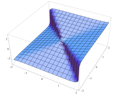
Figure 1: The graph of $z=x+_{1/5}y=(x^{5}+y^{5})^{1/5}$.

2.3 Structures on hyperfields

2.3.1 Orderings and norms

This section also owes much to the paper of Oleg Viro [Vir10].

Definition 2.2.

An ordering on a hyperfield $(F,\odot,\boxplus,1,0)$ is a subset $F_{+}\subset F$ satisfying $F_{+}\boxplus F_{+}\subseteq F_{+}$, $F_{+}\odot F_{+}\subseteq F_{+}$, and $F=F_{+}\coprod\{0\}\coprod-F_{+}$.

An ordering on the sign hyperfield $\mathbb{S}$ is given by $\mathbb{S}_{+}=\{1\}$. An ordering on a hyperfield $F$ determines and is determined by a hyperfield homomorphism $h:F\to\mathbb{S}$ with $F_{+}=h^{-1}\{1\}$.

Orderings on hyperfields pull back, so if $h:F\to F^{\prime}$ is a hyperfield homomorphism and $F^{\prime}_{+}$ is an ordering on $F^{\prime}$, then $h^{*}F^{\prime}_{+}:=h^{-1}F^{\prime}_{+}$ is an ordering on $F$. For any hyperfield $F$, the set of orderings is given by $\{h^{*}\mathbb{S}_{+}:h:F\to\mathbb{S}\}$, where $h$ runs over all hyperfield homomorphisms from $F$ to $\mathbb{S}$.

Categorically speaking, the functor $O:\operatorname{Hyperfield}^{op}\to\operatorname{Set}$ given by the set of orderings on a hyperfield is a representable functor with representing object $\mathbb{S}$. In other words, the pullback gives a natural bijection from $\operatorname{Hyperfield}(-,\mathbb{S})$ to $O(-)$.

Definition 2.3.

A norm on a hyperfield $(F,\odot,\boxplus,1,0)$ is a function $\|~{}\|:F\to\mathbb{R}_{\geq 0}$ satisfying

1. $x\neq 0$ if and only if $\|x\|>0$

2. $\|x\odot y\|=\|x\|\|y\|$

3. $\|x\boxplus y\|\subseteq[0,\|x\|+\|y\|]$

The identity function is a norm on the triangle hyperfield $\triangle$.

Norms on hyperfields pull back, so if $h:F\to F^{\prime}$ is a hyperfield homomorphism and $\|~{}\|$ is a norm on $F^{\prime}$, then $h^{*}\|~{}\|=\|~{}\|\circ h$ is a norm on $F$. We claim that $\triangle$ is a representing object for norms on hyperfields. The key lemma follows.

Lemma 2.4.

Let $F$ be a hyperfield. A function $\|~{}\|:F\to\mathbb{R}_{\geq 0}$ is a norm if and only if $\|~{}\|:F\to\triangle$ is a hyperfield homomorphism.

Proof.

It is clear that if $\|~{}\|:F\to\triangle$ is a hyperfield homomorphism, then $\|~{}\|$ is a norm.

Now suppose that $\|~{}\|:F\to\mathbb{R}_{\geq 0}$ is a norm. Note that in a hyperfield, $-x\odot-x=x\odot x$, which implies that $\|-x\|=\|x\|$. Recall that in the triangle hyperfield, $a\boxplus b=[|a-b|,a+b]$. To prove that $\|~{}\|:F\to\triangle$ is a homomorphism, the only nontrivial part is to show for $x,y,z\in F$, that if $z\in x\boxplus y$, then $|\|x\|-\|y\||\leq\|z\|$. Without loss of generality, $\|x\|\geq\|y\|$.

$$z\in x\boxplus y \Longrightarrow x\in-y\boxplus z$$

$$\Longrightarrow\|x\|\leq\|-y\|+\|z\|=\|y\|+\|z\|$$

$$\Longrightarrow\|x\|-\|y\|\leq\|z\|\qed$$

Thus the set of norms on an arbitrary hyperfield $F$ is given by $\{{h^{*}\|~{}\|_{\triangle}}\}$, where $h$ runs over all hyperfield homomorphisms from $F$ to $\triangle$ and $\|~{}\|_{\triangle}:\triangle\to\mathbb{R}_{\geq 0}$ is the identity function.

Categorically speaking, the functor $N:\operatorname{Hyperfield}^{op}\to\operatorname{Set}$ given by the set of norms on a hyperfield is a representable functor with representing object $\triangle$. In other words, the pullback gives a natural bijection from $\operatorname{Hyperfield}(-,\triangle)$ to $N(-)$.

There is a hyperfield homomorphism $\mathbb{K}\to\triangle$. Thus any hyperfield has a norm by sending $0$ to $0$ and any nonzero element to $1$.

Definition 2.5.

A nonarchimedean norm on a hyperfield $(F,\odot,\boxplus,1,0)$ is a function $\|~{}\|:F\to\mathbb{R}_{\geq 0}$ satisfying

1. $x\neq 0$ if and only if $\|x\|>0$

2. $\|x\odot y\|=\|x\|\|y\|$

3. $\|x\boxplus y\|\subseteq[0,\max\{\|x\|,\|y\|\}]$

The identity function is a nonarchimedean norm on the tropical triangle hyperfield $\mathcal{T}\triangle$.

Nonarchimedean norms on hyperfields were a key motivation for the introduction of hyperfields by Krasner [Kra57]; he used the related notion of a valued hyperfield.

Nonarchimedean norms on hyperfields pull back, so if $h:F\to F^{\prime}$ is a hyperfield homomorphism and $\|~{}\|$ is a nonarchimedean norm on $F^{\prime}$, then $h^{*}\|~{}\|=\|~{}\|\circ h$ is a nonarchimedean norm on $F$. We claim that $\mathcal{T}\triangle$ is a representing object for nonarchimedean norms on hyperfields. The key lemma follows.

Lemma 2.6.

Let $F$ be a hyperfield. A function $\|~{}\|:F\to\mathbb{R}_{\geq 0}$ is a nonarchimedean norm if and only if $\|~{}\|:F\to\mathcal{T}\triangle$ is a hyperfield homomorphism.

Proof.

It is clear that if $\|~{}\|:F\to\mathcal{T}\triangle$ is a hyperfield homomorphism, then $\|~{}\|$ is a nonarchimedean norm.

Now suppose that $\|~{}\|:F\to\mathbb{R}_{\geq 0}$ is a nonarchimedean norm. To prove that $\|~{}\|:F\to\mathcal{T}\triangle$ is a homomorphism, one must show that if $z\in x\boxplus y$, then $\|z\|\in\|x\|\boxplus\|y\|$. This is clear if $\|x\|=\|y\|$.

Thus let’s assume $z\in x\boxplus y$ and $\|x\|>\|y\|$. We wish to show that $\|z\|=\|x\|$.

$$\|z\|\leq\max\{\|x\|,\|y\|\}=\|x\|$$

By reversibility, $x\in-y\boxplus z$. Then

$$\|x\|\leq\max\{\|y\|,\|z\|\}=\|z\|\qed$$

Thus the set of nonarchimedean norms on an arbitrary hyperfield $F$ is given by $\{{h^{*}\|~{}\|}_{\mathcal{T}\triangle}\}$, where $h$ runs over all hyperfield homomorphisms from $F$ to $\mathcal{T}\triangle$ and $\|~{}\|_{\mathcal{T}\triangle}:\mathcal{T}\triangle\to\mathbb{R}_{\geq 0}$ is the identity function.

Categorically speaking, the functor $N:\operatorname{Hyperfield}^{op}\to\operatorname{Set}$ given by the set of nonarchimedean norms on a hyperfield is a representable functor with representing object $\mathcal{T}\triangle$. In other words, the pullback gives a natural bijection from $\operatorname{Hyperfield}(-,\mathcal{T}\triangle)$ to $N(-)$.

There is a hyperfield homomorphism $\mathbb{K}\to\mathcal{T}\triangle$. Thus any hyperfield has a nonarchimedean norm by sending $0$ to $0$ and any nonzero element to $1$.

The function $\operatorname{ph}$ on $\mathbb{C}$ offers the motivating example for the following definition.

Definition 2.7.

An argument on a hyperfield $(F,\odot,\boxplus,1,0)$ is a group homomorphism $\arg:F^{\times}\to S^{1}$ satisfying

1. $\arg(-x)=-\arg(x)$.

2. If $\arg(x)=\arg(y)$, then $\arg(x\boxplus y)=\arg(x)$.

3. If $\arg(x)\neq\pm\arg(y)$ and if $z\in x\boxplus y$, then $\arg(z)$ is on the shortest open arc on the circle connecting $\arg(x)$ and $\arg(y)$.

An argument extends to a function $\arg:F\to S^{1}\cup\{0\}$ by setting $\arg(0)=0$.

We claim that $\mathbb{P}$ is a representing object for arguments on hyperfields. The key lemma follows.

Lemma 2.8.

Let $F$ be a hyperfield. A function $\arg:F^{\times}\to S^{1}$ is an argument if and only if $\arg:F\to\mathbb{P}$ is a hyperfield homomorphism.

Proof.

It is clear that if $\arg:F\to\mathbb{P}$ is hyperfield homomorphism, then $\arg:F^{\times}\to S^{1}$ is an argument.

Now suppose $\arg:F^{\times}\to S^{1}$ is an argument. We need to show that $\arg(x\boxplus y)\subseteq\arg(x)\boxplus\arg(y)$, for each $x,y\in F^{\times}$. The only nontrivial case is when $\arg(y)=\arg(-x)$. By reversibility, if an element $z\in x\boxplus y$, then $y\in z\boxplus-x$. If $\arg(z)$ were not in $\arg(x)\boxplus\arg(y)=\{0,\pm\arg(x)\}$, then $\arg(z\boxplus-x)$ would be contained in the shortest open arc connecting $\arg(z)$ and $\arg(-x)=\arg(y)$. In particular, $\arg(z\boxplus-x)$ would not contain $\arg(y)$, a contradiction. ∎

Definition 2.9.

A $\Phi$-argument on a hyperfield $(F,\odot,\boxplus,1,0)$ is a group homomorphism $\arg:F^{\times}\to S^{1}$ satisfying

1. $\arg(-x)=-\arg(x)$.

2. If $\arg(x)=\arg(y)$, then $\arg(x\boxplus y)=\arg(x)$.

3. If $\arg(x)\neq\pm\arg(y)$ and if $z\in x\boxplus y$, then $\arg(z)$ is on the shortest closed arc on the circle connecting $\arg(x)$ and $\arg(y)$.

An argument is a $\Phi$-argument. Here is an example of a $\Phi$-argument on a field which is not an argument. If $\alpha\in\mathbb{C}$, then a $\Phi$-argument on the rational function field $\mathbb{C}(x)$ is given by $\arg_{\alpha}((x-\alpha)^{n}f(x)/g(x))=\operatorname{ph}(f(\alpha)/g(\alpha))$ where $n$ is an integer and $f$ and $g$ are polynomials which do not have $\alpha$ as a root.

We claim that $\Phi$ is a representing object for $\Phi$-arguments on hyperfields. The key lemma follows.

Lemma 2.10.

Let $F$ be a hyperfield. A function $\arg:F^{\times}\to S^{1}$ is a $\Phi$-argument if and only if $\arg:F\to\Phi$ is a hyperfield homomorphism.

We will omit the proof of this lemma.

This above discussion show a possible utility for the notion of hyperfield. The notions of orderings, norms, nonarchimedean norms, arguments, and $\Phi$-arguments are important for fields, but to find a representing object one needs to leave the category of fields. Likewise, to find a final object one has to leave the category of fields.

Remark 2.11.

Jaiung Jun [Jun17] has studied morphisms to $\mathbb{K}$, $\mathbb{S}$, and $\mathbb{Y}$ from a more general algebro-geometric viewpoint, considering not just sets $\operatorname{Hom}(A,\mathbb{F})$ of morphisms of hyperfields for $\mathbb{F}\in\{\mathbb{K},\mathbb{S},\mathbb{Y}\}$, but also sets $\operatorname{Hom}(\operatorname{Spec}(\mathbb{F}),X)$ of morphisms of hyperring schemes, where $X$ is an algebraic variety (in the classical sense viewed as a hyperring scheme). This recasts the set Hom(A, F) by means of the functor Spec, i.e., Hom(A, F)=Hom(Spec F, Spec A).

2.3.2 Topological hyperfields

Definition 2.12.

A topological hyperfield is a hyperfield $(F,\odot,\boxplus,1,0)$ with a topology $T$ on $F$ satisfying:

1. $F-\{0\}$ is open.

2. Multiplication $F\times F\to F$ is continuous.

3. The multiplicative inverse map $F-\{0\}\to F-\{0\}$ is continuous.

Conditions (2) and (3) guarantee that $(F^{\times},\odot,1)$ is a topological group.

Remark 2.13.

The reader may think it is odd that we do not require addition to be continuous. We do too! But, in our defense: we never need this, and there are several competing notions of continuity of a multivalued map, see Section 8 of [Vir10].

We wish to topologize all of the hyperfields in Diagram (1) so that all the maps are continuous and so that all the dotted arrows are hyperfield homotopy equivalences (defined below). Of course we give $\mathbb{R}$ and $\mathbb{C}$ their usual topologies. We topologize $\triangle$, $\mathbb{S}$, $\mathbb{P}$ and $\mathbb{K}$ as quotients of $\mathbb{R}$ and $\mathbb{C}$, noting that if $F$ is a topological hyperfield and $S$ is a subgroup of $F^{\times}$, then $F\to F/{}_{m}S$ is a morphism of topological hyperfields, where $F/{}_{m}S$ is given the quotient topology. We topologize $\Phi$ so that the identity map $\mathbb{P}\to\Phi$ is a homeomorphism. Thus:

• the topology on $\triangle$ is the same as its topology as a subspace of $\mathbb{R}$.

• the open sets in $\mathbb{S}$ are $\emptyset$, $\{+1\}$, $\{-1\}$, $\{+1,-1\}$, and $\{+1,-1,0\}$.

• the open sets in $\mathbb{P}$ and $\Phi$ are the usual open sets in $S^{1}$ together with the set $S^{1}\cup\{0\}$.

• the open sets in $\mathbb{K}$ are $\emptyset$, $\{1\}$, and $\{0,1\}$.

Although we can give the hyperfields $\mathcal{T}\mathbb{R}$, $\mathcal{T}\mathbb{C}$, and $\mathcal{T}\triangle$ the topologies inherited from the complex numbers, with these topologies many of the maps in Diagram (1) are not continuous, for example, $\mathbb{S}\to\mathcal{T}\mathbb{R}$. Instead we will use the $0$-coarsening described below.

Let $(F,\odot,\boxplus,1,0,T)$ be a topological hyperfield. Define two new topologies ${{}_{0}T}$ and $T_{0}$ on $F$, called the $0$-fine topology and the $0$-coarse topology respectively, with open sets ${{}_{0}T}=\{0\}\cup\{U\in T\}$ and $T_{0}=\{F\}\cup\{U\in T:0\notin U\}$. Thus in ${{}_{0}T}$, $\{0\}$ is an open set, while in $T_{0}$ there are no proper open neighborhoods of $0$. Note that both ${{}_{0}T}$ and $T_{0}$ depend only on the topology on $F^{\times}$, in fact ${{}_{0}T}$ is the finest topology on $F$ which restricts to a fixed topological group $F^{\times}$ and $T_{0}$ is the coarsest. We abbreviate $(F,\odot,\boxplus,1,0,{{}_{0}T})$ by ${{}_{0}F}$ and $(F,\odot,\boxplus,1,0,T_{0})$ by $F_{0}$. For any topological hyperfield $F$, the identity maps ${{}_{0}F}\to F\to F_{0}$ are continuous. A topological hyperfield is $0$-fine if $F={{}_{0}F}$, i.e. $\{0\}$ is an open set. A topological hyperfield is $0$-coarse if $F=F_{0}$, i.e. the only open neighborhood of $0$ is $F$. The hyperfields $\mathbb{S}$, $\mathbb{P}$, $\Phi$, and $\mathbb{K}$ with the topologies described above are $0$-coarse.

We then enrich Diagram (1) to a diagram of topological hyperfields.

(2)

All the maps in the diagram are continuous, and all the dotted arrows are sections of their corresponding solid arrow maps. Note also that for each solid, dotted pair, the target of the solid arrow could be considered both as a quotient and a sub-topological hyperfield of the domain. The authors speculate that dequantization should provide a justification for endowing $\mathcal{T}\mathbb{R}$ with the 0-coarse topology, but we have not been able to make this precise.

Recall that the hyperfield $\mathbb{K}$ is a final object in the category of hyperfields, and that $\mathbb{S}$, $\triangle$, $\mathcal{T}\triangle$, $\mathbb{P}$, and $\Phi$ are representing objects for the set of orderings, norms, nonarchimedean norms, arguments, and $\Phi$-arguments on a given hyperfield. Similar considerations apply to the topological hyperfields. An ordered topological hyperfield $F$ is a topological hyperfield $F$ with an ordering in which $F_{+}$ is an open set. Norms, nonarchimedean norms, arguments, and $\Phi$-arguments on a topological hyperfield are required to be continuous. Then $\mathbb{K}$ is a final object in the category of topological hyperfields and $\mathbb{S}$, $\triangle$, $\mathcal{T}\triangle$, $\mathbb{P}$, and $\Phi$ are representing objects for the set of orderings, norms, nonarchimedean norms, arguments, and $\Phi$-arguments on a given topological hyperfield.

Definition 2.14.

A hyperfield homotopy between topological hyperfields $F$ and $F^{\prime}$ is a continuous function $H:F\times I\to F^{\prime}$ such that, for each $t\in I$, the function $H_{t}:F\to F^{\prime}$ taking $x$ to $H(x,t)$ is a homomorphism of hyperfields.

The following result, which is hardly more than an observation, is fundamental to all of our considerations on Grassmannians and realization spaces associated to hyperfields in Diagram (2).

Proposition 2.15.

Let $F\in\{\triangle_{0},\mathcal{T}\mathbb{R}_{0},\mathcal{T}\mathbb{C}_{0},\mathcal{T}\triangle_{0}\}$. The function $H:F\times I\to F$

$$H(x,t):=\begin{cases}0&x=0\\ x|x|^{-t}&x\neq 0\end{cases}$$

is a hyperfield homotopy.

Note that in each case $H_{0}$ is the identity and $H_{1}$ maps $F$ to $\operatorname{ph}(F)$.

Proof.

Certainly in each case $H$ is continuous, and for all $x$, $y$, and $t$, $H_{t}(x)\odot H_{t}(y)=H_{t}(x\odot y)$.

For the hyperaddition operation on $F\in\{\mathcal{T}\mathbb{R}_{0},\mathcal{T}\mathbb{C}_{0},\mathcal{T}\triangle_{0}\}$ it is clear that $H_{t}(x\boxplus y)=H_{t}(x)\boxplus H_{t}(y)$ for all $x,y,t$.

For the hyperaddition operation on $\triangle_{0}$: consider $x$, $y$, and $z$ such that $z\in x\boxplus y$. Without loss of generality assume $x\geq y>0$. Note that $H_{t}(x)=x^{1-t}=x^{s}$ where $s\in[0,1]$. If $z\in x\boxplus y$, then $x-y\leq z\leq x+y$. We wish to show $x^{s}-y^{s}\leq z^{s}\leq x^{s}+y^{s}$.

Dividing through by $x$ respectively $x^{s}$, it’s enough to show that if $1-a\leq b\leq 1+a$ and $a,b>0$ then $1-a^{s}\leq b^{s}\leq 1+a^{s}$.

To see the first inequality, we write the hypothesis as $1\leq a+b$ and note that:

• if at least one of $a$ and $b$ is greater than or equal to 1, then at least one of $a^{s}$ and $b^{s}$ is greater than or equal to 1, and so $1\leq a^{s}+b^{s}$.

• Otherwise, since $s\in[0,1]$ we have $a^{s}\geq a$ and $b^{s}\geq b$, so $a^{s}+b^{s}\geq a+b\geq 1$.

To see the second inequality: $b\leq 1+a$ implies $b^{s}\leq(1+a)^{s}$. Thus it suffices to show that $(1+a)^{s}\leq 1+a^{s}$, i.e., the function $f(a)=1+a^{s}-(1+a)^{s}$ is nonnegative on $\mathbb{R}_{\geq 0}$. Note $f(0)=0$ and $f^{\prime}(a)=s((a^{s-1}-(1+a)^{s-1})$. Since $0<a<a+1$ and $s-1\leq 0$ we have $a^{s-1}\geq(a+1)^{s-1}$, and so $f$ is increasing on $\mathbb{R}_{\geq 0}$. ∎

Remark 2.16.

Under the bijection $\log:\mathcal{T}\triangle\to\mathbb{Y}$ from the tropical triangle hyperfield to the tropical hyperfield, the homotopy on $\mathcal{T}\triangle_{0}$ given in Proposition 2.15 pushes forward to a straight-line homotopy on $\mathbb{Y}_{0}$.

A homotopy equivalence $h:F\to F^{\prime}$ of topological hyperfields is a continuous hyperfield homomorphism such that there exists a continuous hyperfield homomorphism $g:F^{\prime}\to F$ and hyperfield homotopies $G:F\times I\to F$ and $H:F^{\prime}\times I\to F^{\prime}$ such that $G(x,0)=x$, $G(x,1)=g(h(x))$, $H(x,0)=x$, and $H(x,1)=h(g(x))$. One says that $g$ and $h$ are homotopy inverses. Topological hyperfields $F$ and $F^{\prime}$ are homotopy equivalent if there is a homotopy equivalence between $F$ and $F^{\prime}$.

Returning to Diagram (1), we have the following results about the dotted arrows.

Corollary 2.17.

The following inclusions are homotopy equivalences of topological hyperfields.

1. $\mathbb{K}\hookrightarrow\triangle_{0}$

2. $\mathbb{S}\hookrightarrow\mathcal{T}\mathbb{R}_{0}$

3. $\Phi\hookrightarrow\mathcal{T}\mathbb{C}_{0}$

4. $\mathbb{K}\hookrightarrow\mathcal{T}\triangle_{0}$

In each case, the homotopy inverse is $\operatorname{ph}$.

Proof.

In each case the composition $\operatorname{ph}\circ\text{inc}$ is the identity. The homotopy between the identity and $\text{inc}\circ\operatorname{ph}$ is given in Proposition 2.15. ∎

As we shall see (Theorems 4.4 and 5.6), a hyperfield homotopy induces a homotopy equivalence of Grassmannians, and for each matroid $M$, a hyperfield homotopy between the 0-coarsenings of hyperfields induces a homotopy equivalence of realization spaces of $M$.

For a hyperfield $F$ and a finite set $E$, projective space $\mathbf{P}(F^{E})$ is the quotient of $F^{E}-\{0\}$ by the scalar action of $F^{\times}$. Of course only the cardinality of $E$ is relevant. Cognizant of this, let $F\mathbf{P}^{n-1}=\mathbf{P}(F^{\{1,2,\dots,n\}})$. If $F$ is a topological hyperfield then $F\mathbf{P}^{n-1}$ inherits a topology via the product, subspace, and quotient topologies.

Proposition 2.18.

Let $F$ be a topological hyperfield and $U\subset F^{n}-\{(0,\ldots,0)\}$. If $U$ is open then its image in $F\mathbf{P}^{n-1}$ is open.

Proof.

Let $\pi:F^{n}-\{(0,\ldots,0)\}\to F\mathbf{P}^{n-1}$ be the quotient map. Since multiplication is continuous, the function $x\to\lambda^{-1}\odot x$ from $F$ to $F$ is continuous for each $\lambda\in F^{\times}$, and so $\lambda\odot U$ is open. Thus the union $\bigcup_{\lambda\in F^{\times}}\lambda\odot U$ is open. But this union is $\pi^{-1}(\pi(U))$, and so $\pi(U)$ is open. ∎

In the next section we will define and topologize Grassmann varieties over hyperfields.

3 The Plücker embedding and matroids over hyperfields

Matroids over hyperfields generalize linear subspaces of vector spaces $F^{n}$. For a field $F$, the Grassmannian of $r$-subspaces of $F^{n}$ embeds into projective space via the Plücker embedding $\operatorname{Gr}(r,F^{n})\hookrightarrow F\mathbf{P}^{\binom{n}{r}-1}$. Furthermore the image is an algebraic variety, the zero set of homogenous polynomials called the Grassmann–Plücker relations. Strong and weak $F$-matroids over a hyperfield $F$ are defined in [BB16] in terms of Grassmann–Plücker relations. Strong and weak $F$-matroids coincide when $F$ is a field. We review this theory in Section 3.1 and then use these ideas to define the Grassmannian of a hyperfield in Section 3.2.

3.1 The Plücker embedding

Definition 3.1.

Let $W$ be an $n$-dimensional vector space over a field $F$. Let $\operatorname{Gr}(r,W)$ be the set of $r$-dimensional subspaces of $W$. The Plücker embedding is given by

$$\operatorname{Gr}(r,W) \to\mathbf{P}(\Lambda^{r}W)\cong F\mathbf{P}^{\binom{n}{r}-1}$$

$$V=\text{Span}(v_{1},\dots,v_{r}) \mapsto v_{1}\wedge\dots\wedge v_{r}$$

The fact that $\Lambda^{r}V$ is a rank 1 vector space shows that the above map is independent of the choice of basis for $V$.

More naively, we can see the embedding of $\operatorname{Gr}(r,F^{n})$ into $F\mathbf{P}^{\binom{n}{r}-1}$ in matrix terms. Let $\mathrm{Mat}(r,n)$ be the set of $r\times n$ matrices of rank $r$ over $F$. Thus $GL_{r}(F)$ acts on $\mathrm{Mat}(r,n)$ by left multiplication, and the quotient $GL_{r}(F)\backslash\mathrm{Mat}(r,n)$ is homeomorphic to $\operatorname{Gr}(r,F^{n})$ by the map $GL_{r}(F)M\mapsto\mathop{\mathrm{row}}(M)$, the row space of $M$. For each $\{i_{1},\ldots,i_{r}\}\subseteq[n]=\{1,2,\dots,n\}$ with $i_{1}<\cdots<i_{r}$ and $M\in\mathrm{Mat}(r,n)$ let $|M_{i_{1},\ldots,i_{r}}|$ be the determinant of the submatrix with columns indexed by $\{i_{1},\ldots,i_{r}\}$. Consider the map $P:\mathrm{Mat}(r,n)\to F^{\binom{n}{r}}-\{\mathbf{0}\}$ taking each $M$ to $(|M_{i_{1},\ldots,i_{r}}|)_{\{i_{1},\ldots,i_{r}\}\subseteq[n]}$. Multiplication of $M$ on the left by $A\in GL_{r}(F)$ amounts to a multiplication of $P(M)$ by the determinant of $A$, and so $P$ induces maps

The map $\tilde{P}$ is the Plücker embedding. It is easily seen to be injective: each coset $GL_{r}(F)M$ has a unique element in reduced row-echelon form, and this element can be recovered from $\tilde{P}(M)$.

A point $\vec{x}\in F^{\binom{n}{r}}$ has coordinates $x_{i_{1},\ldots,i_{r}}$ for each $1\leq i_{1}<\cdots<i_{r}\leq n$. To give polynomials defining the image of the Plücker embedding as an algebraic variety, it is convenient to define $x_{i_{1},\ldots,i_{r}}$ for sequences in $[n]$ which are not necessarily increasing, by

$$x_{i_{1},\ldots,i_{r}}=\mathrm{sign}(\sigma)x_{i_{\sigma(1)},\ldots,i_{\sigma(r)}}$$

for each permutation $\sigma$ of $[r]$. (In particular, $x_{i_{1},\ldots,i_{r}}=0$ if the values $i_{j}$ are not distinct.) With this convention we have the following well-known descriptions of the Plücker embedding of the Grassmannian. A proof is found in Chapter VII, Section 6, of [HP47].

Throughout the following the notation $i_{1},\ldots,\widehat{i_{k}},\ldots,i_{r+1}$ means that the term $i_{k}$ is omitted.

Proposition 3.2.

Let $F$ be a field.

1. (The Grassmann–Plücker relations) The image of $\tilde{P}$ is exactly the set of $\vec{x}$ satisfying the following. For each $I=\{i_{1},\ldots,i_{r+1}\}\subseteq[n]$ and each $J=\{j_{1},\ldots,j_{r-1}\}\subseteq[n]$,

   $$\sum_{k=1}^{r+1}(-1)^{k}x_{i_{1},\ldots,\widehat{i_{k}},\ldots,i_{r+1}}x_{i_{k},j_{1},\ldots,j_{r-1}\vphantom{\widehat{i_{k}}}}=0$$ (3)

2. (Weak Grassmann–Plücker conditions) The image of $\tilde{P}$ is exactly the set of $\vec{x}$ satisfying:

   1. $\{\{k_{1},\ldots,k_{r}\}\subseteq[n]:x_{k_{1},\ldots,k_{r}}\neq 0\}$ is the set of bases of a matroid, and

   2. Equation (3) holds for all $I$ and $J$ with $|I-J|=3$.

The second weak Grassmann–Plücker condition is known as the 3-term Grassmann–Plücker relations.

Example 3.3.

Let $V$ be a 2-dimensional subspace of a 4-dimensional vector space $W$. Let $\{v_{1},v_{2}\}$ be a basis for $V$ and $\{e_{1},e_{2},e_{3},e_{4}\}$ be a basis for $W$. Let

$$v_{1}\wedge v_{2}=\ x_{12}\ e_{1}\wedge e_{2}+x_{13}\ e_{1}\wedge e_{3}+x_{14}\ e_{1}\wedge e_{4}$$

$$+x_{34}\ e_{3}\wedge e_{4}+x_{24}\ e_{2}\wedge e_{4}+x_{23}\ e_{2}\wedge e_{3}$$ (4)

Then since $v_{1}\wedge v_{2}\wedge v_{1}\wedge v_{2}=0$, the coordinates satisfy the homogenous quadratic equation

$$x_{12}x_{34}-x_{13}x_{24}+x_{14}x_{23}=0.$$ (5)

Conversely, given a nonzero solution to (5), there are vectors $v_{1}$ and $v_{2}$ satisfying (3.3). One can reason as follows. One of the $x_{ij}$ is nonzero, so without loss of generality we may assume $x_{12}=1$. If $v_{1}=e_{1}-x_{23}e_{3}-x_{34}e_{4}$ and $v_{2}=e_{2}+x_{13}e_{3}+x_{24}e_{4}$, then (3.3) is satisfied.

Thus for a field $K$ the image of the Plücker embedding of $\operatorname{Gr}(2,K^{4})$ is the projective variety given by the 3-term Grassmann–Plücker relations with $I=\{2,3,4\}$ and $J=\{1\}$.

When the field in Proposition 3.2 is replaced by a hyperfield, things go haywire. There are $\vec{x}$ satisfying the hyperfield analog of the weak Grassmann–Plücker conditions, but which do not satisfy the hyperfield analog to the general Grassmann–Plücker relations. The 3-term Grassmann–Plücker relations lead to the notion of a weak $F$-matroid, while the general Grassmann–Plücker relations lead to the notion of a strong $F$-matroid.

3.2 Matroids over hyperfields

Definition 3.4.

[BB16] Let $F$ be a hyperfield. Let $E$ be a finite set. A Grassmann–Plücker function of rank $r$ on $E$ with coefficients in $F$ is a function $\varphi:E^{r}\to F$ such that

• $\varphi$ is not identically zero.

• $\varphi$ is alternating.

• (Grassmann–Plücker Relations) For any $(i_{1},\dots,i_{r+1})\in E^{r+1}$ and $(j_{1},\dots,j_{r-1})\in E^{r-1}$,

  $$0\in\mathop{\vphantom{\bigoplus}\mathchoice{\vbox{\hbox{\leavevmode\resizebox{0.0pt}{}{$\boxplus$}}}}{\vbox{\hbox{\leavevmode\resizebox{0.0pt}{}{$\boxplus$}}}}{\vbox{\hbox{\leavevmode\resizebox{0.0pt}{}{$\boxplus$}}}}{\vbox{\hbox{\leavevmode\resizebox{0.0pt}{}{$\boxplus$}}}}}\displaylimits_{k=1}^{r+1}(-1)^{k}\varphi(i_{1},\ldots,\widehat{i_{k}},\ldots,i_{r+1})\odot\varphi({i_{k},j_{1},\ldots,j_{r-1}})$$

Two functions $\varphi_{1},\varphi_{2}:E^{r}\to F$ are projectively equivalent if there exists $\alpha\in F^{\times}$ such that $\varphi_{1}=\alpha\odot\varphi_{2}$.

Example 3.5.

Let $E$ be a finite subset of a vector space over a field $K$ with $\dim_{K}\operatorname{Span}E=r$. Then a Grassmann–Plücker function of rank $r$ on $E$ with coefficients in the Krasner hyperfield $\mathbb{K}$ is given by defining $\varphi(i_{1},\dots,i_{r})$ to be zero if $\{i_{1},\dots,i_{r}\}$ is linearly dependent and one if $\{i_{1},\dots,i_{r}\}$ is linearly independent. The projective equivalence class determines a rank $r$ matroid for which $E$ is a representation over $K$. (Because $|\mathbb{K}^{\times}|=1$, each projective equivalence class has only one element.)

Definition 3.6.

[BB16] A strong $F$-matroid of rank $r$ on $E$ is the projective equivalence class of a Grassmann–Plücker function of rank $r$ on $E$ with coefficients in $F$.

Definition 3.7.

[BB16] Let $F$ be a hyperfield. Let $E$ be a finite set. A weak Grassmann–Plücker function of rank $r$ on $E$ with coefficients in $F$ is a function $\varphi:E^{r}\to F$ such that

• $\varphi$ is not identically zero.

• $\varphi$ is alternating

• The sets $\{i_{1},\dots,i_{r}\}$ for which $\varphi(i_{1},\dots i_{r})\neq 0$ form the set of bases of a ordinary matroid. Equivalently, if $\kappa:F\to\mathbb{K}$ is the unique hyperfield homomorphism to the Krasner hyperfield, then $\kappa\circ\varphi$ is a Grassmann–Plücker function of rank $r$ on $E$ with coefficients in $\mathbb{K}$.

• (3-term Grassmann–Plücker Relations) For any $I=(i_{1},\dots,i_{r+1})\in E^{r+1}$ and $J=(j_{1},\dots,j_{r})\in E^{r-1}$ for which $|I-J|=3$,

  $$0\in\mathop{\vphantom{\bigoplus}\mathchoice{\vbox{\hbox{\leavevmode\resizebox{0.0pt}{}{$\boxplus$}}}}{\vbox{\hbox{\leavevmode\resizebox{0.0pt}{}{$\boxplus$}}}}{\vbox{\hbox{\leavevmode\resizebox{0.0pt}{}{$\boxplus$}}}}{\vbox{\hbox{\leavevmode\resizebox{0.0pt}{}{$\boxplus$}}}}}\displaylimits_{k=1}^{r+1}(-1)^{k}\varphi(i_{1},\ldots,\widehat{i_{k}},\ldots,i_{r+1})\odot\varphi({i_{k},j_{1},\ldots,j_{r-1}})$$

Definition 3.8.

[BB16] A weak $F$-matroid of rank $r$ on $E$ is the projective equivalence class of a weak Grassmann–Plücker function of rank $r$ on $E$ with coefficients in $F$.

Note that a strong $F$-matroid is a weak $F$-matroid. Baker and Bowler show that if a hyperfield satisfies the doubly distributive property, then weak and strong $F$-matroids coincide. The hyperfields in Diagram (1) which are doubly distributive are $\mathbb{R}$ and $\mathbb{C}$ (because they are fields), $\mathbb{S}$ and $\mathbb{K}$ (Section 4.5 in [Vir10]), $\mathcal{T}\mathbb{R}$ (Section 7.2 in [Vir10]), and $\mathcal{T}\triangle$ (Section 5.2 in [Vir10]). For each of the remaining hyperfields, strong matroids and weak matroids do not coincide:

• Example 3.30 in [BB16] is a weak $\triangle$-matroid which is not strong.

• Example 3.31 in [BB16], which is due to Weissauer, is a function $\varphi$ from 3-tuples from a 6-element set to $S^{1}\cup\{0\}$. Viewing $S^{1}\cup\{0\}$ as contained in the underlying set of a hyperfield $F\in\{\mathbb{P},\Phi,\mathcal{T}\mathbb{C}\}$, this $\varphi$ is the Grassmann–Plücker function of a weak $F$-matroid which is not strong.

When dealing with hyperfields for which weak and strong matroids coincide, we will leave out the adjectives “weak” and “strong.”

A $\mathbb{K}$-matroid is a matroid and an $\mathbb{S}$-matroid is an oriented matroid. As we have seen, when $F$ is a field, an $F$-matroid is the image of a subspace of $F^{E}$ under the Plücker embedding.

It is also possible to interpret strong $F$-matroids as generalizations of linear subspaces in a more direct way. Associated to a strong $F$-matroid of rank $r$ on $E$ is a set ${\mathcal{V}}^{*}\subseteq F^{E}$, called the set of $F$-covectors of the $F$-matroid. If $F$ is a field, and thus an $F$-matroid is the Plücker embedding of a subspace $V$ of $F^{E}$, then the $F$-covectors of the $F$-matroid are exactly the elements of $V$. See [And19] for details.

4 Hyperfield Grassmannians

Definition 4.1.

The strong Grassmannian $\operatorname{Gr}^{s}(r,F^{E})$ is the set of strong $F$-matroids of rank $r$ on $E$. The weak Grassmannian $\operatorname{Gr}^{w}(r,F^{E})$ is the set of weak $F$-matroids of rank $r$ on $E$. We use the notation $\operatorname{Gr}^{*}(r,F^{n})$, where $*\in\{s,w\}$.

Remark 4.2.

$\operatorname{Gr}^{s}(r,F^{E})$ is called the $F$-Grassmannian in [BB16].

Remark 4.3.

We abbreviate $\operatorname{Gr}^{*}(r,F^{\{1,\dots,n\}})$ by $\operatorname{Gr}^{*}(r,F^{n})$. If $E$ has cardinality $n$, then introducing a total order on $E$ gives a bijection $\operatorname{Gr}^{*}(r,F^{E})\cong\operatorname{Gr}^{*}(r,F^{n})$.

Note that

$$\operatorname{Gr}^{s}(r,F^{n})\subset\operatorname{Gr}^{w}(r,F^{n})\subset\mathbf{P}(F^{n^{r}})$$

If $F$ is a topological hyperfield, then each of the sets above inherits a topology. For a topological hyperfield there is a stabilization embedding

$$\operatorname{Gr}^{*}(r,F^{n}) \hookrightarrow\operatorname{Gr}^{*}(r,F^{n+1})$$

$$[\varphi:\{1,\dots,n\}^{r}\to F] \mapsto[{\widehat{\varphi}}:\{1,\dots,n+1\}^{r}\to F]$$

given by considering $\{1,\dots,n\}^{\{1,\dots,r\}}\subset\{1,\dots,n+1\}^{\{1,\dots,r\}}$ and defining ${\widehat{\varphi}}$ to be equal to $\varphi$ on the subset and zero on the complement. We then define $\operatorname{Gr}^{*}(r,F^{\infty})$ as the colimit of $\operatorname{Gr}^{*}(r,F^{n})$ as $n\to\infty$. In other words, $\operatorname{Gr}^{*}(r,F^{\infty})$ is the union of $\operatorname{Gr}^{*}(r,F^{n})$, and a subset of $\operatorname{Gr}^{*}(r,F^{\infty})$ is open if and only if its intersection with $\operatorname{Gr}^{*}(r,F^{n})$ is open for all $n$.

A continuous homomorphism $h:F\to F^{\prime}$ of topological hyperfields induces a continuous map

$$\operatorname{Gr}^{*}(h):\operatorname{Gr}^{*}(r,F^{n}) \to\operatorname{Gr}^{*}(r,F^{\prime\,n})$$

$$[\varphi] \mapsto[h\circ\varphi]$$

The following theorem follows from the definitions, but is nonetheless powerful.

Theorem 4.4.

Let $H:F\times I\to F^{\prime}$ be a hyperfield homotopy. Define

$$\operatorname{Gr}^{*}(H):\operatorname{Gr}^{*}(r,F^{n})\times I\to\operatorname{Gr}^{*}(r,F^{\prime\,n})$$

by $\operatorname{Gr}^{*}(H)([\varphi],t)=\operatorname{Gr}^{*}(H_{t})([\varphi])$. Then $\operatorname{Gr}^{*}(H)$ is continuous.

If $F$ and $F^{\prime}$ are homotopy equivalent, then so are the topological spaces $\operatorname{Gr}^{*}(r,F^{n})$ and $\operatorname{Gr}^{*}(r,F^{\prime\,n})$.

From Proposition 2.17 we see:

Corollary 4.5.

1. $\operatorname{Gr}(r,\mathbb{S}^{n})\simeq\operatorname{Gr}(r,\mathcal{T}\mathbb{R}_{0}^{n})$

2. $\operatorname{Gr}^{*}(r,\Phi^{n})\simeq\operatorname{Gr}^{*}(r,\mathcal{T}\mathbb{C}_{0}^{n})$ for $*\in\{s,w\}$

3. $\operatorname{Gr}(r,\mathbb{K}^{n})\simeq\operatorname{Gr}^{*}(r,\triangle_{0}^{n})$ for $*\in\{s,w\}$

4. $\operatorname{Gr}(r,\mathbb{K}^{n})\simeq\operatorname{Gr}(r,\mathcal{T}\triangle_{0}^{n})$

Part 1 of this corollary gives us the homotopy equivalence referred to in Part 2 of Theorem 1.1. As will be discussed in Section 6, $\operatorname{Gr}(r,\mathbb{K}^{n})$ is contractible, and $\operatorname{Gr}(r,\mathbb{S}^{n})$ is the MacPhersonian $\mathrm{MacP}(r,n)$.

5 Realization spaces

For any morphism of hyperfields $f:F\to F^{\prime}$ and $*\in\{s,w\}$, we get a partition of $\operatorname{Gr}^{*}(r,F^{n})$ into preimages under $\operatorname{Gr}^{*}(f)$. The preimage of $M\in\operatorname{Gr}^{*}(r,F^{\prime\,n})$ will be denoted $\operatorname{Real}_{F}^{*}(M)$, and if $F$ is a topological hyperfield then $\operatorname{Real}_{F}^{*}(M)$ is the (strong or weak) realization space of $M$ over $F$. An element of $\operatorname{Real}_{F}^{*}(M)$ is called a (strong or weak) realization of $M$ over $F$. An $F^{\prime}$-matroid is (strong or weak) realizable over $F$ if it has a (strong or weak) realization over $F$. (This is a rephrasing of Definition 4.9 in [BB16].) When dealing with hyperfields for which weak and strong coincide, we will leave out the adjectives “weak” and “strong” and write simply $\operatorname{Real}_{F}(M)$.

Example 5.1.

Recall that a $\mathbb{K}$-matroid is simply called a matroid. For any hyperfield $F$, there is a unique morphism $\kappa:F\to\mathbb{K}$. We call the resulting partition of $\operatorname{Gr}^{*}(r,F^{n})$ the matroid partition. The realization space $\operatorname{Real}_{F}^{*}(M)$ is exactly the set of (strong or weak) rank $r$ $F$-matroids on $[n]$ whose Grassmann–Plücker functions are nonzero exactly on the ordered bases of the matroid $M$.

Example 5.2.

If $F=\mathbb{S}$ and $M$ is a matroid then $\operatorname{Real}_{F}(M)$ is the set of orientations of $M$; this has been much-studied (cf. Section 7.9 in [BLVS⁺99]).

Example 5.3.

Let $M$ be a matroid and let $\mathbb{Y}$ be the tropical hyperfield, i.e., the hyperfield on elements $\mathbb{R}\cup\{-\infty\}$ with operations induced by the bijection $\log:\mathcal{T}\triangle\to\mathbb{R}\cup\{-\infty\}$. Then $\operatorname{Real}_{\mathbb{Y}}(M)$ is essentially the Dressian $\mathrm{Dr}_{M}$ discussed in [MS15]. More precisely, assume $M$ is a matroid $\varphi:E^{r}\to\mathbb{K}$ and ${\mathcal{B}}=\{\{i_{1},\ldots i_{r}\}:\varphi(i_{1},\ldots,i_{r})=1\}$. (In standard matroid language, $\mathcal{B}$ is the set of bases of $M$.) Then we have an embedding

$$\operatorname{Real}_{\mathbb{Y}}(M) \to\mathbb{R}^{\mathcal{B}}/\mathbb{R}(1,\ldots,1)$$ (6)

$$[\hat{\varphi}] \to[(\hat{\varphi}(i_{1},\ldots,i_{r}):\{i_{1},\ldots,i_{r}\}\in\mathcal{B})]$$ (7)

$$\operatorname{Real}_{\mathbb{Y}}(M) \to\mathbb{R}^{\cal B}/\mathbb{R}(1,\ldots,1)$$ (8)

$$[\hat{\varphi}] \to[(\hat{\varphi}(i_{1},\ldots,i_{r}):\{i_{1},\ldots,i_{r}\}\in\cal B)]$$ (9)

whose image is $\mathrm{Dr}_{M}$.

In particular, if $M$ is the uniform rank $r$ matroid on $n$ elements then $\operatorname{Real}_{\mathbb{Y}}(M)={\mathrm{D}r}(r,n)$. (Recall that the uniform matroid of rank $r$ on elements $E$ is the matroid in which each $r$-element subset of $E$ is a basis, or equivalently, the $\mathbb{K}$-matroid whose Grassmann–Plücker function $\varphi:E^{r}\to\mathbb{K}$ takes every $r$-tuple of distinct elements to 1.)

Realization spaces of matroids and oriented matroids over fields is a rich subject (cf. Ch. 6 in [Oxl11], [Zie96], [Rui13]). Even determining whether a given matroid or oriented matroid is realizable over a particular field is a nontrivial task. Most matroids and most oriented matroids are not realizable over $\mathbb{R}$ (Corollary 7.4.3 in [BLVS⁺99]), and the realization space of an oriented matroid over $\mathbb{R}$ (or a phased matroid over $\mathbb{C}$) can have horrendous topology [Mnë88].

5.1 Topology of realization spaces

Lemma 5.4.

Let $f:F\to F^{\prime}$ be a morphism of hyperfields. Let $F_{1}$ and $F_{2}$ be topological hyperfields with underlying hyperfield $F$ such that the identity map $F_{1}\to F_{2}$ restricts to a homeomorphism on each preimage $f^{-1}(a)$. Let $M\in\operatorname{Gr}^{*}(r,F^{\prime\,n})$. Then the identity maps

$$\operatorname{Real}^{*}_{F_{1}}(M)\to\operatorname{Real}^{*}_{F_{2}}(M)$$

are homeomorphisms.

Proof.

Consider a basis $\{b_{1},\ldots,b_{r}\}$ for $M$, i.e. a set such that each Grassmann–Plücker function for $M$ is nonzero on $(b_{1},\ldots,b_{r})$. Fix $\varphi^{\prime}$ to be the unique Grassmann–Plücker function for $M$ such that $\varphi^{\prime}(b_{1},\ldots,b_{r})=1$. The map $\varphi\to[\varphi]$ from $P=\{\varphi\in F^{[n]^{r}}:[\varphi]\in\operatorname{Real}_{F}(M)\mbox{ and }\varphi(b_{1},\ldots,b_{r})=1\}$ to $\operatorname{Real}_{F}(M)$ is a homeomorphism, by Proposition 2.18. But $P$ is a subset of the Cartesian product

$$\prod_{(c_{1},\ldots,c_{r})\in[n]^{r}}f^{-1}(\varphi^{\prime}(c_{1},\ldots,c_{r}))$$

whose topology is the same in $F_{1}$ and $F_{2}$. ∎

Corollary 5.5.

Let $f:F\to F^{\prime}$ be a morphism of hyperfields, let $M$ be an $F^{\prime}$-matroid, and let $F$ be a topological hyperfield. Then the identity maps

$$\operatorname{Real}^{*}_{{{}_{0}F}}(M)\to\operatorname{Real}^{*}_{F}(M)\to\operatorname{Real}^{*}_{F_{0}}(M)$$

are homeomorphisms.

Proof.

For $a\in F^{\prime}$, either $f^{-1}(a)=\{0\}$ or $f^{-1}(a)\subseteq F-\{0\}$. If $F$ is a topological hyperfield, then the three topologies ${}_{0}F$, $F$, and $F_{0}$ induce the same topology on $F-\{0\}$ and on $\{0\}$, and hence on $f^{-1}(a)$. Lemma 5.4 applies. ∎

Theorem 5.6.

Let $F$ and $F^{\prime}$ be topological hyperfields and let $F^{\prime\prime}$ be a hyperfield. Let $f:F\to F^{\prime\prime}$ and $f^{\prime}:F^{\prime}\to F^{\prime\prime}$ be hyperfield morphisms. Let $M$ be a $F^{\prime\prime}$-matroid. If $H:F_{0}\times I\to F^{\prime}_{0}$ is a hyperfield homotopy such that $f^{\prime}(H(x,t))=f(x)$ for all $x$ and $t$, then $H$ induces a homotopy $\operatorname{Real}_{F}^{*}(M)\times I\to\operatorname{Real}_{F^{\prime}}^{*}(M)$.

Proof.

We have a commutative diagram

(10)

where $\operatorname{Gr}^{*}(H)$ is the homotopy of Theorem 4.4 and the southeast map sends each $(M,t)$ to $\operatorname{Gr}^{*}(f)(M)$. Thus $\operatorname{Gr}^{*}(H)$ restricts to a map $\operatorname{Real}_{F_{0}}(M)\times I\to\operatorname{Real}_{F_{0}^{\prime}}(M)$, which by Corollary 5.5 is our desired homotopy. ∎

Applying this to the homotopies in Proposition 2.15, and in stark contrast to the situation with realizations over $\mathbb{R}$ and $\mathbb{C}$, we have the following.

Corollary 5.7.

1. For any matroid $M$, $\operatorname{Real}_{\triangle}^{*}(M)$ and $\operatorname{Real}_{\mathcal{T}\triangle}(M)$ are contractible.

2. For any oriented matroid $M$, $\operatorname{Real}_{\mathcal{T}\mathbb{R}}(M)$ is contractible.

3. For every $M\in\operatorname{Gr}^{*}(r,\Phi^{n})$, $\operatorname{Real}_{\mathcal{T}\mathbb{C}}^{*}(M)$ is contractible.

In particular, each of these realization spaces is nonempty: that is, every matroid is realizable over $\triangle$ and $\mathcal{T}\triangle$, every oriented matroid is realizable over $\mathcal{T}\mathbb{R}$, and every (strong or weak) phased matroid is realizable over $\mathcal{T}\mathbb{C}$. This much is actually easy to see even without Theorem 5.6. For instance, notice that $\mathbb{K}$ is a subhyperfield of $\triangle$, and so the Grassmann–Plücker function of a $\mathbb{K}$-matroid $M$ can also be viewed as the Grassmann–Plücker function of a $\triangle$-matroid realizing $M$, and likewise for $\mathbb{K}\subset\mathcal{T}\triangle$, $\mathbb{S}\subset\mathcal{T}\mathbb{R}$, and $\Phi\subset\mathcal{T}\mathbb{C}$.

5.2 Gluing realization spaces

One approach to understanding the topology of a Grassmannian $Gr^{*}(r,F^{n})$ is to understand the realization spaces arising from a hyperfield morphism $F\to F^{\prime}$ and then to understand how these realization spaces “glue together” – that is, to understand intersections $\overline{\operatorname{Real}^{*}_{F}(M)}\cap\operatorname{Real}^{*}_{F}(M^{\prime})$. Here $\overline{S}$ denotes the topological closure of a set $S$. Two key observations are contained in the following.

Proposition 5.8.

1. Let $f:F\to F^{\prime}$ be a morphism of topological hyperfields and $S\subseteq\operatorname{Gr}^{*}(r,F^{\prime\,n})$. Then

$$\overline{\bigcup_{M\in S}\operatorname{Real}^{*}_{F}(M)}\subseteq\bigcup_{M^{\prime}\in\overline{S}}\operatorname{Real}^{*}_{F}(M^{\prime}).$$

2. There is an $M\in\operatorname{Gr}(3,\mathbb{S}^{7})$ such that

$$\emptyset\neq\overline{\operatorname{Real}_{\mathbb{R}}(M)}\subsetneq\bigcup_{M^{\prime}\in\overline{\{M\}}}\operatorname{Real}_{\mathbb{R}}(M^{\prime}).$$

Proof.

1. $\operatorname{Gr}^{*}(r,F^{n})-\bigcup_{M^{\prime}\in\overline{S}}\operatorname{Real}^{*}_{F}(M)$ is the preimage of the open set $\operatorname{Gr}^{*}(r,F^{\prime\,n})-\overline{S}$ under the continuous map $\operatorname{Gr}^{*}(f)$, hence is open. Thus $\bigcup_{M^{\prime}\in\overline{S}}\operatorname{Real}^{*}_{F}(M)$ is a closed set containing $\bigcup_{M\in S}\operatorname{Real}^{*}_{F}(M)$.

2. Figure 2.4.4 in [BLVS⁺99] shows oriented matroids $M_{1},M_{2}\in G(3,\mathbb{S}^{7})$ such that $M_{2}\in\overline{\{M_{1}\}}$ but $\emptyset\neq\operatorname{Real}_{\mathbb{R}}(M_{2})\nsubseteq\overline{\operatorname{Real}_{\mathbb{R}}(M_{1})}$. ∎

The first part of Proposition 5.8 suggests an appealing approach when $F^{\prime}$ is $\mathbb{K}$ or $\mathbb{S}$, since closures in $\operatorname{Gr}(r,\mathbb{K}^{n})$ and $\operatorname{Gr}(r,\mathbb{S}^{n})$ have simple combinatorial descriptions: each of these Grassmannians is finite and has a poset structure, described in Section 6, and the closure of $\{M\}$ is just the set of elements less than or equal to $M$. Thus one can hope to construct $\operatorname{Gr}^{*}(r,F^{n})$ by attaching realization spaces of successively greater $F^{\prime}$-matroids, similarly to how one constructs a CW complex by constructing successively higher-dimensional skeleta. However, as the second part of the proposition suggests, the attaching maps can be messy and are poorly understood.

If $F_{1}$ is a coarsening of $F_{2}$, $F_{2}\stackrel{{\scriptstyle\mathrm{id}}}{{\to}}F_{1}\to F$ are morphisms of topological hyperfields, and $M$ is an $F$-matroid, then $\overline{\operatorname{Real}^{*}_{F_{1}}(M)}\supseteq\overline{\operatorname{Real}^{*}_{F_{2}}(M)}$. Thus realization spaces are “glued more” over $F_{1}$ – i.e., $\overline{\operatorname{Real}_{F_{1}}(M)}\cap\operatorname{Real}_{F_{1}}(M^{\prime})\supseteq\overline{\operatorname{Real}_{F_{2}}(M)}\cap\operatorname{Real}_{F_{2}}(M^{\prime})$ for all $M$ and $M^{\prime}$ – and $F_{1}$ offers a better chance than $F_{2}$ of satisfying $\overline{\operatorname{Real}^{*}_{F_{i}}(M)}=\bigcup_{M^{\prime}\in\overline{\{M\}}}\operatorname{Real}_{F_{i}}(M)$. In particular, if $F$ is a topological hyperfield then the Grassmannians $\operatorname{Gr}^{*}(r,{{}_{0}F}^{n})$, $\operatorname{Gr}^{*}(r,F^{n})$, and $\operatorname{Gr}^{*}(r,F_{0}^{n})$ are constructed from the same realization spaces, glued together most strongly in $\operatorname{Gr}^{*}(r,F_{0}^{n})$, and, as Proposition 5.9 will show, not glued together at all in $\operatorname{Gr}^{*}(r,{{}_{0}F}^{n})$. This suggests the possibility of studying the partition of a Grassmannian into realization spaces by tinkering with neighborhoods of 0 to improve the gluing.

The realization space of the uniform matroid of rank $r$ on elements $E$ is just the set of all elements of $\operatorname{Gr}^{*}(r,F^{E})$ with all Plücker coordinates nonzero. This implies that if $M$ is the uniform matroid, then the realization space $\operatorname{Real}_{F}^{*}(M)$ is open in the $F$-Grassmannian. (This set may be empty: for instance, the uniform rank 2 matroid on elements $\{1,2,3,4\}$ is not realizable over the field $\mathbb{F}_{2}$.) As the following proposition shows, either this is the only open part of the matroid partition or every part is open (and hence $\operatorname{Gr}^{*}(r,F^{E})$ is a topological disjoint union of the parts of $\operatorname{Real}_{F}^{*}(M)$).

Proposition 5.9.

Let $F$ be a topological hyperfield. The following are equivalent.

1. $\{0\}$ is open in $F$.

2. For every rank $r$ matroid $M$ on $n$ elements, the realization space $\operatorname{Real}_{F}^{*}(M)$ is open in the $F$-Grassmannian $\operatorname{Gr}^{*}(r,F^{n})$.

3. For every rank $r$ matroid $M$ on $n$ elements, $\overline{\operatorname{Real}_{F}^{*}(M)}=\operatorname{Real}_{F}^{*}(M)$.

4. There exists an $r$ and $n$ and a nonuniform rank $r$ matroid $M$ on $n$ elements, such that $\operatorname{Real}_{F}^{*}(M)$ is nonempty and open in the $F$-Grassmannian $\operatorname{Gr}^{*}(r,F^{n})$.

Examples of topological hyperfields in which $\{0\}$ is open are $\mathbb{P}$ and $\Phi$ topologized as subspaces of $\mathbb{C}$.

Lemma 5.10.

Let $F$ be a hyperfield and $A=\{a_{1},\ldots,a_{r+1}\}$.

1. Every nonzero alternating function $A^{r}\to F$ is a Grassmann–Plücker function.

2. The function $\operatorname{Gr}(r,F^{A})\to F\mathbf{P}^{r}$ taking $[\varphi]$ to $[\varphi(a_{1},\ldots,\hat{a_{i}},\ldots,a_{r+1})]_{i\in[r+1]}$ is a homeomorphism.

Proof.

1. In this case the Grassmann–Plücker relations are trivial.

2. Let $\operatorname{Alt}(A^{r},F)$ be the set of alternating functions from $A^{r}$ to $F$, topologized as a subset of $F^{A^{r}}$. There are inverse continuous maps

$$\operatorname{Alt}(A^{r},F) \cong F^{A}$$

$$\varphi \mapsto(a_{i}\mapsto\varphi(a_{1},\ldots,{\widehat{a_{i}}},\ldots,a_{r+1}))$$

$$(\varphi(a_{1},\ldots,{\widehat{a_{i}}},\ldots,a_{r+1})=f(a_{i})) \mapsfrom f,$$

which descend to homeomorphisms after projectivizing. ∎

Lemma 5.11.

Let $F$ be a topological hyperfield, $M$ a rank $r$ matroid on a finite set $E$ such that $\operatorname{Real}_{F}^{*}(M)$ is nonempty, and $A\subseteq E$ an $(r+1)$-element subset. Then any alternating function $\tilde{\varphi}:A^{r}\to F$ which is nonzero exactly on the ordered bases of $M$ contained in $A$ extends to a Grassmann–Plücker function $\varphi:E^{r}\to F$ such that $[\varphi]\in\operatorname{Real}_{F}^{*}(M)$.

Proof.

Let $A=\{a_{1},\dots,a_{r+1}\}$. Let $\varphi_{0}:E^{r}\to F$ be the Grassmann–Plücker function of some element of $\operatorname{Real}_{F}^{*}(M)$. Let

$$D=\bigodot_{i}\frac{\varphi_{0}(a_{1},\ldots,\widehat{a_{i}},\ldots,a_{r+1})}{\tilde{\varphi}(a_{1},\ldots,\widehat{a_{i}},\ldots,a_{r+1})}$$

where the product is over all $i$ such that $\tilde{\varphi}(a_{1},\ldots,\widehat{a_{i}},\ldots,a_{r+1})\neq 0$. For each $e\in E$ define $\lambda_{e}$ by

$$\lambda_{e}=\begin{cases}\frac{\varphi_{0}(a_{1},\ldots,\widehat{a_{i}},\ldots,a_{r+1})}{\tilde{\varphi}(a_{1},\ldots,\widehat{a_{i}},\ldots,a_{r+1})}&\text{ if $e=a_{i}$ and $\tilde{\varphi}(a_{1},\ldots,\widehat{a_{i}},\ldots,a_{r+1})\neq 0$}\\ 1&\mbox{ otherwise}\end{cases}$$

Define $\varphi:E^{r}\to F$ by

$$\varphi(e_{1},\ldots,e_{r})=D^{-1}(\bigodot_{i=1}^{r}\lambda_{e_{i}})\varphi_{0}(e_{1},\ldots,e_{r})$$

One easily checks that $\varphi$ and $\tilde{\varphi}$ coincide on $A^{r}$. The Grassmann–Plücker relations for $\varphi_{0}$ imply the Grassmann–Plücker relations for $\varphi$; thus $\varphi$ is an $F$-matroid. Also, the functions $\varphi$ and $\varphi_{0}$ have the same zeroes, so $[\varphi]\in\operatorname{Real}_{F}^{*}(M)$. ∎

Lemma 5.12.

Let $F$ be a topological hyperfield, $E$ a finite set, and $B$ an ordered $r$-tuple from $E$.

1. $\operatorname{Gr}^{*}(r,F^{E})_{B}=\{[\varphi]\in\operatorname{Gr}^{*}(r,F^{E}):\varphi(B)\neq 0\}$ is an open subset of $\operatorname{Gr}^{*}(r,F^{E})$.

2. For any $A\supseteq B$, the restriction map $\operatorname{Gr}^{*}(r,F^{E})_{B}\to\operatorname{Gr}^{*}(r,F^{A})_{B}$ is an open map.

Proof.

1. Since $F\backslash\{0\}$ is open, $\{\varphi\in F^{E^{r}}:\varphi(B)\neq 0\}$ is open in $F^{E^{r}}$. Proposition 2.18 says that $F^{E^{r}}\backslash\{0\}\to\mathbf{P}(F^{E^{r}})$ is an open map; thus $\{[\varphi]\in\mathbf{P}(F^{E^{r}}):\varphi(B)\neq 0\}$ is open in $\mathbf{P}(F^{E^{r}})$. The result follows by intersecting with the Grassmannian.

2. Projection maps are open, and so the map $\{\varphi\in F^{E^{r}}:\varphi(B)\neq 0\}\to\{\varphi\in F^{A^{r}}:\varphi(B)\neq 0\}$ is open. Thus the map $\{[\varphi]\in\mathbf{P}(F^{E^{r}}):\varphi(B)\neq 0\}\to\{[\varphi]\in\mathbf{P}(F^{A^{r}}):\varphi(B)\neq 0\}$ is also open. The restriction map $\operatorname{Gr}^{*}(r,F^{E})_{B}\to\operatorname{Gr}^{*}(r,F^{A})_{B}$ is just a restriction of this map. ∎

Now we can prove Proposition 5.9. Consider a (strong or weak) $F$-matroid $M$ with Grassmann–Plücker function $\varphi:E^{r}\to F$. A subset $A$ of $E$ is said to have rank $r$ if the restriction of $\varphi$ to $A^{r}$ is nonzero. In this case this restriction is the Grassmann–Plücker function of a (strong resp. weak) $F$-matroid on $A$, denoted $M(A)$ and called the restriction of $M$ to $A$. (Aside: restriction can also be defined for subsets $A$ of $E$ of smaller rank. Such a definition, given in terms of circuits rather than Grassmann–Plücker functions, appears in [BB16], and its equivalence with our definition can be pieced together from several results in [BB16]. A more direct explanation of the equivalence of circuit and Grassmann–Plücker definitions of restriction is given by Proposition 3.4 in [EJS17].)

Proof of Proposition 5.9.

If $M$ is a rank $r$ matroid on elements $E$ and $\mathcal{B}$ is the set of ordered bases of $M$ then

$$\operatorname{Real}^{*}_{F}(M)=\operatorname{Gr}^{*}(r,F^{E})\cap\bigcap_{B\in{\mathcal{B}}}\{[\varphi]:\varphi(B)\neq 0\}\cap\bigcap_{B\notin{\mathcal{B}}}\{[\varphi]:\varphi(B)=0\}.$$

Since $F^{\times}$ is open in $F$, the implication (a)$\Rightarrow$(b) is clear. The equivalence of (b) and (c) is also clear.

To show that (c)$\Rightarrow$(d) it suffices to show that for any hyperfield $F$, there is a nonuniform matroid $M$ with $\operatorname{Real}_{F}^{*}(M)$ nonempty. For any hyperfield $F$, an element of $\operatorname{Gr}^{*}(1,F^{2})$ is given by the Grassmann–Plücker relation $\varphi$ with $\varphi(1)=1$ and $\varphi(2)=0$. Then $M=\operatorname{Gr}^{*}(\kappa)[\varphi]$ is a nonuniform matroid. $\operatorname{Real}_{F}^{*}(M)$ contains $[\varphi]$ and hence is nonempty.

To see (d)$\Rightarrow$(a), consider a nonuniform rank $r$ matroid $M$ such that $\operatorname{Real}^{*}_{F}(M)$ is open in $\operatorname{Gr}^{*}(r,F^{E})$ and is nonempty. Since $M$ is not uniform, there is an $(r+1)$-element subset $A=\{a_{1},\dots,a_{r+1}\}$ of $M$ such that $A$ contains a basis but not every $r$-element subset of $A$ is a basis. Thus $M(A)$ is not uniform. Let $B$ be an ordered basis of $M(A)$.

Consider the commutative diagram

where the vertical maps are the restriction maps. Since $\operatorname{Real}^{*}_{F}(M)$ is open in $\operatorname{Gr}^{*}(r,F^{E})$, Lemma 5.12 shows that $\rho_{B}(\operatorname{Real}^{*}_{F}(M))$ is open in $\operatorname{Gr}^{*}(r,F^{A})_{B}$, and hence also in $\operatorname{Gr}^{*}(r,F^{A})$. Lemma 5.11 implies that $\rho_{M}$ is surjective. Thus $\operatorname{Real}_{F}^{*}(M(A))$ is open in $\operatorname{Gr}^{*}(r,F^{A})$.

Now consider the identification of $\operatorname{Gr}(r,F^{A})$ with $F\mathbf{P}^{r}$ given by Lemma 5.10. Under this identification $\operatorname{Real}_{F}^{*}(M(A))$ is identified with

$$\{[\vec{x}]\in F\mathbf{P}^{r}:x_{i}=0\text{ if and only if $A-\{a_{i}\}$ is not a basis of $M(A)$}\}.$$

Since $M(A)$ is not uniform, this set is open in $F\mathbf{P}^{r}$ if and only if $\{0\}$ is open in $F$. ∎

Remark 5.13.

A recent paper of Emanuele Delucchi, Linard Hoessly and Elia Saini [DHS15] examines realization spaces in more depth, including issues specific to hyperfields with various algebraic properties.

6 Poset hyperfields

A poset $P$ can be given the upper order ideal topology, or poset topology, which is the topology generated by sets of the form $U_{p}=\{x\in P:x\geq p\}$, where $p$ is an element of $P$. Note that the partial order can be recovered from this topology: $U_{p}$ is the intersection of all open sets containing $p$, and for any $p,q\in P$, we have $p\leq q$ if and only if $U_{q}\subseteq U_{p}$. Topological spaces given by posets are precisely the topological spaces which are both $T_{0}$ (given any two points, there is an open set containing exactly one of the points) and Alexandrov (arbitrary intersections of open sets are open).

If we give $\mathbb{K}$ the partial order in which $1>0$, then the upper order ideal topology coincides with the 0-coarse topology discussed earlier. Likewise, if we give $\mathbb{S}$ the partial order with $+>0$, $->0$, and $+$ incomparable to $-$, then the upper order ideal topology coincides with the topology on $\mathbb{S}$ already introduced. More generally, if $F$ is a hyperfield with no endowed topology, we can give $F$ a partial order by making $0$ the unique minimum and all other elements incomparable: the resulting poset topology coincides with $F_{0}$. This partial order induces a partial order on $\operatorname{Gr}^{*}(r,F^{n})$ in which $[\varphi]\leq[\varphi^{\prime}]$ if and only if $\varphi(i_{1},\ldots,i_{r})\leq\varphi^{\prime}(i_{1},\ldots,i_{r})$ for every $i_{1},\ldots,i_{r}$. In other words, $[\varphi]\leq[\varphi^{\prime}]$ if and only if the 0 set of $\varphi$ contains the 0 set of $\varphi^{\prime}$; thus the partial order on $\operatorname{Gr}^{*}(r,F^{n})$ is independent of the choice of $\varphi$ and $\varphi^{\prime}$. The poset topology on $\operatorname{Gr}^{*}(r,F^{n})$ and the Grassmann hyperfield topology on $\operatorname{Gr}^{*}(r,F_{0})$ coincide.

For matroids ($F=\mathbb{K}$) and oriented matroids ($F=\mathbb{S}$), the partial order is the well-known weak map partial order. The poset $\operatorname{Gr}(r,\mathbb{S}^{n})$ is known as the MacPhersonian and is denoted $\mathrm{MacP}(r,n)$. Thus we have an identification of topological spaces

$$\mathrm{MacP}(r,n)=\operatorname{Gr}(r,\mathbb{S}^{n}).$$

The poset $\operatorname{Gr}(r,\mathbb{K}^{n})$ is contractible: we can see this by noting:

1. $\operatorname{Gr}(r,\mathbb{K}^{n})$ has a unique maximal element, given by the uniform rank $r$ matroid on $[n]$, and

2. If $P$ is a poset with a unique maximum element $\hat{1}$, then the function $H:P\times I\to P$ given by

   $$H(x,t)=\left\{\begin{array}[]{l@{\quad}l}x&\mbox{ if $t=0$}\\ \hat{1}&\mbox{ if $t>0$}\end{array}\right.$$

   is a deformation retract of $P$ to $\{\hat{1}\}$.

There is a second topological space we can associate to a poset $(P,\leq)$: the order complex $\|P\|$. This is the geometric realization of the simplicial complex whose vertices are the elements of $P$ and whose $k$-simplices are the chains $p_{0}<p_{1}<\dots<p_{k}$ of elements of $P$. The function $\varphi_{P}:\|P\|\to P$ given by sending points in the interior of the simplex spanned by $p_{0}<p_{1}<\dots<p_{k}$ to $p_{k}$ is a continuous function when $P$ is given the poset topology.

McCord [McC66] proved the following amazing theorem.

Theorem 6.1.

For any poset $P$, the map $\varphi_{P}:\|P\|\to P$ is a weak homotopy equivalence.

In particular, McCord’s theorem implies that every finite simplicial complex has the weak homotopy type of its poset of simplices, giving a close connection between the topology of finite complexes and finite topological spaces. Recall that a weak homotopy equivalence is a continuous function $f:X\to Y$ such that

$$f_{*}:\pi_{n}(X,x_{0})\to\pi_{n}(Y,f(x_{0}))$$

is a bijection for all $n\geq 0$ and all $x_{0}\in X$. By the Hurewicz Theorem, a weak homotopy equivalence induces isomorphisms on homology groups and thus on the cohomology ring.

Remark 6.2.

If $Z$ is a CW-complex and $f:X\to Y$ is a weak homotopy equivalence, then $f_{*}:[Z,X]\to[Z,Y]$ is a bijection, where $f_{*}(g)=f\circ g$ and $[-,-]$ denotes homotopy classes of maps.

McCord’s theorem and the above identification of $\mathrm{MacP}(r,n)$ with $\operatorname{Gr}(r,\mathbb{S}^{n})$ give the first part of Theorem 1.1. In Section 7, we will review what is known about the homotopy type of $\|\mathrm{MacP}(r,n)\|$.

7 The MacPhersonian and hyperfields

In this section we interpret our previous work [AD02] on the relationship between the Grassmannian and the MacPhersonian in light of the continuous hyperfield homomorphism $\mathbb{R}\to\mathbb{S}$. As noted before, $\operatorname{MacP}(r,n)$ with the poset topology is just $\operatorname{Gr}(r,\mathbb{S}^{n})$ with the topology induced by the topological hyperfield $\mathbb{S}$. The homomorphisms of topological hyperfields

$$\mathbb{R}\to\mathbb{S}\to\mathcal{T}\mathbb{R}_{0}$$

induce continuous maps

$$\operatorname{Gr}(r,\mathbb{R}^{n})\xrightarrow{\mu}\operatorname{Gr}(r,\mathbb{S}^{n})\to\operatorname{Gr}(r,\mathcal{T}\mathbb{R}_{0}^{n}).$$

By Corollary 4.5 we know that the second map is a homotopy equivalence.

Here is the main theorem of [AD02], whose proof involves construction of a universal matroid spherical quasifibration over $\|\mathrm{MacP}(r,n)\|$ and its Stiefel–Whitney classes.

Theorem 7.1 ([AD02]).

There is a continuous map ${\widetilde{\mu}}:\operatorname{Gr}(r,\mathbb{R}^{\infty})\to\|\operatorname{MacP}(r,\infty)\|$ such that

1. ${\widetilde{\mu}}^{*}:H^{*}(\|\mathrm{MacP}(r,\infty)\|;\mathbb{F}_{2})\to H^{*}(\operatorname{Gr}(r,\mathbb{R}^{\infty});\mathbb{F}_{2})$ is a split epimorphism of graded rings.

2. The diagram below commutes

The existence of a map ${\widetilde{\mu}}$ making the above triangle commute up to homotopy follows from Remark 6.2.

The following corollary finishes the proof of Theorem 1.1.

Corollary 7.2.

Let $\operatorname{ph}:\mathbb{R}\to\mathbb{S}$ be the morphism of topological hyperfields given by the phase map $x\mapsto x/|x|$ for $x\neq 0$.

1. $\operatorname{Gr}(\operatorname{ph})^{*}:H^{*}(\operatorname{Gr}(r,\mathbb{S}^{\infty});\mathbb{F}_{2})\to H^{*}(\operatorname{Gr}(r,\mathbb{R}^{\infty});\mathbb{F}_{2})$ is a split epimorphism of graded rings.

2. $\operatorname{Gr}(\operatorname{ph})^{*}:H^{*}(\operatorname{Gr}(r,\mathbb{S}^{n});\mathbb{F}_{2})\to H^{*}(\operatorname{Gr}(r,\mathbb{R}^{n});\mathbb{F}_{2})$ is a epimorphism of graded rings.

Proof.

Part 1 follows from the identification $\mathrm{MacP}(r,\infty)=\operatorname{Gr}(r,\mathbb{S}^{\infty})$, Theorem 7.1, and McCord’s theorem. Part 2 follows from considering the induced maps in mod 2 cohomology from the following commutative diagram

$$\begin{CD}\operatorname{Gr}(r,\mathbb{R}^{n})@>{\mu_{n}}>{}>\operatorname{Gr}(r,\mathbb{S}^{n})\\ @V{}V{i^{n}_{\mathbb{R}}}V@V{}V{i^{n}_{\mathbb{S}}}V\\ \operatorname{Gr}(r,\mathbb{R}^{\infty})@>{\mu_{\infty}}>{}>\operatorname{Gr}(r,\mathbb{S}^{\infty})\end{CD}$$ (11)

In particular the map $\mu_{\infty}$ induces a surjection on mod 2 cohomology by Theorem 7.1 above. The map $i^{n}_{\mathbb{R}}$ induces a surjection on mod 2 cohomology since the mod 2 cellular chain complex of $\operatorname{Gr}(r,\mathbb{R}^{\infty})$ has zero differentials when the cell structure is given by Schubert cells (see [MS74]), and $\operatorname{Gr}(r,\mathbb{R}^{n})$ is a subcomplex. ∎

Finally, we discuss the maps induced on mod 2 cohomology by square (11) because we feel that there are issues of combinatorial interest. First, we don’t know if the map $\mu_{\infty}$ induces an injection on mod 2 cohomology; elements in the kernel would be exotic characteristic classes for matroid bundles [AD02]. Next we discuss the vertical maps. We will use a result of [And98] which states that the homotopy groups of $\|\operatorname{MacP}(r,n)\|$ are stable in $n$; more precisely that $\pi_{j}\|\operatorname{MacP}(r,n)\|\to\pi_{j+1}\|\operatorname{MacP}(r,n+1)\|$ is an isomorphism for $n\geq r(j+2)$.

Proposition 7.3.

For any $j$ and $r$, there exists $n(j,r)$ such that for $n>n(j,r)$, the maps

$$H^{j}(\operatorname{Gr}(r,\mathbb{R}^{\infty});\mathbb{F}_{2}) \to H^{j}(\operatorname{Gr}(r,\mathbb{R}^{n});\mathbb{F}_{2})$$

$$H^{j}(\operatorname{Gr}(r,\mathbb{S}^{\infty});\mathbb{F}_{2}) \to H^{j}(\operatorname{Gr}(r,\mathbb{S}^{n});\mathbb{F}_{2})$$

are isomorphisms.

Proof.

For the real Grassmannian, this is classical [MS74]. Indeed, the CW-complex $\operatorname{Gr}(r,\mathbb{R}^{\infty})$ is the union of the subcomplexes $\operatorname{Gr}(r,\mathbb{R}^{n})$ and the dimension of every cell of $\operatorname{Gr}(r,\mathbb{R}^{n+1})-\operatorname{Gr}(r,\mathbb{R}^{n})$ is greater than $n-r$. It thus follows from using cellular cohomology.

For the sign hyperfield, the reasoning is more subtle. First, using McCord’s Theorem, it suffices to prove the result with $\operatorname{Gr}(r,\mathbb{S}^{-})$ replaced by $\|\operatorname{MacP}(r,-)\|$. Any map from a compact set to $\|\operatorname{MacP}(r,\infty)\|$ must land in $\|\operatorname{MacP}(r,N)\|$ for some $N$. Thus the result of [And98] shows that there is an $n(j,r)$ such that for $n>n(j,r)$, the maps $\pi_{j}\|\operatorname{MacP}(r,n)\|\to\pi_{j}\|\operatorname{MacP}(r,\infty)\|$ is an isomorphism. The Relative Hurewicz Theorem and Universal Coefficient Theorem imply the same is true on mod 2 cohomology. ∎

For an arbitrary hyperfield $F$, we do not know, for example, whether the map $H^{*}(\operatorname{Gr}(r,F^{\infty}))\to\text{lim}_{n\to\infty}H^{*}(\operatorname{Gr}(r,F^{n}))$ is an isomorphism.

Similar considerations allow us to deduce the following from the main results of [And98].

Corollary 7.4.

1. $\operatorname{Gr}(\operatorname{ph})_{*}:\pi_{i}(\operatorname{Gr}(r,\mathbb{R}^{n}))\to\pi_{i}(\operatorname{Gr}(r,\mathbb{S}^{n}))$ is an isomorphism for $i\in\{0,1\}$ and a surjection for $i=2$.

2. The map $\pi_{i}(\operatorname{Gr}(r,\mathbb{S}^{n-1}))\to\pi_{i}(\operatorname{Gr}(r,\mathbb{S}^{n}))$ induced by the stabilization embedding is an isomorphism if $n>r(i+2)$ and a surjection if $n>r(i+1)$.

We now wish to discuss the map induced by $\operatorname{Gr}(r,\mathbb{R}^{n})\to\operatorname{Gr}(r,\mathbb{S}^{n})$ on mod 2 cohomology. There is a factorization

$$\mathbb{F}_{2}[w_{1},\dots,w_{r}]\xrightarrow{\alpha}H^{*}(\operatorname{Gr}(r,\mathbb{S}^{n});\mathbb{F}_{2})\xrightarrow{\beta}H^{*}(\operatorname{Gr}(r,\mathbb{R}^{n});\mathbb{F}_{2})$$

where the first map is given by the Stiefel–Whitney classes of the universal matroid spherical quasifibration of [AD02]. Note that $\beta\circ\alpha$ is onto by problem 7-B of [MS74]. We then can break the question of whether $\beta$ is injective into two pieces. First, is $\alpha$ onto, i.e. are there exotic characteristic classes? Second, is $\beta$ restricted to the image of $\alpha$ injective, i.e. do the relations in the mod 2 cohomology of the real Grassmannian hold over $\mathbb{S}$?

Laura Anderson, Department of Mathematical Sciences, Binghamton University, Binghamton, NY 13902, USA

laura@math.binghamton.edu

James F. Davis, Department of Mathematics, Indiana University, Bloomington, IN 47405, USA

jfdavis@indiana.edu

References

• [AD02] Laura Anderson and James F. Davis. Mod 2 cohomology of combinatorial Grassmannians. Selecta Math. (N.S.), 8(2):161–200, 2002.
• [AD12] Laura Anderson and Emanuele Delucchi. Foundations for a theory of complex matroids. Discrete Comput. Geom., 48(4):807–846, 2012.
• [And98] L. Anderson. Homotopy groups of the combinatorial Grassmannian. Discrete Comput. Geom., 20(4):549–560, 1998.
• [And19] L. Anderson. Vectors of matroids over tracts. Journal of Combinatorial Theory. Series A, 161:236–270, 2019.
• [BB16] Matthew Baker and Nathan Bowler. Matroids over hyperfields, 2016. https://arxiv.org/abs/1601.01204.
• [BLVS+99] Anders Björner, Michel Las Vergnas, Bernd Sturmfels, Neil White, and Günter M. Ziegler. Oriented matroids, volume 46 of Encyclopedia of Mathematics and its Applications. Cambridge University Press, Cambridge, second edition, 1999.
• [BS14] Erwan Brugallé and Kristin Shaw. A bit of tropical geometry. Amer. Math. Monthly, 121(7):563–589, 2014.
• [CC15] Alain Connes and Caterina Consani. Universal thickening of the field of real numbers. In Advances in the theory of numbers, volume 77 of Fields Inst. Commun., pages 11–74. Fields Inst. Res. Math. Sci., Toronto, ON, 2015.
• [DHS15] Emanuele Delucchi, Linard Hoessly, and Elia Saini. Realization spaces of matroids over hyperfields, 2015. https://arxiv.org/abs/1504.07109.
• [EJS17] Christopher Eppolito, Jaiung Jun, and Matt Szczesny. Hopf algebras for matroids over hyperfields, 2017. https://arxiv.org/abs/1712.08903.
• [HP47] W. V. D. Hodge and D. Pedoe. Methods of Algebraic Geometry. Vol. I. Cambridge, at the University Press; New York, The Macmillan Company, 1947.
• [Jun17] Jaiung Jun. Geometry of hyperfields, 2017. https://arxiv.org/abs/1707.09348.
• [Kra57] Marc Krasner. Approximation des corps valués complets de caractéristique $p\not=0$ par ceux de caractéristique 00. In Colloque d’algèbre supérieure, tenu à Bruxelles du 19 au 22 décembre 1956, Centre Belge de Recherches Mathématiques, pages 129–206. Établissements Ceuterick, Louvain; Librairie Gauthier-Villars, Paris, 1957.
• [Mac93] Robert MacPherson. Combinatorial differential manifolds. In Topological methods in modern mathematics (Stony Brook, NY, 1991), pages 203–221. Publish or Perish, Houston, TX, 1993.
• [McC66] Michael C. McCord. Singular homology groups and homotopy groups of finite topological spaces. Duke Math. J., 33:465–474, 1966.
• [Mnë88] N. E. Mnëv. The universality theorems on the classification problem of configuration varieties and convex polytopes varieties. In Topology and geometry—Rohlin Seminar, volume 1346 of Lecture Notes in Math., pages 527–543. Springer, Berlin, 1988.
• [MS74] John W. Milnor and James D. Stasheff. Characteristic classes. Princeton University Press, Princeton, N. J.; University of Tokyo Press, Tokyo, 1974. Annals of Mathematics Studies, No. 76.
• [MS15] Diane Maclagan and Bernd Sturmfels. Introduction to tropical geometry, volume 161 of Graduate Studies in Mathematics. American Mathematical Society, Providence, RI, 2015.
• [Oxl11] James Oxley. Matroid theory, volume 21 of Oxford Graduate Texts in Mathematics. Oxford University Press, Oxford, second edition, 2011.
• [Rui13] Amanda Ruiz. Realization spaces of phased matroids. ProQuest LLC, Ann Arbor, MI, 2013. Thesis (Ph.D.)–State University of New York at Binghamton.
• [Vir10] O. Viro. Hyperfields for tropical geometry I. hyperfields and dequantization, 2010. https://arxiv.org/abs/1006.3034.
• [Vir11] O. Viro. On basic concepts of tropical geometry. Tr. Mat. Inst. Steklova, 273(Sovremennye Problemy Matematiki):271–303, 2011.
• [Zie96] Günter M. Ziegler. Oriented matroids today. Electron. J. Combin., 3(1):Dynamic Survey 4, 39 pp.  1996.