A Bayesian approach for determining player abilities in football

Abstract

We consider the task of determining a football player’s ability for a given event type, for example, scoring a goal. We propose an interpretable Bayesian model which is fit using variational inference methods. We implement a Poisson model to capture occurrences of event types, from which we infer player abilities. Our approach also allows the visualisation of differences between players, for a specific ability, through the marginal posterior variational densities. We then use these inferred player abilities to extend the Bayesian hierarchical model of Baio and Blangiardo, (2010) which captures a team’s scoring rate (the rate at which they score goals). We apply the resulting scheme to the English Premier League, capturing player abilities over the 2013/2014 season, before using output from the hierarchical model to predict whether over or under 2.5 goals will be scored in a given game in the 2014/2015 season. This validates our model as a way of providing insights into team formation and the individual success of sports teams.

Keywords: Bayesian hierarchical modelling; Bayesian inference; Football; Variational inference.

1 Introduction

Our goal is to infer the ability of those players who play in the English Premier League. The Premier League is an annual football league established in 1992 and is the most watched football league in the world (Yueh,, 2014; Curley and Roeder,, 2016). It is made up of 20 teams, who over the course of a season play every other team twice (both home and away), giving a total of 380 games each year. It is the top division of English football, and every year the bottom 3 teams are relegated to be replaced by 3 teams from the next division down (the Championship). In recent times the Premier League has also become known as the richest league in the world (Deloitte,, 2016) through both foreign investment and a lucrative deal for television rights (Cave and Miller,, 2016; Rumsby,, 2016; BBC Business,, 2016). Whilst there is growing financial competition from China, the Premier league arguably still attracts some of the best players in the world. Staying in the Premier league (by avoiding relegation) is worth a large amount of money, therefore teams are looking for any advantage when accessing a player’s ability to ensure they sign the best players. With large sums of money spent to buy/transfer these players it is natural to ask, “How good are they at a specific skill, for example, passing a ball, scoring a goal or making a tackle?” Here we present a method to access such ability, whilst quantifying the uncertainty about it for any given player.

The statistical modelling of sports has become a topic of increasing interest in recent times, as more data is collected through automation, coupled with a heightened interest in the outcome of these sports manifested by events such as the continuous rise of online betting. Football is providing an area of rich research, with the ability to capture the goals scored in a match being of particular interest. Reep et al., (1971) used a negative binomial distribution to model the aggregate goal counts, before Maher, (1982) used independent Poisson distributions to capture the goals scored by competing teams on a game by game basis. Dixon and Coles, (1997) also used the Poisson distribution to model scores, however they departed from the assumption of independence; the model is extended in Dixon and Robinson, (1998). The model of Dixon and Coles, (1997) is also built upon in Karlis and Ntzoufras, (2000, 2003) who inflate the probability of a draw. Baio and Blangiardo, (2010) consider this model in the Bayesian paradigm, implementing a Bayesian hierarchical model for goals scored by each team in a match. A Weibull count model for scores is explored by Boshnakov et al., (2017). Groll et al., (2018) use a bivariate Poisson model for goals scored by national teams competing in the 2016 UEFA European football championship. Other works to investigate the modelling of football scores include Lee, (1997), Joseph et al., (2006) and Karlis and Ntzoufras, (2009).

A player performance rating system (the EA Sports Player Performance Index) was developed by McHale et al., (2012). The rating system was developed in conjunction with the English Premier League, the English Football League, Football DataCo and the Press Association, and aims to represent a player’s worth in a single number. There is some debate within the football community on the weightings derived in the paper, and as McHale et al., (2012) point out, the players who play for the best teams lead the index. There is also some questions raised as to whether reducing the rating to a single number (whilst easy to understand) masks a player’s ability in a certain skill, whether good or bad. Finally, as mentioned by the authors, the rating system does not handle those players who sustain injuries (and therefore have little playing time) well. TrueSkill™(Herbrich et al.,, 2007) has also been proposed as a method to rate (and rank) a player’s ability at a skill; initially this was the ability to play Halo 2 online, a video game in the Microsoft Xbox network. However, one shortcoming of TrueSkill is that it cannot distinguish between two players who always play on the same team. Whilst this is not a problem for online gaming where teams often change, or players play with different groups of friends, in football this causes a more substantial issue. Two football players regularly play on the same team, meaning they would be indistinguishable in their ability. If TrueSkill were used for the applications in this paper, this problem would be observed frequently for the dataset considered. A second version, TrueSkill2, is presented by Minka et al., (2018) which incorporates additional statistics to address this issue. In football it is crucial to be able to distinguish between two given players, even if they always play on the same team. McHale and Szczepański, (2014) attempt to identify the goal scoring ability of players. Spatial methods to capture a team’s style and behaviour are explored in Lucey et al., (2013), Bialkowski et al., (2014) and Bojinov and Bornn, (2016), with Whitaker et al., (2018) applying a spatial model to attacking events only. Here, our interest lies first in defining player ability whilst addressing some of the issues raised by McHale et al., (2012), before attempting to capture the goals scored in a game taking into account these abilities. More specifically, we wish to calculate each player’s ability at a skill, for example, scoring a goal, and hope to derive a meaningful ranking of players from these perceived abilities. From this ranking we can answer the hotly debated questions of football, such as, “Who is the best goalscorer?” Such questions are often asked in sports, and frequently the answers are given from little more than subjective views. We believe the methods presented in this paper offer a more evidence based approach. We model the goals scored in a game (and ultimately make predictions) incorporating these abilities. This is of interest not only to football enthusiasts, and stakeholders in football clubs, but also to all industries engaging in sports trading and sports advertising.

To fit our proposed model (and infer player abilities) we appeal to variational inference (VI) methods, an alternative to Markov chain Monte Carlo (MCMC) sampling which can be advantageous to use when datasets are large and/or models have high complexity. Popularised in the machine learning literature (Jordan et al.,, 1999; Wainwright and Jordan,, 2008), VI transforms the problem of approximate posterior inference into an optimisation problem, making it easier to scale to large data than MCMC. Some application areas and indicative references where VI has been used include sports (Kitani et al.,, 2011; Ruiz and Perez-Cruz,, 2015; Franks et al.,, 2015), computational biology (Carbonetto and Stephens,, 2012; Raj et al.,, 2014) and computer vision (Blei and Jordan,, 2006; Sudderth and Jordan,, 2009; Du et al.,, 2009). For a discussion on VI techniques as a whole see Blei et al., (2017) and the references therein.

The remainder of the paper is organised as follows. The data is presented in Section 2. In Section 3 we outline our model to define player abilities before discussing a variational inference approach; we finish the section by offering our extension to the Bayesian hierarchical model of Baio and Blangiardo, (2010). Applications are considered in Section 4 and a discussion is provided in Section 5.

2 The data

The data available to us is a collection of touch-by-touch data, which records every touch in a given game, noting the time, team, player, type of event and outcome. The data covers the 2013/2014 and 2014/2015 English Premier League seasons and consists of roughly 1.2 million events in total, which equates to approximately 1600 for each game. There are 39 event types in the dataset which we list in Table 1. The nature of most of these event types is self-explanatory, that is, Goal indicates that a player scored a goal at that event time. Throughout this paper we will mainly concern ourselves with event types which are self-evident, and will define the more subtle event types when needed.

Table 1: Event types contained within the data.

Stop	Control	Disruption	Miscellanea
Card	Aerial	BlockedPass	CornerAwarded
End	BallRecovery	Challenge	CrossNotClaimed
FormationChange	BallTouch	Claim	KeeperSweeper
FormationSet	ChanceMissed	Clearance	ShieldBallOpp
OffsideGiven	Dispossessed	Interception
PenaltyFaced	Error	KeeperPickup
Start	Foul	OffsideProvoked
SubstitutionOff	Goal	Punch
SubstitutionOn	GoodSkill	Save
	MissedShots	Smother
	OffsidePass	Tackle
	Pass
	SavedShot
	ShotOnPost
	TakeOn

We can split the event types into 4 categories.

1. Stop: An event corresponding to a stoppage in play such as a substitution or offside decision.

2. Control: An event where a team is perceived to be in control of the ball, these are mainly seen as attacking events.

3. Disruption: An event where a team is perceived to be disrupting the current play within a game, these can generally be seen as defensive events.

4. Miscellanea: These events could be classified in any of the other three categories.

In this paper we are interested in the events which correspond to a player during active game-play, hence we remove Stop events from the data when considering player abilities. We note however, that we use SubstitutionOn and SubstitutionOff when calculating a player’s playing time in a game, although we do not model abilities for these events. We focus on those event types categorised as either Control or Disruption, that is, when a team is attempting to score a goal and when a team is attempting to stop the opposition from scoring a goal respectively.

It should be noted that OffsideGiven is the inverse of OffsideProvoked and as such we remove one of these events from the data. Henceforth, it is assumed that the event type OffsideGiven is removed from the data, rewarding the defensive side for provoking an offside through OffsideProvoked. The frequency of each event type (after removing Pass) during the 2013/2014 and 2014/2015 English Premier League seasons is shown in Figure 1. Pass dominates the data over all other event types recorded, with a ratio of approximately 10:1 to BallRecovery, and hence is removed for clarity. This is not surprising given the make up of a football match (where teams mainly pass the ball).

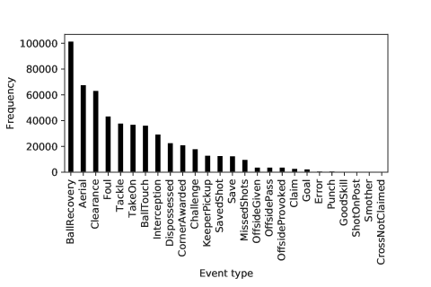
Figure 1: Frequency of each event type observed in the 2013/2014 and 2014/2015 English Premier League seasons. The event type Pass is removed for clarity as it occurs with a ratio of approximately 10:1 over BallRecovery.

In determining a player’s ability for a given event type we make the assumption that the more times a player is involved the better they are at that event type. For example, a player who makes more passes than another player is assumed to be the better passer. On this basis, we can transform the data to represent the number of each event type each player is involved in at a game by game level. This count data is illustrated in Table 2. It is to this data which the methods of Section 3 will be applied.

Table 2: A section of the count data.

			Count for each event type
game id	player id	team id	Goal	Pass	Tackle	$\cdots$
1483412	17	663	0	97	3
1483412	3817	663	0	37	3
1483412	4574	663	0	73	3
⋮	⋮	⋮	⋮	⋮	⋮
1483831	10136	676	1	36	4
1483831	12267	676	0	45	0
1483831	12378	676	0	52	2
⋮	⋮	⋮	⋮	⋮	⋮

3 Model

Consider the case where we have $K$ matches, numbered $k=1,\ldots,K$. We denote the set of teams in game $k$ as $T_{k}$, with $T_{k}^{H}$ and $T_{k}^{A}$ representing the home and away teams respectively. Hence, $T_{k}=\{T_{k}^{H},T_{k}^{A}\}$. We take $P$ to be the set of all players who feature in the dataset, and $P_{k}^{j}\subset P$ to be the subset of players who play for team $j$ in game $k$. We may want to consider how players’ abilities over different event types interact. For this, we group event types to create meaningful interactions. In grouping events there is an underlying assumption about the independence between the events that make up a grouped event. To the authors knowledge there is no evidence in the existing literature of interactions which are clearly detectable from data (a question we believe would make a very interesting area of future research). For simplicity, we describe the model for a single pair of event types which are deemed to interact, for example, Pass and Interception, and we denote these event types $e_{1}$ and $e_{2}$, with $E=\{e_{1},e_{2}\}$.

Taking $X_{i,k}^{e}$ as the number of occurrences (counts) of event type $e$, by player $i$ (who plays for team $j$), in match $k$, we assume that

$$X_{i,k}^{e}\sim Poisson\left(\eta_{i,k}^{e}\tau_{i,k}\right),$$ (1)

where

$$\eta_{i,k}^{e}=\exp\left\{\Delta_{i}^{e}+\tau_{i,k}\left(\lambda_{1}^{e}\sum_{i^{\prime}\in P_{k}^{j}}\Delta_{i^{\prime}}^{e}-\lambda_{2}^{e}\sum_{i^{\prime}\in P_{k}^{T_{k}\setminus j}}\Delta_{i^{\prime}}^{E\setminus e}\right)+\left(\delta_{T_{k}^{H},j}\right)\gamma^{\,e}\right\},$$ (2)

$\delta_{r,s}$ is the Kronecker delta and $\tau_{i,k}$ is the fraction of time player $i$ (playing for team $j$) spent on the pitch in match $k$, with $\tau_{i,k}\in[0,1]$. Specifically, if a player plays 60 minutes of a 90 minute match then $\tau_{i,k}=2/3$. The home effect is represented by $\gamma^{\,e}$. The home effect reflects the (supposed) advantage the home team has over the away team in event type $e$. The $\Delta_{i}^{e}$ represent the (latent) ability of each player for a specific event type, where we let $\Delta$ be the vector of all players abilities. The impact of a player’s own team on the number of occurrences is captured through $\lambda_{1}^{e}$, with $\lambda_{2}^{e}$ describing the opposition’s ability to stop the player in that event type. Whilst the inclusion of $\tau_{i,k}$ in (1) is obvious, its inclusion in (2) is more nuanced. Here, across different games with the same player, we aim to capture variability in rate $\eta_{i,k}^{e}$ as team strategy varies from game to game: a change of time played by player $i$ explains other unobserved features of the game meant to affect rate $\eta_{i,k}^{e}$ directly. A version of (2) was initially considered where a player would have their own individual parameter governing their ability to interact with their team in an event type and how put off they would be by the opposition. We found that this led to a model with too many parameters for succinct consideration and fitting. Expert football analysts suggested that a time a player played in a given game would act as a good proxy in the absence of a specific parameter. The inclusion of $\tau_{i,k}$ in (2) is discussed further in Section 4.1. As $\tau_{i,k}\in[0,1]$ a player therefore receives a proportion of their own teams ability (and opposition’s ability to stop) determined by the time they play in a given game. For identifiability purposes, we impose the constraint that the $\lambda$s must be positive. Figure 2 illustrates the model for one game, allowing for some abuse in notation, and where we assume each team consists of 11 players only (that is, we ignore substitutions) and suppress the time dependence ($\tau$). From (1) and (2), the log-likelihood is given by

$$\ell=\sum_{e\in E}\sum_{k=1}^{K}\sum_{j\in T_{k}}\sum_{i\in P_{k}^{j}}X_{i,k}^{e}\log{\left(\eta_{i,k}^{e}\tau_{i,k}\right)}-\eta_{i,k}^{e}\tau_{i,k}-\log{\left(X_{i,k}^{e}\,!\right)}.$$ (3)

Figure 2: Pictorial representation of the model for one game. For ease we assume that only 11 players play for each team (that is, we ignore substitutions) and suppress the time dependence ($\tau$).

Interest lies in estimating this model using a Bayesian approach. We put independent Gaussian priors over all abilities, whilst treating the remaining unknown parameters as hyperparameters to be fitted by the marginal likelihood function. Given the size of the data and the number of parameters needing to be estimated to fit equation (3) we appeal to variational inference techniques, which are the subject of the next section.

3.1 Variational inference

In contrast to some other techniques for Bayesian inference, such as MCMC, in variational inference (VI) we specify a variational family of densities over latent variables. We introduce the basic idea with a general notation, using $x$ to denote observed data and $\nu$ the set of latent variables, here assumed to be continuous. In VI we aim to find the best candidate approximation, $q^{*}(\nu)$, to minimise the Kullback-Leibler (KL) divergence to the posterior $\pi(\nu|x)$ within a suitable space $\mathcal{Q}$ of density functions

$$q^{*}(\nu)=\underset{q\left(\nu\right)\in\mathcal{Q}}{\textrm{argmin KL}}\left\{q(\nu)||\pi(\nu|x)\right\}.$$

Unfortunately, due to the analytic intractability of the posterior distribution the KL divergence is not available in closed (analytic) form. However, it is possible to maximise the evidence lower bound (ELBO). The ELBO is the expectation of the joint density under the approximation plus the entropy of the variational density and is given by

$$\textrm{ELBO}\left\{q\left(\nu\right)\right\}=\textrm{E}_{q\left(\nu\right)}\left[\log\left\{\pi\left(\nu,x\right)\right\}\right]-\textrm{E}_{q\left(\nu\right)}\left[\log\left\{q\left(\nu\right)\right\}\right].$$ (4)

The ELBO is the equivalent of the negative KL divergence up to the constant $\log\{\pi(x)\}$, and from Jordan et al., (1999) and Bishop, (2006) we know that by maximising the ELBO we minimise the KL divergence.

In performing VI, assumptions must be made about the variational family $\mathcal{Q}$ to which $q(\nu)$ belongs. Here we consider the mean-field variational family, in which the latent variables are assumed to be mutually independent. Moreover, each latent variable $\nu_{r}$ is governed by its own variational parameters $\phi_{r}$. They determine $\nu_{r}$’s variational factor, the density $q(\nu_{r}|\phi_{r})$. Specifically, for $R$ latent variables, we have that

$$q\left(\nu\right)=\prod_{r=1}^{R}q\left(\nu_{r}|\phi_{r}\right).$$ (5)

We note that the complexity of the variational family determines the complexity of the optimisation, and hence impacts the computational cost of any VI approach. In general, it is possible to impose any graphical structure on $q(\nu)$; a fully general graphical approach leads to structured variational inference, see Saul and Jordan, (1996). Furthermore, the data ($x$) does not feature in equation (5), meaning the variational family is not a model of the observed data. It is in fact the ELBO which connects the variational density, $q(\nu)$, to the data and the model.

For the model outlined at the beginning of this section, let $\nu=\Delta$, and set

$$q\left(\Delta_{i}^{e}|\phi_{i}^{e}\right)\sim N\left(\mu_{\Delta_{i}^{e}},\sigma_{\Delta_{i}^{e}}^{2}\right).$$ (6)

Our aim is to find suitable candidate values for the variational parameters

$$\phi_{i}^{e}=\left(\mu_{\Delta_{i}^{e}},\sigma_{\Delta_{i}^{e}}\right)^{\prime},\qquad\forall i,\forall e,$$

where ^′ denotes the transpose. We take

$$q\left(\Delta\right)=\prod_{e\in E}\prod_{j\in T}\prod_{i\in P^{j}}q\left(\Delta_{i}^{e}|\phi_{i}^{e}\right),$$ (7)

where $T$ is the set of all teams and $P^{j}$ are the players who play for team $j$. Finally we take $\psi=~{}(\lambda_{1}^{e_{1}},\lambda_{2}^{e_{1}},\gamma^{\,e_{1}},\lambda_{1}^{e_{2}},\lambda_{2}^{e_{2}},\gamma^{\,e_{2}})^{\prime}$ to be fixed parameters, and assume each $\Delta_{i}^{e}$ follows a $N(m,s^{2})$ prior distribution, fully specifying the model given by equations (1)–(3). Thus, the ELBO (4) is given by

$$\textrm{ELBO}\left\{q\left(\Delta\right)\right\} =\sum_{e\in E}\sum_{k=1}^{K}\sum_{j\in T_{k}}\sum_{i\in P_{k}^{j}}\textrm{E}_{q\left(\Delta_{i}^{e}\right)}\left[\log\left\{\pi\left(\Delta_{i}^{e},\phi_{i}^{e},\psi,x\right)\right\}\right]-\textrm{E}_{q\left(\Delta_{i}^{e}\right)}\left[\log\left\{q\left(\Delta_{i}^{e}|\phi_{i}^{e}\right)\right\}\right]$$

$$=\sum_{e\in E}\sum_{k=1}^{K}\sum_{j\in T_{k}}\sum_{i\in P_{k}^{j}}\textrm{E}_{q\left(\Delta_{i}^{e}\right)}\left[\log\left\{\pi\left(\Delta_{i}^{e}\right)\right\}\right]+\textrm{E}_{q\left(\Delta_{i}^{e}\right)}\left[\log\left\{\pi\left(x|\Delta_{i}^{e},\phi_{i}^{e},\psi\right)\right\}\right]$$

$$\qquad\qquad\qquad\qquad\quad-\textrm{E}_{q\left(\Delta_{i}^{e}\right)}\left[\log\left\{q\left(\Delta_{i}^{e}|\phi_{i}^{e}\right)\right\}\right].$$ (8)

The above is available in closed-form (see Appendix A for the explicit expressions). Whilst in classical VI optimisation is done by coordinate ascent, where the optimal solution for each $\phi_{i}^{e}$ can be found in closed form by fixing all other free parameters, it is widely accepted today that generic gradient-based optimisers are better suited. In particular, with the popularisation of automatic differentiation tools such as the Python package autograd (Maclaurin et al.,, 2015), programming requirements are minimal: it suffices to implement only (8), as given in Appendix A, and pass this function call to a gradient-based optimisation library that can internally make use of a tool such as autograd. Whilst libraries such as the Automatic Differentiation Variational Inference (ADVI) engine by Kucukelbir et al., (2017) are available, they are particularly useful when the ELBO cannot be computed analytically. In our case, we found it easier to implement (8) in native Python along with a call to a standard optimiser (ADAM) coupled with autograd.

3.2 Hierarchical model

Building on the methods of Section 3.1, we wish to discover whether the inferred $\Delta$s have any impact on our ability to predict the goals scored in a football match. This provides an indirect and objective validation that our estimated latent abilities are capturing information concerning a player’s performance. As a baseline model we consider the work of Baio and Blangiardo, (2010), who present the model of Karlis and Ntzoufras, (2003) in a Bayesian framework. The model has close ties with the models in Dixon and Coles, (1997), Lee, (1997) and Karlis and Ntzoufras, (2000), which have all previously been used to predict football scores. We first briefly outline the model of Baio and Blangiardo, (2010) before offering our extension to include the imputed $\Delta$s.

The model is a Poisson-log normal model; see for example Aitchison and Ho, (1989), Chib and Winkelmann, (2001) and Tunaru, (2002) (amongst others). For a particular game $k$ we let $y^{k}=~{}(y^{k}_{h},y^{k}_{a})^{\prime}$ be the total number of goals scored, where $y^{k}_{h}$ is the number of goals scored by the home team, and $y^{k}_{a}$ the number by the away team. Inherently, we let $h$ denote the home team and $a$ the away team for the given game $k$. The goals of each team are modelled by independent Poisson distributions, such that

$$y_{t}^{k}|\theta_{t}\overset{indep}{\sim}Poisson\left(\theta_{t}\right),\qquad t\in\{h,a\},$$ (9)

where

$$\log{\left(\theta_{h}\right)} =\textrm{home}+\textrm{att}_{h}+\textrm{def}_{a},$$ (10)

$$\log{\left(\theta_{a}\right)} =\textrm{att}_{a}+\textrm{def}_{h}.$$ (11)

Each team has their own team-specific attack and defence ability, att and def respectively, which form the scoring intensities $(\theta_{t})$ of the home and away teams. A home effect $(\textrm{home})$, which is assumed to be constant across all teams and across the time-span of the data is also included in the rate of the home team’s goals.

For identifiability we follow Baio and Blangiardo, (2010) and Karlis and Ntzoufras, (2003), and impose sum to zero constraints on the attack and defence parameters

$$\sum_{t\in T}\textrm{att}_{t}=0\qquad\textrm{and}\qquad\sum_{t\in T}\textrm{def}_{t}=0,$$

where $T$ is the set of all teams to feature in the dataset. Furthermore, the attack and defence parameters for each team are seen to be draws from a common distribution

$$\textrm{att}_{t}\sim N\left(\mu_{\textrm{att}},\sigma_{\textrm{att}}^{2}\right)\qquad\textrm{and}\qquad\textrm{def}_{t}\sim N\left(\mu_{\textrm{def}},\sigma_{\textrm{def}}^{2}\right).$$

We follow the prior setup of Baio and Blangiardo, (2010) and assume that home follows a $N(0,100^{2})$ distribution a priori, with the hyper parameters having the priors

$$\mu_{\textrm{att}}\sim N\left(0,100^{2}\right), \qquad\mu_{\textrm{def}}\sim N\left(0,100^{2}\right),$$

$$\sigma_{\textrm{att}}\sim Inv\textrm{-}Gamma(0.1,0.1), \qquad\sigma_{\textrm{def}}\sim Inv\textrm{-}Gamma(0.1,0.1).$$

A graphical representation of the model is given in Figure 3.

Figure 3: Pictorial representation of the Bayesian hierarchical model. Removing both $f(q(\Delta))_{h}$ and $f(q(\Delta))_{a}$ gives the baseline model of Baio and Blangiardo, (2010).

As an extension to the model of Baio and Blangiardo, (2010) we propose to include information about the distribution of the latent $\Delta$s of Section 3.1 in the scoring intensities of both the home and away teams. Explicitly (10) and (11) become

$$\log{\left(\theta_{h}\right)} =\textrm{home}+\textrm{att}_{h}+\textrm{def}_{a}+f\left(q(\Delta)\right)_{h},$$ (12)

$$\log{\left(\theta_{a}\right)} =\textrm{att}_{a}+\textrm{def}_{h}+f\left(q(\Delta)\right)_{a},$$ (13)

where $f(q(\Delta))$ is to be determined. For a single pair of event types (as outlined at the start of this section), our choice for $f(q(\Delta))$ in this paper is

$$f\left(q(\Delta)\right)_{h} =\sum_{i\in I_{k}^{T_{k}^{H}}}\mu_{\Delta_{i}^{e}}-\sum_{i\in I_{k}^{T_{k}^{A}}}\mu_{\Delta_{i}^{E\setminus e}}$$ (14)

and

$$f\left(q(\Delta)\right)_{a} =\sum_{i\in I_{k}^{T_{k}^{A}}}\mu_{\Delta_{i}^{e}}-\sum_{i\in I_{k}^{T_{k}^{H}}}\mu_{\Delta_{i}^{E\setminus e}},$$ (15)

with $I_{k}^{j}$ being the initial eleven players who start game $k$ for team $j$, and $\mu_{\Delta}$ being the mean of the marginal posterior variational densities. This extension is also illustrated in Figure 3. Through our empirical investigations we found little difference between trying different event types one by one or where $f(q(\Delta))$ is a summation over event types. Therefore, for ease, from this point forward we only consider the case in which $f(q(\Delta))$ is a summation over event types. The question around which specific event types should enter this summation is considered in Section 4.2.

We fit both the baseline model of Baio and Blangiardo, (2010) and our extension using PyStan (Stan Development Team,, 2016).

4 Applications

Having outlined our approach to determine a player’s ability in a given event type, and offered an extension to the model of Baio and Blangiardo, (2010) to capture the goals scored in a specific game, we wish to test the proposed methods in real world scenarios. We therefore consider two applications. In the first we use data from the 2013/2014 English Premier League to learn players abilities across the season as a whole for a number of event types, including the ability to score a goal. The second example concerns the number of goals observed in a given game, specifically we predict whether a certain number of goals will be scored (or not) in each game, offering validation against the betting market.

4.1 Determining a player’s ability

In this section we consider the touch-by-touch data described in Section 2 and consider data for the 2013/2014 English Premier League season only. We look to create an ordering of players abilities, from which we hope to extract meaning based on what we know of the season. We also have data on the amount of time each player spent on the pitch in each match and this information is factored in accordingly through $\tau_{i,k}$. The season consisted of 380 matches for the 20 team league, with 544 different players used during matches. The final league table is shown in Table 3. From this table, we note that Manchester City and Liverpool were the teams who scored the most goals, with Chelsea conceding the least. These teams did well over the season and we expect players from these teams to have high abilities. The teams to do worst (and got relegated), were Norwich City, Fulham and Cardiff; we do not expect players from these teams to feature highly in any ordering created. A final note is that, in this season Manchester United underperformed (given past seasons) under new manager David Moyes. Whence, $k=1,\ldots,380$, $j\in T_{k}$ where $T_{k}$ consists of a subset of $\{1,\ldots,20\}$ and $i\in P_{k}^{j}$ where $P_{k}^{j}$ is a subset of $P=\{1,\ldots,544\}$.

Table 3: Final league table for the 2013/2014 English Premier League. Pl matches played, W matches won, D matches drawn, L matches lost, F goals scored, A goals conceded, GD goal difference ($\textrm{scored}-\textrm{conceded}$), Pts final points total.

2013/2014 English Premier League
Pos	Team	Pl	W	D	L	F	A	GD	Pts
1	Manchester City	38	27	5	6	102	37	65	86
2	Liverpool	38	26	6	6	101	50	51	84
3	Chelsea	38	25	7	6	71	27	44	82
4	Arsenal	38	24	7	7	68	41	27	79
5	Everton	38	21	9	8	61	39	22	72
6	Tottenham Hotspur	38	21	6	11	55	51	4	69
7	Manchester United	38	19	7	12	64	43	21	64
8	Southampton	38	15	11	12	54	46	8	56
9	Stoke City	38	13	11	14	45	52	-7	50
10	Newcastle United	38	15	4	19	43	59	-16	49
11	Crystal Palace	38	13	6	19	33	48	-15	45
12	Swansea City	38	11	9	18	54	54	0	42
13	West Ham United	38	11	7	20	40	51	-11	40
14	Sunderland	38	10	8	20	41	60	-19	38
15	Aston Villa	38	10	8	20	39	61	-22	38
16	Hull City	38	10	7	21	38	53	-15	37
17	West Bromwich Albion	38	7	15	16	43	59	-16	36
18	Norwich City	38	8	9	21	28	62	-34	33
19	Fulham	38	9	5	24	40	85	-45	32
20	Cardiff City	38	7	9	22	32	74	-42	30

For a pair of interacting event types we fit the model defined by (1)–(3), by maximising (8) where $q(\cdot)$ follows (6). This model setup has 2182 parameters $[544\times(\mu_{\Delta_{i}^{e_{1}}},\mu_{\Delta_{i}^{e_{2}}},\sigma_{\Delta_{i}^{e_{1}}},\sigma_{\Delta_{i}^{e_{2}}})+\lambda_{1}^{e_{1}}+\lambda_{2}^{e_{1}}+\gamma^{\,e_{1}}+\lambda_{1}^{e_{2}}+\lambda_{2}^{e_{2}}+\gamma^{\,e_{2}}]$ governing any two interacting event types. We take a reasonably uninformative prior

$$\pi\left(\Delta_{i}^{e}\right)\sim N\left(-2,2^{2}\right),$$ (16)

where $-2$ represents the ability of an average player. We found little difference in results for alternative priors. We begin by considering occurrences of Goal and GoalStop. GoalStop is an event type of our own creation (in conjunction with expert football analysts at Stratagem Technologies), made up of many other event types (BallRecovery, Challenge, Claim, Error, Interception, KeeperPickup, Punch, Save, Smother, Tackle), with BallRecovery being the event type where a player collects the ball after it has gone loose. GoalStop aims to represent all the things a team can do to stop the other team from scoring a goal. A Monte Carlo simulation of the prior for $\eta_{i,k}^{\textrm{Goal}}$ using 100K draws of $\Delta_{i}^{\textrm{Goal}}$ from (16) is shown in Figure 4, where most players are viewed to score 0 or 1 goal (as expected).

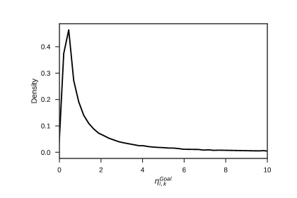
Figure 4: Monte Carlo simulation of the prior for $\eta_{i,k}^{\textrm{Goal}}$ using 100K draws of $\Delta_{i}^{\textrm{Goal}}$ from (16).

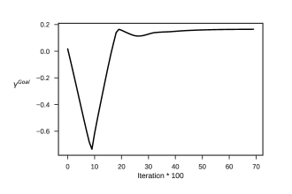
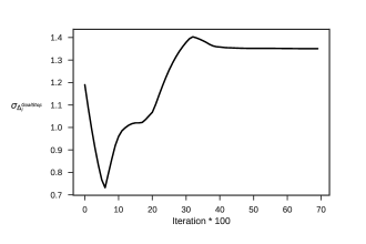
Figure 5: Trace plots for the ELBO and a selection of the model parameters outputted every 100 iterations.

We ran the model for 7000 iterations to achieve convergence. Trace plots of the ELBO and a selection of model parameters are shown in Figure 5. It is clear that convergence has been achieved (measured via the ELBO). For completeness the values of the fixed parameters ($\psi$) under the model are given in Table 4, where all respective parameters appear to be on the same scale. We observe small differences in the parameters dictating the amount of impact both a player’s own team, and the opposing team has on occurrences of an event type. There are more noticeable differences in the home effects of each event type, with the home effect for Goal being much larger than that of GoalStop. This is in line with other research around the goals scored in a match, where a clear home effect is acknowledged; see Dixon and Coles, (1997), Karlis and Ntzoufras, (2003) and Baio and Blangiardo, (2010) for further discussion of this home effect. The home effect for GoalStop is closer to zero, suggesting the number of attempts a team makes to stop a goal is similar whether they are playing at home or away.

Figure 6 shows the $\eta_{i,k}^{e}$ (2) we obtain when the model parameters are combined for 2 randomly selected matches, where we set $\Delta_{i}^{e}$ to be $\mu_{\Delta_{i}^{e}}$. We plot these against the observed counts and include the 95% prediction intervals for each $\eta_{i,k}^{e}$ to add further clarity. The solid line on each plot separates the players from the two opposing teams. A large number of the model $\eta$s are close to the observed counts (especially for GoalStop), and nearly all observed values fall within the 95% prediction intervals. The number of goal-stops across teams is not particularly variable, however there is some evidence of player variability (although this is somewhat clouded by the fact that substitutes are not specifically marked in the figure, as we would expect them to register lower counts by virtue of less playing time).

Goal

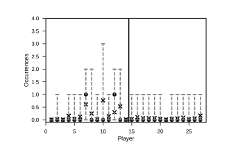
GoalStop

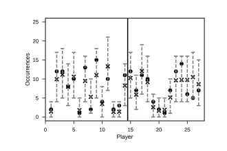
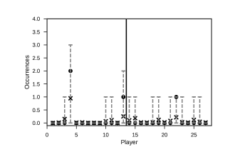
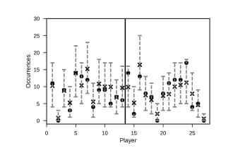
Figure 6: Within sample predictive distributions for the number of goals/goal-stops in 2 randomly selected matches. Cross model combinations of $\eta_{i,k}^{e}$, circle observed counts, dashed bars 95% prediction interval for each $\eta_{i,k}^{e}$. The solid line separates the players from the two teams. The teams involved in the matches are Cardiff City, Hull City, Liverpool and Manchester City.

We sample the marginal posterior variational densities, $q(\Delta_{i}^{e})$, 10K times (constructing the corresponding $\eta_{i,k}^{e}$) and simulate from the relevant Poisson distributions (with mean $\eta_{i,k}^{e}\tau_{i,k}$). This gives a Monte Carlo simulation of each player’s number of goals and goal-stops for each game in the 2013/2014 English Premier League. Summing over the players who played in a given match gives a within sample prediction of the total number of goals/goal-stops for each team in every game. We present the predictive distributions of these totals for GoalStop in Figure 7, where for reference we also include histograms for each team’s total number of goal-stops in each game constructed from the touch-by-touch data. The model is clearly capturing the patterns between differing teams (and the patterns observable within the data). We note, slightly surprisingly, that there appears to be no connection between the occurrences of GoalStop and the goals a team concedes, with both Chelsea and Norwich City having similar predictive distributions despite conceding a vastly different number of goals, 27 and 62 respectively. There is some suggestion that such observations may be used to determine a team’s style of play, for example, whether they are a passing team or follow the long ball philosophy. We leave such questions for future investigation given the setup we derive here. We can conclude, nevertheless, that the model is capturing the trends observed in the touch-by-touch data well.

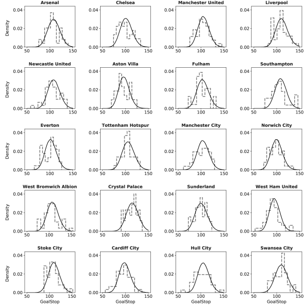
Figure 7: Within sample predictive distributions for the total number of goal-stops in a game for each team in the 2013/2014 English Premier League solid. The observed totals from the 38 games is given by the histograms dashed.

Marginal posterior variational densities of Goal, $q(\Delta_{i}^{\textrm{Goal}})$, for two players are presented in Figure 8, where $q(\Delta_{i}^{\textrm{Goal}})$ takes the form of (6) and the prior is (16). The two players shown are Daniel Sturridge and Harrison Reed. Sturridge played 29 times over the season totalling 2414 minutes of match time, scoring 21 goals, whereas Reed played 4 times totalling 23 minutes, scoring zero goals. These attributes are clearly captured by the posteriors; the greater number of observations for Sturridge leading to a posterior with a much smaller variance. The high number of goals scored by Sturridge leads to him having a higher value of $\mu_{\Delta_{i}^{\textrm{Goal}}}$ (with reasonable certainty), whilst the lack of both goals and playing time leads to a posterior for Reed which resembles the prior.

Table 4: Values of the fixed parameters ($\psi$) for interacting event types Goal and GoalStop.

	Fixed parameter
Event type ($e$)	$\lambda_{1}^{e}$	$\lambda_{2}^{e}$	$\gamma^{e}$
Goal	$2.907\times 10^{-8}$	0.041	0.165
GoalStop	$1.621\times 10^{-7}$	0.009	0.003

Sturridge

Reed

Figure 8: Marginal posterior variational densities of Goal for 2 players in the 2013/2014 English Premier League. Dashed prior, solid posterior.

The model is capturing differences between players abilities, as evidenced by the posteriors of Figure 8. Thus, the natural question to ask is whether these differences are sensible, and, if we were to order the players by their inferred ability, would this ordering agree with (a debatable) reality. Hence, we construct the marginal posterior variational densities for all players and rank them according to the 2.5% quantile of these densities. A top 10 for Goal is presented in Table 5, with a ranking for GoalStop given in Table 6. We present top 10 lists for other event types in Appendix B. The ranking shown in Table 5 appears sensible and comprises of those players who were the main goal scorers (strikers) for the best teams, and the players who scored nearly all the goals a lesser team scored over the season. The ranking is very close to that obtained by ranking players on the total number of goals scored over the season (although there is some debate in the football community as to whether this is a sensible way of ranking, with some suggesting a ranking based on a per 90 minute statistic, however this can be distorted by those with very little playing time, see Chapter 3 of Anderson and Sally, (2013) or AGR Analytics, (2016) for further discussion). The questionable deviations from this ranking are Aguero (ranked third) and van Persie (ranked seventh). Both these players have less playing time over the season compared to their competitors, and thus, the model highlights them as better goal scorers, given the time available to them, than other players based on total goals scored. Expert football analysts agreed with this view when we showed them these rankings. Suarez has an inferred ability much greater than any other player, which is evidenced by the 31 goals he scored (10 more than any other player). At points the difference between successive ranks is small, suggesting some players are harder to distinguish between. Finally, we note that the standard deviations for all players in the top 10 are roughly the same, meaning we have similar confidence in the ability of any of these players.

Table 5: Top 10 goal scorers in the 2013/2014 English Premier League based on the 2.5% quantile of the marginal posterior variational density for each player, $q(\Delta_{i}^{\textrm{Goal}})$.

Goal - top 10
Rank	Player	Team	2.5%	Mean	Standard	Observed	Observed	Rank	Time
			quantile		deviation		rank	difference	played
1	Suarez	Liverpool	0.508	0.869	0.184	31	1	0	3185
2	Sturridge	Liverpool	0.176	0.617	0.225	21	2	0	2414
3	Aguero	Manchester City	0.147	0.636	0.250	17	4	+1	1616
4	Y. Toure	Manchester City	-0.043	0.395	0.224	20	3	-1	3113
5	Rooney	Manchester United	-0.056	0.421	0.243	17	5	0	2625
6	Dzeko	Manchester City	-0.065	0.424	0.249	16	8	+2	2128
7	van Persie	Manchester United	-0.136	0.430	0.289	12	15	+8	1690
8	Remy	Newcastle United	-0.230	0.302	0.271	14	11	+3	2274
9	Bony	Swansea City	-0.257	0.238	0.252	16	7	-2	2644
10	Rodriguez	Southampton	-0.354	0.161	0.263	15	10	0	2758

The ranking of GoalStop (Table 6) appears at first glance to be less sensible than that of Table 5. It features 3 players with comparatively larger standard deviations, Kallstrom (rank 2), Lewis (rank 6) and Palacios (rank 7). Whilst these players did well with the little playing time afforded to them, it is somewhat presumptuous to postulate that they would maintain a similar level of ability given more game time, leading to their ranking slipping. Ideally we would provide several tables for each event type, filtering players by the amount of uncertainty surrounding them, although such an approach would be unwieldy given the large number of players in the dataset. Moreover, fully factorised mean-field approximations are known to underestimate the uncertainty of the posterior (Bishop,, 2006). Although comparative uncertainty between players is easier to gauge, it is less clear how to quantify how much bias is being added to the variances of each latent variable individually. In a future work this could be mitigated by adopting a variational approximation that accounts for some correlations of the latent variables, or by correcting for the variances using the approach of Giordano et al., (2018). However, the rest of the list appears sensible and is made up mainly of defensive midfielders (whose main role it is to disrupt the oppositions play); only Mannone and Ruddy are goalkeepers (discounting the 3 players with large standard deviations). This suggests, anecdotally given our definition of GoalStop, that to stop a goal it is more prudent to invest in a better defensive midfielder than it is a goalkeeper, presuming you can not just buy the best player in each position. Here, the differences between successive ranks are much smaller than in Table 5, implying it is harder to distinguish between player ability to perform goal-stops than it is the ability to score goals.

Table 6: Top 10 goal-stoppers in the 2013/2014 English Premier League based on the 2.5% quantile of the marginal posterior variational density for each player, $q(\Delta_{i}^{\textrm{GoalStop}})$.

GoalStop - top 10
Rank	Player	Team	2.5%	Mean	Standard	Observed	Observed	Rank	Time
			quantile		deviation		rank	difference	played
1	Mulumbu	West Bromwich Albion	2.575	2.653	0.040	631	1	0	3319
2	Kallstrom	Arsenal	2.553	2.900	0.177	33	405	+403	144
3	Mannone	Sunderland	2.528	2.615	0.044	508	12	+9	2767
4	Yacob	West Bromwich Albion	2.510	2.614	0.053	359	43	+39	1979
5	Tiote	Newcastle United	2.474	2.560	0.044	517	8	+3	2988
6	Lewis	Cardiff City	2.446	2.863	0.213	23	436	+430	98
7	Palacios	Stoke City	2.441	2.638	0.101	100	286	+279	585
8	Jedinak	Crystal Palace	2.420	2.500	0.041	603	2	-6	3651
9	Ruddy	Norwich City	2.411	2.491	0.041	600	3	-6	3679
10	Arteta	Arsenal	2.409	2.503	0.048	431	21	+11	2615

Overall, the model provides a good fit to the data and suggests a reasonable prowess to determine a player’s ability in a specific event type, with marginal posterior variational densities providing a good visual comparison between different players abilities (and the confidence surrounding that ability).

Sensitivity analysis for the contribution of $\tau_{i,k}$

To address questions remaining about the inclusion of $\tau_{i,k}$ in (2), we investigate the validity of this decision by considering the predictive performance of  (2) versus a simplified version of (2) where $\tau_{i,k}$ is suppressed. We test both versions of the model on the scenario described in Section 4.1. Calculating out-of-sample prediction biases for the events Goal, GoalStop and Shots we found that the model described in this paper gave 0.201, 4.374 and 0.807 respectively, with 0.237, 5.130, 0.807 observed for the model without $\tau_{i,k}$. We see an improved prediction bias for Goal and GoalStop when the model includes $\tau_{i,k}$ with the same result seen under both models for Shots. As our ultimate aim within this paper lies with prediction, we therefore favour the model including time described by (1) and (2). The inclusion of time is not an obvious one, and whilst it improves prediction, that on it’s own is not reason enough. We believe by acting as a proxy for how much a player interacts with their team in an event type and how put off they would be by the opposition, it may also capture some of the more nuanced aspects of a football game, for example, a player’s importance in a manager’s formation. Capturing the many nuances affecting a player in a football game would be an interesting area for future research, although given the near endless possibilities up for inclusion, the form of the model used in this paper may be restrictive. In the next section we look to utilise the player abilities explored in Section 4.1 in the prediction of goals in a football match.

4.2 Prediction

A key betting market stemming from the rise of online betting is the over/under market (Betfair,, 2017; betHQ,, 2017; SPORTINGINDEX,, 2017), where people bet on whether over or under 2.5 goals will be scored in a match. Here we attempt to predict whether 2.5 goals will be scored or not in a given game. To predict the goals scored in a game which takes place in the future we first fit the model on all the past available to us. We use a whole season of data to train the model, before predicting the following season in incremental blocks. Here, we use the entirety of the 2013/2014 English Premier League season (380 games) to train the model, before attempting to predict the goals scored in each match of the 2014/2015 English Premier League season. The reason why we use the whole of the 2013/2014 season to train the model, and only predict on the 2014/2015 season, is that the odds data available to us only covers the 2014/2015 season. We introduce the games (on which we predict) in blocks of size 80, with a final block of 60 games to total 380 (the number of games over a season). In each case we use all of the available past to fit the model, that is, in predicting the second block of 80 games in the 2014/2015 season, we use all of the 2013/2014 season and the first block of the 2014/2015 season to fit the model. Figure 9 shows a graphical representation of this approach.

Figure 9: Illustration of the approach to prediction. The model is fit on all past data before predictions are made for a future block of games. Solid fit, dashed predict.

For the extension to the model of Baio and Blangiardo, (2010) (which we consider to be the baseline model), we include the latent player abilities for the event types Goal, Shots and ChainEvents, with their counterparts being GoalStop, ShotStop and AntiPass respectively. Goal and GoalStop are as defined in Section 4.1, whilst Shots and ShotStop have homogeneous roots to Goal and GoalStop, that being the ability to shoot or to stop a shot. ChainEvents represents how prevalent a player is in the lead up to a good attacking chance, with AntiPass being a player’s ability to stop the other team from passing the ball. We refer the reader to Appendix B for the more technical definitions of these event types. Explicitly (14) and (15) are given by

$$f\left(\Delta\right)_{h} =\sum_{i\in I_{k}^{T_{k}^{H}}}\left(\Delta_{i}^{\textrm{Goal}}+\Delta_{i}^{\textrm{Shots}}+\Delta_{i}^{\textrm{ChainEvents}}\right)$$

$$\qquad\qquad-\sum_{i\in I_{k}^{T_{k}^{A}}}\left(\Delta_{i}^{\textrm{GoalStop}}+\Delta_{i}^{\textrm{ShotStop}}+\Delta_{i}^{\textrm{AntiPass}}\right)$$ (17)

and

$$f\left(\Delta\right)_{a} =\sum_{i\in I_{k}^{T_{k}^{A}}}\left(\Delta_{i}^{\textrm{Goal}}+\Delta_{i}^{\textrm{Shots}}+\Delta_{i}^{\textrm{ChainEvents}}\right)$$

$$\qquad\qquad-\sum_{i\in I_{k}^{T_{k}^{H}}}\left(\Delta_{i}^{\textrm{GoalStop}}+\Delta_{i}^{\textrm{ShotStop}}+\Delta_{i}^{\textrm{AntiPass}}\right),$$ (18)

where $I_{k}^{j}$ is the initial eleven players who start game $k$ for team $j$. We also considered including a player’s ability to pass, but found this led to no increase in predictive power (and in some instances diminished it). We found little difference when setting $\Delta_{i}^{e}$ to be either $\mu_{\Delta_{i}^{e}}$ or the 2.5% quantile of $q(\Delta_{i}^{e})$ in (17) and (18), and so here report results for the mean ($\mu_{\Delta_{i}^{e}}$).

Both the models were fit using PyStan and were run long enough to yield a sample of approximately 10K independent posterior draws, after an initial burn in period. The teams which feature in the data are those in Table 3, with the addition of Burnley, Leicester City and Queens Park Rangers who replaced the relegated teams of Cardiff City, Fulham and Norwich City for the 2014/2015 season. The setup outlined at the beginning of this section allows us to view the evolution of a team’s attack/defence parameter or a player’s latent ability through time after different fitting blocks. We denote block 0 to be all the games in the 2013/2014 English Premier League season, block 1 to be block 0 plus the first 80 games of the 2014/2015 season, block 2 to be block 1 plus the next 80 games, block 3 to include the next 80 games, with block 4 including the next 80 games again. As an indication, for block 1, the mean predictive log-likelihood for the model including the latent player abilities is $-163.106$ with the baseline model having a mean predictive log-likelihood of $-159.578$ (this is the log-likelihood of the second 80 games of the 2014/2015 season having fit the models using data in block 1). We observe similar results across all other blocks. However, we believe the main judgement of the models within the context of this paper will be the quality of the predictions they produce and not solely the log-likelihood.

Baseline

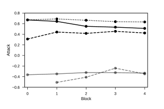
Including latent player abilities

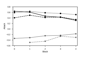
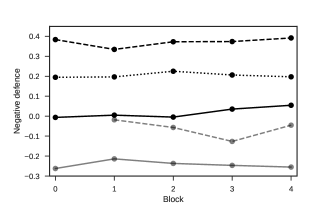
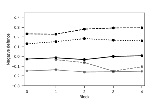
Figure 10: Attack and defence parameters through time under the baseline model and the model including the latent player abilities for selected teams. Top row attack, bottom row negative defence. Black-solid Liverpool, black-dashed Chelsea, black-dotted Manchester City, grey-solid Cardiff City, grey-dashed Burnley.

The attack and defence parameters through time for both the baseline model and the model including the latent player abilities for selected teams are shown in Figure 10, where we plot negative defence so that positive values indicate increased ability. Recall that these parameters for all teams must sum to zero. We see similar, but not identical patterns under both models. The model including latent player abilities reduces the variance of the attack and defence parameters compared to the baseline model, suggesting the inclusion of the $\Delta$s accounts for some of a team’s attack and defensive ability. Manchester City and Chelsea follow similar patterns under both models, with Chelsea clearly having the best defence parameter. Including the $\Delta$s impacts Liverpool’s attacking ability, where the removal of Suarez (Liverpool’s best attacking player who transferred to Barcelona between the 2013/2014 and 2014/2015 seasons) clearly reduces Liverpool’s attacking threat at a more drastic rate than the baseline model. This is in line with reality, where Liverpool only scored 52 goals over the 2014/2015 season compared to 101 goals the previous year. Cardiff City, who got relegated after the 2013/2014 season but feature in all blocks despite not being used for prediction (as games involving them can inform the attack and defence abilities of other teams), have relatively constant parameters under both models, accounting for the reduction in variance. Notable for Burnley is the peak/trough observed after block 3; this is due to the fact that Burnley were starting to look at the prospect of relegation and needed to start winning games, hence, they tried (and succeeded) to score more goals in order to win games, but found themselves more likely to concede goals in the process of doing so.

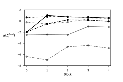
Figure 11: The mean of $q(\Delta_{i}^{\textrm{Goal}})$ through time for a selection of players. Black-solid Costa, black-dashed A. Sanchez, black-dotted Aguero, grey-solid Defoe, grey-dashed G. Johnson, grey-dotted Kane.

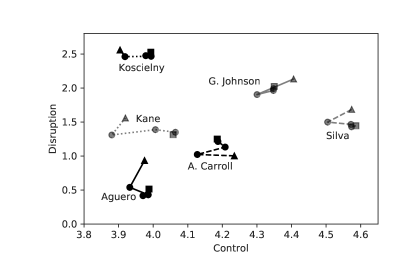
Figure 12: The mean of $q(\Delta_{i}^{\textrm{Control}})$ versus the mean of $q(\Delta_{i}^{\textrm{Disruption}})$ through time for a selection of players. Triangle block 0, square block 4.

The mean of $q(\Delta_{i}^{\textrm{Goal}})$ through time for a selection of players are illustrated in Figure 11. We let this value represent a player’s ability to score a goal. If a player has not featured previously in the data we represent their ability in the figure by the mean of the prior distribution ($-2$). We see that the model is quick to identify a given player’s ability. To elucidate, Costa is immediately (after block 1) identified as one of the top goal scorers despite not featuring in the 2013/2014 season. The same can be said for Sanchez, who takes longer to establish his ability after a less impressive start to the season. Aguero was one of the best goal scorers across all the data and has a constant ability near the top. Kane had little playing time until block 2 where the model starts to increase his ability to score a goal. Defoe spent most of the 2013/2014 season on the bench before transferring to Toronto FC; he returned to the English Premier League with Sunderland in January 2015, where he scored a number of goals, saving Sunderland from relegation. The model rightly acknowledges this and raises his ability as a goal scorer (a trait he is well known for). Given a player scores a small number of goals, relative to other event types, we include G. Johnson to show the effect of scoring a goal. Johnson scored 1 goal in the 2013/2014 and 2014/2015 seasons (during block 2), and his ability rises by a large jump because of this; such jumps are not evident for players who score a reasonable number of goals (5+).

The mean of $q(\Delta_{i}^{\textrm{Control}})$ and the mean of $q(\Delta_{i}^{\textrm{Disruption}})$ are plotted against each other through time for a selection of players in Figure 12. Control and Disruption comprise of the event types listed in Table 1. It is evident that for the majority of players their Control and Disruption abilities do not vary much through time (from block to block). This is perhaps unsurprising given we do not expect a player’s ability to change dramatically from game to game. Those that vary the most are the players with fewer minutes played in the earlier blocks but have much more playing time as time progresses, for example, Kane (see Figure 12). The figure does however show clear distinction between players, with defenders tending to occupy the top half of the graph and strikers the bottom. An interesting extension to this work would be to see whether a clustering analysis of these latent player abilities would reveal player positions, that is, central defender or wing-back for example.

To form our predictions of whether over or under 2.5 goals are scored in a given game, we take each of our posterior draws (fitted using the previous block) and construct the $\theta_{t}$ of (9) via (10) and (11) (baseline model), or (12) and (13) (including latent player abilities) for the games in the following block (our prediction block). Our prediction blocks are formed of games between teams we have already seen in the previous (fitting) blocks, hence prediction block 1 consists of 57 games (as we do not predict on promoted teams in this block), prediction blocks 2-4 are made up of 80 games, with 60 games in prediction block 5. We use a predicted starting line-up from expert football analysts to determine $I_{k}^{j}$, the players who enter (17) and (18); these are human made starting line-ups, and do not come from a model, but they are usually quite accurate (86% accuracy over the season) and vary little from the players who start a particular game. We then combine the $\theta_{t}$ for the home and away teams to give an overall scoring rate for each game, $\theta=\theta_{h}+\theta_{a}$, from which we calculate the probability of there being over 2.5 goals in the match. We average these probabilities across the posterior samples. ROC curves based on these averaged probabilities for prediction blocks 1 and 3 are presented in Figure 13. For clarity we also present the area under the curve (AUC) values for all prediction blocks in Table 7. The ROC curves for all prediction blocks are given in Appendix C.

Block 1

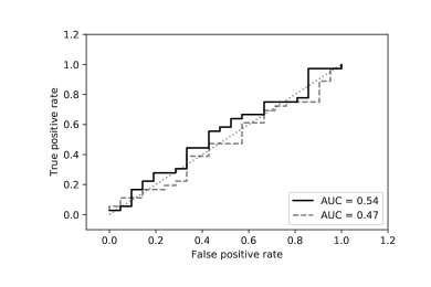
Block 3

Figure 13: ROC curves based on averaged probabilities for prediction blocks 1 and 3. Black model including the latent player abilities, grey-dashed baseline model, the dotted line is the line $y=x$.

Table 7: Area under the ROC curves based on averaged probabilities for each prediction block under both models.

Area under the curve values
	Block
Model	1	2	3	4	5
Baseline	0.47	0.60	0.53	0.55	0.61
Including latent player abilities	0.54	0.65	0.58	0.68	0.62

It is evident from both the figure and the table that including the latent player abilities in the model leads to a better predictive performance. We observe this increase across all blocks, although the difference between the models in block 5 is severely reduced compared to other blocks. The reasons for this reduction are twofold, the first being that given a near full season of data (2014/2015) on which we are predicting, the baseline model can reasonably accurately capture a team’s attack and defence parameters better than it can towards the start of the season. Secondly the last block of a season tends to be more volatile as some teams try out younger players (who are not observed in the data previously), and others have increased motivation to score more goals to try and win games, for example, to avoid relegation. Whence, we observe similar behaviour under both models, as we observe less players in a starting line-up, moving the model including player abilities towards the baseline model. However, overall, we can conclude that the inclusion of the latent player abilities in the model results in a better predictive performance throughout the 2014/2015 season.

The over/under betting market

As a final validation of the predictions made above, we consider both the baseline model and the model including the latent player abilities against the over/under betting market. We have odds data available to us (provided by Stratagem Technologies) for the 2014/2015 English Premier League season. Specifically, for each game we can bet on whether 2.5 goals will (over) or won’t (under) be scored. A betting strategy, similar to one based on the Kelly Criterion, is used to determine which games are bet on. We are unfortunately unable to disclose the full details of the betting strategy used as it is connected to the business decisions of Stratagem Technologies. Recall that we do not make predictions for promoted teams in prediction block 1, and hence we do not bet on these games. The cumulative return over the season for both models is shown in Figure 14. As above, it is clearly evident that including the latent player abilities in the model leads to a better performance over the baseline model. It is expected that the baseline model will (in general) lead to a zero or slightly negative return, which is what we observe here, with the model fluctuating around zero. If we placed $\pounds 100$ on each bet, our return under the model including the latent player abilities would be $\pounds 4486.73$ whilst under the baseline model it would be $-\pounds 378.54$. Another indication that including the latent player abilities is worthwhile. From the above sections we can conclude that the inclusion of the latent player abilities in the model results in better predictions over the 2014/2015 season.

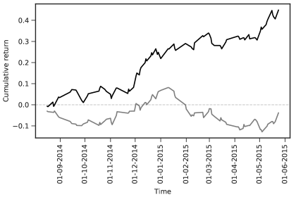
Figure 14: Cumulative return after betting on the over/under market for the 2014/2015 English Premier League season. Black model including the latent player abilities, grey baseline model.

5 Discussion

We have outlined a Bayesian model to establish player abilities. Our approach is computationally efficient and centres on variational inference methods. By adopting a Poisson model for occurrences of event types we are able to infer a player’s ability for a multitude of event types, distinguishing between any two given players (even if they always play for the same team). These inferences are reasonably accurate and have close ties to reality, as seen in Section 4.1. Furthermore, our approach allows the visualisation of differences between players for a specific ability through the marginal posterior variational densities. We believe the rankings of players shown in this paper could lead to debate, and offer some evidence to the hotly debated questions of football.

We also extended the Bayesian hierarchical model of Baio and Blangiardo, (2010) to include these latent player abilities. Through this model we captured a team’s propensity to score goals, including a team’s attacking ability, defensive ability and accounting for a home effect. We used output from this model to predict whether 2.5 goals would be scored in a game or not, observing an improvement in performance over the baseline model. A benefit of the prediction approach (and the block structure we implemented), is that it allowed us to see how our inferences about a player’s ability evolved through time, explicitly highlighting what impact fringe players can have when they start getting regular playing time, for example, Kane in Section 4.2.

Model assumptions and future work

In constructing our model a number of assumptions have been made. Here we discuss the more prominent of these with the hope they will be improved upon in future work. Firstly, the choice of the event types (and their construction from other event types). Event types were created with the help of expert football analysts and it is possible that using different analysts would lead to different event types. However we believe, with the analysts suggestions, we have managed to capture the composition of a football game reasonably well. In terms of approach, we believe this to be a good starting point and a sensible route as all combinations of events would be too large a space to consider. The exact combination of these event types is an open question and one for further research. An independence is also assumed between event types when they are grouped. The groupings of the events come from expert football analysts, so we have made the assumption that they truly reflect the final “grouped event,” for example, AntiPass. The interactions between all these events is incredibly nuanced and unknown. To our knowledge no one has explored this problem of how all events on a football pitch interact. It is this aspect that makes football hard to fully predict, given its variability. If you could define all the interactions, you would be able to fully predict a match. The question of how to fully define all interactions is an interesting one, and one that would likely lead to years of interesting research.

If a player is injured (or transfers to a different team during the year), they retain the same latent player abilities. We believe this to be a reasonable assumption but acknowledge some change in performance is likely if a player gets injured or moves team. We believe a change of performance would be quickly picked up by the model, as evidenced when we learn about new players, or players who start playing after being on the bench, see for example, Figure 11. An interesting extension may be to use a random walk on the variational parameters of a player when they change teams or return from injury.

When making predictions we use a predicted starting line-up from expert football analysts. This obviously will not be available to all, and a possible future option to be explored is to use a predicted starting line-up based on an average line-up from a predetermined number of past games. Also, we have not removed penalties as we are interested in goals scored by a player (by any means), an extension to the model may be to model penalty goals separately from other goals. We felt this would be an over complication to the model in this scenario, given its relative complexity already. It is interesting to note that the top 3 players for Goal did not score one penalty between them, so it is possible that the penalty goals do not affect the result too greatly.

Finally, we have included home effects for all event types. In the future, when considering a larger number of event types we may find that some home effects for certain events are negligible, and as such may not be required within the model, leading to situations where the model can be made more parsimonious. Whilst it has not been explored within this paper, an interesting application going forward would be to consider adding a player from one team into another, creating the effect of transferring in a player. Team performance could then be predicted incorporating the added player’s ability to see how a potential transfer target could affect results (or style of play). This of course could be done with multiple players, or entire fantasy squads, to help develop a better footballing strategy for the future.

In addition to addressing the above assumptions we plan three major ways of extending the current work. First, we intend to extend the variational approximation to allow for dependency among the latent abilities in the posterior. Allowing for correlations in $q(\cdot)$ will let the model infer higher posterior variances resulting in a more robust ranking of players, and possibly improved predictive power for tasks such as providing probabilities on the number of goals in a future match. From a modelling perspective, an extension is to let abilities change over time using a random walk across seasons and within seasons, which will be particularly useful when a substantial number of years of historical touch-by-touch data eventually becomes available. Finally, as the model gets applied to more competitions simultaneously it will be important to propose ways of scaling up the procedure. A topic worth investigating is how to best iteratively subsample the data for stochastic optimisation of the variational objective function. Of course, the approach proposed in this paper would also be applicable to other sports, and the authors believe such methods could easily be applied to basketball, hockey and rugby (with available data).

Appendix A Closed-form expression for the evidence lower bound

Recall that the log-likelihood to determine a player’s ability for a specific event ($\Delta_{i}^{e}$) is given by

$$\ell=\sum_{e\in E}\sum_{k=1}^{K}\sum_{j\in T_{k}}\sum_{i\in P_{k}^{j}}X_{i,k}^{e}\log{\left(\eta_{i,k}^{e}\tau_{i,k}\right)}-\eta_{i,k}^{e}\tau_{i,k}-\log{\left(X_{i,k}^{e}\,!\right)},$$ (19)

the evidence lower bound (ELBO) is

$$\textrm{ELBO}\left\{q\left(\Delta\right)\right\} =\sum_{e\in E}\sum_{k=1}^{K}\sum_{j\in T_{k}}\sum_{i\in P_{k}^{j}}\textrm{E}_{q\left(\Delta_{i}^{e}\right)}\left[\log\left\{\pi\left(\Delta_{i}^{e}\right)\right\}\right]+\textrm{E}_{q\left(\Delta_{i}^{e}\right)}\left[\log\left\{\pi\left(x|\Delta_{i}^{e},\phi_{i}^{e},\psi\right)\right\}\right]$$

$$\qquad\qquad\qquad\qquad\quad-\textrm{E}_{q\left(\Delta_{i}^{e}\right)}\left[\log\left\{q\left(\Delta_{i}^{e}|\phi_{i}^{e}\right)\right\}\right],$$ (20)

and

$$q\left(\Delta_{i}^{e}|\phi_{i}^{e}\right)\sim N\left(\mu_{\Delta_{i}^{e}},\sigma_{\Delta_{i}^{e}}^{2}\right).$$ (21)

Here the ELBO is available in closed-form. Below we consider the terms in (20) on an individual basis to derive this closed-form.

Let us begin by considering $\textrm{E}_{q\left(\Delta_{i}^{e}\right)}[\log\{q(\Delta_{i}^{e}|\phi_{i}^{e})\}]$. From (21) we have

$$\log\left\{q\left(\Delta_{i}^{e}\right)\right\}=-\frac{1}{2}\log\left(2\pi\sigma_{\Delta_{i}^{e}}^{2}\right)-\frac{\left(\Delta_{i}^{e}-\mu_{\Delta_{i}^{e}}\right)^{2}}{2\sigma_{\Delta_{i}^{e}}^{2}}.$$

Taking expectations gives

$$\textrm{E}_{q\left(\Delta_{i}^{e}\right)}\left[\log\left\{q\left(\Delta_{i}^{e}\Big{|}\phi_{i}^{e}\right)\right\}\right] =-\frac{1}{2}\log\left(2\pi\sigma_{\Delta_{i}^{e}}^{2}\right)$$

$$\qquad-\frac{1}{2\sigma_{\Delta_{i}^{e}}^{2}}\left[\textrm{E}\left\{\left(\Delta_{i}^{e}\right)^{2}\right\}-2\textrm{E}\left(\Delta_{i}^{e}\right)\mu_{\Delta_{i}^{e}}+\left(\mu_{\Delta_{i}^{e}}\right)^{2}\right]$$

$$=-\frac{1}{2}\log\left(2\pi\sigma_{\Delta_{i}^{e}}^{2}\right)$$

$$\qquad-\frac{1}{2\sigma_{\Delta_{i}^{e}}^{2}}\left\{\sigma_{\Delta_{i}^{e}}^{2}+\mu_{\Delta_{i}^{e}}^{2}-2\mu_{\Delta_{i}^{e}}^{2}+\mu_{\Delta_{i}^{e}}^{2}\right\}$$

$$=-\frac{1}{2}\log\left(2\pi\sigma_{\Delta_{i}^{e}}^{2}\right)-\frac{1}{2},$$ (22)

which is the negative entropy of the Gaussian distribution.

Let us now turn our attention to evaluating $\textrm{E}_{q\left(\Delta_{i}^{e}\right)}[\log\{\pi(\Delta_{i}^{e})\}]$, where $\Delta_{i}^{e}$ follows a $N(m,s^{2})$ prior. Therefore

$$\log\left\{\pi\left(\Delta_{i}^{e}\right)\right\}=-\frac{1}{2}\log\left(2\pi s^{2}\right)-\frac{\left(\Delta_{i}^{e}-m\right)^{2}}{2s^{2}}.$$

Hence

$$\textrm{E}_{q\left(\Delta_{i}^{e}\right)}\left[\log\left\{\pi\left(\Delta_{i}^{e}\right)\right\}\right] =-\frac{1}{2}\log\left(2\pi s^{2}\right)$$

$$\qquad-\frac{1}{2s^{2}}\left[\textrm{E}\left\{\left(\Delta_{i}^{e}\right)^{2}\right\}-2\textrm{E}\left(\Delta_{i}^{e}\right)m+m^{2}\right]$$

$$=-\frac{1}{2}\log\left(2\pi s^{2}\right)-\frac{\sigma_{\Delta_{i}^{e}}^{2}+\mu_{\Delta_{i}^{e}}^{2}-2m\mu_{\Delta_{i}^{e}}+m^{2}}{2s^{2}}.$$ (23)

Finally, let us consider $\textrm{E}_{q\left(\Delta_{i}^{e}\right)}[\log\{\pi(x|\Delta_{i}^{e},\phi_{i}^{e},\psi)\}]$. From (19) we have

$$\textrm{E}_{q\left(\Delta_{i}^{e}\right)}\left[\log\left\{\pi\left(x\Big{|}\Delta_{i}^{e},\phi_{i}^{e},\psi\right)\right\}\right]=\sum_{k=1}^{K}\underbrace{\textrm{E}\left\{X_{i,k}^{e}\log{\left(\eta_{i,k}^{e}\tau_{i,k}\right)}\right\}}_{\star}-\underbrace{\textrm{E}\left(\eta_{i,k}^{e}\tau_{i,k}\right)}_{\dagger}-\log{\left(X_{i,k}^{e}\,!\right)}.$$

Evaluating $\star$ first gives

$$\star =\textrm{E}\left[X_{i,k}^{e}\left\{\Delta_{i}^{e}+\tau_{i,k}\left(\lambda_{1}^{e}\sum_{i^{\prime}\in P_{k}^{j}}\Delta_{i^{\prime}}^{e}-\lambda_{2}^{e}\sum_{i^{\prime}\in P_{k}^{T_{k}\setminus j}}\Delta_{i^{\prime}}^{E\setminus e}\right)+\left(\delta_{T_{k}^{H},j}\right)\gamma^{\,e}+\log\left(\tau_{i,k}\right)\right\}\right]$$

$$=X_{i,k}^{e}\left\{\mu_{\Delta_{i}^{e}}+\tau_{i,k}\left(\lambda_{1}^{e}\sum_{i^{\prime}\in P_{k}^{j}}\mu_{\Delta_{i^{\prime}}^{e}}-\lambda_{2}^{e}\sum_{i^{\prime}\in P_{k}^{T_{k}\setminus j}}\mu_{\Delta_{i^{\prime}}^{E\setminus e}}\right)+\left(\delta_{T_{k}^{H},j}\right)\gamma^{\,e}+\log\left(\tau_{i,k}\right)\right\}.$$

Turning to $$\dagger$$, we have

$$\dagger =\textrm{E}\left[\exp\left\{\Delta_{i}^{e}+\tau_{i,k}\left(\lambda_{1}^{e}\sum_{i^{\prime}\in P_{k}^{j}}\Delta_{i^{\prime}}^{e}-\lambda_{2}^{e}\sum_{i^{\prime}\in P_{k}^{T_{k}\setminus j}}\Delta_{i^{\prime}}^{E\setminus e}\right)+\left(\delta_{T_{k}^{H},j}\right)\gamma^{\,e}\right\}\tau_{i,k}\right]$$

$$=\textrm{E}\left[\exp\left\{\left(1+\tau_{i,k}\lambda_{1}^{e}\right)\Delta_{i}^{e}\right\}\exp\left(\tau_{i,k}\lambda_{1}^{e}\sum_{i^{\prime}\in P_{k}^{j}\setminus i}\Delta_{i^{\prime}}^{e}\right)\exp\left(-\tau_{i,k}\lambda_{2}^{e}\sum_{i^{\prime}\in P_{k}^{T_{k}\setminus j}}\Delta_{i^{\prime}}^{E\setminus e}\right)\exp\left\{\left(\delta_{T_{k}^{H},j}\right)\gamma^{\,e}\right\}\tau_{i,k}\right]$$

$$=\exp\left\{\left(1+\tau_{i,k}\lambda_{1}^{e}\right)\mu_{\Delta_{i}^{e}}+\frac{\left(1+\tau_{i,k}\lambda_{1}^{e}\right)^{2}\sigma_{\Delta_{i}^{e}}^{2}}{2}\right\}\exp\left\{\tau_{i,k}\lambda_{1}^{e}\sum_{i^{\prime}\in P_{k}^{j}\setminus i}\mu_{\Delta_{i^{\prime}}^{e}}+\frac{\left(\tau_{i,k}\lambda_{1}^{e}\right)^{2}\displaystyle\sum_{i^{\prime}\in P_{k}^{j}\setminus i}\sigma_{\Delta_{i^{\prime}}^{e}}^{2}}{2}\right\}$$

$$\qquad\qquad\times\exp\left\{-\tau_{i,k}\lambda_{2}^{e}\sum_{i^{\prime}\in P_{k}^{T_{k}\setminus j}}\mu_{\Delta_{i^{\prime}}^{E\setminus e}}+\frac{\left(-\tau_{i,k}\lambda_{2}^{e}\right)^{2}\displaystyle\sum_{i^{\prime}\in P_{k}^{T_{k}\setminus j}}\sigma_{\Delta_{i^{\prime}}^{E\setminus e}}^{2}}{2}\right\}\exp\left\{\left(\delta_{T_{k}^{H},j}\right)\gamma^{\,e}\right\}\tau_{i,k}.$$

Therefore

$$\textrm{E}_{q\left(\Delta_{i}^{e}\right)}\left[\log\left\{\pi\left(x\Big{|}\Delta_{i}^{e},\phi_{i}^{e},\psi\right)\right\}\right] =\sum_{k=1}^{K}\left(X_{i,k}^{e}\left\{\mu_{\Delta_{i}^{e}}+\tau_{i,k}\left(\lambda_{1}^{e}\sum_{i^{\prime}\in P_{k}^{j}}\mu_{\Delta_{i^{\prime}}^{e}}-\lambda_{2}^{e}\sum_{i^{\prime}\in P_{k}^{T_{k}\setminus j}}\mu_{\Delta_{i^{\prime}}^{E\setminus e}}\right)\right.\right.$$

$$\qquad\qquad\qquad\left.+\left(\delta_{T_{k}^{H},j}\right)\gamma^{\,e}+\log\left(\tau_{i,k}\right)\right\}$$

$$\qquad-\left[\exp\left\{\left(1+\tau_{i,k}\lambda_{1}^{e}\right)\mu_{\Delta_{i}^{e}}+\frac{\left(1+\tau_{i,k}\lambda_{1}^{e}\right)^{2}\sigma_{\Delta_{i}^{e}}^{2}}{2}\right\}\right.$$

$$\left.\qquad\qquad\times\exp\left\{\tau_{i,k}\lambda_{1}^{e}\sum_{i^{\prime}\in P_{k}^{j}\setminus i}\mu_{\Delta_{i^{\prime}}^{e}}+\frac{\left(\tau_{i,k}\lambda_{1}^{e}\right)^{2}\displaystyle\sum_{i^{\prime}\in P_{k}^{j}\setminus i}\sigma_{\Delta_{i^{\prime}}^{e}}^{2}}{2}\right\}\right.$$

$$\left.\qquad\qquad\times\exp\left\{-\tau_{i,k}\lambda_{2}^{e}\sum_{i^{\prime}\in P_{k}^{T_{k}\setminus j}}\mu_{\Delta_{i^{\prime}}^{E\setminus e}}+\frac{\left(-\tau_{i,k}\lambda_{2}^{e}\right)^{2}\displaystyle\sum_{i^{\prime}\in P_{k}^{T_{k}\setminus j}}\sigma_{\Delta_{i^{\prime}}^{E\setminus e}}^{2}}{2}\right\}\right.$$

$$\left.\left.\qquad\qquad\qquad\times\exp\left\{\left(\delta_{T_{k}^{H},j}\right)\gamma^{\,e}\right\}\tau_{i,k}\right]-\log{\left\{X_{i,k}^{e}\,!\right\}}\right).$$ (24)

Thus, the closed form of the ELBO (20) is obtained through a combination of (22)–(24) whilst summing over $i$, $j$, $k$ and $e$, or explicitly

$$\textrm{ELBO}\left\{q\left(\Delta\right)\right\}=\sum_{e\in E}\sum_{j\in T_{k}}\sum_{i\in P_{k}^{j}}\textrm{\eqref{pexpect}}+\textrm{\eqref{pxexpect}}-\textrm{\eqref{qexpect}}.$$ (25)

Appendix B Top 10 results

In this section we detail top 10 rankings for a number of event types not presented in the Applications section—namely Shots, ShotStop, ChainEvents and AntiPass—which are presented in Tables 8, 9, 10 and 11 respectively. All 4 event types are of our own creation, made up of many other event types

• Shots: Goal, MissedShots, SavedShot, ShotOnPost.

• ShotStop: Challenge, Claim, Interception, KeeperPickup, Punch, Save, Smother, Tackle.

• AntiPass: BallRecovery, BlockedPass, Claim, Clearance, CornerAwarded, CrossNotClaimed, Interception, KeeperPickup, OffsideProvoked, Punch, Smother, Tackle.

Goal features in Shots, as a successful shot on target leads to a goal unless it becomes a SavedShot. ChainEvents is created by counting the number of instances a player is involved in the last 5 successful events leading to an event type contained within Shots, that is, the number of times a player is involved in a chain leading to a good attacking chance. The last 5 events were chosen as the length of the chain after discussion with expert football analysts, who thought that any further events back from the chance would have had little impact in creating it.

The top 10 for Shots consists entirely of strikers, the person seen as the main scorer of goals in a team, and thus, the person likely to have the most shots. The ranking appears sensible with the players heightened in our ranking (Aguero, Kane, Jovetic and A. Carroll) playing less time over the season due to injury, or mainly featuring as a substitute. The model suggests they took a large number of shots with the limited time they played. Suarez has an ability greater than any other player by a reasonable amount, which is expected given he had nearly 70 more shots than anyone else over the season. Over the 2013/2014 English Premier League season Suarez was regarded as the best player, winning many awards, it is therefore unsurprising that he features highly in many of the top 10 rankings.

The ranking for ShotStop is made up completely from goalkeepers, a natural conclusion given the event type. Lewis tops the ranking, although he only played 1 game and has a much larger standard deviation than anyone else. The goalkeepers for Fulham (Stockdale and Stekelenburg) played roughly half the season each, both stopping shots well (and at a similar level) when playing, for this reason they feature higher in our rankings than the observed order (determined by the total shots stopped over the season) suggests.

The top 10 for ChainEvents is similar in ways to that of GoalStop (presented in the main paper). It features a number of players with less playing time and therefore larger standard deviations. Whilst most of these players play a reasonable amount of time, from which to draw conclusions about their ability, the obvious outlier is Teixeira who played only 14 minutes (and has a very large standard deviation, comparatively). Again Suarez features highly in the rankings. The top 10 contains the creative players for each team, with that player for the top teams all featuring, Silva - Manchester City, Coutinho - Liverpool, Hazard - Chelsea. When we showed this ranking to expert football analysts there was a consensus that the ordering made sense (with the obvious exception of Teixeira).

The ranking for AntiPass consists of both defenders and defensive midfielders, both types of player whose job it is to disrupt play. Alcaraz and Kallstrom have comparatively larger standard deviations, but the remainder of the ranking appears sensible. The difference between successive rankings is small, and there is some suggestion that it is easier to distinguish between player attacking ability than player defensive ability (GoalStop, ShotStop, AntiPass). This would agree with some in the football community who view attacking as an individual ability, whereas defending is more of a team ability. Overall, all 4 of the rankings presented in this appendix appear largely sensible and agree with expert football analysts views.

Table 8: Top 10 shooters in the 2013/2014 English Premier League based on the 2.5% quantile of the marginal posterior variational density for each player, $q(\Delta_{i}^{\textrm{Shots}})$.

Shots - top 10
Rank	Player	Team	2.5%	Mean	Standard	Observed	Observed	Rank	Time
			quantile		deviation		rank	difference	played
1	Suarez	Liverpool	1.426	1.571	0.074	181	1	0	3185
2	Aguero	Manchester City	1.269	1.481	0.108	86	12	+10	1616
3	Dzeko	Manchester City	1.220	1.414	0.099	103	5	+2	2128
4	Kane	Tottenham Hotspur	1.038	1.413	0.191	28	126	+122	549
5	Bony	Swansea City	1.036	1.225	0.096	108	3	-2	2644
6	Sturridge	Liverpool	1.035	1.233	0.101	99	9	+3	2414
7	Jovetic	Manchester City	1.027	1.441	0.211	23	150	+143	440
8	Remy	Newcastle United	0.998	1.206	0.106	90	11	+3	2274
9	A. Carroll	West Ham United	0.982	1.258	0.141	51	53	+44	1200
10	Jelavic	Everton/Hull	0.978	1.210	0.118	72	18	+8	1804

Table 9: Top 10 shot-stoppers in the 2013/2014 English Premier League based on the 2.5% quantile of the marginal posterior variational density for each player, $q(\Delta_{i}^{\textrm{ShotStop}})$.

ShotStop - top 10
Rank	Player	Team	2.5%	Mean	Standard	Observed	Observed	Rank	Time
			quantile		deviation		rank	difference	played
1	Lewis	Cardiff City	2.413	2.823	0.209	23	369	+368	98
2	Mannone	Sunderland	2.394	2.485	0.046	453	8	+6	2767
3	Ruddy	Norwich City	2.312	2.394	0.042	555	1	-2	3679
4	Guzan	Aston Villa	2.258	2.343	0.043	512	2	-2	3684
5	Stockdale	Fulham	2.225	2.343	0.060	267	19	+14	1866
6	Marshall	Cardiff City	2.223	2.310	0.044	497	3	-3	3594
7	Stekelenburg	Fulham	2.218	2.340	0.062	252	24	+17	1790
8	Howard	Everton	2.218	2.306	0.045	483	5	-3	3575
9	Szczesny	Arsenal	2.199	2.286	0.045	484	4	-5	3594
10	Adrian	West Ham United	2.187	2.306	0.061	262	20	+10	1943

Table 10: Top 10 players involved in the last 5 interactions leading to a chance in the 2013/2014 English Premier League based on the 2.5% quantile of the marginal posterior variational density for each player, $q(\Delta_{i}^{\textrm{ChainEvents}})$.

ChainEvents - top 10
Rank	Player	Team	2.5%	Mean	Standard	Observed	Observed	Rank	Time
			quantile		deviation		rank	difference	played
1	Teixeira	Liverpool	2.419	3.291	0.444	5	474	+473	14
2	Suarez	Liverpool	2.408	2.486	0.040	546	1	-1	3185
3	Eikrem	Cardiff City	2.349	2.622	0.139	43	323	+320	229
4	Jovetic	Manchester City	2.303	2.525	0.113	72	250	+246	440
5	Silva	Manchester City	2.299	2.394	0.049	372	5	0	2308
6	Coutinho	Liverpool	2.241	2.338	0.049	362	6	0	2473
7	Taarabt	Fulham	2.230	2.426	0.100	89	214	+207	639
8	Ramirez	Southampton	2.218	2.415	0.101	92	208	+200	601
9	Aguero	Manchester City	2.213	2.330	0.060	251	32	+23	1616
10	Hazard	Chelsea	2.197	2.282	0.043	471	2	-8	3100

Table 11: Top 10 anti-passers in the 2013/2014 English Premier League based on the 2.5% quantile of the marginal posterior variational density for each player, $q(\Delta_{i}^{\textrm{AntiPass}})$.

AntiPass - top 10
Rank	Player	Team	2.5%	Mean	Standard	Observed	Observed	Rank	Time
			quantile		deviation		rank	difference	played
1	Alcaraz	Everton	2.864	3.031	0.085	135	292	+291	532
2	Vidic	Manchester United	2.855	2.940	0.043	520	35	+33	2256
3	Skrtel	Liverpool	2.814	2.885	0.036	759	2	-1	3468
4	Kallstrom	Arsenal	2.793	3.107	0.160	39	419	+415	144
5	Lovren	Southampton	2.789	2.865	0.039	640	10	+5	2993
6	Koscielny	Arsenal	2.783	2.860	0.039	632	11	+5	2980
7	Mulumbu	West Bromwich Albion	2.778	2.852	0.038	700	5	-2	3319
8	Azpilicueta	Chelsea	2.769	2.853	0.043	528	34	+26	2522
9	Jedinak	Crystal Palace	2.763	2.833	0.036	771	1	-8	3651
10	Fonte	Southampton	2.762	2.835	0.037	709	4	-6	3430

Appendix C ROC curves based on averaged probabilities

ROC curves based on the averaged probabilities discussed in Section 4.2 for each prediction block are presented in Figure 15.

Block 1

Block 2

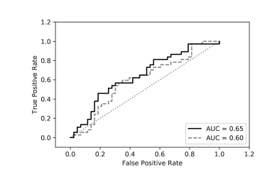
Block 3

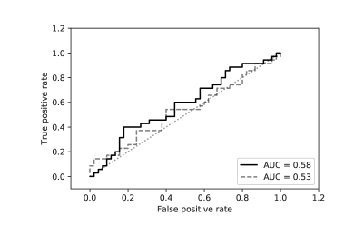
Block 4

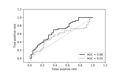
Block 5

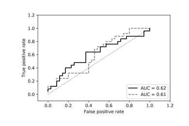
Figure 15: ROC curves based on averaged probabilities for each prediction block (see Section 4.2). Black model including the latent player abilities, grey-dashed baseline model, the dotted line is the line $y=x$.

References

-
AGR Analytics, (2016)
AGR Analytics (2016).
Explaining and examining per 90.
http://alexrathke.net/2016/07/explaining-and-examining-per-90. - Aitchison and Ho, (1989) Aitchison, J. and Ho, C. H. (1989). The multivariate Poisson-Log Normal distribution. Biometrika, 76(4):643–653.
- Anderson and Sally, (2013) Anderson, C. and Sally, D. (2013). The Numbers Game: Why Everything You Know About Football is Wrong. Penguin Books Limited.
- Baio and Blangiardo, (2010) Baio, G. and Blangiardo, M. (2010). Bayesian hierarchical model for the prediction of football results. Journal of Applied Statistics, 37(2):253–264.
-
BBC Business, (2016)
BBC Business (2016).
Premier League in record £5.14bn TV rights deal.
http://www.bbc.co.uk/news/business-31379128. -
Betfair, (2017)
Betfair (2017).
Over under 2.5 goals betting advice on Betfair.
https://betting.betfair.com/over-under-25-goals-betting-advice-on-betfair.html. -
betHQ, (2017)
betHQ (2017).
Over/under goals betting.
https://www.bethq.com/how-to-bet/articles/overunder-goals-betting. - Bialkowski et al., (2014) Bialkowski, A., Lucey, P., Carr, P., Yue, Y., Sridharan, S., and Matthews, I. (2014). Identifying team style in soccer using formations learned from spatiotemporal tracking data. In Data Mining Workshop (ICDMW), 2014 IEEE International Conference on, pages 9–14. IEEE.
- Bishop, (2006) Bishop, C. M. (2006). Pattern Recognition and Machine Learning. Information Science and Statistics. Springer.
- Blei and Jordan, (2006) Blei, D. M. and Jordan, M. I. (2006). Variational inference for Dirichlet process mixtures. Bayesian Analysis, 1(1):121–143.
- Blei et al., (2017) Blei, D. M., Kucukelbir, A., and McAuliffe, J. D. (2017). Variational inference: A review for statisticians. Journal of the American Statistical Association, 112(518):859–877.
- Bojinov and Bornn, (2016) Bojinov, I. and Bornn, L. (2016). The pressing game: Optimal defensive disruption in soccer. In MIT Sloan Sports Analytics Conference. MIT SSAC.
- Boshnakov et al., (2017) Boshnakov, G., Kharrat, T., and McHale, I. G. (2017). A bivariate Weibull count model for forecasting association football scores. International Journal of Forecasting, 33(2):458–466.
- Carbonetto and Stephens, (2012) Carbonetto, P. and Stephens, M. (2012). Scalable variational inference for Bayesian variable selection in regression, and its accuracy in genetic association studies. Bayesian Analysis, 7(1):73–108.
-
Cave and Miller, (2016)
Cave, A. and Miller, A. (2016).
Why football’s TV deal is a game changer.
http://www.telegraph.co.uk/investing/business-of-sport/premier-league-investors/. - Chib and Winkelmann, (2001) Chib, S. and Winkelmann, R. (2001). Markov chain Monte Carlo analysis of correlated count data. Journal of Business & Economic Statistics, 19(4):428–435.
- Curley and Roeder, (2016) Curley, J. P. and Roeder, O. (2016). English soccer’s mysterious worldwide popularity. https://contexts.org/articles/english-soccers-mysterious-worldwide-popularity/.
-
Deloitte, (2016)
Deloitte (2016).
Deloitte’s annual review of football finance.
https://www.deloitte.com/uk/en/pages/sports-business-group/articles/annual-review-of-football-finance.html. - Dixon and Coles, (1997) Dixon, M. J. and Coles, S. G. (1997). Modelling association football scores and inefficiencies in the football betting market. Journal of the Royal Statistical Society: Series C (Applied Statistics), 46(2):265–280.
- Dixon and Robinson, (1998) Dixon, M. J. and Robinson, M. (1998). A birth process model for association football matches. Journal of the Royal Statistical Society: Series D (The Statistician), 47(3):523–538.
- Du et al., (2009) Du, L., Ren, L., Carin, L., and Dunson, D. B. (2009). A Bayesian model for simultaneous image clustering, annotation and object segmentation. In Advances in Neural Information Processing Systems, pages 486–494.
- Franks et al., (2015) Franks, A., Miller, A., Bornn, L., and Goldsberry, K. (2015). Characterizing the spatial structure of defensive skill in professional basketball. The Annals of Applied Statistics, 9(1):94–121.
- Giordano et al., (2018) Giordano, R., Broderick, T., and Jordan, M. I. (2018). Covariances, robustness and variational bayes. The Journal of Machine Learning Research, 19(1):1981–2029.
- Groll et al., (2018) Groll, A., Kneib, T., Mayr, A., and Schauberger, G. (2018). On the dependency of soccer scores–a sparse bivariate Poisson model for the UEFA European football championship 2016. Journal of Quantitative Analysis in Sports, 14(2):65–79.
- Herbrich et al., (2007) Herbrich, R., Minka, T., and Graepel, T. (2007). Trueskill™: A Bayesian skill rating system. In Schölkopf, B., Platt, J. C., and Hoffman, T., editors, Advances in Neural Information Processing Systems 19, pages 569–576. MIT Press.
- Jordan et al., (1999) Jordan, M. I., Ghahramani, Z., Jaakkola, T. S., and Saul, L. K. (1999). An introduction to variational methods for graphical models. Machine Learning, 37(2):183–233.
- Joseph et al., (2006) Joseph, A., Fenton, N. E., and Neil, M. (2006). Predicting football results using Bayesian nets and other machine learning techniques. Knowledge-Based Systems, 19(7):544–553.
- Karlis and Ntzoufras, (2000) Karlis, D. and Ntzoufras, I. (2000). On modelling soccer data. Student, 3:229–245.
- Karlis and Ntzoufras, (2003) Karlis, D. and Ntzoufras, I. (2003). Analysis of sports data by using bivariate Poisson models. Journal of the Royal Statistical Society: Series D (The Statistician), 52(3):381–393.
- Karlis and Ntzoufras, (2009) Karlis, D. and Ntzoufras, I. (2009). Bayesian modelling of football outcomes: using the Skellam’s distribution for the goal difference. IMA Journal of Management Mathematics, 20(2):133–145.
- Kitani et al., (2011) Kitani, K. M., Okabe, T., Sato, Y., and Sugimoto, A. (2011). Fast unsupervised ego-action learning for first-person sports videos. In Computer Vision and Pattern Recognition (CVPR), IEEE Conference on, pages 3241–3248.
- Kucukelbir et al., (2017) Kucukelbir, A., Tran, D., Ranganath, R., Gelman, A., and Blei, D. M. (2017). Automatic differentiation variational inference. The Journal of Machine Learning Research, 18(1):430–474.
- Lee, (1997) Lee, A. J. (1997). Modeling scores in the Premier League: Is Manchester United really the best? Chance, 10(1):15–19.
- Lucey et al., (2013) Lucey, P., Oliver, D., Carr, P., Roth, J., and Matthews, I. (2013). Assessing team strategy using spatiotemporal data. In Proceedings of the 19th ACM SIGKDD International Conference on Knowledge Discovery and Data Mining, pages 1366–1374. ACM.
- Maclaurin et al., (2015) Maclaurin, D., Duvenaud, D., and Adams, R. P. (2015). Autograd: Effortless gradients in numpy. In ICML 2015 AutoML Workshop.
- Maher, (1982) Maher, M. J. (1982). Modelling association football scores. Statistica Neerlandica, 36(3):109–118.
- McHale et al., (2012) McHale, I. G., Scarf, P. A., and Folker, D. E. (2012). On the development of a soccer player performance rating system for the English Premier League. Interfaces, 42(4):339–351.
- McHale and Szczepański, (2014) McHale, I. G. and Szczepański, Ł. (2014). A mixed effects model for identifying goal scoring ability of footballers. Journal of the Royal Statistical Society: Series A (Statistics in Society), 177(2):397–417.
- Minka et al., (2018) Minka, T., Cleven, R., and Zaykov, Y. (2018). TrueSkill 2: An improved Bayesian skill rating system. Technical Report MSR-TR-2018-8, Microsoft.
- Raj et al., (2014) Raj, A., Stephens, M., and Pritchard, J. K. (2014). fastSTRUCTURE: Variational inference of population structure in large SNP data sets. Genetics, 197(2):573–589.
- Reep et al., (1971) Reep, C., Pollard, R., and Benjamin, B. (1971). Skill and chance in ball games. Journal of the Royal Statistical Society. Series A (General), pages 623–629.
- Ruiz and Perez-Cruz, (2015) Ruiz, F. J. R. and Perez-Cruz, F. (2015). A generative model for predicting outcomes in college basketball. Journal of Quantitative Analysis in Sports, 11(1):39–52.
-
Rumsby, (2016)
Rumsby, B. (2016).
Premier League clubs to share £8.3 billion TV windfall.
http://www.telegraph.co.uk/sport/football/12141415/Premier-League-clubs-to-share-8.3-billion-TV-windfall.html. - Saul and Jordan, (1996) Saul, L. and Jordan, M. I. (1996). Exploiting tractable substructures in intractable networks. In Advances in Neural Information Processing Systems 8, pages 486–492. MIT Press.
-
SPORTINGINDEX, (2017)
SPORTINGINDEX (2017).
Most popular spread betting markets.
https://www.sportingindex.com/#/o/learn/training-centre/most-popular-markets. - Stan Development Team, (2016) Stan Development Team (2016). PyStan: the Python interface to Stan, version 2.15.0.0.
- Sudderth and Jordan, (2009) Sudderth, E. B. and Jordan, M. I. (2009). Shared segmentation of natural scenes using dependent Pitman-Yor processes. In Advances in Neural Information Processing Systems, pages 1585–1592.
- Tunaru, (2002) Tunaru, R. (2002). Hierarchical Bayesian models for multiple count data. Austrian Journal of statistics, 31(3):221–229.
- Wainwright and Jordan, (2008) Wainwright, M. J. and Jordan, M. I. (2008). Graphical models, exponential families, and variational inference. Foundations and Trends in Machine Learning, 1(1-2):1–305.
- Whitaker et al., (2018) Whitaker, G. A., Silva, R., and Edwards, D. (2018). Visualizing a team’s goal chances in soccer from attacking events: A Bayesian inference approach. Big Data, 6(4):271–290.
- Yueh, (2014) Yueh, L. (2014). Exporting football. Why does the world love the English Premier League? http://www.bbc.co.uk/news/business-27369580.