Vision-based deep execution monitoring

Abstract

Execution monitor of high-level robot actions can be effectively improved by visual monitoring the state of the world in terms of preconditions and postconditions that hold before and after the execution of an action. Furthermore a policy for searching where to look at, either for verifying the relations that specify the pre and postconditions or to refocus in case of a failure, can tremendously improve the robot execution in an uncharted environment. It is now possible to strongly rely on visual perception in order to make the assumption that the environment is observable, by the amazing results of deep learning. In this work we present visual execution monitoring for a robot executing tasks in an uncharted Lab environment. The execution monitor interacts with the environment via a visual stream that uses two DCNN for recognizing the objects the robot has to deal with and manipulate, and a non-parametric Bayes estimation to discover the relations out of the DCNN features. To recover from lack of focus and failures due to missed objects we resort to visual search policies via deep reinforcement learning.

I Introduction

Robot perception has been amazingly boosted in recent years by deep learning results on object recognition [1, 2], relations recognition [3], visual question-answering (VQA)[4], activity recognition [5], image annotation [6], and navigation [7, 8] among other perceptual based abilities [9]. The upshot is that robots interaction with the real world nowadays seems to be in reach. The phenomenal success of deep learning across various disciplines motivates us to investigate whether useful representations in the robot task execution monitoring, in unknown environments, can be learned as well.

In this paper we address visual execution monitoring (VExM) in a dynamic uncharted lab environment, for high-level tasks. In order to monitor the state of execution we embed real time recognition of objects and relations which we call the visual stream, within a hybrid planning model. The visual stream is defined by a hierarchical model combining two deep convolution neural networks (DCNN)s [2] for object recognition, and a non-parametric Bayes model DPM[10] that uses the active features of the two DCNNs to segment the depth images collected during task execution. The combination of segmented depth and object labels allows to infer visual relations from the robot point of view. The hybrid planner, on the other hand, blends deterministic planning, with durable actions [11, 12, 13], with a contextually optimal visual search policy inferred from current state execution trained with DNN [14, 15], to cope with both task failures and loss of focus on the task. For policies inference the VExM builds states representations of the scene out of the visual stream results, which we call the mental maps, see Figure 1. Indeed, mental maps are used for both training the visual search policies and to recover focus on the current task, basing on deep reinforcement learning [14, 15]. An overview of a typical task execution in the proposed framework is given in Figure 1.

Though visual-based view of robot execution has been somehow faced previously by [16, 5, 17, 18, 7, 8], the proposed approach is completely novel in particular in terms of execution monitoring.

In this work perception is egocentric and we are considering high-level tasks, hence we are not considering motion control, 3D object pose estimation, nor navigation issues, we assume that all these problems are tackled by appropriate algorithms, see e.g. [19, 20, 21, 22, 23, 7].

In summary, we address visual execution monitoring as an hybrid deterministic/nondeterministic state machine streaming perceptual information, for both monitoring the execution and suitably directing visual perception. The VExM refocuses and redeems from a failure according to learned policies. Assuming that the visual stream provides a fully observable environment the VExM relies on learned policies [15] for focusing on the important objects involved in the task execution, and likewise to assess the discrepancy between the inferred state and the perceived one. Hence in case of failure the VExM can always resort to a recovery policy that ensures an optimized visual search to redeem into a state where execution can be retrieved.

II Related Work

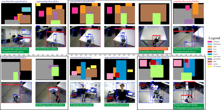
Figure 1: Visual execution monitoring (VExM) of the task take the Spraybottle and hand it to Person. Actions written in blue are provided by the planner, while those in red are generated by the visual search policy once a failure is detected. The post-conditions are shown below the images, those not verified, leading to a failure, are shown in red. The second and forth rows of images show the $bb$s of the objects and in red their relations discovered by the visual stream. The first and third rows of images represent the mental maps, here depth within the colored boxes is not visible. The hand misses the spraybottle (5th image), postcondition of action grasp $Holding(robot,spraybottle)$ fails while $Free(robot,robotHand)$ is verified. After a visual search the spraybottle is found on the floor. The involved relation in the parsed plan is updated from $On(spraybottle,table)$ to $On(spraybottle,floor)$ and the failed action is re-executed. A further visual search finds the subject, and finally the spray bottle is handed to her. Note the verification of the relations $CloseTo(robotHand,hand)$ and $Free(robot,robotHand)$, this last ensuring task goal success.

The earliest definitions of execution monitoring in nondeterministic environments have been introduced in [24, 25]. Since then an extraordinary amount of research has been done to address the nondeterministic response of the environment to robot actions. Several definitions of execution monitoring are reported in [26]. For high level robot tasks a review of these efforts is given in [27]. The role of perception in execution monitoring was already foreseen in the work of [28], likewise recovery from errors that could occur at execution time was already faced by [29]. Despite this foresight, the difficulties in dealing with scene recognition have directed the effort toward models managing the effects of actions such as [30, 31], allowing to execute actions in partially observable environments [32]. The integration of observations in high level monitor has been recently addressed by several authors, among which [33, 34]. Still, the breakthrough, is achieved with DCNN and in general with deep learning for perception [35], visual planning [18] and with deep Reinforcement Learning (RL) [14, 15].

Still for relations recognition, despite there is a great number of contributions [35, 3, 36] for 2D images, it is missed an appropriate method for robot execution. Hence we introduce a form of domain adaptation of the 2D images taken from ImageNet to segment the 3D images collected by the robot, basing on a DPM [10] that uses the active features of the recognized objects involved in the relation.

Another relevant aspect is visual search and the environment representation. Since the work of [14] a wealth of research has been done to make robust and extend RL [31, 30] to very large set of actions, in so developing a new amazing research area, deep RL [15, 37]. The only difficulty is the need to simulate the environment to perform the required huge collection of experiments. Hence a certain amount of research has been devoted to create new simulation environment such as [38, 8]. Here we contribute with a quite simple representation of the environment using the mental maps generated directly during robot experiments, basing on the depth segmentation and the bounding boxes of the recognized objects.

III Overview of our approach to visual execution monitoring

The robot execution monitor (VExM) we consider interacts both with the planning environment (described in Section V) and with the real world environment via the visual stream (Section IV). It exchanges information about the current state, the executed action and the action to be executed in such a state. This information concerns objects, terms and relations mentioned in the pre and postconditions of the action, and it is oriented by the visual search policies (Section V).

The planner environment has a deterministic component that infers the list of actions, pre and postconditions before execution starts, and a stochastic meta action which is the visual search. Since each of the plans forming a task has only one action affecting the world (see Section V) the beforehand inference of the specific plan goal is fine, because this is the only action that can fail, under our hypothesis of not considering robot control, which would lead to a continuous domain.

Example The task is illustrated in Figure 1. From a lexical component not described here, the task is parsed into a number of goals such as $holding(robot,sb)$, $closeTo(robotHand,hand)$. For each of these goals there is a plan issuing a sequence of actions, but for the visual search, which is a policy sequencing actions like look-Up, look-Down, turn-Left, turn-Right. Policies are learned basing on the actor critic paradigm [31, 30], exploiting the deep learning approach of [15].

At each state of the robot execution of the sequence of actions, the VExM verifies via the visual stream the feasibility of the next action visually assessing the relations mentioned in the action pre and postconditions specified in the state. The VExM uses this information to recompute transitions, according to a loss function that averages the discrepancy between the state (pre and postconditions of actions) inferred by the planner and the one observed by the visual stream (see Section VI).

If the objects of interest are out of the field of view some of the pre or postconditions will fail and the VExM appeals to the visual search to refocus on the object of interest. Typical examples are when the robot misses to position itself in front of a table or when it grasps something which falls down (see Figure 1). In these cases the visual search has to output the nice sequence of actions bringing the missed object back in the visual field.

In summary, with the VExM we do a step toward bridging the robot language and behavior between symbolic reasoning (via planning and logical inference) and deep learning with both the visual stream and the visual search paradigms. As a final remark the environment in principle it is not required to be completely static, still vision is egocentric and interaction with people is limited to few actions. An overview is given in Figure 1.

IV The visual stream

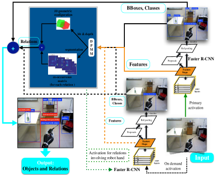
Figure 2: The models involved in the visual stream processing for the recognition of the current state $s_{t}$ concerning preconditions of action $a_{t}$ and postconditions of action $a_{t-1}$.

In this section we introduce the visual stream, which is the visual processing of the execution state. A schema is presented in Figure 2. Here a state $s_{t}$, $t$ in ${\mathbb{N}}$, specifies the precondition of action $a_{t}$, to be executed at state $s_{t}$, and the postconditions of action $a_{t-1}$, after its execution. For each state $s_{t}$ of the execution, the VExM opens an input-output channel with the visual stream, formed by a triple ${\mathcal{C}}_{t}=({\bf u},F,V)$, where ${\bf u}$ is a set of objects and relations on them, expected to hold at execution state $s_{t}$, $F$ is a buffer, of size $L$, of images from the video recorded by the robot and $V$ is the visual stream processing results, obtained with a hierarchy of deep models shown in Figure 2.

The models. There are essentially three models for the visual stream, which are called in parallel at execution time. The first model recognizes elements of the environment, a second model is trained to recognize those items that the robot can handle, and that can be occluded by the hand itself, a third model is trained to recognize the spatial relations, some of which are listed in Table I.

Step 1: recognizing objects in the scene. Let us consider the first two models concerning the objects. The first model is trained by collecting images of objects taken from both the robot environment, with an RGBD camera and with images of objects from ImageNet. The second model is trained with both images of human hands holding objects, and empty, and with the robot hand holding the objects of interest, and empty. Both these models are based on region proposal networks [2] and return in $V$ the objects label, their location in the image, and a probability for the images in $F$, given the $N$ objects in the model. Indeed, we are given, for each object in ${\bf u}$:

$$P(y=ob_{j}|{\bf x}_{\ell},\varphi_{\ell})=\arg\max_{{\bf x}_{\ell}\in F,\ell\in L}\sum_{\ell=1}^{N}h({\bf x}_{\ell},\varphi_{\ell})$$ (1)

Here $h({\bf x}_{\ell},\varphi_{\ell})$ is the softmax function of the region proposal network [2] applied to each image in $F$, with $\varphi_{\ell}$ the parameters.

Semi-supervised relations estimation. Despite recent contributions of several authors on 2d images, there are some difficulties to apply these approaches due to the relevance of depth to capture spatial relations, from the robot vantage point. To cope with these difficulties we have defined a model for relations adapting the active features of the trained DCNN [2], as described above, to the RGBD images collected by the robot. For each object $ob_{j}$ we estimate a statistics of the active features with dimension $38\times 50\times 512$, taken before the last pooling layer, say $Conv5$, at each pixel inside the recognized object bounding box $bb(ob_{j})$ (here we are referring to VGG, though we have considered also ZF, see [39, 40]).

Step 2: objects segmentation within the bounding boxes. Let the size of $bb(ob_{j})$ be $n=u\times v$ and let $z_{ji}=\sum_{k=1}^{d}x_{jik},i=1,..n$, where $x_{jik}$ is the normalized features value, with $d$ the feature dimension at pixel $i$, indexed w.r.t. the vectorized region of $bb(ob_{j})$. Let $Z=(z_{1},\ldots z_{n})^{\top}$ be sorted in descending order, and let $J$ be the corresponding pixel location of each value in $Z$ within the image resized according to $Conv5$. We consider the vector $\hat{Z}_{ob_{j}}$ formed by the first 25 elements of $Z$ (hence of $J$), which are the values exceeding the mean square of $Z$, turning out to be inside the object shape, in the RGBD-image resized according to the size of $Conv5$. Projecting the pixel locations $\hat{J}$ of these values on the resized image we obtain an observation matrix of size $25\times 4$, as we consider the RGB and depth channels. This data collection is repeated for about 100 images for each of the objects. With these features set, for each object we estimate a Dirichlet process mixture (DPM) [10]. Hence we have an infinite mixture model for each object, which amounts to have a set of parameters $\Theta_{h}=(\theta_{h,1},\ldots\theta_{h,k})$ for each object $ob_{h}$ with mixture components $k=1,..,q$, with $q$ inferred by the process (for more details about the DPM and its computation we refer the interested reader to [41], see also [42, 43]). Let $ob_{new}$ be an object in ${\bf u}$ - mentioned in the current open channel ${\mathcal{C}}_{t}$ - such that for some relation $R_{s}\in{\bf u}$, $ob_{new}$ belongs to the relation domain ${\mathcal{D}}_{R_{s}}$. Then we seek the model $\Theta_{h}\in\Theta$ and the component $\theta_{hk}\in\Theta_{h}$, which maximizes the probability of the active features selected as described above. Namely

$$\begin{array}[]{l}M(bb(ob_{new})|\Theta)=\\ \ \ \ \ \displaystyle{\arg\max_{\theta_{hk}\in\Theta}\{\sum_{h=1}^{N}\sum_{k=1}^{q}p_{hk}f(\hat{Z}|\theta_{h,k})\delta_{ob_{new}}({\mathcal{D}}_{\exists R_{s}})\}}\end{array}$$ (2)

Note that here $f(\cdot)$ is the normal distribution for which we assumed conjugate priors, $p_{hk}$ are the mixtures weights, $N$ is the number of objects, hence of $DPM$ models, and $\delta_{ob_{new}}({\mathcal{D}}_{\exists R_{s}})$ is 1 if $ob_{new}\in{\bf u}$ belongs to the domain of some $R_{s}\in{\bf u}$, and $0$ otherwise. The optimal parameters $\theta_{h,k})$ returns the component model that results in probability map within the bounding box of object $ob_{new}$, corresponding to the segmentation for $ob_{new}$, as shown in Figure 3 for the table and the screwdriver. Note that the segmentation is always relative to the region inside the bb. Note also that while the DPM model estimation can take several hours, its evaluation during execution, for the objects in ${\bf u}$, takes a little more than a second, being a second the time needed to run the networks, in order to obtain the active features for all the objects in ${\bf u}$.

Step 3: computing relations. Once the partial segmentations (according to the bbs) are available, we finally estimate the relations. For each relation $R_{s}$ we use basic geometric properties of the spatial configurations of the two bbs specifying it, together with reciprocal depth, basing on the eight volume-volume relation model of [44]. Here configurations with the same specification are considered to be topologically equivalent. Let $dmap=g(M(bb(ob_{i})|\Theta),M(bb(ob_{j})|\Theta^{\prime}),I_{D})$ be the projection of the mask of the probability map issued by the DPM on the depth map of the RGBD image in $F$. Let $p_{c}$ be the confidence in the specific $bb$s configuration according to the 9 volume-volume configurations for $dmap$, s.t $sump_{i}=1$. Without going into further details, we introduce a configuration probability for the $bb$s of the two objects $bb(ob_{i})$ and $bb(ob_{j})$ as $\nu_{ij}=\beta r^{-1}(A_{r}Dmap)p_{c}$ with $A_{r}$ the area of the two $bb$s, $r$ the number of relations and $\beta$ a further normalization constant.

Configurations of bounding boxes, even including depth, do not convey enough information, since they lack a semantic interpretation of the relations (for example in a specific image Inside and On can have the same configuration). Hence for each relation we define a co-occurrence matrix $N\times N$ amid all objects. The co-occurrence matrix reinforces the links between objects that have strong interactions and weakens those links that are already weak. We estimate the best decomposition $B=WH$ with $W\in{\mathbb{R}}_{+}^{N\times\Lambda}$ and $H\in{\mathbb{R}}_{+}^{\Lambda\times N}$, approaching the non-negative factorization (NMF) basing on the Bayesian NMF proposed in [45] to infer the best reducing factor $\Lambda$. Let $r$ be the number of relations, considering the tensor resulting from $N\times N\times r$, link values between $ob_{i}$ and $ob_{j}$ along the $r$ coordinate are given by $\lambda_{i,j,r}$. Given these findings, the probability that the relation $R_{s}$ holds for the observed objects $ob_{i},ob_{j}$ is given by the probability that the geometric configuration of $bb(ob_{I})$ and $bb(ob_{j})$ and their depth map (according to (2)) is correct, and by the likelihood of the relation semantics given by the co-occurrence matrix refining the relation domain. Let $\nu$ be the vector of the configuration values and let $\lambda_{ij}$ be the vector of link values for $ob_{i}$ and $ob_{j}$ and denote $z_{s}(i,j)$ the element wise normalized product of the two vectors. Then the probability of each relation is:

$$P(R_{s}|ob_{i},ob_{j})=z_{s}(i,j)p(ob_{i}|\varphi_{\ell})p(ob_{j}|\varphi_{\ell^{\prime}}),\ \ \ s=1,\ldots,r$$ (3)

We see that $z$ acts as a weight and it takes care of both the configuration of the bounding boxes according to the probability map given in (2) and of the domain of the relations, namely the statistics of their typical appearance in a scene. The chosen relation is the one maximizing the probability. Figure 3 show the result for the relation $On(screwdriver,table)$.

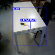
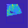
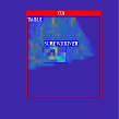
Figure 3: The segmentation map: segmentation of table and screwdriver from the $bb$s in the first image, according to (2), and relation found, according to (3).

V Hybrid planning environment

In this section we introduce the hybrid planning environment. This is made by a deterministic planner and a visual search policy. The visual search policy is required either to focus the robot toward the item of interest, so as to let the visual stream to deal with the preconditions of the action to be executed, or to recover from a failure. In our framework a failure occurs when the robot misses the objects of interest from the visual field, which is critical since in this case the execution state cannot be verified by the visual stream.

The deterministic planner The deterministic planner defines a nominal policy of high level actions to the goal. For the deterministic planner we consider a domain ${\mathcal{D}}$ formed by objects, relations and real numbers, which are represented in the robot language ${\mathcal{L}}$. A term of ${\mathcal{L}}$ can be an object $ob_{i}$ of the domain ${\mathcal{D}}$, a variable or a function $f:{\mathcal{D}}^{n}\mapsto{\mathcal{D}}$, such as actions. Relations (here assumed to be only binary), are defined exclusively for the specified set of objects of the domain, and are interpreted essentially as spatial relations such as On, CloseTo, Inside, Holding.

A robot task is defined by a list of plans $\langle{\mathcal{P}}_{1},\ldots,{\mathcal{P}}_{m}\rangle$; a plan ${\mathcal{P}}_{i}$ is defined as usual by an initial state and a set of rules (axioms) specifying the preconditions $H(a_{t})$ and postconditions $K(a_{t})$ of action $a(t)$, where $t$ is discrete time indexed in ${\mathbb{N}}$. To simplify we assume that preconditions and postconditions are conjunctions of ground atoms (binary relations), hence a state $s_{t}{=}H(a_{t})\cup K(a_{t})$. Though not necessary here, time maintains coherence between the deterministic part of the execution monitor and the Markov decision process underlying the visual search policy computation.

In our settings robot actions can be of two types: (1) supply actions, which are actions changing the state of the world, in so affecting some object in the world, such as grasp, hand-over, place, open, close; (2) egocentric actions, which are actions changing the state of the robot, such as move-Forward, approach $ob_{j}$ along a direction, or look-Up, look-down.

Egocentric actions, despite belong to the deterministic planner language, are mostly used within learned visual search policies, which are inferred according to the current state given a deep RL model [15]. On the other hand supply actions can have non-deterministic effects, which then lead to a failure, handled by a visual search recover policy.

According to these definitions a robot plan specifies at most one supply-action and this action is a durable action, defined by an action start and by an action end. Any other action in the plan is an egocentric action. In particular, given the initial state, each plan introduces at most a new primal object the robot can deal with and the relations of this object with the domain. An example is as follows: robot is holding an object, as a result of a previous plan, and it has to put it away on a toolbox. This ensures that recovery from a failure is circumscribed for each plan to a single supply action.

The task goal is unpacked into an ordered list of goals ${\mathcal{G}}{=}(G_{1},\ldots,G_{m})$ such that each $G_{i}$ is the goal of plan ${\mathcal{P}}_{i}$ in the list of plans forming a task. Given a goal $G_{i}$, if a plan ${\mathcal{P}}_{i}$ leading from the initial state to the goal exists, then a sequence of actions leading to the goal is inferred by the search engine [46]. Here plans are defined in PDDL [47].

We extend [46] parser to inferred plans, so as to obtain the initial state, the sequence of actions $(a_{0},\ldots,a_{n})$ leading to the goal, and the set of states $S_{{\mathcal{P}}_{i}}$ for each plan ${\mathcal{P}}_{i}$. This list forms the set of deterministic states and transitions.

In summary, the deterministic planner plays the role of an owner’s manual providing the robot with instructions about actions, properties, conditions that in principle should hold to accomplish the task.

The visual search Policy. Given the visual stream and the definition of a state we make here the assumption that the environment is fully observable. Hence we introduce a simple hybrid MDP, with discrete time, formed by the quintuple $(S,A,T,RW,\gamma)_{\mathcal{P}}$, for each plan ${\mathcal{P}}$. Here $S,A$ (set of states and actions for ${\mathcal{P}}$) are generated by the plan parser, $T:S\times A\times S\mapsto{\mathbb{R}}$ is the transition probability distribution, specifying the probability of moving between states, namely each $T_{ij}{=}\tau(s_{t+1}|s_{t},a_{t})$. $T$ has an added failure state. Initially $T$ (which is relative to a plan ${\mathcal{P}_{i}}$ hence should be written $T_{{\mathcal{P}}_{i}}$) is generated by the parser as a right stochastic $0{-}1$ matrix, and further updated by the VExM (see next section); $RW:S\mapsto{\mathbb{R}}$ is the expected reward and $\gamma\in[0,1]$ is the discount factor. In particular $T=\kappa(T_{pre}+T_{post})$, since states transitions are checked and updated by the VExM before and after action execution.

We recall here some notions from MDP and RL [31, 30]. The value $v$ of a state $s$ is the expected return starting from state $s_{t}$, namely $v(s){=}E[\sum_{k{=}0}\gamma^{k}RW_{t+k}|s_{t}{=}s]$, in matrix form (for each state) ${\bf v}{=}RW+\gamma T{\bf v}$. A policy $\pi:S\mapsto A$ specifies the probability of an action $a\in A$ given state $s\in S$, it is time-independent and has the Markov property. The action value function $Q_{\pi}(s,a)$ simply extends $v(s)$ to $v(s,a)$. The optimal action-value function $Q^{*}(s,a){=}\max_{\pi}Q_{\pi}(s,a)$ is the maximum action-value function over all policies and an optimal policy is one that achieves the optimal action-value function $\pi^{\star}(a,s){=}\arg\max_{a}Q^{\star}(a,s)$.

We are interested in an optimal visual search policy, which is a sequence of egocentric actions leading the robot to observe the scene so that the preconditions of the action to be executed or the postconditions of the executed action can be observed and verified. So the search policy drives the visual stream, which cannot be done by the blind deterministic planner. As noted above visual search can be composed of the following actions: look-Left, look-Right, look-Up, look-Down, move-Forward, move-Backward, turn-Left, turn-Right, with all these actions specified by precise quantities coherent with the underlying control, not mentioned here.

We approach the problem with a policy-based method by computing the parametrized policy $\pi(a|s,\psi)$ [48], where $\psi$ is the policy weight vector, hence $\pi(a|s,\psi){=}P(A_{t}{=}a|s_{t}{=}s,\psi_{t}{=}\psi)$, and the parameter update is:

$$\begin{array}[]{l}\psi_{t+1}{=}\psi_{t}+\\ \ \ \ \alpha\left(RW_{t+1}+\gamma\hat{v}(s_{t+1},{\bf w})-\hat{v}(s_{t},{\bf w})\right)\nabla_{\psi}\log\pi(a_{t}|s_{t},\psi)\end{array}$$ (4)

where $\hat{v}$ is a differentiable state value parametrization, ${\bf w}\in{\mathbb{R}}^{m}$ are state-value weights, $\psi$ the policy weights, and $\alpha>0$ step size parameter [30]. This is an actor-critic model in which the critic learns the action-value function while the actor learns the policy $\pi$. The goal is to learn a visual search policy. With A3C [15] have shown that a DNN can be used to approximate both the policy $\pi(a_{t}|s_{t},\psi)$ (softmax over actions) and the value function using two cost functions, the actor $L_{\pi}(\psi)$, which is derived from (4) with an extra entropy term to boost exploration in training, and the critic $L_{v}(\psi){=}(\sum_{i{=}0}\gamma^{i}RW_{t+i}-v(s_{t}|\psi)^{2}$. For optimization they used the standard non-centered RMSProp update: $g{=}\alpha g+(1-\alpha)\Delta\psi^{2}$, and $\psi\leftarrow\psi-\eta\Delta\psi(g+\epsilon)^{-1/2}$. Training has been done with A3C-LSTM [15], though with input the mental maps, described in the following. Our implementation follows https://github.com/miyosuda/async_deep_reinforce. A reward of 1 is issued whenever the primal object of the current plan appears in the mental map, then the robot restart the experiment.

Mental Maps There is an increasing interest in creating environment for deep RL, taking raw pixels as input, for example [38, 18, 8]. Here we use as input to the DNN the automatically generated mental maps, collected during experiments. The mental map takes as input an image from $F$ labeled by $V$ with stable bounding boxes $bb$s according to (1), the depth of the segmented objects within the bbs and a color code for each of the $N$ objects in the language and a link color, represented by a colored line, between the objects in a relation. It then forms a colored map which represents everything the robot knows about the world. In Figure 4 we show a short sequence of close mental maps generated for searching a person.

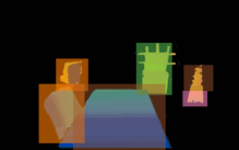
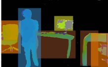
Figure 4: Mental Map generation for searching a person. The transparency shows the depth map of the labeled objects

VI Full execution algorithm

In this section we introduce the VExM algorithm. In the current implementation, given a task, the VExM is able to choose the list of goals on the basis of a naive Bayes classifier taking as input a bag of words, which we have not described here. Given the goals the choice of a deterministic plan for each goal is immediate. For each plan the VExM compute the parser, which in turns infers the ordered list of egocentric and supply actions $A$ and states $S$ to obtain the goal. We recall that a state $S_{t}$ specifies the set of preconditions and postconditions of action $a_{t}$, namely $H(a_{t})\cup K(a_{t})$. The algorithm starts with the ordered list of actions and states as computed by the parser for a plan ${\mathcal{P}}_{i}$ in the list of plans, and ends with the list of executed actions for ${\mathcal{P}}_{i}$, where only one action is a supply action. Note also that several events are here not taken into account, such as camera malfunctioning or other events concerning control and navigation that cannot be currently handled by the high-level VExM.

At each state $s_{t}$ the VExM computes via the visual stream the probability of each relation in ${\bf u}$, as described in Section IV and a loss. Then it updates the transition $T$, starting in $s_{t}$ with the truth values inferred by the deterministic planner. Because the monitor evaluates the loss for both preconditions and postconditions separately we indicate two loss functions, namely ${\mathcal{L}}(s_{t},X(a_{t}))$, with $X\in\{H,K\}$. Given $a_{t}$ at state $s_{t}$ and for $R_{s}\in{\bf u}_{t}$, $r$ the number of relations:

$$\begin{array}[]{ll}1.\ {\mathcal{L}}(s_{t},X(a_{t}))=\\ \ \ \ \ \displaystyle{\frac{1}{r}\sum_{R_{s}\in{\bf u}_{H(a_{t})}}\|1-P(R_{s}(ob_{i},ob_{j}))\|\delta_{ob_{i}}(R_{s})\delta_{ob_{j}}(R_{s})}\end{array}$$ (5)

Here $P(R_{s}(ob_{i},ob_{j}))$ is given in (3). According to (5) the transition matrix between states $s_{t}$ and $s_{t+1}$, is updated $T^{\prime}_{pre}=\left({\mathcal{L}}(s_{t},H(a_{t}))T_{pre}\right)/\left(2\sum_{s\in S}{\mathcal{L}}(s_{t},H(a_{t}))T_{pre}\right)$ and similarly for $T_{post}$, hence $T=\kappa(T_{pre}+T_{post})$. This include transition $\tau(s_{failure}|s_{t},a_{t})$ between state $s_{t}$ and the added failure state $s_{failure}$,(see Section V), so that the sum is always one. If the transition value to the failure state is greater than the transition value to the next state the visual search policy is called, independently of the planning requests. The algorithms are shown below.

Input: Ordered list $LI$ of actions and states for plan ${\mathcal{P}}_{i}$

Output: List $LE$ of experienced actions

while $LI\neq[]$ do

      Choose $a_{t}\in LI$, $t=0,\ldots,n$;

       Open $({\bf u},F,V)_{t}$ with visual stream;

       Compute $V_{H(a_{t})}$ and update transition $T_{pre}$ according to (5) for $H$;

      Compute Mmaps;

       if $a_{t}$ is visual search and args = $ob_{j}$ then  $[\widehat{{\bf u}}_{t},\widehat{F}_{t},\widehat{V}_{t},\pi(\dot{)},\savestack{\tmpbox}{\stretchto{\scaleto{\scalerel*[\widthof{Mmaps}]{\kern-0.6pt\bigwedge\kern-0.6pt}{\rule[-505.89pt]{4.30554pt}{505.89pt}}}{}}{0.5ex}}\stackon[1pt]{Mmaps}{\tmpbox}_{t}]$ = $Vsearch_{\pi}(a_{t},ob_{j},({\bf u},F,V)_{t},Mmaps)$;

       $\vec{a_{t}}\leftarrow\pi(s_{t}),{\bf u}\leftarrow\widehat{\bf u}_{t},F\leftarrow\widehat{F}_{t}$, $V_{t}\leftarrow\widehat{V}_{t},Mmaps=Mmaps\cup\{\savestack{\tmpbox}{\stretchto{\scaleto{\scalerel*[\widthof{Mmaps}]{\kern-0.6pt\bigwedge\kern-0.6pt}{\rule[-505.89pt]{4.30554pt}{505.89pt}}}{}}{0.5ex}}\stackon[1pt]{Mmaps}{\tmpbox}_{t}\}$;

       Execute $\vec{a_{t}}$ involving navigation and control, if required;

       Compute $V_{K(a_{t})}$ and update transition $T_{post}$ according to (5) for $K$;

      $LE=LE\cup\{\vec{a_{t}}\}$ ;

       else if $\tau(s_{failure}|s_{t},a_{t})<\tau(s_{t+1}|s_{t},a_{t})$ or $a_{t}$ is not supply-action then

             Execute action $a_{t}$ involving navigation and control, if required;

             Compute $V_{K(a_{t})}$ and update transition $T_{post}$ according to (5) for $K$;

             $LE=LE\cup\{\vec{a_{t}}\}$

       else if $\tau(s_{failure}|s_{t},a_{t})>\tau(s_{t+1}|s_{t},a_{t})$ and $a_{t}$ is supply-action then

             $[\widehat{{\bf u}}_{t},\widehat{F}_{t},\widehat{V}_{t},\pi(\dot{)},\savestack{\tmpbox}{\stretchto{\scaleto{\scalerel*[\widthof{Mmaps}]{\kern-0.6pt\bigwedge\kern-0.6pt}{\rule[-505.89pt]{4.30554pt}{505.89pt}}}{}}{0.5ex}}\stackon[1pt]{Mmaps}{\tmpbox}_{t}]$ = $Vsearch_{\pi}(a_{t},ob_{j},({\bf u},F,V)_{t},Mmaps)$;

             $\vec{a_{t}}\leftarrow\pi(s_{t}),{\bf u}\leftarrow\widehat{\bf u}_{t},F\leftarrow\widehat{F}_{t}$, $V_{t}\leftarrow\widehat{V}_{t},Mmaps=Mmaps\cup\{\savestack{\tmpbox}{\stretchto{\scaleto{\scalerel*[\widthof{Mmaps}]{\kern-0.6pt\bigwedge\kern-0.6pt}{\rule[-505.89pt]{4.30554pt}{505.89pt}}}{}}{0.5ex}}\stackon[1pt]{Mmaps}{\tmpbox}_{t}\}$;

            

            Execute $\vec{a_{t}}$ involving navigation and control, if required;

             Compute $V_{K(a_{t})}$ and update transition $T_{post}$ according to (5) for $K$;

            $LE=LE\cup\{\vec{a_{t}}\}$

       end if

      $T=\kappa(T_{pre}+T_{post})$;

       $t\leftarrow t+1$;

      

end while

if $Empty$ list of actions then

      return $LE$

else

      Failure

end if

Algorithm 1 Execution Monitor.

Input: $(a_{t},ob_{j},({\bf u},F,V)_{t},Mmaps)$

Output: $[\hat{{\bf u}}_{t},\hat{F}_{t},\hat{V}_{t},\pi_{t},\savestack{\tmpbox}{\stretchto{\scaleto{\scalerel*[\widthof{Mmaps}]{\kern-0.6pt\bigwedge\kern-0.6pt}{\rule[-505.89pt]{4.30554pt}{505.89pt}}}{}}{0.5ex}}\stackon[1pt]{Mmaps}{\tmpbox}_{t}]$

Compute $\pi(s_{t})$, for visual search $ob_{j}$, with $ob_{j}$ argument of $a_{t}$, input $Mmaps$, with A3C model;

Compute $\savestack{\tmpbox}{\stretchto{\scaleto{\scalerel*[\widthof{Mmaps}]{\kern-0.6pt\bigwedge\kern-0.6pt}{\rule[-505.89pt]{4.30554pt}{505.89pt}}}{}}{0.5ex}}\stackon[1pt]{Mmaps}{\tmpbox}$;

return $\widehat{{\bf u}}_{t},\widehat{F}_{t},\widehat{V}_{t}$, $\pi$

Algorithm 2 Visual Search $Vsearch$

VII Experiments and results

Platform Experiments for the VExM presented here have been done under different conditions in order to test different aspects of the model. To begin with, all experiments have been performed with a custom-made robot. A Pioneer 3 DX differential-drive robot is used as a compact mobile base. To interact with the environment we mounted a Kinova Jaco 2 arm with 6 degrees of freedom and a reach of 900mm and finally, for visual perception, we used an Asus Xtion PRO live RGB-D camera mounted on a Direct Perception PTU-46-17.5 pan-tilt unit.

Tasks We have considered two classes of tasks: (1) bring an object (spraybottle, screwdriver,hammer,cup) on the table or inside the shelf to a subject; (2) put-away object (screwdriver, hammer, spanner) in the toolbox. Each experiment in a class has been run 35 times manually driving the robot to collect images of the scene and 20 more times with the planning environment described in Section V, despite in a number of circumstances the grasping action has been manually helped, especially with small objects. From robot experiments we collected 120000 images, while from ImageNet we collected 25000 images. Table I shows the main relations, objects and actions considered in the tasks.

TABLE I: Subset of Objects, relations, supply-actions and egocentric actions of the robot language ${\mathcal{L}}$

Relations	Objects	Supply actions	Egocentric actions
CloseTo	Bottle	Close	Look-down
Found	Chair	Grasp	Look-left
Free	Cup	Open	Look-right
Holding	Floor	Hand-over	Look-up
Inside	Hammer	Place	Move-forward
On	Person	Lift	Move-backward
InFront	Spray Bottle	Push	Turn-left
Left	Screwdriver	Spin	Turn-right
Right	Shelf	Dispose	Localize
Under	Toolbox		Rise-arm
Behind	TV-Monitor		Lower-arm
Clear	Table		Close-Hand
Empty	Door		Open-Hand

Training We train the DCNN models using images taken from the ImageNet dataset, as well as images collected by the ASUS Xtion PRO RGB-D camera. We split the set of images in training and validation sets with a proportion of 80%-20%. We performed 70000 training iterations for each model on a PC equipped with 8 GPUs. Table II shows the object detection accuracy achieved by the two DCNN models dealing with the free and holding settings, respectively.

TABLE III: Relations detection accuracy

Relations	Accuracy
CloseTo	64%
Found	73%
Free	62%
Holding	79%
Inside	75%
On	83%
] InFront	78%
Left	68%
Right	72%
Under	71%
Behind	89%
Clear	67%
Empty	76%
Average	73.6%

Failures We examine the number of failures encountered during the executions of the tasks described above. A failure is recorded as soon as the state perceived by the visual stream via the DCNN and DPM models, does not match the post-conditions of the action executed. The histogram in Fig. 5 shows the probability that a failure is encounter while executing a particular action in relation to the object being involved. We note that, as expected, more complex actions like grasping and localizing show a higher probability of failure. Surprisingly, handing over an item shows a low failure probability, this is mainly attributed to the high adaptability of the subject involved in the action.

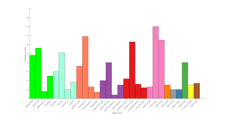
Figure 5: Histogram of action/objects failures

Recovery As explained in Section V, a visual search policy is employed as soon as a failure is detected in order to find the primary objects involved in the action that failed. Fig. 6 shows the success rate of the recovery via the use of a visual search policy for four different types of actions. Localization and manipulation actions show a higher recovery success rate, while recovering from a failed grasping seems to be the most problematic.

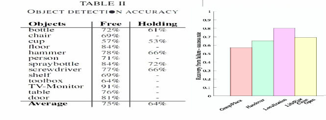
Figure 6: On the right the histogram of the recovery success ratios via visual search policy

References

- [1] A. Krizhevsky, I. Sutskever, and G. E. Hinton, “Imagenet classification with deep convolutional neural networks,” in NIPS 2012, 2012, pp. 1097–1105.
- [2] S. Ren, K. He, R. Girshick, and J. Sun, “Faster r-cnn: Towards real-time object detection with region proposal networks,” in NIPS, 2015, pp. 91–99.
- [3] C. Lu, R. Krishna, M. Bernstein, and L. Fei-Fei, “Visual relationship detection with language priors,” in ECCV, 2016, pp. 852–869.
- [4] S. Antol, A. Agrawal, J. Lu, M. Mitchell, D. Batra, Z. Lawrence, and D. Parikh, “Vqa: Visual question answering,” in (CVPR),2015, 2015, pp. 2425–2433.
- [5] M. Al-Omari, E. Chinellato, Y. Gatsoulis, D. C. Hogg, and A. G. Cohn, “Unsupervised grounding of textual descriptions of object features and actions in video.” in (KR),2016, 2016, pp. 505–508.
- [6] L. Feng and B. Bhanu, “Semantic concept co-occurrence patterns for image annotation and retrieval,” IEEE PAMI, vol. 38, no. 4, pp. 785–799, 2016.
- [7] P. Mirowski, R. Pascanu, F. Viola, H. Soyer, A. Ballard, A. Banino, M. Denil, R. Goroshin, L. Sifre, K. Kavukcuoglu, et al., “Learning to navigate in complex environments,” arXiv:1611.03673, 2016.
- [8] Y. Zhu, R. Mottaghi, E. Kolve, J. J. Lim, A. Gupta, L. Fei-Fei, and A. Farhadi, “Target-driven visual navigation in indoor scenes using deep reinforcement learning,” in (ICRA 2017). IEEE, 2017, pp. 3357–3364.
- [9] Y. LeCun, Y. Bengio, and G. Hinton, “Deep learning,” Nature, vol. 521, no. 7553, pp. 436–444, 2015.
- [10] T. S. Ferguson, “A bayesian analysis of some nonparametric problems,” Ann. Stat., pp. 209–230, 1973.
- [11] D. McDermott, M. Ghallab, A. Howe, C. Knoblock, A. Ram, M. Veloso, D. Weld, and D. Wilkins, “Pddl-the planning domain definition language,” 1998.
- [12] M. Helmert, “Concise finite-domain representations for pddl planning tasks,” Artif. Intel., vol. 173, no. 5-6, pp. 503–535, 2009.
- [13] M. Cashmore, M. Fox, D. Long, D. Magazzeni, B. Ridder, A. Carrera, N. Palomeras, N. Hurtós, and M. Carreras, “Rosplan: Planning in the robot operating system.” in ICAPS, 2015, pp. 333–341.
- [14] V. Mnih, K. Kavukcuoglu, D. Silver, A. A. Rusu, J. Veness, M. G. Bellemare, A. Graves, M. Riedmiller, A. K. Fidjeland, G. Ostrovski, et al., “Human-level control through deep reinforcement learning,” Nature, vol. 518, no. 7540, pp. 529–533, 2015.
- [15] V. Mnih, A. P. Badia, M. Mirza, A. Graves, T. Lillicrap, T. Harley, D. Silver, and K. Kavukcuoglu, “Asynchronous methods for deep reinforcement learning,” in ICML 2016, 2016, pp. 1928–1937.
- [16] I. Lenz, H. Lee, and A. Saxena, “Deep learning for detecting robotic grasps,” Int J. of Robotics Res., vol. 34, no. 4-5, pp. 705–724, 2015.
- [17] S. Vongbunyong, M. Pagnucco, and S. Kara, “Vision-based execution monitoring of state transition in disassembly automation.” IJAT, vol. 10, no. 5, pp. 708–716, 2016.
- [18] Y. Zhu, D. Gordon, E. Kolve, D. Fox, L. Fei-Fei, A. Gupta, R. Mottaghi, and A. Farhadi, “Visual semantic planning using deep successor representations,” CoRR, 2017.
- [19] P. Kaiser, D. Kanoulas, M. Grotz, L. Muratore, A. Rocchi, E. M. Hoffman, N. G. Tsagarakis, and T. Asfour, “An affordance-based pilot interface for high-level control of humanoid robots in supervised autonomy,” in (Humanoids 2016), 2016, pp. 621–628.
- [20] M. Rünz and L. Agapito, “Co-fusion: Real-time segmentation, tracking and fusion of multiple objects,” in (ICRA 2017), 2017, pp. 4471–4478.
- [21] M. Schwarz, H. Schulz, and S. Behnke, “Rgb-d object recognition and pose estimation based on pre-trained convolutional neural network features,” in (ICRA 2015), 2015, pp. 1329–1335.
- [22] C. Choi and H. I. Christensen, “Rgb-d object pose estimation in unstructured environments,” Robotics and Autonomous Systems, vol. 75, pp. 595–613, 2016.
- [23] A. Hornung, K. M. Wurm, M. Bennewitz, C. Stachniss, and W. Burgard, “Octomap: An efficient probabilistic 3d mapping framework based on octrees,” Autonomous Robots, vol. 34, no. 3, pp. 189–206, 2013.
- [24] R. E. Fikes, “Monitored execution of robot plans produced by strips,” SRI, Tech. Rep., 1971.
- [25] N. J. Nilsson, A hierarchical robot planning and execution system. SRI, 1973.
- [26] O. Pettersson, “Execution monitoring in robotics: A survey,” Robotics and Autonomous Systems, vol. 53, no. 2, pp. 73–88, 2005.
- [27] F. Ingrand and M. Ghallab, “Deliberation for autonomous robots: A survey,” Artificial Intelligence, vol. 247, pp. 10–44, 2017.
- [28] R. J. Doyle, D. J. Atkinson, and R. S. Doshi, “Generating perception requests and expectations to verify the execution of plans.”
- [29] D. E. Wilkins, “Recovering from execution errors in sipe,” Computational. Intelligence, vol. 1, no. 1, pp. 33–45, 1985.
- [30] R. S. Sutton and A. G. Barto, Reinforcement learning: An introduction (Second Edition), 1998,2017, vol. 1, no. 1.
- [31] D. P. Bertsekas and J. N. Tsitsiklis, “Neuro-dynamic programming: an overview,” in Decision and Control, 1995., vol. 1, 1995, pp. 560–564.
- [32] C. Boutilier, R. Reiter, M. Soutchanski, S. Thrun, et al., “Decision-theoretic, high-level agent programming in the situation calculus,” in AAAI/IAAI, 2000, pp. 355–362.
- [33] A. Hornung, S. Böttcher, J. Schlagenhauf, C. Dornhege, A. Hertle, and M. Bennewitz, “Mobile manipulation in cluttered environments with humanoids: Integrated perception, task planning, and action execution,” in (Humanoids 2014), 2014, pp. 773–778.
- [34] J. P. Mendoza, M. Veloso, and R. Simmons, “Plan execution monitoring through detection of unmet expectations about action outcomes,” in (ICRA 2015), 2015, pp. 3247–3252.
- [35] S. Guadarrama, L. Riano, D. Golland, D. Go, Y. Jia, D. Klein, P. Abbeel, T. Darrell, et al., “Grounding spatial relations for human-robot interaction,” in (IROS 2013), 2013, pp. 1640–1647.
- [36] A. Das, H. Agrawal, C. L. Zitnick, D. Parikh, and D. Batra, “Human attention in visual question answering: Do humans and deep networks look at the same regions?” arXiv preprint arXiv:1606.03556, 2016.
- [37] S. Levine, C. Finn, T. Darrell, and P. Abbeel, “End-to-end training of deep visuomotor policies,” Journal of Machine Learning Research, vol. 17, no. 39, pp. 1–40, 2016.
- [38] R. Mottaghi, H. Bagherinezhad, M. Rastegari, and A. Farhadi, “Newtonian scene understanding: Unfolding the dynamics of objects in static images,” in (CVPR 2016), 2016, pp. 3521–3529.
- [39] M. D. Zeiler and R. Fergus, “Visualizing and understanding convolutional networks,” in ECCV, 2014, pp. 818–833.
- [40] K. Simonyan and A. Zisserman, “Very deep convolutional networks for large-scale image recognition,” arXiv:1409.1556, 2014.
- [41] Y. W. Teh, “Dirichlet process,” in Encyclopedia of machine learning, 2011, pp. 280–287.
- [42] M. Sanzari, V. Ntouskos, and F. Pirri, “Bayesian image based 3d pose estimation,” in ECCV 2016, 2016, pp. 566–582.
- [43] F. Natola, V. Ntouskos, F. Pirri, and M. Sanzari, “Single image object modeling based on brdf and r-surfaces learning,” in CVPR 2016, 2016, pp. 4414–4423.
- [44] M. J. Egenhofer, “Topological relations in 3d,” Technical report, Tech. Rep., 1995.
- [45] V. Y. Tan and C. Févotte, “Automatic relevance determination in nonnegative matrix factorization with the/spl beta/-divergence,” IEEE PAMI, vol. 35, no. 7, pp. 1592–1605, 2013.
- [46] M. Helmert, “The fast downward planning system.” (JAIR), vol. 26, pp. 191–246, 2006.
- [47] S. Edelkamp and J. Hoffmann, “Pddl2. 2: The language for the classical part of the 4th international planning competition,” ICAPS 2004, 2004.
- [48] R. J. Williams, “Simple statistical gradient-following algorithms for connectionist reinforcement learning,” Machine learning, vol. 8, no. 3-4, pp. 229–256, 1992.