Optimisation of photometric stereo methods
by non-convex variational minimisation

Abstract

Estimating shape and appearance of a three dimensional object from a given set of images is a classic research topic that is still actively pursued. Among the various techniques available, photometric stereo is distinguished by the assumption that the underlying input images are taken from the same point of view but under different lighting conditions. The most common techniques provide the shape information in terms of surface normals. In this work, we instead propose to minimise a much more natural objective function, namely the reprojection error in terms of depth. Minimising the resulting non-trivial variational model for photometric stereo allows to recover the depth of the photographed scene directly. As a solving strategy, we follow an approach based on a recently published optimisation scheme for non-convex and non-smooth cost functions.

The main contributions of our paper are of theoretical nature. A technical novelty in our framework is the usage of matrix differential calculus. We supplement our approach by a detailed convergence analysis of the resulting optimisation algorithm and discuss possibilities to ease the computational complexity. At hand of an experimental evaluation we discuss important properties of the method. Overall, our strategy achieves more accurate results than competing approaches. The experiments also highlights some practical aspects of the underlying optimisation algorithm that may be of interest in a more general context.

1 Introduction

The reconstruction of three dimensional depth information given a set of two dimensional input images is a classic problem in computer vision. The class of methods fulfilling this task by inferring local shape from brightness analysis is called photometric methods BKP1986 ; Woehler2013 . They usually employ a static view point and variations in illumination to obtain the 3D structure. Fundamental photometric reconstruction processes are shape from shading (SFS) and photometric stereo (PS) BKP1986 . Shape from shading typically requires a single input image, whereas PS makes use of several input images taken from a fixed view point under different illumination. Photometric stereo incorporates SFS in the sense that SFS equations applied to each of the input images are integrated into a common PS process in order to obtain the 3D shape. This integrated model is usually formulated as an optimisation task that best explains the input images in terms of a pointwise estimation of shape and appearance.

The pioneer of the PS method was Woodham in 1978 Woodham1978a , see also Horn et al. HWS78 . The mathematical formulation of the PS problem is based on the use of the image irradiance equation (IIE) as in SFS for the individual input images, respectively. The image irradiance equation constitutes a relation between the image intensity and the reflectance map. The classic proceeding is thereby to consider Lambert’s law Lambert1760 for modelling the appearance of a shape given information on its geometry and albedo as well as the lighting in a scene. It has been shown that the orientation of a Lambertian surface can be uniquely determined from the resulting appearance variations provided that the surface is illuminated by at least three known, non-coplanar light sources, corresponding to at least three input images Woodham1980 . However, let us also mention the classic work of Kozera Kozera91 as well as Onn and Bruckstein OB90 where refined existence and uniqueness results are presented for the two-image case. As a beneficial aspect beyond the possible estimation of 3D shape, PS enables to compute an albedo map allowing to deal with non-uniform object materials or textured objects in a photographed scene.

As to complete our brief review of some general aspects of PS, let us note that it is possible to extend Woodham’s classic PS model as for instance to non-Lambertian reflectance as e.g. in Bartal2017 ; Ikehata2014a ; KhBoBr17 ; Mecca2016 ; TMDD2016 , or to take into account several types of lighting in a scene, see e.g. BJK07 ; QuDuWuCrLaDu17 . One may also consider a PS approach based on solving partial differential equations (PDEs) corresponding to ratios of the underlying IIE s, see for instance MeRoCr15 ; TMDD2016 . The latter approach makes it possible to compute the 3D shape directly whereas in most methods following the classic PS setting a field of surface normals is computed which needs to be integrated in another step; see e.g. BBQBD17 for a recent discussion of integration techniques.

Let us turn to the formulation of the PS approach we make use of. At this stage we keep the presentation rather general as we elaborate on the details that are of some importance in the context of applying our optimisation approach in Section 2. However, in order to explain the developments documented in this paper, it is useful to provide some formulae here.

Photometric 3D reconstruction is often formulated as an inverse problem: given an image $I$, the aim is to compute a depth map $z$ that best explains the observed grey levels of the data. To this end we use the IIE $I(u,v)=\mathcal{R}(z(u,v);\vec{s},\rho(u,v))$ where $\left(u,v\right)\in\Omega$ represent the coordinates over the reconstruction domain $\Omega\subseteq\mathbb{R}^{2}$ and where $\mathcal{R}$ denotes the reflectance map BKP1986 . This model describes interactions between the surface $z$ and the lighting $\vec{s}$. The vector $\rho$ represents reflectance parameters as e.g. the albedo, which can be either known or considered as hidden unknown parameters. For the sake of simplicity, we will consider in this paper only Lambertian reflectance without shadows, and we assume that the lighting of a photographed scene is directional and known. Moreover our camera is assumed to perform an orthographic projection. As in PS several input images $I^{i}$, $i\in\{1,\dots,m\}$ are considered under varying lighting $\vec{s}^{i}$, $i\in\{1,\dots,m\}$, the PS problem consists in finding a depth map $z$ that best explains all IIEs simultaneously:

$$I^{i}(u,v)=\mathcal{R}(z(u,v);\vec{s}^{i},\rho),\qquad i\in\{1,\ldots,m\}$$ (1)

Our contribution. Our aim is to obtain the solution $z$ of the PS problem, see also Figure 1 for an account. We show that estimating the optimal solution necessarily involves non-trivial optimisation methods, even with the simplest models for the reflectance function $\mathcal{R}$ and the most simple deviations from the model assumptions that may occur, i.e. we consider Lambertian reflectance without shadows and additive, zero-mean Gaussian noise.

To achieve our goal we propose a numerical framework to approximate an optimal solution which can be used to refine classic PS results. Our approach relies on matrix differential theory for analytic derivations and on recent developments in non-convex optimisation. In that novel framework for this class of problems we prove here the convergence of the optimisation method. The theoretical results are supplemented by a thorough numerical investigation that highlights some important observations on the optimisation routine.

The basic procedure of this work has been the subject of our conference paper HoQuBrRa16 , the results of which are mainly contained in the second, third and beginning of the fourth section of this article. Our current paper extends that previous work significantly by providing the mathematical validation of convergence and the extended analysis of the numerical optimisation algorithm. These are also exactly the core contributions of this paper. Moreover, we give a much more detailed description of the matrix calculus framework we employ.

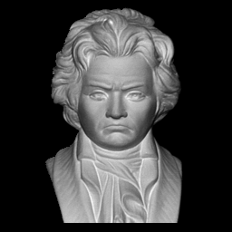
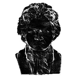
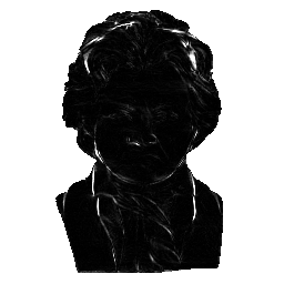
Example input image for PS	Classic PS with integration	Our method

Figure 1: From a set of $m\geq 3$ images (c.f. left), classic PS provides an albedo and a normal map which best explain the input images in the sense of a local, pointwise estimation. In a second step, the smooth depth map is estimated by integration. Yet, the final surface is not the best explanation of the images, as indicated by the reprojection error (c.f. energy in (5)) (middle). We display this using white for $2.5\cdot{}10^{-3}$ and black for zero. Instead of this local procedure, we propose to minimise the reprojection criterion in terms of the depth and the albedo, through global non-convex optimisation. Not only the images are better explained (right), but we also demonstrate that the 3D-reconstruction results are improved (c.f. Section 6).

2 Construction of our method and more related work

As shown by Woodham Woodham1980 , all surface normals can be estimated in the classic PS model without ambiguity, provided $m\geq 3$ input images and non-coplanar calibrated lighting vectors are given. In addition, the reflectance parameters (e.g. the albedo) can also be estimated. This is usually achieved by minimising the difference between the given data, i.e. the input images and the reprojection according to the estimated normal and albedo:

$$\operatorname*{arg\,min}_{\vec{n},\rho}\frac{1}{m}\iint_{\Omega}\sum_{i=1}^{m}\Phi\left(I^{i}-\mathcal{R}\left(\vec{n};\vec{s}^{i},\rho\right)\right)\mathop{\mathrm{\mathstrut d}}\nolimits\!{u}\mathop{\mathrm{\mathstrut d}}\nolimits\!{v}$$ (2)

with a penaliser $\Phi$. As a result, one obtains an approximation of the normal $\vec{n}(u,v)$ and the albedo $\rho(u,v)$ at each position $(u,v)$.

Since there is no coupling between the normals estimated in two neighboring pixels, those estimates are the optimal local explanations of the image, in the sense of the estimator $\Phi$. Yet, the estimated normal field is in general not integrable. Thus, the depth map that can be obtained by integration is not an optimal image explanation, but only a smooth explanation of the noisy normal field, c.f. Figure 1.

Instead of this pointwise joint estimation of the normal and the albedo, it is, as already mentioned in the introduction, possible to employ photometric ratios. Following that procedure means to divide the $i$-th by the $j$-th IIE in (1). This way, one obtains a homogeneous linear system in each normal vector that does not depend on the albedo, see MeRoCr15 . However, these ratios introduce additional difficulties in the models. It is common to assume that image data is corrupted by additive, zero-mean, Gaussian noise. In that case the maximum likelihood (ML) function should be chosen to be quadratic. Unfortunately, the ratio of two Gaussian random variables follows a Cauchy distribution Hinkley1969 . Thus, additional care has to be taken to find the most efficient penaliser. Another frequent assumption is that the estimated normal fields should be integrable, yet, this is a rather restrictive assumption. The normal field computed by many aforementioned PS approaches does not necessarily need to be integrable. Hence, the integration task is usually formulated as another optimisation problem which aims at minimising the discrepancy between the estimated normal field and that of the recovered surface. Following that approach we now go into some more details.

Assuming orthographic camera projection, the relation between the normal $\vec{n}(u,v)$ and the depth $z(u,v)$ is given by:

$$\vec{n}(u,v)\coloneqq\frac{1}{\sqrt{\|\nabla z(u,v)\|^{2}+1}}\left[-\nabla z(u,v),\,1\right]^{\top}$$ (3)

where $\nabla z$ is the gradient of $z$. Then, the best smooth surface explaining the computed normals can be estimated in several ways BBQBD17 , for instance by solving the variational problem:

$$\operatorname*{arg\,min}_{z}\iint_{\Omega}\Psi\left(\left\|\nabla z+\begin{bmatrix}\vec{n}_{1}/\vec{n}_{3}\\ \vec{n}_{2}/\vec{n}_{3}\end{bmatrix}\right\|^{2}\right)\mathop{\mathrm{\mathstrut d}}\nolimits\!{u}\mathop{\mathrm{\mathstrut d}}\nolimits\!{v}$$ (4)

where $\Psi$ is again some estimator function; see Durou2009 ; Harker2014 for some discussion.

One may realise that, at this stage of the process chain of PS with integration, the images are not explicitly considered anymore. Thus, the final surface is in general not necessarily optimal in the sense of the reprojection criterion. Regularising the normal field before integration Reddy2009 ; Zeisl2014 may also ensure integrability, but since such methods only use the normal field, and not the images, they may be unable to assert optimality with respect to the reprojection.

Global PS approaches solve the latter problem as they represent a way to ensure that the recovered surface is optimal with respect to the reprojection criterion. Moreover, it is possible to solve the system (1) directly in terms of the depth Clark1992 : this ensures both that the recovered surface is regular, and that it is optimal with respect to the reprojection criterion, calculated from the depth map $z$ and not from a non-integrable estimate of its gradient. Some PDE-based PS approaches have been recently proposed, and were shown to ease the resolution in particularly difficult situations such as pointwise lighting QuDuWuCrLaDu17 and specular reflectance TMDD2016 . To ensure robustness, such methods can be coupled with variational methods. In other words, the criterion which should be considered for ensuring optimality of a surface reconstruction by PS is not the local criterion (2), but rather:

$$\operatorname*{arg\,min}_{z,\rho}\frac{1}{m}\iint_{\Omega}\sum_{i=1}^{m}\Phi\left(I^{i}-\mathcal{R}\left(z;\vec{s}^{i},\rho\right)\right)\mathop{\mathrm{\mathstrut d}}\nolimits\!{u}\mathop{\mathrm{\mathstrut d}}\nolimits\!{v}$$ (5)

A theoretical analysis of the choice $\Phi(x)=|x|$, can be found in Chabrowski1993 . Numerical resolution methods based on proximal splittings were more recently introduced in SSVM2015a . Yet, this last work relies on an “optimise then discretise” approach which would involve non-trivial oblique boundary conditions (BC), replaced there for simplicity reasons by Dirichlet BC. Obviously, this represents a strong limitation which prevents working with many real-world data where this oblique BC is rarely available.

The optimisation problem (5) is usually non-linear and non-convex. The ratio procedure described earlier can be used: it simultaneously eliminates the albedo and the non-linear terms, c.f. Smith2016 ; Mecca2016 ; TMDD2016 ; GSSM2015 and obviously removes the bias due to non-integrability. But let us recall that it is only the best linear unbiased estimate, and also not the optimal one. To guarantee optimality, it is necessary to minimise the nonlinear, non-convex energy, i.e. without employing ratios. Other methods QuDuWuCrLaDu17 ; Queau2017 overcome the nonlinearity by absorbing it in the auxiliary albedo variable. Again, the solution is not that of the original problem (5) which remains, to the best of our knowledge, unsolved.

Solving (5) is a challenging problem. Efficient strategies to find the sought minimum are scarce. Recently Ochs et al. OCBP2013 proposed a novel method to handle such non-convex optimisation problems, called iPiano. A major asset of the approach is the extensive convergence theory provided in OCBP2013 ; P2016 . Because of this solid mathematical foundation we explore the iPiano approach in this work. The scheme makes explicit use of the derivative of the cost function, which in our case involves derivatives of matrix-valued functions, and we will employ as a technical novelty, matrix differential theory MN1985 ; MN2007 to derive the resulting scheme.

3 Non-convex discrete variational model for PS

In this section we describe the details of our framework for estimating both the depth and the (Lambertian) reflectance parameters over the domain $\Omega$.

3.1 Assumptions on the PS model

We assume $m\geq 3$ grey level images $I^{i}$, $i\in\{1,\dots,m\}$, are available, along with the $m$ lighting vectors $\vec{s}^{i}\in\mathbb{R}^{3}$, assumed to be known and non-coplanar. We also assume Lambertian reflectance and neglect shadows, which leads to the following well-known model:

$$\mathcal{R}\left(\vec{n}(u,v);\vec{s}^{i},\rho\right)\coloneqq\rho\left(u,v\right)\left\langle\vec{s}^{i}\,,\mathopen{}\vec{n}\left(u,v\right)\right\rangle$$ (6)

where $(u,v)\in\Omega$, $i=1,\ldots,m$ and $\rho(u,v)$ is the albedo at the surface point conjugated to position $(u,v)$, considered as a hidden unknown parameter. Let us note that real-world PS images can be processed by low-rank factorisation techniques in order to match the linear reflectance model (6), c.f. Wu2010 .

We further assume orthographic projection, hence the normal $\vec{n}(u,v)$ is given by (3). Then the reflectance model becomes a function of the depth map $z$:

$$\mathcal{R}\left(z;\vec{s}^{i},\rho\right)\coloneqq\frac{\rho\left(u,v\right)}{\sqrt{\|\nabla z(u,v)\|^{2}+1}}\left\langle\vec{s}^{i}\,,\mathopen{}\begin{bmatrix}-\nabla z(u,v)\\ 1\end{bmatrix}\right\rangle$$ (7)

with $(u,v)\in\Omega$, for all $i$. Eventually, we assume that the images $I^{i}$ differ from this reflectance model only up to additive, zero-mean, Gaussian noise. The ML estimator is thus the least-squares estimator $\Phi(x)=\frac{1}{2}x^{2}$, and the cost function in the reprojection criterion (5) becomes:

$$\mathcal{E}_{\mathcal{R}}\left(z,\rho;I\right)\coloneqq\frac{1}{2m}\iint_{\Omega}\sum_{i=1}^{m}\biggl{(}I^{i}-\mathcal{R}\left(z;\vec{s}^{i},\rho\right)\biggr{)}^{2}\mathop{\mathrm{\mathstrut d}}\nolimits\!{u}\mathop{\mathrm{\mathstrut d}}\nolimits\!{v}$$ (8)

3.2 Tikhonov regularisation of the model

Our energy in (8) only depends on the gradient $\nabla z$ and not on the depth $z(u,v)$ itself. As a consequence, solutions can only be determined up to an arbitrary constant. As a remedy we follow Mecca2016 and introduce a reference depth $z_{0}(u,v)$, thus regularising our initial model with a zero-th order Tikhonov regulariser controlled by a parameter $\lambda>0$:

$$\operatorname*{arg\,min}_{z,\rho}\mathcal{E}_{\mathcal{R}}\left(z,\rho;I\right)+\frac{\lambda}{2}\iint_{\Omega}\left(z-z_{0}\right)^{2}\mathop{\mathrm{\mathstrut d}}\nolimits\!{u}\mathop{\mathrm{\mathstrut d}}\nolimits\!{v}$$ (9)

In practice, $\lambda$ can be set to any small value, so that a solution of (9) lies as close as possible to a minimiser of (8). In all our experiments we set $\lambda:=10^{-6}$ and $z_{0}$ as the classic PS solution followed by least-squares integration BBQBD17 .

3.3 Discretisation

As already mentioned, “optimise then discretise” approaches for solving (9), such as SSVM2015a , involve non-trivial BC. Hence, we prefer a “discretise then optimise”, finite dimensional formulation of the variational PS problem (9).

In our discrete setting we are given $m$ images $\vec{I}^{i}$, $i\in\{1,\dots,m\}$, with $n$ pixels labelled with a single index $j$ running from 1 to $n$. We discretise (9) in the following way:

$$\operatorname*{arg\,min}_{\vec{z},\rho\in\mathbb{R}^{n}}\biggl{\{}\frac{1}{2m}\sum_{j}\biggl{\|}\vec{I}_{j}-\frac{\rho_{j}}{\sqrt{\left\lVert\nabla\vec{z}_{j}\right\rVert^{2}+1}}\vec{S}\begin{bmatrix}-\nabla\vec{z}_{j}\\ 1\end{bmatrix}\biggr{\|}^{2}\\ +\frac{\lambda}{2}\left\lVert\vec{z}_{j}-{\vec{z}_{0}}_{j}\right\rVert^{2}\biggr{\}}$$ (10)

where $\vec{I}_{j}\coloneqq[\vec{I}^{1}_{j},\dots,\vec{I}^{m}_{j}]^{\top}\in\mathbb{R}^{m}$ is the vector of intensities at pixel $j$, $\nabla\vec{z}_{j}$ represents now a finite difference approximation of the gradient of $\vec{z}$ at pixel $j$, and $\vec{S}=[\vec{s}^{1},\ldots,\vec{s}^{m}]^{\top}\in\mathbb{R}^{m,3}$ is a matrix containing the stacked $m$ lighting vectors $\vec{s}^{i}$.

We remark that the matrix $\vec{S}$ can be decomposed into two sub-matrices $\vec{S}_{\ell}$ and $\vec{S}_{r}$ of dimensions $m\times 2$ and $m\times 1$ such that $\vec{S}\coloneqq\begin{bmatrix}\vec{S}_{\ell}&\vec{S}_{r}\end{bmatrix}$, and so that

$$\vec{S}\begin{bmatrix}-\nabla\vec{z}_{j}\\ 1\end{bmatrix}=-\vec{S}_{\ell}\nabla\vec{z}_{j}+\vec{S}_{r}$$ (11)

Let us also introduce a $2n\times n$ block matrix $\vec{M}$, such that each block $\vec{M}_{j}$ is a $2\times n$ matrix containing the finite difference coefficients used for approximating the gradient:

$$\vec{M}\coloneqq\begin{bmatrix}\vec{M}_{1}\;\ldots\;\vec{M}_{n}\end{bmatrix}^{\top}\in\mathbb{R}^{2n,n},\qquad\vec{M}_{j}\vec{z}=\nabla\vec{z}_{j}\in\mathbb{R}^{2}$$ (12)

We further introduce the aliases

$$\vec{A}_{j}(\vec{z},\rho)\coloneqq-\frac{\rho_{j}}{\sqrt{1+\left\lVert\vec{M}_{j}\vec{z}\right\rVert^{2}}}\vec{S}_{\ell}\in\mathbb{R}^{m,2}$$ (13)

and

$$\vec{b}_{j}(\vec{z},\rho)\coloneqq\vec{I}_{j}-\frac{\rho_{j}}{\sqrt{1+\left\lVert\vec{M}_{j}\vec{z}\right\rVert^{2}}}\vec{S}_{r}\in\mathbb{R}^{m}$$ (14)

and stack them, respectively, in a block-diagonal matrix

$$\vec{A}(\vec{z},\rho)\coloneqq\begin{bmatrix}\vec{A}_{1}(\vec{z},\rho)&\leavevmode\nobreak\ &\leavevmode\nobreak\ \\ \leavevmode\nobreak\ &\ddots&\leavevmode\nobreak\ \\ \leavevmode\nobreak\ &\leavevmode\nobreak\ &\vec{A}_{n}(\vec{z},\rho)\end{bmatrix}\in\mathbb{R}^{mn,2n}$$ (15)

and a vector

$$\vec{b}(\vec{z},\rho)\coloneqq\begin{bmatrix}\vec{b}_{1}(\vec{z},\rho)\\ \vdots\\ \vec{b}_{n}(\vec{z},\rho)\end{bmatrix}\in\mathbb{R}^{mn}$$ (16)

Using these notational conventions as well as

$$f(\vec{z},\rho)\coloneqq\frac{1}{2m}\left\lVert\vec{A}(\vec{z},\rho)\vec{M}\vec{z}-\vec{b}(\vec{z},\rho)\right\rVert_{2}^{2}$$ (17)

and

$$g(\vec{z})\coloneqq\frac{\lambda}{2}\left\lVert\vec{z}-\vec{z}_{0}\right\rVert_{2}^{2}$$ (18)

the task in (10) can be rewritten compactly as

$$\operatorname*{arg\,min}_{\vec{z},\rho\in\mathbb{R}^{n}}\left\{f(\vec{z},\rho)+g(\vec{z})\right\}$$ (19)

which is the discrete PS model we propose to tackle in this paper. Observe that, if $\vec{A}(\vec{z},\rho)$ and $\vec{b}(\vec{z},\rho)$ were constant, problem (19) would be a linear least squares problem with respect to $\vec{z}$.

Let us remark that (19) can be easily extended to include more realistic reflectance Ju2013 ; KhBoBr17 and lighting BMVC.28.128 ; QuDuWuCrLaDu17 models, as well as more robust estimators Ikehata2014a ; Queau2017 : this only requires to change the definition of $f$, which stands for the global reprojection error $\mathcal{E}_{\mathcal{R}}$.

3.4 Alternating optimisation strategy

In order to ensure applicability of our method to real-world data, the albedo $\rho$ cannot be assumed to be known. Inspired by the well-known Expectation-Maximisation algorithm, we treat $\rho$ as a hidden parameter, and opt for an alternating strategy which iteratively refines the depth with fixed albedo, and the hidden parameter with fixed depth:

$$\vec{z}^{(k+1)} =\operatorname*{arg\,min}_{\vec{z}}\left\{f\left(\vec{z},\rho^{(k)}\right)+g(\vec{z})\right\}$$ (20)

$$\rho^{(k+1)} =\operatorname*{arg\,min}_{\rho}\left\{f\left(\vec{z}^{(k+1)},\rho\right)+g\left(\vec{z}^{(k+1)}\right)\right\}$$ (21)

starting from $\vec{z}^{(0)}=\vec{z}_{0}$ and taking as $\rho^{(0)}$ the albedo obtained by the classic PS approach Woodham1980 . Of course, the choice of a particular prior $\vec{z}_{0}$ has a direct influence on the convergence of the algorithm. The proposed scheme globally converges towards the solution, even with a trivial prior $\vec{z}_{0}\equiv\text{constant}$, but convergence is very slow in this case. Thus the proposed method should be considered as a post-processing technique to refine classic PS approaches, rather than as a standalone PS method.

Now, let us comment on the two optimisation problems in (20). Updating $\rho$ amounts pointwise to a linear least-squares problem, which admits the following closed-form solution at each pixel:

$$\rho^{(k+1)}_{j}=\frac{\sqrt{1+\|\vec{M}_{j}\vec{z}^{(k+1)}\|^{2}}\sum\limits_{i=1}^{m}\vec{I}^{i}_{j}{\vec{s}^{i}}^{\top}\begin{bmatrix}-\vec{M}_{j}\vec{z}^{(k+1)}\\ 1\end{bmatrix}}{\sum\limits_{i=1}^{m}\left({\vec{s}^{i}}^{\top}\begin{bmatrix}-\vec{M}_{j}\vec{z}^{(k+1)}\\ 1\end{bmatrix}\right)^{2}}$$ (22)

The computation of $\vec{z}^{(k+1)}$ is considerably harder, and it is dealt with in the following paragraphs.

4 An inertial proximal point algorithm for PS

In this section we discuss the numerical solution strategy of our problem (20). We especially discuss the main difficulty within this strategy, that is to compute the gradient with respect to $\vec{z}$ for the function $f$ in (17). Apart from the explicit formula for this gradient we also investigate an approximation leading to efficient computations on a desktop computer with an intel CPU.

4.1 The iPiano algorithm

We will now make precise the iPiano algorithm OCBP2013 for our problem (20). Since the albedo is fixed for the purpose of the corresponding optimisation stage, we denote $f(\vec{z})=f(\vec{z},\rho^{(k)})$. The iPiano algorithm seeks a minimiser of

$$\min_{\vec{x}\in\mathbb{R}^{n}}\left\{f(\vec{x})+g(\vec{x})\right\}$$ (23)

where $g\colon\mathbb{R}^{n}\to\mathbb{R}$ is convex and $f\colon\mathbb{R}^{n}\to\mathbb{R}$ is smooth. What makes iPiano appealing is the fact that $g$ must not necessarily be smooth and $f$ is not required to be convex. This allows manifold designs of novel fixed-point schemes. In its general form it evaluates

$$\operatorname{prox}_{\alpha g}\left(\vec{z}^{(k)}-\alpha\nabla f(\vec{z}^{(k)})+\beta(\vec{z}^{(k)}-\vec{z}^{(k-1)})\right)$$ (24)

where the proximal operator is given by

$$\operatorname{prox}_{\alpha g}\left(\vec{z}\right)\coloneqq\operatorname*{arg\,min}_{\vec{x}}\left\{\frac{1}{2}\left\lVert\vec{x}-\vec{z}\right\rVert^{2}+\alpha g\left(\vec{x}\right)\right\}$$ (25)

and which goes back to Moreau M1965 . Before we can define the final algorithm we also need to determine the gradient of $f$.

4.2 Matrix Calculus

We will first recall some general rules to derive the Jacobian of a matrix valued function, before we apply these rules to our setting in the next section.

In our setting the main difficulty is that the matrix $\vec{A}$ depends on our sought unknown $\vec{z}$. In order to state a useful representation of arising differential expressions we have to resort to matrix differential calculus. We refer to MN1985 ; P1985 ; MN2007 ; PP2008 for a more in-depth representation. A key notion is the definition of the Jacobian of a matrix, which can be obtained in several ways. In this paper we follow the one given in MN1985 .

Definition 1 (Jacobian of a Matrix Valued Function)

Let $\vec{A}$ be a differentiable $m\times p$ real matrix function of an $n\times q$ matrix $\vec{X}$ of real variables, i.e. $\vec{A}=\vec{A}(\vec{X})$. The Jacobian matrix of $\vec{A}$ at $\vec{X}$ is the $mp\times nq$ matrix

$$D\left[\vec{A}\right]\left(\vec{X}\right)\coloneqq\frac{\mathop{\mathrm{\mathstrut d}}\nolimits\!\operatorname{vec}{\left(\vec{A}\left(\vec{X}\right)\right)}}{\mathop{\mathrm{\mathstrut d}}\nolimits(\operatorname{vec}{\vec{X}})^{\top}}$$ (26)

where $\operatorname{vec}{(\cdot)}$ corresponds to the vectorisation operator described in HJ1994 (Definition 4.29). This operator stacks column-wise all the entries from its matrix argument to form a large vector.

Here, differentiability of a matrix valued function means that the corresponding vectorised function is differentiable in the usual sense. By this definition the computation of a matrix Jacobian can be reduced to computing a Jacobian for a vector valued function.

Example 1

Let $\vec{A}(\vec{x})\in\mathbb{R}^{m,m}$ be a differentiable diagonal matrix

$$\vec{A}(\vec{x})=\begin{bmatrix}a_{1}(\vec{x})&&\\ &\ddots&\\ &&a_{m}(\vec{x})\end{bmatrix}\qquad\text{for all }\vec{x}\in\mathbb{R}^{n}$$ (27)

then the Jacobian matrix of $\vec{A}$ at $\vec{x}$ has the form

$$D\left[\vec{A}(\vec{x})\right](\vec{x})=\frac{\mathop{\mathrm{\mathstrut d}}\nolimits\!missing}{\mathop{\mathrm{\mathstrut d}}\nolimits\!\vec{x}^{\top}}\begin{bmatrix}a_{1}(\vec{x})\\ \vec{0}_{m,1}\\ a_{2}(\vec{x})\\ \vec{0}_{m,1}\\ \vdots\\ a_{m}(\vec{x})\end{bmatrix}=\begin{bmatrix}\frac{\partial a_{1}(\vec{x})}{\partial\vec{x}_{1}}&\cdots&\frac{\partial a_{1}(\vec{x})}{\partial\vec{x}_{n}}\\ &\vec{0}_{m,n}&\\ \frac{\partial a_{2}(\vec{x})}{\partial\vec{x}_{1}}&\cdots&\frac{\partial a_{2}(\vec{x})}{\partial\vec{x}_{n}}\\ &\vec{0}_{m,n}&\\ &\vdots&\\ \frac{\partial a_{m}(\vec{x})}{\partial\vec{x}_{1}}&\cdots&\frac{\partial a_{m}(\vec{x})}{\partial\vec{x}_{n}}\end{bmatrix}$$ (28)

where $\vec{0}_{p,q}$ denotes a $p\times q$ block of zeros.

The following two lemmas state extensions of the product and chain-rule to matrix valued settings. They provide us closed form representations that will be useful for the forthcoming findings. These results have been extracted from MN1985 (Theorem 7 and 9 respectively). Since these lemmas have been copied verbatim, we refer to their source for the detailed proofs.

Lemma 1 (Chain Rule)

Let $S$ be a subset of $\mathbb{R}^{n,q}$ and assume that $\vec{F}\colon S\to\mathbb{R}^{m,p}$ is differentiable at an interior point $\vec{C}$ of $S$. Let $T$ be a subset of $\mathbb{R}^{m,p}$ such that $\vec{F}(\vec{X})\in T$ for all $\vec{X}\in S$, and assume that $\vec{G}\colon T\to\mathbb{R}^{r,s}$ is differentiable at an interior point $\vec{B}=\vec{F}(\vec{C})$ of $T$. Then the composite function $\vec{H}\colon S\to\mathbb{R}^{r,s}$ defined by $\vec{H}(\vec{X})=\vec{G}(\vec{F}(\vec{X}))$ is differentiable at $\vec{C}$ and

$$D[\vec{H}](\vec{C})=D[\vec{G}](\vec{B})D[\vec{F}](\vec{C})$$ (29)

Definition 2 (Kronecker Product)

Let $\vec{A}=\left(a_{i,j}\right)$ be a $m\times n$ matrix and $\vec{B}$ be a $p\times q$ matrix then the Kronecker Product $\vec{A}\otimes\vec{B}$ is defined as

$$\vec{A}\otimes\vec{B}\coloneqq\begin{bmatrix}a_{1,1}\vec{B}&\cdots&a_{1,n}\vec{B}\\ \vdots&&\vdots\\ a_{m,1}\vec{B}&\cdots&a_{m,n}\vec{B}\end{bmatrix}$$ (30)

Example 2

For a row vector $\vec{B}=\left[b_{1},\dots,b_{n}\right]\in\mathbb{R}^{1,n}$ and the identity matrix $\vec{1}_{3}\in\mathbb{R}^{3,3}$ we have

$$\vec{B}\otimes\vec{1}_{3}=\begin{bmatrix}b_{1}&&&b_{2}&&&&b_{n}&&\\ &b_{1}&&&b_{2}&&\cdots\quad&&b_{n}&\\ &&b_{1}&&&b_{2}&&&&b_{n}\end{bmatrix}$$ (31)

Lemma 2 (Product Rule)

Let $\vec{U}\colon S\to\mathbb{R}^{m,r}$ and $\vec{V}\colon S\to\mathbb{R}^{r,p}$ be two matrix functions defined and differentiable on an open set $S\subseteq\mathbb{R}^{n,q}$. Then the matrix product $\vec{U}\vec{V}\colon S\to\mathbb{R}^{m,p}$ is differentiable on $S$ and the Jacobian matrix $D[\vec{U}\vec{V}](\vec{X})\in\mathbb{R}^{mp,nq}$ is given by

$$D\left[\vec{U}\vec{V}\right]\left(\vec{X}\right)=(\vec{V}^{\top}\otimes\vec{1}_{m})D[\vec{U}](\vec{X})+(\vec{1}_{p}\otimes\vec{U})D[\vec{V}](\vec{X})$$ (32)

Here, $\vec{1}_{k}$ represents the identity matrix in $\mathbb{R}^{k,k}$.

Example 3

Let $\vec{A}$ be a differentiable $m\times m$-matrix and $\vec{M}$ be a $m\times n$-matrix, then by Lemma 2 we have

$$\begin{split}&D\left[\vec{A}(\vec{x})\vec{M}\vec{x}\right](\vec{x})\\ &=\left(\left(\vec{M}\vec{x}\right)^{\top}\otimes\vec{1}_{m}\right)D\left[\vec{A}(\vec{x})\right](\vec{x})\\ &\quad+\left(\vec{1}_{1}\otimes\vec{A}(\vec{x})\right)D\left[\vec{M}\vec{x}\right](\vec{x})\\ &=\left(\left(\vec{M}\vec{x}\right)^{\top}\otimes\vec{1}_{m}\right)D\left[\vec{A}(\vec{x})\right](\vec{x})+\vec{A}(\vec{x})\vec{M}\end{split}$$ (33)

4.3 Gradient computation

The following two corollaries are a direct consequence from the foregoing statements. It suffices to plug in the corresponding quantities. We also remind, that our choice of the matrix derivative allows us to interpret vectors as matrices having a single column only.

Corollary 1

Let $\vec{A}(\vec{z})$ be a $n\times q$ matrix depending on $\vec{z}\in\mathbb{R}^{m}$ and $\vec{M}\in\mathbb{R}^{q,m}$ a matrix which does not depend on $\vec{z}$, then the Jacobian of the matrix-vector product $\vec{A}(\vec{z})\vec{M}\vec{z}$ is given by

$$D[\vec{A}(\vec{z})\vec{M}\vec{z}](\vec{z})=\left((\vec{M}\vec{z})^{\top}\otimes\vec{1}_{n}\right)D[\vec{A}](\vec{z})+\vec{A}(\vec{z})\vec{M}$$ (34)

Proof

We apply the product rule on the product between $\vec{A}(\vec{z})$ and $\vec{M}\vec{z}$ and subsequently on the product $\vec{M}\vec{z}$. In a first step this yields

$$D[\vec{A}(\vec{z})\vec{M}\vec{z}]=\left((\vec{M}\vec{z})^{\top}\otimes\vec{1}_{n}\right)D[\vec{A}](\vec{z})+\vec{A}(\vec{z})D[\vec{M}\vec{z}](\vec{z})$$ (35)

Since $D[\vec{M}\vec{z}](\vec{z})=\vec{M}$ the result follows immediately. ∎

Corollary 2 and Theorem 4.1 yield our desired compact representations that we use for the algorithmic presentation of our iterative schemes.

Corollary 2

Using the same assumptions as in Corollary 1, we deduce from the chain rule given in Lemma 1 the following relationship

$$\nabla\left\lVert\vec{A}(\vec{z})\vec{M}\vec{z}\right\rVert_{2}^{2}\\ =2\bigl{(}\underbrace{D[\vec{A}](\vec{z})^{\top}\left(\left(\vec{M}\vec{z}\right)\otimes\vec{1}_{n}\right)+\vec{M}^{\top}\vec{A}(\vec{z})^{\top}}_{=D[\vec{A}(\vec{z})\vec{M}\vec{z}](\vec{z})^{\top}}\bigr{)}\vec{A}(\vec{z})\vec{M}\vec{z}$$ (36)

where $\nabla$ denotes the gradient with respect to $\mathbf{z}$.

Proof

Since $D\left[\left\lVert\vec{x}\right\rVert_{2}^{2}\right](\vec{x})$ is given by $2\vec{x}^{\top}$ we conclude from the chain- and product-rule that

$$\begin{split}&D[\left\lVert\vec{A}(\vec{z})\vec{M}\vec{z}\right\rVert_{2}^{2}](\vec{z})\\ &=2\bigl{(}\vec{A}(\vec{z})\vec{M}\vec{z}\bigr{)}^{\top}D[\vec{A}(\vec{z})\vec{M}\vec{z}](\vec{z})\\ &=2\bigl{(}\vec{A}(\vec{z})\vec{M}\vec{z}\bigr{)}^{\top}\\ &\quad\bigl{(}\bigl{(}(\vec{M}\vec{z})^{\top}\otimes\vec{1}_{n}\bigr{)}D[\vec{A}](\vec{z})+\vec{A}(\vec{z})D[\vec{M}\vec{z}](\vec{z})\bigr{)}\end{split}$$ (37)

Since the gradient is simply the transposed version of the Jacobian, we obtain

$$\nabla\left\lVert\vec{A}(\vec{z})\vec{M}\vec{z}\right\rVert_{2}^{2}=2\Bigl{(}\left((\vec{M}\vec{z})^{\top}\otimes\vec{1}_{n}\right)D[\vec{A}](\vec{z})\\ +\vec{A}(\vec{z})D[\vec{M}\vec{z}](\vec{z})\Bigr{)}^{\top}\vec{A}(\vec{z})\vec{M}\vec{z}$$ (38)

from which the statement follows immediately. ∎

Let us now come to our main result.

Theorem 4.1

Let $f(\vec{z})=\left\lVert\vec{A}(\vec{z})\vec{M}\vec{z}-\vec{b}(\vec{z})\right\rVert_{2}^{2}$ be given with sufficiently smooth data $\vec{A}(\vec{z})$ and $\vec{b}(\vec{z})$. Then we have for the gradient of $f$ the following closed form expression:

$$\nabla f(\vec{z})=\,2\left(\vec{A}(\vec{z})\vec{M}+\left((\vec{M}\vec{z})^{\top}\otimes\vec{1}_{n}\right)D[\vec{A}](\vec{z})-D[\vec{b}](\vec{z})\right)^{\top}\\ \,(\vec{A}(\vec{z})\vec{M}\vec{z}-\vec{b}(\vec{z}))$$ (39)

Proof

From the relationship between the canonical scalar product in $\mathbb{R}^{n}$ and the Euclidean norm we deduce that

$$\left\lVert\vec{A}(\vec{z})\vec{M}\vec{z}-\vec{b}(\vec{z})\right\rVert_{2}^{2}\\ =\left\lVert\vec{A}(\vec{z})\vec{M}\vec{z}\right\rVert_{2}^{2}+\left\lVert\vec{b}(\vec{z})\right\rVert_{2}^{2}-2\left\langle\vec{A}(\vec{z})\vec{M}\vec{z}\,,\mathopen{}\vec{b}(\vec{z})\right\rangle$$ (40)

Applying the gradient at each term separately and using the results from the previous corollaries, we obtain

$$\nabla\left\lVert\vec{A}(\vec{z})\vec{M}\vec{z}-\vec{b}(\vec{z})\right\rVert_{2}^{2}\\ =2\bigl{(}\underbrace{D[\vec{A}](\vec{z})^{\top}\left(\left(\vec{M}\vec{z}\right)\otimes\vec{1}_{n}\right)+\vec{M}^{\top}\vec{A}(\vec{z})^{\top}}_{=D[\vec{A}(\vec{z})\vec{M}\vec{z}](\vec{z})^{\top}}\bigr{)}\vec{A}(\vec{z})\vec{M}\vec{z}\\ \quad+2D[\vec{b}](\vec{z})^{\top}\vec{b}(\vec{z})\\ \quad-2\bigl{(}\underbrace{D[\vec{A}](\vec{z})^{\top}\left(\left(\vec{M}\vec{z}\right)\otimes\vec{1}_{n}\right)+\vec{M}^{\top}\vec{A}(\vec{z})^{\top}}_{=D[\vec{A}(\vec{z})\vec{M}\vec{z}](\vec{z})^{\top}}\bigr{)}\vec{b}(\vec{z})\\ -2D[\vec{b}](\vec{z})^{\top}\vec{A}(\vec{z})\vec{M}\vec{z}$$ (41)

which can be simplified to

$$\nabla\left\lVert\vec{A}(\vec{z})\vec{M}\vec{z}-\vec{b}(\vec{z})\right\rVert_{2}^{2}\\ =2(D[\vec{A}(\vec{z})\vec{M}\vec{z}](\vec{z})-D[\vec{b}](\vec{z}))^{\top}(\vec{A}(\vec{z})\vec{M}\vec{z}-\vec{b}(\vec{z}))$$ (42)

The result follows now from the linearity of the Jacobian. ∎

Now, we obtain for the gradient of the function $f$ from (17), resp. (39):

$$\nabla f(\vec{z})=\frac{1}{m}\Bigl{(}\vec{A}(\vec{z})\vec{M}+\left((\vec{M}\vec{z})^{\top}\otimes\vec{1}_{nm}\right)D[\vec{A}](\vec{z})\\ -D[\vec{b}](\vec{z})\Bigr{)}^{\top}(\vec{A}(\vec{z})\vec{M}\vec{z}-\vec{b}(\vec{z}))$$ (43)

The addition of $\left((\vec{M}\vec{z})^{\top}\otimes\vec{1}_{nm}\right)D[\vec{A}](\vec{z})-D[\vec{b}](\vec{z})$ stems from the inner derivative, since $\vec{A}$ and $\vec{b}$ are not constant.

4.4 Approximation of the gradient of $f$

Our numerical scheme depends on a gradient descent step of $f$ from (17) (resp. (39)) with respect to $\vec{z}$. However, the evaluation of $\nabla f(\vec{z})$ is computationally expensive. It contains several matrix-matrix multiplications as well as the evaluation of a matrix Jacobian and a Kronecker product. These computations need to be done in every iteration. As we will see in Lemma 5, the evaluation of $\nabla f(\vec{z})$ can be done in a way, so that the main effort lies in computing $n$ dyadics of vectors $\vec{S}\left[-\vec{M}_{j}\vec{z},1\right]^{\top}\in\mathbb{R}^{m,1}$ and $\left(\vec{M}_{j}^{\top}\vec{M}_{j}\vec{z}\right)^{\top}\in\mathbb{R}^{1,n}$.

In order to improve the performance of our numerical approach we further seek an approximation to $\nabla f$ that requires significantly less floating point operations. To this end, we assume for a moment that neither our matrix $\vec{A}$, nor our vector $\vec{b}$ depend on the unknown $\vec{z}$. In that case we obtain

$$\begin{split}\nabla f(\vec{z})&=\nabla\left(\frac{1}{2m}\lVert{}\vec{A}\vec{M}\vec{z}-\vec{b}\rVert{}^{2}\right)\\ &=\frac{1}{m}(\vec{A}\vec{M})^{\top}(\vec{A}\vec{M}\vec{z}-\vec{b})\eqqcolon\vec{q}\end{split}$$ (44)

Our conclusions from (44) are twofold. First of all, $-\vec{q}$ seems to be a good candidate for a descent direction. At least when our data $\vec{A}$ and $\vec{b}$ does not depend on $\vec{z}$, then $-\vec{q}$ is an optimal and significantly easier to evaluate descent direction. Secondly, we can exploit (44) to derive a refined version of the iPiano algorithm for our task at hand. If we apply a lagged iteration on the descent step of $f$, then our matrix $\vec{A}$ and our vector $\vec{b}$ become automatically independent of our current iterate and $-\vec{q}$ would be the steepest descent direction. The fact that $\vec{q}$ would not have to be recomputed in every iteration could outweigh the loss of accuracy and yield an additional performance boost.

The following theorem states precise conditions under which the vector $-\vec{q}$, defined in (44), yields a descent direction. Let us emphasise that Theorem 4.2 even allows a dependency on $\vec{z}$ in $\vec{A}$ and $\vec{b}$.

Theorem 4.2

The vector

$$-\vec{q}\coloneqq-\frac{1}{m}(\vec{A}(\vec{z})\vec{M})^{\top}(\vec{A}(\vec{z})\vec{M}\vec{z}-\vec{b}(\vec{z}))$$ (45)

is a descent direction for $f(\vec{z})$ from (17) (resp. (39)) at position $\vec{z}$ if the expression

$$\langle(\vec{A}(\vec{z})\vec{M}\vec{z}-\vec{b}(\vec{z})),\\ \vec{A}(\vec{z})\vec{M}D[\vec{A}(\vec{z})\vec{M}\vec{z}-\vec{b}(\vec{z})]^{\top}(\vec{A}(\vec{z})\vec{M}\vec{z}-\vec{b}(\vec{z}))\rangle$$ (46)

is non-negative. This is especially true if $\vec{A}(\vec{z})\vec{M}D[\vec{A}(\vec{z})\vec{M}\vec{z}-\vec{b}(\vec{z})]^{\top}$ is positive semi-definite.

Proof

Reordering the terms for $\nabla f(\vec{z})$ in (43) yields the following relation between $\nabla f(\vec{z})$ and $\vec{q}$

$$\nabla f(\vec{z})\\ =\vec{q}+\frac{1}{m}\bigl{(}\underbrace{((\vec{M}\vec{z})^{\top}\otimes\vec{1})D[\vec{A}]-D[\vec{b}]}_{=D[\vec{A}\vec{M}\vec{z}-\vec{b}]-\vec{A}\vec{M}}\bigr{)}^{\top}(\vec{A}\vec{M}\vec{z}-\vec{b})$$ (47)

where we have omitted the obvious dependencies on $\vec{z}$. Our vector $-\vec{q}$ will be a descent direction if $\langle-\vec{q},\nabla f\rangle\leq 0$. Using (47) we conclude

$$\langle\vec{q},\nabla f\rangle\\ =\langle\vec{q},\vec{q}\rangle+\frac{1}{m}\langle\vec{q},(D[\vec{A}\vec{M}\vec{z}-\vec{b}]-\vec{A}\vec{M})^{\top}(\vec{A}\vec{M}\vec{z}-\vec{b})\rangle$$ (48)

Expanding $\vec{q}$ in the second inner product yields

$$\begin{split}&\langle\vec{q},(D[\vec{A}\vec{M}\vec{z}-\vec{b}]-\vec{A}\vec{M})^{\top}(\vec{A}\vec{M}\vec{z}-\vec{b})\rangle\\ &=\langle(\vec{A}\vec{M})^{\top}(\vec{A}\vec{M}\vec{z}-\vec{b}),\\ &\quad(D[\vec{A}\vec{M}\vec{z}-\vec{b}]-\vec{A}\vec{M})^{\top}(\vec{A}\vec{M}\vec{z}-\vec{b})\rangle\\ &=\langle(\vec{A}\vec{M})^{\top}(\vec{A}\vec{M}\vec{z}-\vec{b}),\\ &\quad D[\vec{A}\vec{M}\vec{z}-\vec{b}]^{\top}(\vec{A}\vec{M}\vec{z}-\vec{b})\rangle-\langle\vec{q},\vec{q}\rangle\end{split}$$ (49)

Thus, we obtain

$$\begin{split}&\langle\vec{q},\nabla f\rangle\\ &=\frac{1}{m}\langle(\vec{A}\vec{M})^{\top}(\vec{A}\vec{M}\vec{z}-\vec{b}),D[\vec{A}\vec{M}\vec{z}-\vec{b}]^{\top}(\vec{A}\vec{M}\vec{z}-\vec{b})\rangle\\ &=\frac{1}{m}\langle(\vec{A}\vec{M}\vec{z}-\vec{b}),(\vec{A}\vec{M})D[\vec{A}\vec{M}\vec{z}-\vec{b}]^{\top}(\vec{A}\vec{M}\vec{z}-\vec{b})\rangle\end{split}$$ (50)

Now, we are in presence of a descent direction whenever the expression

$$\langle(\vec{A}\vec{M}\vec{z}-\vec{b}),\vec{A}\vec{M}D[\vec{A}\vec{M}\vec{z}-\vec{b}]^{\top}(\vec{A}\vec{M}\vec{z}-\vec{b})\rangle$$ (51)

is non-negative. This is especially true, if the matrix

$$\vec{A}(\vec{z})\vec{M}D[\vec{A}(\vec{z})\vec{M}\vec{z}-\vec{b}(\vec{z})]^{\top}$$ (52)

is positive semi-definite.∎

Let us conclude this section by remarking that the matrix

$$\vec{A}(\vec{z})\vec{M}D[\vec{A}(\vec{z})\vec{M}\vec{z}-\vec{b}(\vec{z})]^{\top}$$ (53)

does not have any particular structure. Indeed, in general, it is made up from a product of non-symmetric and non-square matrices. Thus, additional claims on the spectral properties of this matrix are difficult to derive.

Nevertheless, we conjecture that

$$\nabla f(\vec{z})\approx\frac{1}{m}\left(\vec{A}(\vec{z})\vec{M}\right)^{\top}(\vec{A}(\vec{z})\vec{M}\vec{z}-\vec{b}(\vec{z}))$$ (54)

is an efficient way to approximate $\nabla f(\vec{z})$ for computations. We will investigate possible deficiencies later in our numerical experiments.

4.5 Summary of the solution strategy

Our final algorithm for the computation of the depth and the albedo is given in Algorithm 1. For the step sizes we employed the “lazy backtracking” algorithm as in OCBP2013 . This includes increasing the Lipschitz constant $L^{(\ell)}$ for $\nabla f$ by multiplication with a parameter $\eta>1$ ($\eta=1.2$ in our experiments), until the new iterate $\tilde{\vec{z}}^{(l+1)}$ fulfils

$$f(\tilde{\vec{z}}^{(\ell+1)})\leq f(\tilde{\vec{z}}^{(\ell)})\\ +\langle\nabla f(\tilde{\vec{z}}^{l}),\tilde{\vec{z}}^{(\ell+1)}-\tilde{\vec{z}}^{(\ell)}\rangle+\frac{L^{(\ell)}}{2}\left\lVert\tilde{\vec{z}}^{(\ell+1)}-\tilde{\vec{z}}^{(\ell)}\right\rVert_{2}^{2}$$ (55)

The found Lipschitz constant $L^{(\ell)}$ divided by a $\mu\geq 1$ ($\mu=1.05$ in our experiments) delivers the start for estimating the Lipschitz constant $L^{(\ell+1)}$ in the next iPiano iteration.

Choose prior $\vec{z}_{0}$ (classic PS), prior weight $\lambda$ ($10^{-6}$), $c>0$ ($0.01$) and $d>c$ ($1$)

Initialise $\vec{z}^{(0)}$ ($\vec{z}_{0}$) and $\rho^{(0)}$ (classic PS), and set $k=0$

repeat

      Set $\tilde{\vec{z}}^{(0)}=\tilde{\vec{z}}^{(-1)}=\vec{z}^{(k)}$, $\delta^{(-1)}=d$ and $\ell=0$

       repeat

             Lipschitz constant $L^{(\ell)}$ estimation by lazy backtracking

             Aux. variable: $\nu=\dfrac{\delta^{(\ell-1)}+L^{(\ell)}/2}{c+L^{(\ell)}/2}$

             Step size updates: $\beta^{(\ell)}=\dfrac{\nu-1}{\nu+c-0.5}$ and $\alpha^{(\ell)}=\dfrac{1-\beta}{c+L^{(\ell)}/2}$

             Aux. variable: $\delta^{(\ell)}=\dfrac{1}{\alpha^{(\ell)}}-\dfrac{L^{(\ell)}}{2}-\dfrac{\beta^{(\ell)}}{\alpha^{(\ell)}}$

             Depth update: $\tilde{\vec{z}}^{(\ell+1)}=\operatorname{prox}_{\alpha^{(\ell)}g}\left(\tilde{\vec{z}}^{(\ell)}-\alpha^{(\ell)}\nabla f\left(\tilde{\vec{z}}^{(\ell)}\right)+\beta\left(\tilde{\vec{z}}^{(\ell)}-\tilde{\vec{z}}^{(\ell-1)}\right)\right)$

             $\ell=\ell+1$

            

      until iPiano convergence

      $\vec{z}^{(k+1)}=\tilde{\vec{z}}^{(\ell+1)}$

       Albedo update using (22)

       $k=k+1$

      

until global convergence

Algorithm 1 Inertial Proximal Point Algorithm for Photometric Stereo

In Algorithm 1 we could also use a constant step size $\beta\in[0,1[$, so that the computation of $\nu$ and $\delta^{(\ell)}$ would not be required. By using $\beta=0.5$ in our numerical experiments we achieved comparable results with respect to both computation time and quality of the reconstructed surface. However, by applying a variable step size $\beta^{(\ell)}$ deduced from the proof of Lemma 4.6 in OCBP2013 we ensure that the auxiliary sequence $\{\delta^{(\ell)}\}_{\ell=-1}^{\infty}$ is monotonically decreasing and therefore the convergence theory provided in OCBP2013 can be applied. To this end, let us remark that $\left\lVert\vec{z}\right\rVert_{2}\rightarrow\infty$ implies $g\left(\vec{z}\right)\rightarrow\infty$ and that $f$ is non-negative. Thus, $f+g$ is coercive. Furthermore $g$ is convex and non-negative, such that $f+g$ is bounded below. The function $f$ is obviously differentiable, c.f. (43).

The final ingredient to apply the general convergence result is the Lipschitz continuity of $\nabla f$, which we will investigate in the following section. As a motivation, we recap the general convergence result that was provided in OCBP2013 , Theorem 4.8. For the definition of Lipschitz continuity we refer to (58).

Proposition 1

Let $\{\tilde{\vec{z}}^{(\ell)}\}_{\ell=0}^{\infty}$ be a sequence generated by the inner loop of Algorithm 1, with $\nabla f$ computed according to (43). If $\nabla f$ is Lipschitz continuous, then the following properties hold:

1. The sequence $\{f(\tilde{\vec{z}}^{(\ell)})+g(\tilde{\vec{z}}^{(\ell)})\}_{\ell=0}^{\infty}$ converges.

2. There exists a converging subsequence $\{\tilde{\vec{z}}^{(\ell_{i})}\}_{i=0}^{\infty}$.

3. For any limit point $\tilde{\vec{z}}^{*}\coloneqq\lim_{i\rightarrow\infty}\tilde{\vec{z}}^{(\ell_{i})}$ we have

   $$0=\nabla f\left(\tilde{\vec{z}}^{*}\right)+\nabla g\left(\tilde{\vec{z}}^{*}\right)$$ (56)

   and

   $$\lim_{i\rightarrow\infty}f\left(\tilde{\vec{z}}^{(\ell_{i})}\right)+g\left(\tilde{\vec{z}}^{(\ell_{i})}\right)=f\left(\tilde{\vec{z}}^{*}\right)+g\left(\tilde{\vec{z}}^{*}\right)$$ (57)

5 Convergence analysis

In Algorithm 1, the Lipschitz constant $L$ of $\nabla f(\tilde{\vec{z}})^{(\ell)}$ is estimated by a lazy backtracking strategy. To derive a Lipschitz estimate for $\nabla f(\vec{z})$ for all $\vec{z}\in\mathbb{R}^{n}$ and thereby ensure that the convergence theory for the iPiano algorithm provided in OCBP2013 ; P2016 can be applied, we first recall some general techniques to combine Lipschitz estimates. Afterwards with these techniques we derive Lipschitz estimates for the gradient of $f$ as well as for our approximation of this gradient.

We conclude the convergence analysis by highlighting some aspects of the iPiano method. Thereby, we further justify our choice of a non-constant stepsize $\beta^{(\ell)}$, which might seem as a technical complication at first glance.

5.1 Technical Preliminaries

Although the final Lipschitz estimates for $\nabla f$ and $\vec{q}$, that we are interested in, involves a vector valued function with a vector valued input, to get there we will in the most general case discuss Lipschitz estimates for $\vec{F}:\mathbb{R}^{p}\rightarrow\mathbb{R}^{q,r}$ with different choices for $\vec{F}$, $p$, $q$ and $r$. The function $\vec{F}$ is Lipschitz continuous with a Lipschitz constant $L^{\vec{F}}$, if

$$\left\lVert\vec{F}(\vec{x})-\vec{F}(\vec{y})\right\rVert_{2}\leq L^{\vec{F}}\left\lVert\vec{x}-\vec{y}\right\rVert_{2}\qquad\text{for all }\vec{x},\vec{y}\in\mathbb{R}^{p}$$ (58)

The following lemma contains some basic techniques to combine Lipschitz estimates. The proof is included for convenience.

Lemma 3

Let $\vec{F}_{1}:\mathbb{R}^{m}\rightarrow\mathbb{R}^{n,p}$ and $\vec{F}_{2}:\mathbb{R}^{m}\rightarrow\mathbb{R}^{p,q}$ be Lipschitz continuous with $L^{(1)},L^{(2)}>0$, such that

$$\left\lVert\vec{F}_{k}(\vec{x})-\vec{F}_{k}(\vec{y})\right\rVert_{2}\leq L^{(k)}\left\lVert\vec{x}-\vec{y}\right\rVert_{2},$$ (59)

for all $\vec{x},\vec{y}\in\mathbb{R}^{m}$ and $k\in\left\{1,2\right\}$, then we have the following properties:

1. If there exist $c_{1},c_{2}$, such that $\left\lVert\vec{F}_{k}(\vec{x})\right\rVert_{2}\leq c_{k}$ for all $\vec{x}\in\mathbb{R}^{m}$ and $k\in\left\{1,2\right\}$, then

   $$\left\lVert\vec{F}_{1}(\vec{x})\vec{F}_{2}(\vec{x})-\vec{F}_{1}(\vec{y})\vec{F}_{2}(\vec{y})\right\rVert_{2}\\ \leq\left(c_{2}L^{(1)}+c_{1}L^{(2)}\right)\left\lVert\vec{x}-\vec{y}\right\rVert_{2}$$ (60)

The following properties only concern the scalar case.

1. If $n=p=1$ and if there exists a $c_{3}>0$, such that $\vec{F}_{1}(\vec{x})\geq c_{3}$ for all $\vec{x}\in\mathbb{R}^{m}$, then

   $$\left\lvert\sqrt{\vec{F}_{1}(\vec{x})}-\sqrt{\vec{F}_{1}(\vec{y})}\right\rvert\leq\frac{L^{(1)}}{2\sqrt{c_{3}}}\left\lVert\vec{x}-\vec{y}\right\rVert_{2}$$ (61)

2. If $n=p=1$ and if there exists a $c_{4}>0$, such that $\left\lvert\vec{F}_{1}(\vec{x})\right\rvert\geq c_{4}$ for all $\vec{x}\in\mathbb{R}^{m}$, then

   $$\left\lvert\frac{1}{\vec{F}_{1}(\vec{x})}-\frac{1}{\vec{F}_{1}(\vec{y})}\right\rvert\leq\frac{L^{(1)}}{(c_{4})^{2}}\left\lVert\vec{x}-\vec{y}\right\rVert_{2}$$ (62)

Proof

Let $\vec{x},\vec{y}\in\mathbb{R}^{m}$.

1. Since

   $$\begin{split}&\left\lVert\vec{F}_{1}(\vec{x})\vec{F}_{2}(\vec{x})-\vec{F}_{1}(\vec{y})\vec{F}_{2}(\vec{y})\right\rVert_{2}\\ &=\left\lVert\vec{F}_{1}(\vec{x})\vec{F}_{2}(\vec{x})-\vec{F}_{1}(\vec{x})\vec{F}_{2}(\vec{y})\right.\\ &\quad\left.+\vec{F}_{1}(\vec{x})\vec{F}_{2}(\vec{y})-\vec{F}_{1}(\vec{y})\vec{F}_{2}(\vec{y})\right\rVert_{2}\\ &\leq\left\lVert\vec{F}_{1}(\vec{x})\right\rVert_{2}\left\lVert\vec{F}_{2}(\vec{x})-\vec{F}_{2}(\vec{y})\right\rVert_{2}\\ &\quad+\left\lVert\vec{F}_{2}(\vec{y})\right\rVert_{2}\left\lVert\vec{F}_{1}(\vec{x})-\vec{F}_{1}(\vec{y})\right\rVert_{2}\end{split}$$ (63)

   by $\left\lVert\vec{F}_{k}(\vec{x})\right\rVert_{2}\leq c_{k}$ for all $\vec{x}\in\mathbb{R}^{m}$ and $k\in\left\{1,2\right\}$ and (59) we get (60).

2. Now let $n=p=1$.

   If we have $\vec{F}_{1}(\vec{x})\geq c_{3}>0$ for all $\vec{x}\in\mathbb{R}^{m}$, then

   $$\begin{split}&\left\lvert\sqrt{\vec{F}_{1}(\vec{x})}-\sqrt{\vec{F}_{1}(\vec{y})}\right\rvert=\left\lvert\frac{\vec{F}_{1}(\vec{x})-\vec{F}_{1}(\vec{y})}{\sqrt{\vec{F}_{1}(\vec{x})}+\sqrt{\vec{F}_{1}(\vec{y})}}\right\rvert\\ &\leq\left\lvert\frac{1}{\sqrt{\vec{F}_{1}(\vec{x})}+\sqrt{\vec{F}_{1}(\vec{y})}}\right\rvert\left\lvert\vec{F}_{1}(\vec{x})-\vec{F}_{1}(\vec{y})\right\rvert\end{split}$$ (64)

   and therefore, with (59) we get (61).

3. If we have $\left\lvert\vec{F}_{1}(\vec{x})\right\rvert\geq c_{4}>0$ for all $\vec{x}\in\mathbb{R}^{m}$, then

   $$\begin{split}&\left\lvert\frac{1}{\vec{F}_{1}(\vec{x})}-\frac{1}{\vec{F}_{1}(\vec{y})}\right\rvert=\left\lvert\frac{\vec{F}_{1}(\vec{y})-\vec{F}_{1}(\vec{x})}{\vec{F}_{1}(\vec{x})\vec{F}_{1}(\vec{y})}\right\rvert\\ &\leq\left\lvert\frac{1}{\vec{F}_{1}(\vec{x})\vec{F}_{1}(\vec{y})}\right\rvert\left\lvert\vec{F}_{1}(\vec{x})-\vec{F}_{1}(\vec{y})\right\rvert\end{split}$$ (65)

   and with (59) we get (62).∎

5.2 Lipschitz constant for the gradient of $f$

We investigate in this section the existence of a finite Lipschitz constant $L^{\nabla f}$, such that for all $\vec{x}$, $\vec{y}\in\mathbb{R}^{n}$

$$\left\lVert\nabla f(\vec{x})-\nabla f(\vec{y})\right\rVert_{2}\leq L^{\nabla f}\left\lVert\vec{x}-\vec{y}\right\rVert_{2}$$ (66)

We will also investigate the existence of a Lipschitz constant $L^{\vec{q}}$ of the approximated gradient $\vec{q}$ from (44), as well as the dependencies of $L^{\nabla f}$ and $L^{\vec{q}}$ on $n$ and $m$.

We make the following assumptions:

(A1)

For all $j\in\left\{1,\dots,n\right\}$ the approximation of the spatial gradient $\vec{M}_{j}\vec{z}$ is bounded, i.e. there is a $L^{\vec{z}}_{j}\in\left[0,\infty\right)$, such that $\left\lVert\vec{M}_{j}\vec{z}\right\rVert_{2}\leq L^{\vec{z}}_{j}$ for all $\vec{z}\in\mathbb{R}^{n}$.

(A2)

For $n\rightarrow\infty$ we have $L^{\vec{z}}_{j}\rightarrow 0$ for all $j\in\left\{1,\dots,n\right\}$, notably $L^{\vec{z}}_{j}\in O(1/\sqrt{n})$.

Let us remark that the previous assumptions on the decrease rate are done under the assumption, that the grid step size of our image remains the same when the number of pixels increases. While the finiteness of $L^{\nabla f}$ and $L^{\vec{q}}$ hinges on (A1), assumption (A2) is only needed to derive the dependencies of the Lipschitz constants on $n$. Although these are fairly strong assumptions, we choose not to switch to a more restricted space than $\mathbb{R}^{n}$, and instead assume that the depth map that is to be reconstructed and also the iterates $\tilde{\vec{z}}^{(\ell)}$ in Algorithm 1 fulfil (A1) and (A2).

If (A1) holds true, then we additionally define

$$\tilde{L}^{\vec{z}}_{j}\coloneqq\sqrt{1+\left(L^{\vec{z}}_{j}\right)^{2}}\qquad\text{for all }j\in\left\{1,\dots,n\right\}$$ (67)

so that we have

$$\sqrt{1+\left\lVert\vec{M}_{j}\vec{z}\right\rVert_{2}^{2}}\leq\tilde{L}^{\vec{z}}_{j}\qquad\text{for all }\vec{z}\in\mathbb{R}^{n}$$ (68)

If (A2) holds true, then $\tilde{L}^{\vec{z}}_{j}\in O(1)$ for all $j\in\left\{1,\dots,n\right\}$.

To obtain a Lipschitz estimate of the gradient

$$\nabla f(\vec{z})=\frac{1}{m}\left(\left((\vec{M}\vec{z})^{\top}\otimes\vec{1}\right)D[\vec{A}]+\vec{A}\vec{M}-D[\vec{b}]\right)^{\top}\\ \left(\vec{A}\vec{M}\vec{z}-\vec{b}\right)$$ (69)

we will first derive Lipschitz estimates for the individual components and then combine them by using Lemma 3.

Corollary 3

Let $j\in\left\{1,\dots,n\right\}$ and $\vec{x},\vec{y}\in\mathbb{R}^{n}$. In addition, we define $\kappa\coloneqq L^{\vec{z}}_{j}\left\lVert\vec{M}_{j}\right\rVert$. If (A1) holds true, then

$$\left\lvert\left\lVert\vec{M}_{j}\vec{x}\right\rVert_{2}^{2}-\left\lVert\vec{M}_{j}\vec{y}\right\rVert_{2}^{2}\right\rvert\leq 2\kappa\left\lVert\vec{x}-\vec{y}\right\rVert_{2}$$ (70)

$$\left\lvert\sqrt{1+\left\lVert\vec{M}_{j}\vec{x}\right\rVert_{2}^{2}}-\sqrt{1+\left\lVert\vec{M}_{j}\vec{y}\right\rVert_{2}^{2}}\right\rvert\leq\kappa\left\lVert\vec{x}-\vec{y}\right\rVert_{2}$$ (71)

$$\left\lvert\frac{1}{\sqrt{1+\left\lVert\vec{M}_{j}\vec{x}\right\rVert_{2}^{2}}}-\frac{1}{\sqrt{1+\left\lVert\vec{M}_{j}\vec{y}\right\rVert_{2}^{2}}}\right\rvert\leq\kappa\left\lVert\vec{x}-\vec{y}\right\rVert_{2}$$ (72)

$$\left\lvert\frac{1}{1+\left\lVert\vec{M}_{j}\vec{x}\right\rVert_{2}^{2}}-\frac{1}{1+\left\lVert\vec{M}_{j}\vec{y}\right\rVert_{2}^{2}}\right\rvert\leq 2\kappa\left\lVert\vec{x}-\vec{y}\right\rVert_{2}$$ (73)

$$\left\lvert\frac{1}{\sqrt{1+\left\lVert\vec{M}_{j}\vec{x}\right\rVert_{2}^{2}}^{3}}-\frac{1}{\sqrt{1+\left\lVert\vec{M}_{j}\vec{y}\right\rVert_{2}^{2}}^{3}}\right\rvert\leq 3\kappa\left\lVert\vec{x}-\vec{y}\right\rVert_{2}$$ (74)

$$\left\lVert\begin{bmatrix}-\vec{M}_{j}\vec{x}\\ 1\end{bmatrix}\left(\vec{M}_{j}\vec{x}\right)^{\top}-\begin{bmatrix}-\vec{M}_{j}\vec{y}\\ 1\end{bmatrix}\left(\vec{M}_{j}\vec{y}\right)^{\top}\right\rVert_{2}$$

$$\qquad\leq\left(\tilde{L}^{\vec{z}}_{j}+L^{\vec{z}}_{j}\right)\left\lVert\vec{M}_{j}\right\rVert\left\lVert\vec{x}-\vec{y}\right\rVert_{2}$$ (75)

Proof

Using Lemma 3.1 with $\vec{F}_{1}(\vec{z})\coloneqq\left(\vec{M}_{j}\vec{z}\right)^{\top}$, $\vec{F}_{2}(\vec{z})\coloneqq\vec{M}_{j}\vec{z}$, (A1) and $\left\lVert\vec{M}_{j}\vec{x}-\vec{M}_{j}\vec{y}\right\rVert_{2}\leq\left\lVert\vec{M}_{j}\right\rVert\left\lVert\vec{x}-\vec{y}\right\rVert_{2}$ we can deduce (70).

Lemma 3.2, $\vec{F}_{1}(\vec{z})\coloneqq 1+\left\lVert\vec{M}_{j}\vec{z}\right\rVert_{2}^{2}\geq 1$ for all $\vec{z}\in\mathbb{R}^{n}$ and the just shown validity of (70) we get (71).

Making use of Lemma 3.3, $\vec{F}_{1}(\vec{z})\coloneqq\sqrt{1+\left\lVert\vec{M}_{j}\vec{z}\right\rVert_{2}^{2}}\geq 1$ holds for all $\vec{z}\in\mathbb{R}^{n}$ and by employing (71) we obtain (72).

By using Lemma 3.3, $\vec{F}_{1}(\vec{z})\coloneqq 1+\left\lVert\vec{M}_{j}\vec{z}\right\rVert_{2}^{2}\geq 1$ for all $\vec{z}\in\mathbb{R}^{n}$, and together with (70) we get (73).

By using Lemma 3.1, $\vec{F}_{1}(\vec{z})\coloneqq 1/\sqrt{1+\left\lVert\vec{M}_{j}\vec{z}\right\rVert_{2}^{2}}\leq 1$ and $\vec{F}_{2}(\vec{z})\coloneqq 1/\left(1+\left\lVert\vec{M}_{j}\vec{z}\right\rVert_{2}^{2}\right)\leq 1$ hold for all $\vec{z}\in\mathbb{R}^{n}$, so that together with (72) and (73) it is easy to see that (74) is true.

By combining Lemma 3.1, $\vec{F}_{1}(\vec{z})\coloneqq\left[-\vec{M}_{j}\vec{z},1\right]^{\top}$, $\vec{F}_{2}(\vec{z})\coloneqq\left(\vec{M}_{j}\vec{z}\right)^{\top}$, (A1), (68) and $\left\lVert\vec{M}_{j}\vec{x}-\vec{M}_{j}\vec{y}\right\rVert_{2}\leq\left\lVert\vec{M}_{j}\right\rVert\left\lVert\vec{x}-\vec{y}\right\rVert_{2}$ we finally get the validity of (75). ∎

The following lemma contains the first indication of Lipschitz estimates.

Lemma 4

Let $\vec{x},\vec{y}\in\mathbb{R}^{n}$ and $\vec{A}$ be defined as in (15). If (A1) holds true, then

$$\left\lVert\vec{A}_{j}(\vec{x})-\vec{A}_{j}(\vec{y})\right\rVert_{2}\leq\underbrace{\rho_{j}\left\lVert\vec{S}_{\ell}\right\rVert_{2}L^{\vec{z}}_{j}\left\lVert\vec{M}_{j}\right\rVert}_{\eqqcolon L^{\vec{A}}_{j}}\lVert\vec{x}-\vec{y}\rVert_{2}$$ (76)

for all $j\in\left\{1,\dots,n\right\}$ as well as

$$\left\lVert\vec{A}(\vec{x})-\vec{A}(\vec{y})\right\rVert_{2}\leq\Big{(}\underbrace{\max_{j}L^{\vec{A}}_{j}}_{\eqqcolon L^{\vec{A}}}\Big{)}\left\lVert\vec{x}-\vec{y}\right\rVert_{2}$$ (77)

If additionally (A2) holds true, then

$$L^{\vec{A}}_{j} \in O(\sqrt{m/n})\qquad\text{for all }j\in\left\{1,\dots,n\right\}$$ (78)

$$L^{\vec{A}} \in O(\sqrt{m/n})$$ (79)

Proof

Let $j\in\left\{1,\dots,n\right\}$. From the definition of $\vec{A}_{j}$ in (13) and from (72) follows directly (76).

By $\rho_{j}\in\left[0,1\right]$, $\left\lVert\vec{S}_{\ell}\right\rVert_{2}\in O(\sqrt{m})$, (A2) and $\left\lVert\vec{M}_{j}\right\rVert\in O(1)$ we obtain (78).

Since $\vec{A}$ is a (in general non-square) block diagonal matrix we have

$$\vec{A}^{\top}\vec{A}=\begin{bmatrix}\vec{A}_{1}^{\top}\vec{A}_{1}&&\\ &\ddots&\\ &&\vec{A}_{n}^{\top}\vec{A}_{n}\end{bmatrix}\in\mathbb{R}^{2n,2n},$$ (80)

and with

$$\det\left(\vec{A}^{\top}\vec{A}-\lambda\vec{1}_{2n}\right)\\ =\det\left(\vec{A}_{1}^{\top}\vec{A}_{1}-\lambda\vec{1}_{2}\right)\dots\det\left(\vec{A}_{n}^{\top}\vec{A}_{n}-\lambda\vec{1}_{2}\right)$$ (81)

for all $\lambda\in\mathbb{R}$ we have

$$\begin{split}&\left\lVert\vec{A}\right\rVert_{2}\\ &=\sqrt{\max\left\{\mathrm{eig}\left(\vec{A}^{\top}\vec{A}\right)\right\}}\\ &=\sqrt{\max\left\{\mathrm{eig}\left(\vec{A}_{1}^{\top}\vec{A}_{1}\right),\dots,\mathrm{eig}\left(\vec{A}_{n}^{\top}\vec{A}_{n}\right)\right\}}\\ &=\max_{j}\sqrt{\max\left\{\mathrm{eig}\left(\vec{A}_{j}^{\top}\vec{A}_{j}\right)\right\}}=\max_{j}\left\lVert\vec{A}_{j}\right\rVert_{2}.\end{split}$$ (82)

In the same way we can derive the equation

$$\left\lVert\vec{A}(\vec{x})-\vec{A}(\vec{y})\right\rVert_{2}=\max_{j}\left\lVert\vec{A}_{j}(\vec{x})-\vec{A}_{j}(\vec{y})\right\rVert_{2}$$ (83)

and with (76) we obtain (77).

From (77) and (78) follows (79). ∎

The following assertion is an immediate consequence of (77).

Corollary 4

Let $\vec{x},\vec{y}\in\mathbb{R}^{n}$. If (A1) holds true, then

$$\left\lVert\vec{A}(\vec{x})\vec{M}-\vec{A}(\vec{y})\vec{M}\right\rVert_{2}\leq L^{\vec{A}}\left\lVert\vec{M}\right\rVert_{2}\left\lVert\vec{x}-\vec{y}\right\rVert_{2}$$ (84)

We proceed with another building block used for coming to Proposition 2.

Corollary 5

Let $\vec{x},\vec{y}\in\mathbb{R}^{n}$. If (A1) holds true, then

$$\left\lVert\vec{A}_{j}(\vec{x})\vec{M}_{j}\vec{x}-\vec{b}_{j}(\vec{x})-\vec{A}_{j}(\vec{y})\vec{M}_{j}\vec{y}+\vec{b}_{j}(\vec{y})\right\rVert_{2}\\ \leq\underbrace{\rho_{j}\left\lVert\vec{S}\right\rVert_{2}\left\lVert\vec{M}_{j}\right\rVert\left(\tilde{L}^{\vec{z}}_{j}L^{\vec{z}}_{j}+1\right)}_{\eqqcolon L^{f}_{j}}\left\lVert\vec{x}-\vec{y}\right\rVert_{2}$$ (85)

for all $j\in\left\{1,\dots,n\right\}$ and

$$\left\lVert\vec{A}(\vec{x})\vec{M}\vec{x}-\vec{b}(\vec{x})-\vec{A}(\vec{y})\vec{M}\vec{y}+\vec{b}(\vec{y})\right\rVert_{2}\\ \leq\sqrt{\sum_{j=1}^{n}\left(L^{f}_{j}\right)^{2}}\left\lVert\vec{x}-\vec{y}\right\rVert_{2}\eqqcolon L^{f}\left\lVert\vec{x}-\vec{y}\right\rVert_{2}$$ (86)

If additionally (A2) holds true, then for all $j\in\left\{1,\dots,n\right\}$

$$L^{f}_{j}\in O(\sqrt{m}),\qquad L^{f}\in O(\sqrt{mn})$$ (87)

Proof

From Lemma 3.1 with

$$\vec{F}_{1}(\vec{z})\coloneqq\frac{\rho_{j}}{\sqrt{1+\left\lVert\vec{M}_{j}\vec{z}\right\rVert}}\vec{S},\qquad\vec{F}_{2}(\vec{z})\coloneqq\begin{bmatrix}-\vec{M}_{j}\vec{z}\\ 1\end{bmatrix}$$ (88)

$\left\lVert\vec{F}_{1}(\vec{z})\right\rVert_{2}\leq\rho_{j}\left\lVert\vec{S}\right\rVert_{2}$, (68), (72) and the Lipschitz estimate $\left\lVert\vec{F}_{2}(\vec{x})-\vec{F}_{2}(\vec{x})\right\rVert_{2}\leq\left\lVert\vec{M}_{j}\right\rVert\left\lVert\vec{x}-\vec{x}\right\rVert_{2}$ follows (85).

From (85) and with the definition of the Euclidean norm we obtain (86).

The inclusion (87) follows from (A2), $\rho_{j}\in O(1)$ and $\left\lVert\vec{M}_{j}\right\rVert\in O(1)$ for all $j\in\left\{1,\dots,n\right\}$ and $\left\lVert\vec{S}\right\rVert_{2}\in O(\sqrt{m})$. ∎

The following lemma will subsequently be used to derive a Lipschitz estimate for $\nabla f$, but it also shows a more explicit representation of the exact gradient.

Lemma 5

For $\vec{z}\in\mathbb{R}^{n}$ we have

$$\begin{split}\vec{p}(\vec{z})&\coloneqq\left(\left(\vec{M}\vec{z}\right)^{\top}\otimes\vec{1}_{mn}\right)D\left[\vec{A}(\vec{z})\right](\vec{z})-D\left[\vec{b}(\vec{z})\right](\vec{z})\\ &=\begin{bmatrix}-\frac{\rho_{1}}{\sqrt{1+\left\lVert\vec{M}_{1}\vec{z}\right\rVert_{2}^{2}}^{3}}\vec{S}\begin{bmatrix}-\vec{M}_{1}\vec{z}\\ 1\end{bmatrix}\left(\vec{M}_{1}^{\top}\vec{M}_{1}\vec{z}\right)\top\\ \vdots\\ -\frac{\rho_{n}}{\sqrt{1+\left\lVert\vec{M}_{n}\vec{z}\right\rVert_{2}^{2}}^{3}}\vec{S}\begin{bmatrix}-\vec{M}_{1}\vec{z}\\ 1\end{bmatrix}\left(\vec{M}_{n}^{\top}\vec{M}_{n}\vec{z}\right)^{\top}\end{bmatrix}\end{split}$$ (89)

Proof

To find an expression for $\vec{p}$ without the Kronecker product, we will simply write down all components of $\vec{p}$ and consecutively join them.

For $\vec{z}\in\mathbb{R}^{n}$ and $j\in\left\{1,\dots,n\right\}$ we have

$$\vec{b}_{j}= \,\vec{I}_{j}-\frac{\rho_{j}}{\sqrt{1+\left\lVert\vec{M}_{j}\vec{z}\right\rVert_{2}^{2}}}\vec{S}_{r},$$ (90)

$$D\left[\vec{b}_{j}\right]= \,\frac{\rho_{j}}{\sqrt{1+\left\lVert\vec{M}_{j}\vec{z}\right\rVert_{2}^{2}}^{3}}\vec{S}_{r}\left(\vec{M}_{j}^{\top}\vec{M}_{j}\vec{z}\right)^{\top}\in\mathbb{R}^{m,n}$$ (91)

leading to

$$D\left[\vec{b}(\vec{z})\right](\vec{z})=\begin{bmatrix}\frac{\rho_{1}}{\sqrt{1+\left\lVert\vec{M}_{1}\vec{z}\right\rVert_{2}^{2}}^{3}}\vec{S}_{r}\left(\vec{M}_{1}^{\top}\vec{M}_{1}\vec{z}\right)^{\top}\\ \vdots\\ \frac{\rho_{n}}{\sqrt{1+\left\lVert\vec{M}_{n}\vec{z}\right\rVert_{2}^{2}}^{3}}\vec{S}_{r}\left(\vec{M}_{n}^{\top}\vec{M}_{n}\vec{z}\right)^{\top}\end{bmatrix}\in\mathbb{R}^{mn,n}$$ (92)

For $k\in\left\{1,2\right\}$ with $\vec{A}^{k}_{j}(\vec{z})$, $\vec{S}^{k}_{\ell}$ and $\vec{M}_{j}^{k}$ we denote the $k$-th column of $\vec{A}_{j}(\vec{z})$ and $\vec{S}_{\ell}$ and the $k$-th row of $\vec{M}_{j}$. We derive

$$D\left[\vec{A}_{j}^{k}(\vec{z})\right](\vec{z})=\frac{\rho_{j}\vec{S}_{\ell}^{k}}{\sqrt{1+\left\lVert\vec{M}_{j}\vec{z}\right\rVert_{2}^{2}}^{3}}\left(\vec{M}_{j}^{\top}\vec{M}_{j}\vec{z}\right)^{\top}\in\mathbb{R}^{m,n}$$ (93)

Because of the structure of $\vec{A}$, defined in (15), and our choice of the Jacobian matrix as per Definition 1, the Jacobian matrix of $\vec{A}$ has the form

$$D\left[\vec{A}(\vec{z})\right](\vec{z})=\begin{bmatrix}D\left[\vec{A}_{1}^{1}(\vec{z})\right](\vec{z})\\ \vec{0}_{mn-m,n}\\ D\left[\vec{A}_{1}^{2}(\vec{z})\right](\vec{z})\\ \vec{0}_{mn,n}\\ D\left[\vec{A}_{2}^{1}(\vec{z})\right](\vec{z})\\ \vec{0}_{mn-m,n}\\ D\left[\vec{A}_{2}^{2}(\vec{z})\right](\vec{z})\\ \vec{0}_{mn,n}\\ \vdots\\ D\left[\vec{A}_{n}^{1}(\vec{z})\right](\vec{z})\\ \vec{0}_{mn-m,n}\\ D\left[\vec{A}_{n}^{2}(\vec{z})\right](\vec{z})\end{bmatrix}\in\mathbb{R}^{2mn^{2},n}$$ (94)

where $\vec{0}_{p,q}$ is a $p\times q$ block of zeros. Since

$$\mathbb{R}^{mn,2mn^{2}}\ni\left(\vec{M}\vec{z}\right)^{\top}\otimes\vec{1}_{mn}\\ =\begin{bmatrix}\vec{M}_{1}^{1}\vec{z}&&&\vec{M}_{1}^{2}\vec{z}&&&&\vec{M}_{n}^{2}\vec{z}&&\\ &\ddots&&&\ddots&&\cdots&&\ddots&\\ &&\vec{M}_{1}^{1}\vec{z}&&&\vec{M}_{1}^{2}\vec{z}&&&&\vec{M}_{n}^{2}\vec{z}\end{bmatrix}$$ (95)

we get

$$\begin{split}&\left(\left(\vec{M}\vec{z}\right)^{\top}\otimes\vec{1}_{mn}\right)D\left[\vec{A}(\vec{z})\right](\vec{z})\\ &=\begin{bmatrix}\vec{M}_{1}^{1}D\left[\vec{A}_{1}^{1}(\vec{z})\right](\vec{z})+\vec{M}_{1}^{2}\vec{z}D\left[\vec{A}_{1}^{2}(\vec{z})\right](\vec{z})\\ \vdots\\ \vec{M}_{n}^{1}\vec{z}D\left[\vec{A}_{n}^{1}(\vec{z})\right](\vec{z})+\vec{M}_{n}^{2}\vec{z}D\left[\vec{A}_{n}^{2}(\vec{z})\right](\vec{z})\end{bmatrix}\\ &=\begin{bmatrix}\frac{\rho_{1}}{\sqrt{1+\left\lVert\vec{M}_{1}\vec{z}\right\rVert_{2}^{2}}^{3}}\vec{S}_{\ell}\vec{M}_{1}\vec{z}\left(\vec{M}_{1}^{\top}\vec{M}_{1}\vec{z}\right)\top\\ \vdots\\ \frac{\rho_{n}}{\sqrt{1+\left\lVert\vec{M}_{n}\vec{z}\right\rVert_{2}^{2}}^{3}}\vec{S}_{\ell}\vec{M}_{n}\vec{z}\left(\vec{M}_{n}^{\top}\vec{M}_{n}\vec{z}\right)^{\top}\end{bmatrix}\end{split}$$ (96)

Therefore, together with (92), we get

$$\vec{p}(\vec{z})=\begin{bmatrix}-\frac{\rho_{1}}{\sqrt{1+\left\lVert\vec{M}_{1}\vec{z}\right\rVert_{2}^{2}}^{3}}\vec{S}\begin{bmatrix}-\vec{M}_{1}\vec{z}\\ 1\end{bmatrix}\left(\vec{M}_{1}^{\top}\vec{M}_{1}\vec{z}\right)\top\\ \vdots\\ -\frac{\rho_{n}}{\sqrt{1+\left\lVert\vec{M}_{n}\vec{z}\right\rVert_{2}^{2}}^{3}}\vec{S}\begin{bmatrix}-\vec{M}_{1}\vec{z}\\ 1\end{bmatrix}\left(\vec{M}_{n}^{\top}\vec{M}_{n}\vec{z}\right)^{\top}\end{bmatrix}$$ (97)

∎

Corollary 6

Let $\vec{z}\in\mathbb{R}^{n}$, $j\in\left\{1,\dots,n\right\}$ and

$$\vec{p}_{j}(\vec{z})\coloneqq-\frac{\rho_{j}}{\sqrt{1+\left\lVert\vec{M}_{j}\vec{z}\right\rVert_{2}^{2}}^{3}}\vec{S}\begin{bmatrix}-\vec{M}_{j}\vec{z}\\ 1\end{bmatrix}\left(\vec{M}_{j}^{\top}\vec{M}_{j}\vec{z}\right)^{\top}$$ (98)

If (A1) holds true, then

$$\left\lVert\vec{p}_{j}(\vec{x})-\vec{p}_{j}(\vec{y})\right\rVert_{2}\\ \leq\underbrace{\rho_{j}\left\lVert\vec{S}\right\rVert_{2}\left\lVert\vec{M}_{j}\right\rVert^{2}\left(3\tilde{L}^{\vec{z}}_{j}\left(L^{\vec{z}}_{j}\right)^{2}+\tilde{L}^{\vec{z}}_{j}+L^{\vec{z}}_{j}\right)}_{\eqqcolon L^{\vec{p}}_{j}}\left\lVert\vec{x}-\vec{y}\right\rVert_{2}$$ (99)

If additionally (A2) holds true, then

$$L^{\vec{p}}_{j}\in O(\sqrt{m})$$ (100)

Proof

With Lemma 3.1 and the settings

$$\vec{F}_{1}(\vec{z}) \coloneqq-\frac{\rho_{j}}{\sqrt{1+\left\lVert\vec{M}_{j}\vec{z}\right\rVert_{2}}^{3}}\vec{S}$$ (101)

$$\vec{F}_{2}(\vec{z}) \coloneqq\left[-\vec{M}_{j}\vec{z},1\right]^{\top}\left(\vec{M}_{j}\vec{z}\right)^{\top}\vec{M}_{j}$$ (102)

and with (74), (75) and (A1) we obtain (99).

Equation (100) follows from $\left\lVert\vec{S}\right\rVert_{2}\in O(\sqrt{m})$ and the estimate $\left(3\tilde{L}^{\vec{z}}_{j}\left(L^{\vec{z}}_{j}\right)^{2}+\tilde{L}^{\vec{z}}_{j}+L^{\vec{z}}_{j}\right)\in O(1)$ according to (A2). ∎

Let us now present finally the main result of this section.

Proposition 2

Let $\nabla f$ be defined as in (43) and $\vec{q}$ be defined as in (44), $\vec{x},\vec{y}\in\mathbb{R}^{n}$. If (A1) holds true, then

$$\left\lVert\nabla f(\vec{x})-\nabla f(\vec{y})\right\rVert_{2} \leq L^{\nabla f}\left\lVert\vec{x}-\vec{y}\right\rVert_{2}$$ (103)

$$\left\lVert\vec{q}(\vec{x})-\vec{q}(\vec{y})\right\rVert_{2} \leq L^{\vec{q}}\left\lVert\vec{x}-\vec{y}\right\rVert_{2}$$ (104)

where

$$L^{\nabla f} \coloneqq\frac{1}{m}\Bigg{(}\sqrt{\sum_{j=1}^{n}\left(\left\lVert\vec{I}_{j}\right\rVert^{2}_{2}+\rho_{j}^{2}\left\lVert\vec{S}\right\rVert^{2}_{2}\right)}$$

$$\quad\left(\sqrt{\sum_{j=1}^{n}\left(L^{\vec{p}}_{j}\right)^{2}}+L^{\vec{A}}\left\lVert\vec{M}\right\rVert_{2}\right)$$

$$\quad+L^{f}\Bigg{(}\max_{j}\rho_{j}\left\lVert\vec{S}_{\ell}\right\rVert_{2}\left\lVert\vec{M}\right\rVert_{2}$$

$$\quad+\sqrt{\sum_{j=1}^{n}\rho_{j}^{2}\left\lVert\vec{S}\right\rVert^{2}_{2}\left(\tilde{L}^{\vec{z}}_{j}L^{\vec{z}}_{j}\right)^{2}\left\lVert\vec{M}_{j}\right\rVert^{2}_{2}}\Bigg{)}\Bigg{)}$$ (105)

$$L^{\vec{q}} \coloneqq\frac{1}{m}\Bigg{(}\sqrt{\sum_{j=1}^{n}\left(\left\lVert\vec{I}_{j}\right\rVert^{2}_{2}+\rho_{j}^{2}\left\lVert\vec{S}\right\rVert^{2}_{2}\right)}L^{\vec{A}}\left\lVert\vec{M}\right\rVert_{2}$$

$$\quad+\max_{j}\rho_{j}\left\lVert\vec{S}_{\ell}\right\rVert_{2}\left\lVert\vec{M}\right\rVert_{2}L^{f}\Bigg{)}$$ (106)

If additionally (A2) holds true, then

$$L^{\nabla f} \in O(n)$$ (107)

$$L^{\vec{q}} \in O(\sqrt{n})$$ (108)

Proof

First we will derive a Lipschitz estimate for $\vec{q}$. Assume that (A1) holds true. We define

$$\vec{F}_{1}(\vec{z}) \coloneqq\frac{1}{m}\left(\vec{A}(\vec{z})\vec{M}\right)^{\top}$$ (109)

$$\vec{F}_{2}(\vec{z}) \coloneqq\vec{A}(\vec{z})\vec{M}\vec{z}-\vec{b}(\vec{z})$$ (110)

for all $\vec{z}\in\mathbb{R}^{n}$. As in (82) we get

$$\left\lVert\vec{F}_{1}(\vec{z})\right\rVert_{2}\leq\frac{1}{m}\max_{j}\rho_{j}\left\lVert\vec{S}_{\ell}\right\rVert_{2}\left\lVert\vec{M}\right\rVert_{2}$$ (111)

and we also have

$$\left\lVert\vec{F}_{2}(\vec{z})\right\rVert_{2}\leq\sqrt{\sum_{j=1}^{n}\left(\left\lVert\vec{I}_{j}\right\rVert^{2}_{2}+\rho_{j}^{2}\left\lVert\vec{S}\right\rVert_{2}^{2}\right)}$$ (112)

With Lemma 3.1 and the Lipschitz estimates (84) and (86) we get (104).

To deduce the Lipschitz estimate for $\nabla f$, we extend the proof by redefining

$$\vec{F}_{1}(\vec{z})\coloneqq\frac{1}{m}\left(\vec{A}(\vec{z})\vec{M}+\vec{p}(\vec{z})\right)^{\top}$$ (113)

where $\vec{p}$ is defined as in (89). By (99) we get

$$\left\lVert\vec{p}(\vec{x})-\vec{p}(\vec{y})\right\rVert_{2}\leq\sqrt{\sum_{j=1}^{n}\left(L^{\vec{p}}_{j}\right)^{2}}\left\lVert\vec{x}-\vec{y}\right\rVert_{2}$$ (114)

Together with (84) we obtain

$$\left\lVert\vec{F}_{1}(\vec{x})-\vec{F}_{1}(\vec{y})\right\rVert_{2}\\ \leq\frac{1}{m}\left(L^{\vec{A}}\left\lVert\vec{M}\right\rVert_{2}+\sqrt{\sum_{j=1}^{n}\left(L^{\vec{p}}_{j}\right)^{2}}\right)\left\lVert\vec{x}-\vec{y}\right\rVert_{2}$$ (115)

Furthermore by the definition of $\vec{p}$ in (89) and analogously to (111) we get

$$\left\lVert\vec{F}_{1}(\vec{z})\right\rVert_{2}\leq\frac{1}{m}\Bigg{(}\max_{j}\rho_{j}\left\lVert\vec{S}_{\ell}\right\rVert_{2}\left\lVert\vec{M}\right\rVert_{2}\\ +\sqrt{\sum_{j=1}^{n}\rho_{j}^{2}\left\lVert\vec{S}\right\rVert^{2}_{2}\left(\tilde{L}^{\vec{z}}_{j}L^{\vec{z}}_{j}\right)^{2}\left\lVert\vec{M}_{j}\right\rVert^{2}_{2}}\Bigg{)}$$ (116)

Now by Lemma 3.1 with (86), (112), (115) and (116) we can deduce (103).

Now assume that (A2) holds true. The inclusions (79), $\rho_{j}\in O(1)$, $\left\lVert\vec{M}\right\rVert_{2}\in O(1)$, $\left\lVert\vec{I}_{j}\right\rVert_{2}\in O(\sqrt{m})$ and $\left\lVert\vec{S}\right\rVert_{2}\in O(\sqrt{m})$ lead to

$$\sqrt{\sum_{j=1}^{n}\left(\left\lVert\vec{I}_{j}\right\rVert^{2}_{2}+\rho_{j}^{2}\left\lVert\vec{S}\right\rVert^{2}_{2}\right)}L^{\vec{A}}\left\lVert\vec{M}\right\rVert_{2}\in O(m)$$ (117)

Furthermore by (87), $\rho_{j}\in O(1)$, $\left\lVert\vec{M}\right\rVert_{2}\in O(1)$ and $\left\lVert\vec{S}_{\ell}\right\rVert_{2}\in O(\sqrt{m})$ we obtain

$$\max_{j}\rho_{j}\left\lVert\vec{S}_{\ell}\right\rVert_{2}\left\lVert\vec{M}\right\rVert_{2}L^{f}\in O(m\sqrt{n})$$ (118)

Now from (117), (118) and $1/m\in O(1/m)$ follows (108).

The inclusions (100), $\rho_{j}\in O(1)$, $\left\lVert\vec{M}\right\rVert_{2}\in O(1)$, $\left\lVert\vec{I}_{j}\right\rVert_{2}\in O(\sqrt{m})$ and $\left\lVert\vec{S}\right\rVert_{2}\in O(\sqrt{m})$ lead to

$$\sqrt{\sum_{j=1}^{n}\left(\left\lVert\vec{I}_{j}\right\rVert^{2}_{2}+\rho_{j}^{2}\left\lVert\vec{S}\right\rVert^{2}_{2}\right)}\sqrt{\sum_{j=1}^{n}\left(L^{\vec{p}}_{j}\right)^{2}}\in O(mn)$$ (119)

By (87), $\rho_{j}\in O(1)$, $\left\lVert\vec{M}_{j}\right\rVert\in O(1)$, $\tilde{L}^{\vec{z}}_{j}\in O(1)$, $L^{\vec{z}}_{j}\in O(1/\sqrt{n})$ and $\left\lVert\vec{S}\right\rVert_{2}\in O(\sqrt{m})$ we obtain

$$L^{f}\sqrt{\sum_{j=1}^{n}\rho_{j}^{2}\left\lVert\vec{S}\right\rVert_{2}^{2}\left(\tilde{L}^{\vec{z}}_{j}L^{\vec{z}}_{j}\right)^{2}\left\lVert\vec{M}_{j}\right\rVert^{2}}\in O(m)$$ (120)

Finally from (117), (118), (119), (120) and $1/m\in O(1/m)$ follows (107). ∎

We have shown that under the assumptions (A1) and (A2) the gradient as well as the approximated gradient of $f$ are Lipschitz continuous.

As already indicated in (55), for practical applications we may also be interested in local Lipschitz constants $L^{(\ell)}$ fulfilling

$$f(\tilde{\vec{z}}^{(\ell+1)})\leq f(\tilde{\vec{z}}^{(\ell)})\\ +\langle\nabla f(\tilde{\vec{z}}^{l}),\tilde{\vec{z}}^{(\ell+1)}-\tilde{\vec{z}}^{(\ell)}\rangle+\frac{L^{(\ell)}}{2}\left\lVert\tilde{\vec{z}}^{(\ell+1)}-\tilde{\vec{z}}^{(\ell)}\right\rVert_{2}^{2}$$ (121)

following the “lazy backtracking” strategy as it was proposed for the iPiano algorithm in OCBP2013 . By testing for the validity of this inequality also very small Lipschitz constants may be accepted, if the new value $f(\tilde{\vec{z}}^{(\ell+1)})$ is even lower than what would be possible for a function $f$ with an $L^{(\ell)}$-Lipschitz continuous gradient, for more details see also Section 6.1.

5.3 Descent properties of the iPiano algorithm

We have seen in Section 4.4 that it is not guaranteed that the approximated gradient $\vec{q}$ delivers a descent direction for the function $f(\vec{z})$. Testing if $-\vec{q}(\vec{z})$ is a descent direction could be done by computing the actual gradient $\nabla f(\vec{z})$, which is not desirable for practical applications.

Another test may be to watch for increasing energies $f(\tilde{\vec{z}}^{(\ell)})+g(\tilde{\vec{z}}^{(\ell)})$ during computations performed by the iPiano algorithm. However, iPiano does not enforce decreasing function values, but a descent property is given for a majorising sequence of values

$$H_{\delta^{(\ell)}}(\tilde{\vec{z}}^{(\ell)},\tilde{\vec{z}}^{(\ell-1)})\coloneqq f(\tilde{\vec{z}}^{(\ell)})+g(\tilde{\vec{z}}^{(\ell)})+\delta^{(\ell)}\Delta^{(\ell)}$$ (122)

as pointed out in OCBP2013 , Proposition 4.7, where

$$\Delta^{(\ell)} \coloneqq\left\lVert\tilde{\vec{z}}^{(\ell)}-\tilde{\vec{z}}^{(\ell-1)}\right\rVert_{2}^{2}$$ (123)

$$\delta^{(\ell)} \coloneqq\frac{1}{\alpha^{(\ell)}}-\frac{L^{(\ell)}}{2}-\frac{\beta^{(\ell)}}{\alpha^{(\ell)}}$$ (124)

For sequences $\{\tilde{\vec{z}}^{(\ell)}\}_{\ell=-1}^{\infty}$, $\{L^{(\ell)}\}_{\ell=0}^{\infty}$, $\{\alpha^{(\ell)}\}_{\ell=0}^{\infty}$ and $\{\beta^{(\ell)}\}_{\ell=0}^{\infty}$ generated by iPiano, the sequence $\{H_{\delta^{(\ell)}}(\tilde{\vec{z}}^{(\ell)},\tilde{\vec{z}}^{(\ell-1)})\}_{\ell=0}^{\infty}$ is monotonically decreasing, and for $\ell=0,1,\dots$,

$$H_{\delta^{(\ell+1)}}(\tilde{\vec{z}}^{(\ell+1)},\tilde{\vec{z}}^{(\ell)})\leq H_{\delta^{(\ell)}}(\tilde{\vec{z}}^{(\ell)},\tilde{\vec{z}}^{(\ell-1)})-\gamma^{(\ell)}\Delta^{(\ell)}$$ (125)

holds, where

$$\gamma^{(\ell)}\coloneqq\frac{1}{\alpha^{(\ell)}}-\frac{L^{(\ell)}}{2}-\frac{\beta^{(\ell)}}{2\alpha^{(\ell)}}$$ (126)

While using the approximated gradient $\vec{q}(\vec{z})$ in our numerical experiments (c.f. Section 6), the property (125) always holds for $\ell>0$.

In our numerical experiments we could sometimes observe increasing energies $f(\tilde{\vec{z}}^{(\ell)})+g(\tilde{\vec{z}}^{(\ell)})$, but they were always accompanied by decreasing distances $\Delta^{(\ell)}$, leading to a convergent state. In these cases the energies in the convergent state are always lower than the initial energy $f(\tilde{\vec{z}}^{(0)})+g(\tilde{\vec{z}}^{(0)})$.

When using the exact gradient $\nabla f$, we did not observe increasing energy values in our experiments. However, since the computation of $\vec{q}$ is a lot faster and we could achieve good results with the approximated gradient, we regard $\vec{q}$ as a more efficient approximation of $\nabla f$.

For a constant step size $\beta^{(\ell)}=\beta$, the sequence $\{\delta^{(\ell)}\}_{l=0}^{\infty}$ may not be monotonically decreasing, so that the convergence theory provided in OCBP2013 may not be applicable. This can be fixed be employing a variable $\beta^{(\ell)}$ in Algorithm 1, following the proof of Lemma 4.6 in OCBP2013 .

Thus for every $\ell$ we compute the auxiliary variable $\nu\coloneqq(\delta_{\ell-1}+\frac{L^{(\ell)}}{2})/(c+\frac{L^{(\ell)}}{2})$ and set

$$\beta^{(\ell)}=\frac{\nu-1}{\nu-\frac{1}{2}+c}$$ (127)

As initialisation we set $\delta^{(-1)}$=1.

6 Numerical evaluation

In this section we discuss some numerical experiments as well as important observations.

For all our experiments, the stopping criterion was set to a test on the relative change in the objective function ($<10^{-8}$), evaluated on $\tilde{\vec{z}}^{(\ell)}$ in the inner iPiano loop and on $\vec{z}^{(k)}$ in the outer loop. Note that in the outer loop different albedos are used, i.e. the energies $f(\vec{z}^{(k)},\rho^{(k)})+g(\vec{z}^{(k)})$ and $f(\vec{z}^{(k+1)},\rho^{(k+1)})+g(\vec{z}^{(k+1)})$ are being evaluated. Also the maximum number of iterations was set to 100 in the inner iPiano loop and 500 in the outer loop, if not specified otherwise.

6.1 Computational aspects of iPiano

Let us first recall that for a function $f:\mathbb{R}^{n}\rightarrow\mathbb{R}$ with a Lipschitz continuous gradient, such that

$$\left\lVert\nabla f(\vec{x})-\nabla f(\vec{y})\right\rVert_{2}\leq L^{\nabla f}\left\lVert\vec{x}-\vec{y}\right\rVert_{2}$$ (128)

for all $\vec{x}$, $\vec{y}\in\mathbb{R}^{n}$ we have

$$\left\lvert f(\vec{x})-f(\vec{y})-\left\langle\nabla f(\vec{y}),\vec{x}-\vec{y}\right\rangle\right\rvert\leq\frac{L^{\nabla f}}{2}\left\lVert\vec{x}-\vec{y}\right\rVert_{2}^{2}$$ (129)

for all $\vec{x}$, $\vec{y}\in\mathbb{R}^{n}$, see e.g. OR1970 Theorem in 3.2.12. This leads to the property

$$f(\vec{x})\leq f(\vec{y})+\left\langle\nabla f(\vec{y}),\vec{x}-\vec{y}\right\rangle+\frac{L^{\nabla f}}{2}\left\lVert\vec{x}-\vec{y}\right\rVert_{2}^{2},$$ (130)

for all $\vec{x}$, $\vec{y}\in\mathbb{R}^{n}$, which is also the subject of the descent lemma, c.f. OCBP2013  Lemma 4.1. In the iPiano algorithm only the necessary condition (130) is tested with $\vec{x}=\tilde{\vec{z}}^{(\ell+1)}$ and $\vec{y}=\tilde{\vec{z}}^{(\ell)}$ and used to derive a local Lipschitz constant. By this, one can allow step sizes leading to a steeper (better) descent in $f$. In our experiments we often encountered rather low local Lipschitz constants, some examples are depicted in Fig. 4. Sometimes we encountered increasing local Lipschitz constants towards the end of an iPiano instance. These would then lead to decreasing step sizes $\alpha^{(\ell)}$, such that finally the break criteria for the iPiano algorithm would be fulfilled. An example is depicted in Fig. 4 (a).

While in most iterates in our experiments the energy $f(\vec{z})+g(\vec{z})$ was decreasing, sometimes it was slightly increasing towards the end oft the sequence of iPiano iterations, see Fig. 4 (b). We conjecture that this is related to approximated gradients $\vec{q}$, which do not deliver a descent direction with $\langle\vec{q},\nabla f\rangle\geq 0$, see also Fig. 4.

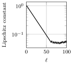
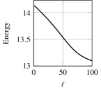
(a)	(b)

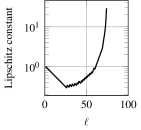
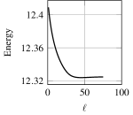
Figure 2: The Cat experiment, $k=1$: (a) local Lipschitz constants obtained by the lazy backtracking strategy; (b) objective function $f+g$ as a function of the iPiano iterations count $\ell$.

(a)	(b)

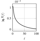
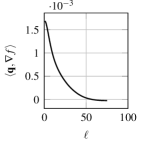
Figure 3: The Cat experiment, $k=2$: (a) local Lipschitz constants obtained by the lazy-backtracking strategy. At $\ell=75$ the increase generates a small $\alpha^{(\ell)}$, therefore the iPiano break criteria is fulfilled; (b) objective function $f+g$ as a function of the iPiano iterations count $\ell$. Starting at $\ell=46$ the objective function slightly increases. This is not contrary to the convergence theory, since the descent property is fulfilled for a majorising sequence.

(a)	(b)

Figure 4: The Cat experiment: $\langle\textbf{q},\nabla f\rangle$ for (a) $k=1$ and (b) $k=2$. For non-negative values the vector $-\vec{q}(\vec{z}^{(\ell)})$ is a descent direction.

We did not observe any spikes in the sequence of local Lipschitz or increasing energies when the exact gradient (43) was used. Therefore the use of the exact gradient would lead to a somehow smoother and faster convergence in terms of number of iterations. However, $\vec{q}(\vec{z})$ can be computed much faster than $\nabla f(\vec{z})$ and we did not observe the exact gradient leading to local minima of (19) with significantly smaller energies, so that we still regard the use of the approximated gradient as the more feasible alternative. In detail, the average computation time (over 100 evaluations) of the exact gradient is roughly 55 seconds, whereas the simplified gradient can be evaluated in 0.13 seconds, which results in a speedup factor of more than 400.

6.2 Numerical results

Figure 5 presents the test data that we use in this paper. It consists of five real-world scenes captured under 20 different known illuminants $\vec{s}^{i}$, ($i=1$, …, $20$), provided in Shi2016 . In our experiments, we used $m=20$ out of the original $96$ RGB images, which we converted to grey levels. Two of the sets present diffuse reflectance (Cat and Pot), while two other exhibit broad specularities (Bear and Buddha) and one presents sparse specular spikes (Ball). Since the ground truth normals are also provided in Shi2016 , the estimated normals can be computed from the final depth map according to (3), and compared to the exact ground truth. For evaluation, we indicate the mean angular error (MAE) (in degrees) over the reconstruction domain $\Omega$.

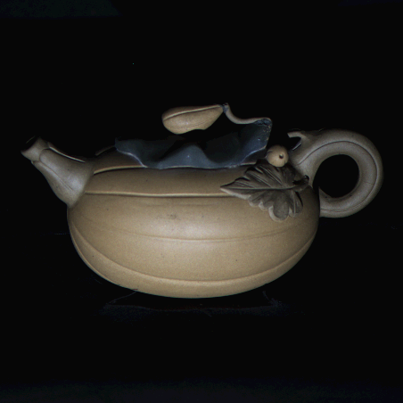
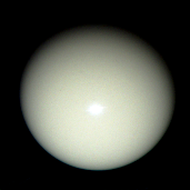
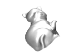
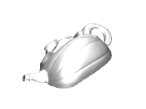
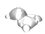
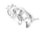
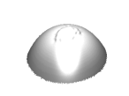
Cat	Pot	Bear	Buddha	Ball

Figure 5: Test data (brightened and cropped to enhance visualisation) and 3D-reconstructions obtained after $500$ iterations $k$ of Algorithm 1.

Let us consider the Cat data set in some detail, as it consists of a diffuse scene that fits rather well our assumptions. We let our algorithm run for $1000$ outer iterations $k$ (approx. $1$ hour on a recent i7 processor, using non-optimised Matlab code), and study the evolution of two criteria: the reprojection error, whose minimum is sought by our algorithm; and the MAE, which indicates the overall accuracy of the 3D reconstruction, c.f. the two left images within Figure 6. The displayed convergence graphs indicate that each iteration from Algorithm 1 not only decreases the value of the objective function $f+g$ (which is approximately equal to the reprojection error $\mathcal{E}_{\mathcal{R}}=f$), but also the MAE. This confirms our conjecture that finding the best possible explanation of the images yields more accurate 3D reconstructions.

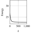
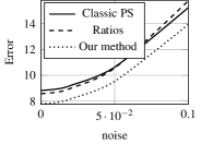
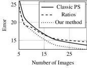
(a)	(b)	(c)	(d)

Figure 6: The Cat experiment: (a) objective function $f+g$ as a function of the iterations count $k$; (b) MAE between the reconstructed surface and the ground truth; (c) reprojection error for competing methods for increasing noise levels (we indicate the standard deviation of the additive, zero-mean Gaussian noise, as a percentage of the maximum intensity); (d) ditto for increasing numbers of input images, with $0.1$ noise level.

In the other two graphs in Figure 6 we study the results of our method compared to other PS strategies based on least-squares: the classical PS framework Woodham1980 consisting in estimating in a least squares sense the normals and the albedo, and integrating them afterwards, and the recent differential ratios procedure from Mecca2016 , forcing Lambertian reflectance and least-squares estimation, for fair comparison. The latter allows direct recovery of the depth, but on the other hand it changes the objective function. Both other approaches rely on linear least squares: they are thus by far faster than the proposed approach (here, a few seconds, versus a few minutes with ours). Yet, in terms of accuracy, these methods are outperformed by our approach, no matter the noise level or the number of images (which were preprocessed via low-rank factorisation Wu2010 in these two experiments).

By making the input images Lambertian via low-rank preprocessing Wu2010 , we can make a reasonable comparison for the whole test dataset. Table 1 shows that our postprocessing method can still improve the accuracy. The 3D reconstruction results obtained with the full pipeline are shown in Figure 7. In comparison with Figure 5, artefacts due to specularities are clearly reduced.

Table 1: Reconstruction errors (MAE, in degrees) obtained for preprocessed input images using the approach from Wu2010 . For fair comparison, the MAE for classic PS is calculated on the final surface, i.e. using the normals calculated by finite differences from the final depth map, rather than the (non-integrable) normals estimated in the first step. Regarding the ratio procedure, we applied the code from Mecca2016 directly on the grey level data.

	Cat	Pot	Bear	Buddha	Ball
Classic PS Woodham1980	8.83	8.92	7.01	14.34	3.05
Differential ratios Mecca2016	8.57	9.00	7.01	14.31	3.13
Our method (500 iter.)	7.79	8.58	6.90	13.89	2.97

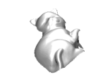
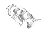
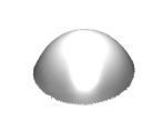
Figure 7: 3D-reconstruction results using the full pipeline, consisting of a preprocessing Wu2010 , followed by classic PS Woodham1980 , and finally the proposed method.

7 Conclusions

We have shown the benefits of recent, high performing numerical methods in the context of photometric stereo. Let us emphasise that only by considering such recent developments in numerical optimisation methods complex models as arising in PS can be handled with success. Our results show that a significant quality gain can be achieved in this way while at the same time the mathematical proceeding can be validated rigorously.

Our experimental investigation has shown what can be expected from the basic iPiano method as well as by computational simplifications as proposed by us in terms of an approximated gradient. In particular we have shown that it may not be easy to interprete relevant properties of computed iterates.

A more detailed view on the computational results reveals that remaining inaccuracies seem to be mostly due to shadows and highlights, edges and depth discontinuities. Thus, an interesting perspective of our work would be to use more robust estimators, which would ensure both robustness to outliers Ikehata2014a ; Queau2017 and improved preservation of edges Durou2009 .

References

- (1) Bähr, M., Breuß, M., Quéau, Y., Boroujerdi, A.S., Durou, J.D.: Fast and accurate surface normal integration on non-rectangular domains. Computational Visual Media 3, 107–129 (2017)
- (2) Bartal, O., Ofir, N., Lipman, Y., Basri, R.: Photometric stereo by hemispherical metric embedding. Journal of Mathematical Imaging and Vision (to appear). URL https://doi.org/10.1007/s10851-017-0748-y
- (3) Basri, R., Jacobs, D., Kemelmacher, I.: Photometric stereo with general, unknown lighting. International Journal of Computer Vision 72, 239–257 (2007)
- (4) Chabrowski, J., Kewei, Z.: On variational approach to photometric stereo. Annales de l’Institut Henri Poincaré (C) Analyse non linéaire 10(4), 363–375 (1993)
- (5) Clark, J.J.: Active photometric stereo. In: IEEE Conference on Computer Vision and Pattern Recognition (CVPR), pp. 29–34 (1992)
- (6) Durou, J.D., Aujol, J.F., Courteille, F.: Integrating the normal field of a surface in the presence of discontinuities. In: Energy Minimization Methods in Computer Vision and Pattern Recognition (EMMCVPR), Lecture Notes in Computer Science, vol. 5681, pp. 261–273. Springer (2009)
- (7) Gotardo, P.F.U., Simon, T., Sheikh, Y., Matthews, I.: Photogeometric scene flow for high-detail dynamic 3D reconstruction. In: Proc. IEEE Int. Conf. Computer Vision (ICCV), pp. 846–854 (2015)
- (8) Harker, M., O’Leary, P.: Regularized reconstruction of a surface from its measured gradient field. Journal of Mathematical Imaging and Vision 51(1), 46–70 (2015)
- (9) Hinkley, D.V.: On the ratio of two correlated normal random variables. Biometrika 56(3), 635–639 (1969)
- (10) Hoeltgen, L., Quéau, Y., Breuß, M., Radow, G.: Optimised photometric stereo via non-convex variational minimisation. In: British Machine Vision Conference (BMVC) (2016). URL https://doi.org/10.5244/C.30.36
- (11) Horn, B.K.P.: Robot Vision. The MIT Press (1986)
- (12) Horn, B.K.P., Woodham, R.J., Silver, W.M.: Determining shape and reflectance using multiple images. Technical Report MIT AITR-490, MIT (1978)
- (13) Horn, R.A., Johnson, C.R.: Topics in Matrix Analysis. Cambridge University Press (1994)
- (14) Ikehata, S., Wipf, D., Matsushita, Y., Aizawa, K.: Photometric stereo using sparse Bayesian regression for general diffuse surfaces. IEEE Transactions on Pattern Analysis and Machine Intelligence 36(9), 1816–1831 (2014)
- (15) Ju, Y.C., Tozza, S., Breuß, M., Bruhn, A., Kleefeld, A.: Generalised perspective shape from shading with Oren-Nayar reflectance. In: British Machine Vision Conference (2013). URL http://doi.org/10.5244/C.27.42
- (16) Khanian, M., Boroujerdi, A.S., Breuß, M.: Photometric stereo for strong specular highlights. Tech. Rep. arXiv:1709.01357 (2017)
- (17) Kozera, R.: Existence and uniqueness in photometric stereo. Aplied Mathematics and Computation 44, 1–103 (1991)
- (18) Lambert, J.H.: Photometria. Klett, Augsburg (1760)
- (19) Magnus, J.R., Neudecker, H.: Matrix differential calculus with applications to simple, Hadamard, and Kronecker products. Journal of Mathematical Psychology 29, 474–492 (1985)
- (20) Magnus, J.R., Neudecker, H.: Matrix Differential Calculus with Applications in Statistics and Econometrics, 3rd edn. John Wiley & Sons (2007)
- (21) Mecca, R., Quéau, Y., Logothetis, F., Cipolla, R.: A single-lobe photometric stereo approach for heterogeneous material. SIAM Journal on Imaging Sciences 9(4), 1858–1888 (2016)
- (22) Mecca, R., Rodolà, E., Cremers, D.: Realistic photometric stereo using partial differential irradiance equation ratios. Computers & Graphics 51, 8–16 (2015)
- (23) Moreau, J.J.: Proximité et dualité dans un espace Hilbertien. Bulletin de la Société Mathématique de France 93, 273–299 (1965)
- (24) Ochs, P.: Unifying abstract inexact convergence theorems for descent methods and block coordinate variable metric iPiano. Tech. rep., Saarland University (2016)
- (25) Ochs, P., Chen, Y., Brox, T., Pock, T.: iPiano: Inertial proximal algorithm for non-convex optimization. SIAM Journal on Imaging Sciences 7(2), 1388–1419 (2014)
- (26) Onn, R., Bruckstein, A.: Integrability disambiguates surface recovery in two-image photometric stereo. International Journal of Computer Vision 5, 105–113 (1990)
- (27) Ortega, J.M., Rheinboldt, W.C.: Iterative Solutions of Nonlinear Equations in Several Variables. New York Academic (1970)
- (28) Papadhimitri, T., Favaro, P.: Uncalibrated near-light photometric stereo. In: British Machine Vision Conference (2014). URL http://doi.org/10.5244/C.28.128
- (29) Petersen, K.B., Pedersen, M.S.: The matrix cookbook (2012). Available from https://www.math.uwaterloo.ca/~hwolkowi/matrixcookbook.pdf
- (30) Pollock, D.S.G.: Tensor products and matrix differential calculus. Linear Algebra and Its Applications 67, 169–193 (1985)
- (31) Quéau, Y., Durix, B., Wu, T., Cremers, D., Lauze, F., Durou, J.D.: LED-based photometric stereo: Modeling, calibration and numerical solution. Journal of Mathematical Imaging and Vision (to appear). URL https://dx.doi.org/10.1007/s10851-017-0761-1
- (32) Quéau, Y., Lauze, F., Durou, J.D.: A -TV algorithm for robust perspective photometric stereo with spatially-varying lightings. In: Scale Space and Variational Methods in Computer Vision (SSVM), Lecture Notes in Computer Science, vol. 9087, pp. 498–510 (2015)
- (33) Quéau, Y., Wu, T., Lauze, F., Durou, J.D., Cremers, D.: A non-convex variational approach to photometric stereo under inaccurate lighting. In: IEEE Conference on Computer Vision and Pattern Recognition (CVPR), pp. 99–108 (2017)
- (34) Reddy, D., Agrawal, A., Chellappa, R.: Enforcing integrability by error correction using -minimization. In: IEEE Conference on Computer Vision and Pattern Recognition (CVPR), pp. 2350–2357 (2009)
- (35) Shi, B., Wu, Z., Mo, Z., Duan, D., Yeung, S.K., Tan, P.: A benchmark dataset and evaluation for non-Lambertian and uncalibrated photometric stereo. In: IEEE Conference on Computer Vision and Pattern Recognition (CVPR), pp. 3707–3716 (2016)
- (36) Smith, W., Fang, F.: Height from photometric ratio with model-based light source selection. Computer Vision and Image Understanding 145, 128–138 (2016)
- (37) Tozza, S., Mecca, R., Duocastella, M., Del Bue, A.: Direct differential photometric stereo shape recovery of diffuse and specular surfaces. Journal of Mathematical Imaging and Vision 56(1), 57–76 (2016)
- (38) Wöhler, C.: 3D Computer Vision. Springer-Verlag (2013)
- (39) Woodham, R.J.: Photometric stereo: A reflectance map technique for determining surface orientation from a single view. In: Proceedings of the 22nd SPIE Annual Technical Symposium, Proceedings of the International Society for Optical Engineering, vol. 155, pp. 136–143 (1978)
- (40) Woodham, R.J.: Photometric method for determining surface orientation from multiple images. Optical Engineering 19(1), 134–144 (1980)
- (41) Wu, L., Ganesh, A., Shi, B., Matsushita, Y., Wang, Y., Ma, Y.: Robust photometric stereo via low-rank matrix completion and recovery. In: Asian Conference on Computer Vision (ACCV), Lecture Notes in Computer Science, vol. 6494, pp. 703–717. Springer Berlin Heidelberg (2010)
- (42) Zeisl, B., Zach, C., Pollefeys, M.: Variational regularization and fusion of surface normal maps. In: IEEE International Conference on 3D Vision (3DV), pp. 601–608 (2014)