Energy-stable linear schemes for polymer-solvent phase field models

Abstract

We present new linear energy-stable numerical schemes for numerical simulation of complex polymer-solvent mixtures. The mathematical model proposed by Zhou, Zhang and E (Physical Review E 73, 2006) consists of the Cahn-Hilliard equation which describes dynamics of the interface that separates polymer and solvent and the Oldroyd-B equations for the hydrodynamics of polymeric mixtures. The model is thermodynamically consistent and dissipates free energy. Our main goal in this paper is to derive numerical schemes for the polymer-solvent mixture model that are energy dissipative and efficient in time. To this end we will propose several problem-suited time discretizations yielding linear schemes and discuss their properties.

1 Introduction

Phase separation in binary fluids is a fundamental process in condensed-matter physics. For Newtonian fluids the phenomenon of spinodal decomposition is reasonably well understood in terms of the so-called “model H” [1, 2, 3], where the hydrodynamic equations of motion for mass and momentum conservation are coupled to a convection-diffusion equation for the concentration (or in general the “phase field” variable $\phi$), and the thermodynamics, which is described by a (free) energy functional $E(\phi)$, gives rise to a driving force, see, e. g., [4, 5, 6, 7]. In such “diffuse interface” or “phase field” models, the interface between two phases is a thin layer of finite thickness, across which $\phi$ varies continuously.

A big advantage of such models is that interfaces are defined implicitly and do not need to be tracked. Similarly, topological changes of the interface structure are automatically described correctly. The physics (and therefore also the mathematics and numerics) becomes more involved if one component — or both — is a macromolecular compound. In this case, the large molecular relaxation time gives rise to a dynamic coupling between intra-molecular processes and the unmixing on experimentally relevant time scales, with interesting new phenomena, for which the term “viscoelastic phase separation” [8] has been coined. Here the construction of physically sound dynamic equations with suitable constitutive relations to describe the viscoelasticity is already a challenge in itself. Tanaka [8] made the first attempt in this direction; however, Zhou et al. [7] showed later that this dynamics violates the second law of thermodynamics and provided a corrected set of equations that satisfy it. We thus study the diffuse-interface viscoelastic equations put forward in [7] for the case of the unmixing process of a polymer-solvent system.

Typically the interfacial region separating the two fluids is very narrow, and a high spatial resolution is required to accurately capture the interface dynamics. In fact, the underlying problem is stiff, which necessitates an implicit time discretization. Moreover, the solution admits several time scales over which it evolves, cf. [9]. In the literature one can find already several numerical methods that have been used for the numerical approximation of diffuse interface models, see, e. g., [10, 6, 9, 11, 5] and the references therein.

In order to describe the dynamics of a complex polymer-solvent mixture, the Cahn-Hilliard equations for the phase field evolution are coupled with the Oldroyd-B equations, which consist of the momentum equation for the velocity field, the continuity equation, and the rheological equation for time evolution of the elastic stress tensor. We note in passing that there is quite a large number of analytical as well as numerical results available in the literature for the Oldroyd-B system, see, e. g., [12, 13, 14, 15]. The main challenge in this field is to obtain a stable approximate numerical solution for large Weissenberg numbers. The dimensionless Weissenberg number represents elastic effects; it is large when the molecular relaxation time is comparable to the time scale of the flow, or even exceeds it significantly. In the present work we consider the non-critical regime of Weissenberg numbers. Applying the techniques from [13, 15], a further generalization using the log-transformation of the elastic stress tensor and the Lagrange-type approximation of the convective term is possible.

The purpose of the present paper is to derive energy-stable and runtime-efficient numerical schemes to solve the above-mentioned equations. This task has already been tackled by us in a preliminary fashion before [16], from which paper we have also taken most of the wording of the present introduction. Compared to Reference [16], we have significantly improved the results, and also provide a much broader context and far more details.

The paper is organized in the following way. In Section 2 we present a mathematical model for the polymer-solvent mixture consisting of the Cahn-Hilliard equation for the interface dynamics and the Oldroyd-B equations for the hydrodynamics. We also introduce a simplified model modelling only interface dynamics of the polymer-solvent mixture without any hydrodynamic effects. Section 3 is devoted to problem-suited numerical methods for both models. We present first and second order schemes that are linear and energy dissipative. We start with numerical methods for the simplified model and continue with corresponding methods for the full model for polymer-solvent mixture. For the latter we propose two types of linear, free energy dissipative schemes, fully coupled schemes in Subsection 3.2 and the splitting scheme in Subsection 3.3. Numerical experiments presented in Section 4 confirm the schemes robustness and reliability to simulate viscoelastic phase separation.

2 Mathematical models

A classical approach to model interface problems is the diffuse interface theory that describes the dynamics of the interfaces by layers of small thickness whose structure is determined by a balance of molecular forces. Here the tendencies for mixing and de-mixing are in competition through a non-local mixing energy. Diffuse interface models are able to treat topological changes of the interface in a natural way. The surface motion is governed by the Cahn-Hilliard equation, see [17], that can be derived as the gradient flow of a phase-field free energy functional

$$E_{mix}(\phi)=\int_{\Omega}\Big{(}\frac{C_{0}}{2}|\nabla\phi|^{2}+F(\phi)\Big{)}\,.$$ (1)

Here $\phi$ denotes the phase-field variable that is used to express the two phases of the system. The phase-field function varies smoothly over the interfacial regions. Further, $\Omega$ is a computational domain with Lipschitz continuous boundary, $C_{0}$ is a positive constant controlling the interface width and $F(\phi)$ denotes a double-well potential that represents the tendency of a system to have two different stable phases.

A simple potential that satisfies these conditions is the Ginzburg-Landau potential

$$F_{pol}(\phi)=\frac{1}{4}(\phi^{2}-1)^{2}\,,$$ (2)

which is defined on the whole real axis, and whose minima occur at $\phi=\pm 1$. This potential is quite often studied in the mathematical literature, see, e. g., Elliot and Zheng [18] or Elliot and Garcke [19, 20]. From a physical point of view, the Flory-Huggins potential [21, 22]

$$F_{log}(\phi)=\frac{1}{n_{p}}\phi\textup{ln}\phi+\frac{1}{n_{s}}(1-\phi)\textup{ln}(1-\phi)+\chi\phi(1-\phi)\,,$$ (3)

which is defined on the interval $(0,1)$ and has two minima within, describes polymer-solvent phase separation more accurately, as it has been derived as a Mean Field theory for polymer systems. In (3), $n_{p}$ and $n_{s}$ denote the degrees of polymerization of the two components, while $\chi>0$ is the (temperature-dependent) Flory-Huggins interaction parameter and we measure the free energy in units of the thermal energy $k_{B}T$, where $k_{B}$ is the Boltzmann constant and $T$ the absolute temperature.

For purposes of the proofs to be presented below, we mostly consider the Ginzburg-Landau potential as defined in (2), however with the modification proposed in, e. g., [23, 24], where the steep increase $\sim\phi^{4}$ outside $[-1,1]$ is replaced by a weaker quadratic rise,

$$\tilde{F}_{pol}=\begin{cases}(\phi+1)^{2}\quad\quad\phi<-1\,,\\ \frac{1}{4}(\phi^{2}-1)^{2}\quad\phi\in[-1,1]\,,\\ (\phi-1)^{2}\quad\quad\phi>1\,.\end{cases}$$ (4)

This modified potential is defined on the whole real axis and has a bounded second derivative. These properties facilitate to establish some bounds needed in the proofs. Thus the Ginzburg-Landau potential allows the derivation of schemes that are energy-stable even though they are linear. It is also possible to derive schemes that are more generally applicable; one of these latter schemes is applied in our numerical experiments, in which we use the Flory-Huggins potential in order to facilitate comparisons with computer simulations of a quasi-atomistic model [16].

Now, the Cahn-Hilliard equation can be derived from the mass balance law

$$\frac{\partial\phi}{\partial t}=-\nabla\cdot J\,,$$

where the mass flux $J$ is defined as

$$J=-m(\phi)\nabla\mu\,.$$

Here

$$m(\phi)=M\left(\phi(1-\phi)\right)^{n}$$

denotes the mobility function with $M$ a positive constant, $n\in\mathbbm{N}_{0}$ and $\mu$ denotes the chemical potential such that

$$\mu:=\frac{\delta E_{mix}}{\delta\phi}=-C_{0}\Delta\phi+f(\phi)\,.$$

Here $\frac{\delta E_{mix}}{\delta\phi}$ is the variational derivative of the mixing energy and $f(\phi)=F^{\prime}(\phi)$.
Gathering this equations yields the Cahn-Hilliard equation

$$\frac{\partial\phi}{\partial t}=\nabla\cdot\Big{\{}M\left(\phi(1-\phi)\right)^{n}\,\nabla\Big{[}-C_{0}\Delta\phi+f(\phi)\Big{]}\Big{\}}\,.$$ (5)

Dynamics of Newtonian two-phase mixtures is usually described as the gradient flow of the free energy consisting of the mixing energy $E_{mix}$ and the kinetic energy $E_{kin}$. This leads to the coupled Cahn-Hilliard-Navier-Stokes system. In order to include the influence of polymers in such a system we extend it to a viscoelastic phase field model. This has been done at first by Tanaka [8] by adding viscoelastic energy due to the bulk and shear stress, here the separation of the total stress tensor into a bulk and a shear part was motivated by Tanaka and Araki [25]. This model violates the second law of thermodynamics, i. e. it is not free energy dissipative. In the recent paper [7] Zhou, Zhang and E propose an improved model for the viscoelastic phase separation that is thermodynamically consistent.

The total free energy $E$ is given as

$$E_{tot}(\phi,q,{\boldsymbol{\sigma}},{\boldsymbol{u}})=E_{mix}(\phi)+E_{kin}({\boldsymbol{u}})+E_{conf}(q)+E_{el}({\boldsymbol{\sigma}})\\ \vskip 6.0pt plus 2.0pt minus 2.0pt\cr=\int_{\Omega}\Big{(}\frac{C_{0}}{2}|\nabla\phi|^{2}+F(\phi)\Big{)}+\int_{\Omega}\frac{1}{2}|{\boldsymbol{u}}|^{2}+\int_{\Omega}\frac{1}{2}|q|^{2}+\int_{\Omega}\frac{1}{2}\textup{tr}({\boldsymbol{\sigma}})\,,$$ (6)

where ${\boldsymbol{u}}$ is the averaged velocity field of the two components, $q$ the scalar bulk stress with $E_{conf}$ the corresponding chain conformational entropy of the polymer molecules and ${\boldsymbol{\sigma}}$ the shear stress tensor with $E_{el}$ the corresponding elastic energy of the polymer molecules. Recalling that the chemical potential $\mu=-C_{0}\Delta\phi+f(\phi)$ and that we work with the Flory-Huggins potential (3), i.e. $\phi\in(0,1)$, we obtain by the variational principle of the free energy minimization following the standard procedures of nonequilibrium thermodynamics, see [7],

$$\frac{\partial\phi}{\partial t}+{\boldsymbol{u}}\cdot\nabla\phi =\nabla\cdot\left\{\phi(1-\phi)\,M\Big{[}\phi(1-\phi)\nabla\mu-\nabla(A_{1}(\phi)\,q)\Big{]}\right\}\,,$$ (7)

$$\frac{\partial q}{\partial t}+{\boldsymbol{u}}\cdot\nabla q =-\frac{1}{\tau_{b}(\phi)}q-A_{1}(\phi)\,\nabla\cdot\left\{M\Big{[}\phi(1-\phi)\nabla\mu-\nabla(A_{1}(\phi)\,q)\Big{]}\right\}\,,$$

$$\frac{\partial{\boldsymbol{\sigma}}}{\partial t}+({\boldsymbol{u}}\cdot\nabla){\boldsymbol{\sigma}} =(\nabla{\boldsymbol{u}})\cdot{\boldsymbol{\sigma}}+{\boldsymbol{\sigma}}\cdot(\nabla{\boldsymbol{u}})^{T}-\frac{1}{\tau_{s}(\phi)}{\boldsymbol{\sigma}}+B_{2}(\phi)\Big{[}\nabla{\boldsymbol{u}}+(\nabla{\boldsymbol{u}})^{T}\Big{]}\,,$$

$$\frac{\partial{\boldsymbol{u}}}{\partial t}+({\boldsymbol{u}}\cdot\nabla){\boldsymbol{u}} =-\nabla p+\nabla\cdot\left\{\eta(\phi)\Big{[}\nabla{\boldsymbol{u}}+(\nabla{\boldsymbol{u}})^{T}\Big{]}\right\}-\nabla\cdot(C_{0}\nabla\phi\otimes\nabla\phi)+\nabla\cdot{\boldsymbol{\sigma}}\,,$$

$$\nabla\cdot{\boldsymbol{u}} =0\,,$$

where $\tau_{b}(\phi)=\tau_{b}^{0}\,\phi^{2}$ and $\tau_{s}(\phi)=\tau_{s}^{0}\,\phi^{2}$ are the relaxation times, $B_{2}(\phi)=m^{0}_{s}\,\phi^{2}$ is the relaxation modulus, and $\tau_{b}^{0},\tau_{s}^{0}$ and $m^{0}_{s}$ are positive constants. $A_{1}(\phi)$ is the bulk modulus. The precise definition will be given in Section 4. Further, $\eta(\phi)=1-\tau_{s}(\phi)B_{2}(\phi)$ is the viscosity which is dependent on the relaxation and $p$ is the pressure. For the aforementioned mobility the quartic function $m(\phi)=M\left(\phi(1-\phi)\right)^{2}$ is used.
Zhou et al. [7] also considered the special case of model (7) without hydrodynamic transport, i. e. ${\boldsymbol{u}}=0$. Note, that we use the same symbol $0$ for a scalar, a vector or a matrix. The resulting simplified model reads

$$\begin{array}[]{c}\displaystyle\frac{\partial\phi}{\partial t}=\nabla\cdot\left\{\phi(1-\phi)M\Big{[}\phi(1-\phi)\nabla\mu-\nabla(A_{1}(\phi)\,q)\Big{]}\right\}\,,\\ \vskip 6.0pt plus 2.0pt minus 2.0pt\cr\displaystyle\frac{\partial q}{\partial t}=-\frac{1}{\tau_{b}(\phi)}q-A_{1}(\phi)\nabla\cdot\left\{M\Big{[}\phi(1-\phi)\nabla\mu-\nabla(A_{1}(\phi)\,q)\Big{]}\,\right..\end{array}$$ (8)

In literature we can find already several well-established numerical methods for the Cahn-Hilliard equation (5), see, e. g., [10, 6, 9, 11, 5]. In order to understand the crucial properties of the viscoelastic two-phase model (7) we start by discussing its simplified version (8) in the following subsection. For the sake of simplicity we will call model (7) the full model and its simplification (8) the simplified model.

2.1 Simplified model (without hydrodynamics)

In a special case when the hydrodynamics effects are neglected, i. e. ${\boldsymbol{u}}=0$, the total energy of the system consists of the mixing energy and the chain conformational energy

$$E_{tot}(\phi,q)=E_{mix}(\phi)+E_{conf}(q)=\int_{\Omega}\Big{(}\frac{C_{0}}{2}|\nabla\phi|^{2}+F(\phi)\Big{)}+\int_{\Omega}\frac{1}{2}|q|^{2}\,.$$ (9)

The minimization principle yields the simplified model (8).

Theorem 2.1.

The problem (8) satisfies the following energy law

$$\frac{dE_{tot}(\phi,q)}{dt}=-\frac{1}{\tau^{0}_{b}}\left\|\frac{q}{\phi}\right\|^{2}_{L^{2}(\Omega)}-\int_{\Omega}M\Big{[}\phi(1-\phi)\nabla\mu-\nabla(A_{1}(\phi)\,q)\Big{]}^{2}\,.$$ (10)

Proof.

Multiplying (8)₁ by $\mu$ and integrating over the computational domain $\Omega$, assuming suitable boundary conditions (e. g. periodic boundary conditions), and applying integration by parts we obtain

$$\begin{array}[]{cl}\displaystyle\hfil&\displaystyle\int_{\Omega}\frac{\partial\phi}{\partial t}\mu-\int_{\Omega}\nabla\cdot\left\{\phi(1-\phi)M\Big{[}\phi(1-\phi)\nabla\mu-\nabla(A_{1}(\phi)\,q)\Big{]}\right\}\mu\\ \vskip 6.0pt plus 2.0pt minus 2.0pt\cr\displaystyle=&\displaystyle\int_{\Omega}\frac{\partial\phi}{\partial t}\frac{\delta E_{mix}(\phi)}{\delta\phi}+\int_{\Omega}\left\{\phi(1-\phi)M\Big{[}\phi(1-\phi)\nabla\mu-\nabla(A_{1}(\phi)\,q)\Big{]}\right\}\nabla\mu\\ \vskip 6.0pt plus 2.0pt minus 2.0pt\cr\displaystyle=&\displaystyle\frac{dE_{mix}(\phi)}{dt}+\int_{\Omega}M\Big{[}\phi(1-\phi)\nabla\mu-\nabla(A_{1}(\phi)\,q)\Big{]}\Big{[}\phi(1-\phi)\nabla\mu\Big{]}=0\,.\end{array}$$

Further, multiplying (8)₂ by $q$ and integrating over $\Omega$ with suitable boundary conditions yields

$$\begin{array}[]{cl}\displaystyle\hfil&\displaystyle\int_{\Omega}\frac{\partial q}{\partial t}q+\int_{\Omega}\frac{1}{\tau_{b}(\phi)}q^{2}+\int_{\Omega}A_{1}(\phi)\nabla\cdot\left\{M\Big{[}\phi(1-\phi)\nabla\mu-\nabla(A_{1}(\phi)\,q)\Big{]}\right\}q\\ \vskip 6.0pt plus 2.0pt minus 2.0pt\cr\displaystyle=&\displaystyle\int_{\Omega}\frac{1}{2}\frac{\partial q^{2}}{\partial t}+\int_{\Omega}\frac{1}{\tau^{0}_{b}\phi^{2}}q^{2}+\int_{\Omega}\nabla\cdot M\Big{[}\phi(1-\phi)\nabla\mu-\nabla(A_{1}(\phi)\,q)\Big{]}A_{1}(\phi)\,q\\ \vskip 6.0pt plus 2.0pt minus 2.0pt\cr\displaystyle=&\displaystyle\frac{d}{dt}\left(\int_{\Omega}\frac{1}{2}q^{2}\right)+\frac{1}{\tau^{0}_{b}}\int_{\Omega}\left(\frac{q}{\phi}\right)^{2}\\ \vskip 6.0pt plus 2.0pt minus 2.0pt\cr\displaystyle\hfil&\displaystyle-\int_{\Omega}M\Big{[}\phi(1-\phi)\nabla\mu-\nabla(A_{1}(\phi)\,q)\Big{]}\nabla(A_{1}(\phi)\,q)\\ \vskip 6.0pt plus 2.0pt minus 2.0pt\cr\displaystyle=&\displaystyle\frac{dE_{conf}(q)}{dt}+\frac{1}{\tau^{0}_{b}}\left\|\frac{q}{\phi}\right\|^{2}_{L^{2}(\Omega)}\\ \vskip 6.0pt plus 2.0pt minus 2.0pt\cr\displaystyle\hfil&\displaystyle+\int_{\Omega}M\Big{[}\phi(1-\phi)\nabla\mu-\nabla(A_{1}(\phi)\,q)\Big{]}\Big{[}-\nabla(A_{1}(\phi)\,q)\Big{]}=0\,.\end{array}$$

Then, adding both relations we obtain

$$\frac{dE_{mix}(\phi)}{dt}+\frac{dE_{conf}(q)}{dt}+\frac{1}{\tau^{0}_{b}}\left\|\frac{q}{\phi}\right\|^{2}_{L^{2}(\Omega)}\\ \vskip 6.0pt plus 2.0pt minus 2.0pt\cr+\int_{\Omega}M\Big{[}\phi(1-\phi)\nabla\mu-\nabla(A_{1}(\phi)\,q)\Big{]}\Big{[}\phi(1-\phi)\nabla\mu-\nabla(A_{1}(\phi)\,q)\Big{]}=0\,,$$

which is the desired energy law (10). ∎

2.2 Full model (with hydrodynamics)

In this Subsection we consider the full two-phase model for viscoelastic phase separation (7). The total free energy of the system consists of the mixing energy, the conformation energy, the elastic energy and the kinetic energy

$$E_{tot}(\phi,q,{\boldsymbol{\sigma}},{\boldsymbol{u}})=E_{mix}(\phi)+E_{conf}(q)+E_{el}({\boldsymbol{\sigma}})+E_{kin}({\boldsymbol{u}})\\ \vskip 6.0pt plus 2.0pt minus 2.0pt\cr=\int_{\Omega}\Big{(}\frac{C_{0}}{2}|\nabla\phi|^{2}+F(\phi)\Big{)}+\int_{\Omega}\frac{1}{2}|q|^{2}+\int_{\Omega}\frac{1}{2}\textup{tr}({\boldsymbol{\sigma}})+\int_{\Omega}\frac{1}{2}|{\boldsymbol{u}}|^{2}\,.$$ (11)

In order to prove that a solution of (7) dissipates the total free energy in time we need the following lemma.

Lemma 2.1.

The following relation holds

$$\nabla\cdot(C_{0}\nabla\phi\otimes\nabla\phi)=-\mu\nabla\phi+\nabla\left(\frac{C_{0}}{2}|\nabla\phi|^{2}+F(\phi)\right)\,.$$ (12)

Proof.

For $e_{i}$ the $i$-th unit vector and $d$ the spatial dimension the following relation holds

$$\begin{array}[]{l}\displaystyle\nabla\cdot(C_{0}\nabla\phi\otimes\nabla\phi)=C_{0}\sum_{j=1}^{d}\frac{\partial}{\partial x_{j}}\left(\sum_{i=1}^{d}\frac{\partial\phi}{\partial x_{i}}e_{i}\cdot\sum_{j=1}^{d}\frac{\partial\phi}{\partial x_{j}}e_{j}^{T}\right)\\ \vskip 6.0pt plus 2.0pt minus 2.0pt\cr\displaystyle=C_{0}\sum_{i,j=1}^{d}\frac{\partial}{\partial x_{j}}\left(\frac{\partial\phi}{\partial x_{i}}\frac{\partial\phi}{\partial x_{j}}\right)e_{i}=C_{0}\sum_{i,j=1}^{d}\left(\frac{\partial\phi}{\partial x_{i}}\frac{\partial^{2}\phi}{\partial x_{j}^{2}}+\frac{\partial^{2}\phi}{\partial x_{i}\partial x_{j}}\frac{\partial\phi}{\partial x_{j}}\right)e_{i}\\ \vskip 6.0pt plus 2.0pt minus 2.0pt\cr\displaystyle=C_{0}\sum_{j=1}^{d}\frac{\partial^{2}\phi}{\partial x_{j}^{2}}\cdot\sum_{i=1}^{d}\frac{\partial\phi}{\partial x_{i}}e_{i}+\frac{C_{0}}{2}\sum_{i=1}^{d}\frac{\partial}{\partial x_{i}}\sum_{j=1}^{d}\left(\frac{\partial\phi}{\partial x_{j}}\right)^{2}e_{i}\\ \vskip 6.0pt plus 2.0pt minus 2.0pt\cr\displaystyle=C_{0}\sum_{j=1}^{d}\frac{\partial^{2}\phi}{\partial x_{j}^{2}}\cdot\sum_{i=1}^{d}\frac{\partial\phi}{\partial x_{i}}e_{i}+\frac{C_{0}}{2}\sum_{i=1}^{d}\frac{\partial}{\partial x_{i}}\sum_{j=1}^{d}\left(\frac{\partial\phi}{\partial x_{j}}\right)^{2}e_{i}+\left(\frac{\partial F(\phi)}{\partial\phi}-f(\phi)\right)\frac{\partial\phi}{\partial x_{i}}e_{i}\\ \vskip 6.0pt plus 2.0pt minus 2.0pt\cr\displaystyle=\left(C_{0}\sum_{j=1}^{d}\frac{\partial^{2}\phi}{\partial x_{j}^{2}}-f(\phi)\right)\sum_{i=1}^{d}\frac{\partial\phi}{\partial x_{i}}e_{i}+\sum_{i=1}^{d}\frac{\partial}{\partial x_{i}}e_{i}\left(\frac{C_{0}}{2}\sum_{j=1}^{d}\left(\frac{\partial\phi}{\partial x_{j}}\right)^{2}+F(\phi)\right)\\ \vskip 6.0pt plus 2.0pt minus 2.0pt\cr\displaystyle=\big{(}C_{0}\Delta\phi-f(\phi)\big{)}\nabla\phi+\nabla\left(\frac{C_{0}}{2}|\nabla\phi|^{2}+F(\phi)\right)\\ \vskip 6.0pt plus 2.0pt minus 2.0pt\cr\displaystyle=-\mu\nabla\phi+\nabla\Big{(}\frac{C_{0}}{2}|\nabla\phi|^{2}+F(\phi)\Big{)}\,.\end{array}$$

∎

Now, we introduce the new pressure term $\tilde{p}=p+\frac{C_{0}}{2}|\nabla\phi|^{2}+F(\phi)$. Together with equation (12) this allows us to rewrite system (7) as follows

$$\frac{\partial\phi}{\partial t}+{\boldsymbol{u}}\cdot\nabla\phi -\nabla\cdot\left\{\phi(1-\phi)M\Big{[}\phi(1-\phi)\nabla\mu-\nabla(A_{1}(\phi)\,q)\Big{]}\right\}=0\,,$$ (13)

$$\frac{\partial q}{\partial t}+{\boldsymbol{u}}\cdot\nabla q +\frac{1}{\tau_{b}(\phi)}q+A_{1}(\phi)\nabla\cdot\left\{M\Big{[}\phi(1-\phi)\nabla\mu-\nabla(A_{1}(\phi)\,q)\Big{]}\right\}=0\,,$$

$$\frac{\partial{\boldsymbol{\sigma}}}{\partial t}+({\boldsymbol{u}}\cdot\nabla){\boldsymbol{\sigma}} -(\nabla{\boldsymbol{u}})\cdot{\boldsymbol{\sigma}}-{\boldsymbol{\sigma}}\cdot(\nabla{\boldsymbol{u}})^{T}+\frac{1}{\tau_{s}(\phi)}{\boldsymbol{\sigma}}-B_{2}(\phi)\Big{[}\nabla{\boldsymbol{u}}+(\nabla{\boldsymbol{u}})^{T}\Big{]}=0\,,$$

$$\frac{\partial{\boldsymbol{u}}}{\partial t}+({\boldsymbol{u}}\cdot\nabla){\boldsymbol{u}} -\nabla\cdot\left\{\eta(\phi)\Big{[}\nabla{\boldsymbol{u}}+(\nabla{\boldsymbol{u}})^{T}\Big{]}\right\}+\nabla\tilde{p}-\mu\nabla\phi-\nabla\cdot{\boldsymbol{\sigma}}=0\,,$$

$$\nabla\cdot{\boldsymbol{u}} =0\,.$$

Theorem 2.2.

System (13) obeys the following energy law

$$\frac{dE_{tot}(\phi,q,{\boldsymbol{\sigma}},{\boldsymbol{u}})}{dt}=-\frac{1}{\tau^{0}_{b}}\left\|\frac{q}{\phi}\right\|^{2}_{L^{2}(\Omega)}-\int_{\Omega}M\Big{[}\phi(1-\phi)\nabla\mu-\nabla(A_{1}(\phi)\,q)\Big{]}^{2}\\ \vskip 6.0pt plus 2.0pt minus 2.0pt\cr-\int_{\Omega}\frac{1}{2\,\tau_{s}(\phi)}\textup{tr}({\boldsymbol{\sigma}})-\int_{\Omega}\frac{\eta(\phi)}{2}\sum_{i,j=1}^{d}\left(\frac{\partial u_{i}}{\partial x_{j}}+\frac{\partial u_{j}}{\partial x_{i}}\right)^{2}\,.$$ (14)

Proof.

Analogously to the derivation of the energy law (10), $\eqref{eq:model3}_{1}$ is multiplied by $\mu$ and (13)₂ by $q$ and both are integrated. Assuming suitable boundary conditions we obtain

$$\frac{dE_{mix}(\phi)}{dt}+\frac{dE_{conf}(q)}{dt}+\frac{1}{\tau^{0}_{b}}\left\|\frac{q}{\phi}\right\|^{2}_{L^{2}(\Omega)}\\ +\int_{\Omega}M\Big{[}\phi(1-\phi)\nabla\mu-\nabla(A_{1}(\phi)\,q)\Big{]}^{2}+\int_{\Omega}{\boldsymbol{u}}\cdot\nabla\phi\mu=0\,.$$

Further, we multiply (13)₃ by $\frac{1}{2}\mathbbm{1}$, where $\mathbbm{1}$ is the unit matrix, and integrate over $\Omega$. Taking into account that for all $\textbf{A}\in\mathbbm{R}^{n\times n},n\in\mathbbm{N},\textbf{A}:\mathbbm{1}=\textup{tr}(\textbf{A}\cdot\mathbbm{1})=\textup{tr}(\textbf{A})$ we get

$$\int_{\Omega}\frac{1}{2}\textup{tr}\left(\frac{\partial{\boldsymbol{\sigma}}}{\partial t}\right)+\int_{\Omega}\frac{1}{2}\textup{tr}\left(({\boldsymbol{u}}\cdot\nabla){\boldsymbol{\sigma}}\right)-\int_{\Omega}\frac{1}{2}\left(\nabla{\boldsymbol{u}}:{\boldsymbol{\sigma}}^{T}+{\boldsymbol{\sigma}}:\nabla{\boldsymbol{u}}\right)$$

$$-\int_{\Omega}\frac{1}{2\,\tau_{s}(\phi)}\textup{tr}({\boldsymbol{\sigma}})+B_{2}(\phi)\textup{tr}(\nabla{\boldsymbol{u}})$$

$$=\quad \int_{\Omega}\frac{1}{2}\frac{\partial\,\textup{tr}({\boldsymbol{\sigma}})}{\partial t}-\int_{\Omega}\frac{1}{2}\textup{tr}\left((\nabla\cdot{\boldsymbol{u}}){\boldsymbol{\sigma}}\right)-\int_{\Omega}{\boldsymbol{\sigma}}:\nabla{\boldsymbol{u}}$$

$$+\int_{\Omega}\frac{1}{2\,\tau_{s}(\phi)}\textup{tr}({\boldsymbol{\sigma}})+\int_{\Omega}B_{2}(\phi)(\nabla\cdot{\boldsymbol{u}})$$

$$=\quad \frac{d}{dt}\int_{\Omega}\frac{1}{2}\textup{tr}({\boldsymbol{\sigma}})-\int_{\Omega}{\boldsymbol{\sigma}}:\nabla{\boldsymbol{u}}+\int_{\Omega}\frac{1}{2\,\tau_{s}(\phi)}\textup{tr}({\boldsymbol{\sigma}})=0\,.$$

Multiplying $\eqref{eq:model3}_{4}$ by ${\boldsymbol{u}}$ and integrating over $\Omega$ yields

$$\int_{\Omega}\frac{\partial{\boldsymbol{u}}}{\partial t}\cdot{\boldsymbol{u}}+\int_{\Omega}({\boldsymbol{u}}\cdot\nabla)|{\boldsymbol{u}}|^{2}+\int_{\Omega}\left\{\eta(\phi)\Big{[}\nabla{\boldsymbol{u}}+(\nabla{\boldsymbol{u}})^{T}\Big{]}\right\}:\nabla{\boldsymbol{u}}$$

$$-\int_{\Omega}\tilde{p}(\nabla\cdot{\boldsymbol{u}})-\mu\nabla\phi\cdot{\boldsymbol{u}}+\nabla\cdot{\boldsymbol{\sigma}}\cdot{\boldsymbol{u}}$$

$$=\quad \int_{\Omega}\frac{1}{2}\frac{\partial|{\boldsymbol{u}}|^{2}}{\partial t}-\int_{\Omega}(\nabla\cdot{\boldsymbol{u}})|{\boldsymbol{u}}|^{2}+\int_{\Omega}\left\{\eta(\phi)\Big{[}|\nabla{\boldsymbol{u}}|^{2}+Tr\left((\nabla{\boldsymbol{u}})^{2}\right)\Big{]}\right\}$$

$$-\int_{\Omega}{\boldsymbol{u}}\cdot\nabla\phi\mu+\int_{\Omega}{\boldsymbol{\sigma}}:\nabla{\boldsymbol{u}}$$

$$=\quad \frac{d}{dt}\int_{\Omega}\frac{1}{2}|{\boldsymbol{u}}|^{2}+\int_{\Omega}\frac{\eta(\phi)}{2}\sum_{i,j=1}^{d}\left(\frac{\partial u_{i}}{\partial x_{j}}+\frac{\partial u_{j}}{\partial x_{i}}\right)^{2}-\int_{\Omega}{\boldsymbol{u}}\cdot\nabla\phi\mu+\int_{\Omega}{\boldsymbol{\sigma}}:\nabla{\boldsymbol{u}}=0\,.$$

Summing up the above relations we obtain the energy law (14). ∎

Remark 2.1.

We should point out that the elastic stress tensor ${\boldsymbol{\sigma}}$ does not necessarily need to be positive definite. Thus, $tr({\boldsymbol{\sigma}})$ in the energy law (14) is not necessarily positive and could therefore interfere with the energy dissipation. To control this we introduce the so-called conformation tensor ${\boldsymbol{c}}$, ${\boldsymbol{c}}:=\frac{1}{B_{2}(\phi)}{\boldsymbol{\sigma}}+\mathbbm{1}$, where $\mathbbm{1}$ is the identity matrix. By its definition the conformation tensor ${\boldsymbol{c}}$ is positive definite. In [26] Hu and Lelièvre studied the classical Oldroyd-B model with $B_{2}(\phi)=$ const. and $\tau_{s}(\phi)=$ const. They were able to prove that if the determinant of the initial conformation tensor is greater than one, then $\textup{tr}({\boldsymbol{\sigma}})>0$ for all times. This result indicates that it is important to control the initial data for the elastic stress ${\boldsymbol{\sigma}}$ in such a way that the determinant of ${\boldsymbol{c}}$ is enough large in order to get an elastic stress tensor which remains positive definite as well.

Remark 2.2.

Since the full model is incompressible, it holds $\nabla\cdot({\boldsymbol{u}}w)={\boldsymbol{u}}\cdot\nabla w+\nabla\cdot{\boldsymbol{u}}w={\boldsymbol{u}}\cdot\nabla w,\ \ w\in\{\phi,q\},$ for the advection terms, allowing us to rewrite model (13) as follows

$$\begin{array}[]{l}\displaystyle\frac{\partial\phi}{\partial t}+\nabla\cdot({\boldsymbol{u}}\phi)-\nabla\cdot\left\{\phi(1-\phi)M\Big{[}\phi(1-\phi)\nabla\mu-\nabla(A_{1}(\phi)\,q)\Big{]}\right\}=0\,,\\ \vskip 6.0pt plus 2.0pt minus 2.0pt\cr\displaystyle\frac{\partial q}{\partial t}+\nabla\cdot({\boldsymbol{u}}q)+\frac{1}{\tau_{b}(\phi)}q+A_{1}(\phi)\nabla\cdot\left\{M\Big{[}\phi(1-\phi)\nabla\mu-\nabla(A_{1}(\phi)\,q)\Big{]}\right\}=0\,,\\ \vskip 6.0pt plus 2.0pt minus 2.0pt\cr\displaystyle\frac{\partial{\boldsymbol{\sigma}}}{\partial t}+({\boldsymbol{u}}\cdot\nabla){\boldsymbol{\sigma}}-(\nabla{\boldsymbol{u}})\cdot{\boldsymbol{\sigma}}-{\boldsymbol{\sigma}}\cdot(\nabla{\boldsymbol{u}})^{T}+\frac{1}{\tau_{s}(\phi)}{\boldsymbol{\sigma}}-B_{2}(\phi)\Big{[}\nabla{\boldsymbol{u}}+(\nabla{\boldsymbol{u}})^{T}\Big{]}=0\,,\\ \vskip 6.0pt plus 2.0pt minus 2.0pt\cr\displaystyle\frac{\partial{\boldsymbol{u}}}{\partial t}+({\boldsymbol{u}}\cdot\nabla){\boldsymbol{u}}-\nabla\cdot\left\{\eta(\phi)\Big{[}\nabla{\boldsymbol{u}}+(\nabla{\boldsymbol{u}})^{T}\Big{]}\right\}+\nabla\hat{p}+\phi\nabla\mu-\nabla\cdot{\boldsymbol{\sigma}}=0\,,\\ \vskip 6.0pt plus 2.0pt minus 2.0pt\cr\displaystyle\quad\nabla\cdot{\boldsymbol{u}}=0\,,\end{array}$$ (15)

where the pressure term $\hat{p}=\tilde{p}-\phi\mu$. This model will be useful for our new splitting scheme in Subsection 3.3.

In what follows we will write for the sake of simplicity $p$ instead of $\tilde{p}$ and $\hat{p}$.

3 Numerical schemes

3.1 Schemes for the simplified model

We start this Subsection proposing the one step numerical scheme for the simplified model (8). We consider an uniform partition of the time interval $[0,T]$ with a constant time step $\Delta t$. Given $(\phi^{n},q^{n})$ from the previous time step we compute $(\phi^{n+1},q^{n+1})$ such that

$$\frac{\phi^{n+1}-\phi^{n}}{\Delta t} -\nabla\cdot\left\{\phi^{n}(1-\phi^{n})M\Big{[}\phi^{n}(1-\phi^{n})\nabla\mu^{n+\frac{1}{2}}-\nabla(A_{1}(\phi^{n})\,q^{n+\frac{1}{2}})\Big{]}\right\}=0\,,$$ (16)

$$\frac{q^{n+1}-q^{n}}{\Delta t} +\frac{1}{\tau_{b}(\phi^{n})}q^{n+\frac{1}{2}}$$

$$\quad\ \ +A_{1}(\phi^{n})\nabla\cdot\left\{M\Big{[}\phi^{n}(1-\phi^{n})\nabla\mu^{n+\frac{1}{2}}-\nabla(A_{1}(\phi^{n})\,q^{n+\frac{1}{2}})\Big{]}\right\}=0\,,$$

where

$$\mu^{n+\frac{1}{2}}=-C_{0}\Delta\phi^{n+\frac{1}{2}}+f(\phi^{n+1},\phi^{n})\,.$$

Here we use the notations $\phi^{n+\frac{1}{2}}:=\frac{\phi^{n+1}+\phi^{n}}{2}$ and $q^{n+\frac{1}{2}}:=\frac{q^{n+1}+q^{n}}{2}$ that are the Crank-Nicolson-type approximations.

Theorem 3.1.

Let $f(\phi^{n+1},\phi^{n})$ represent a suitable linearized approximation of $f(\phi)=F^{\prime}(\phi)$. Then the resulting numerical scheme (16) is linear and satisfies the following discrete version of the energy law (10)

$$\frac{E_{tot}(\phi^{n+1},q^{n+1})-E_{tot}(\phi^{n},q^{n})}{\Delta t}=-ND^{n+1}_{phobic}-\frac{1}{\tau^{0}_{b}}\left\|\frac{q^{n+\frac{1}{2}}}{\phi^{n}}\right\|^{2}_{L^{2}(\Omega)}\\ \vskip 6.0pt plus 2.0pt minus 2.0pt\cr-\int_{\Omega}M\Big{[}\phi^{n}(1-\phi^{n})\nabla\mu^{n+\frac{1}{2}}-\nabla(A_{1}(\phi^{n})\,q^{n+\frac{1}{2}})\Big{]}^{2}\,,$$ (17)

where

$$ND^{n+1}_{phobic}:=\int_{\Omega}f(\phi^{n+1},\phi^{n})\frac{\phi^{n+1}-\phi^{n}}{\Delta t}-\int_{\Omega}\frac{F(\phi^{n+1})-F(\phi^{n})}{\Delta t}\,.$$

Depending on the approximation considered for $f(\phi^{n+1},\phi^{n})$, we obtain different numerical schemes with different discrete energy laws, see Remark 3.1.

Proof.

It is clear that the proposed scheme is linear. The discrete mixing and conformation energy can be derived following the same calculations presented in the proof of Theorem 2.1. Multiplying (16)₁ by $\mu^{n+\frac{1}{2}}$, integrating over $\Omega$ and applying suitable boundary conditions yields

$$\frac{E_{mix}(\phi^{n+1})-E_{mix}(\phi^{n})}{\Delta t}+ND^{n+1}_{phobic}\\ \vskip 6.0pt plus 2.0pt minus 2.0pt\cr+\int_{\Omega}M\Big{[}\phi^{n}(1-\phi^{n})\nabla\mu^{n+\frac{1}{2}}-\nabla(A_{1}(\phi^{n})\,q^{n+\frac{1}{2}})\Big{]}\Big{[}\phi^{n}(1-\phi^{n})\nabla\mu^{n+\frac{1}{2}}\Big{]}=0\,.$$

Analogously, multiplying (16)₂ by $q^{n+\frac{1}{2}}$, integrating over $\Omega$ while assuming suitable boundary conditions implies

$$\frac{E_{conf}(q^{n+1})-E_{conf}(q^{n})}{\Delta t}+\frac{1}{\tau^{0}_{b}}\left\|\frac{q^{n+\frac{1}{2}}}{\phi^{n}}\right\|^{2}_{L^{2}(\Omega)}\\ \vskip 6.0pt plus 2.0pt minus 2.0pt\cr+\int_{\Omega}M\Big{[}\phi^{n}(1-\phi^{n})\nabla\mu^{n+\frac{1}{2}}-\nabla(A_{1}(\phi^{n})\,q^{n+\frac{1}{2}})\Big{]}\Big{[}-\nabla(A_{1}(\phi^{n})q^{n+\frac{1}{2}})\Big{]}=0\,.$$

Summing up both relations leads to the discrete energy conservation law (17). ∎

The numerical scheme (16) is linear and first order in time. We propose a linear second order numerical scheme by using a second order extrapolation for the explicit terms, arriving at a two-step numerical scheme, obeying an analogous discrete energy law as scheme (16). The proposed linear second order numerical scheme reads

$$\frac{\phi^{n+1}-\phi^{n}}{\Delta t}$$ (18)

$$- \nabla\cdot\left\{\phi^{n-\frac{1}{2}}(1-\phi^{n-\frac{1}{2}})M\Big{[}\phi^{n-\frac{1}{2}}(1-\phi^{n-\frac{1}{2}})\nabla\mu^{n+\frac{1}{2}}-\nabla(A_{1}(\phi^{n-\frac{1}{2}})\,q^{n+\frac{1}{2}})\Big{]}\right\}=0\,,$$

$$\frac{q^{n+1}-q^{n}}{\Delta t}+\frac{1}{\tau_{b}(\phi^{n-\frac{1}{2}})}q^{n+\frac{1}{2}}$$

$$\quad+A_{1}(\phi^{n-\frac{1}{2}})\nabla\cdot\left\{M\Big{[}\phi^{n-\frac{1}{2}}(1-\phi^{n-\frac{1}{2}})\nabla\mu^{n+\frac{1}{2}}-\nabla(A_{1}(\phi^{n-\frac{1}{2}})\,q^{n+\frac{1}{2}})\Big{]}\right\}=0\,,$$

where

$$\mu^{n+\frac{1}{2}}=-C_{0}\Delta\phi^{n+\frac{1}{2}}+f(\phi^{n+1},\phi^{n})\,,$$

and

$$\phi^{n-\frac{1}{2}}:=\frac{3\phi^{n}-\phi^{n-1}}{2}$$

is the second order extrapolation at the intermediate old time level $t_{n-1/2}$. In order to compute the pair $(\phi^{1},q^{1})$ from $(\phi^{0},q^{0})$ a second order one-step nonlinear scheme could be considered. We overcome this by setting $\phi^{-1}:=\phi^{0}$ and thus solving the first order scheme in the first time step. As long as the initial data is sufficiently smooth, the influence is usually negligible for $T\gg 0$, see the experimental order of convergence (EOC) presented in Section 4, Table 1.

Definition 3.1.

A numerical scheme is called energy-stable if for any $n\in\mathbbm{N}$

$$E_{tot}(w^{n+1})\leq E_{tot}(w^{n})\,,$$

where $w^{n+1}$ and $w^{n}$ are the solution vectors at times $t_{n+1}$ and $t_{n}$, respectively.

Remark 3.1.

The choice of the approximation for $f(\phi^{n+1},\phi^{n})$ strongly depends on the given potential $F(\phi)$. Anyway, in order to obtain an energy-stable numerical scheme it is necessary that $ND^{n+1}_{phobic}\geq 0$, i. e.

$$\int_{\Omega}f(\phi^{n+1},\phi^{n})\frac{\phi^{n+1}-\phi^{n}}{\Delta t}\geq\int_{\Omega}\frac{F(\phi^{n+1})-F(\phi^{n})}{\Delta t}\,.$$

In the literature the Ginzburg-Landau potential $F_{pol}$ (2) is often used, however with the above-mentioned modification proposed, e. g., by Wu, van Zwieten and van der Zee [23]. This potential $\tilde{F}_{pol}$ (4) has a bounded second derivative,

$$\|f^{\prime}\|_{L^{\infty}(\mathbbm{R})}=\|f^{\prime}\|_{L^{\infty}(-1,1)}=2.$$

For this case we propose to use, following Guillén-González, Rodríguez-Bellido and Tierra [24], the linear first order approximation

$$f_{1}(\phi^{n+1},\phi^{n})=f(\phi^{n})+\frac{1}{2}||f^{\prime}||_{L^{\infty}(\mathbbm{R})}(\phi^{n+1}-\phi^{n})=f(\phi^{n})+\phi^{n+1}-\phi^{n}\,,$$ (19)

which has been shown [24] to satisfy $ND^{n+1}_{phobic}\geq 0$.

For the linear second order approximation we suggest to use the convex-concave splitting of the potential, which has been proposed by Wu et al. [23]. The corresponding approximation for $f(\phi^{n+1},\phi^{n})$ consists of two second order Taylor approximations and reads

$$f_{2}(\phi^{n+1},\phi^{n})= f_{vex}(\phi^{n+1})-\frac{\phi^{n+1}-\phi^{n}}{2}f^{\prime}_{vex}(\phi^{n+1})$$ (20)

$$+f_{cave}(\phi^{n})+\frac{\phi^{n+1}-\phi^{n}}{2}f^{\prime}_{cave}(\phi^{n})\,.$$

Since the convex part reads $f_{vex}=2\phi$, approximation (20) is linear. Note that the derivative of the concave part, $f_{cave}=\phi^{3}-3\phi$, is nonlinear and thus calculated explicitly. Further, to achieve energy stability by using approximation (20), the chemical potential has to be modified in the following way

$$\mu^{n+\frac{1}{2}}= -C_{0}\Delta\phi^{n+\frac{1}{2}}+f_{2}(\phi^{n+1},\phi^{n})$$ (21)

$$-\Delta t\frac{\left(\|f^{\prime}_{vex}\|_{L^{\infty}(-1,1)}+\|-f^{\prime}_{cave}\|_{L^{\infty}(-1,1)}\right)^{2}}{16}\Delta\phi^{n+\frac{1}{2}}\,.$$

We note that the Flory-Huggins potential $F_{log}$ is logarithmic and its derivatives are unbounded. Consequently, the choice of linear approximations for $f(\phi^{n+1},\phi^{n})$ while utilizing this more accurate potential is severely limited. To ensure energy dissipation without modifying the potential, it is necessary to use a nonlinear approximation for $f(\phi^{n+1},\phi^{n})$. Since we are focusing on linear schemes we propose to use the second order Taylor approximation

$$f_{3}(\phi^{n+1},\phi^{n})=f(\phi^{n})+\frac{\phi^{n+1}-\phi^{n}}{2}f^{\prime}(\phi^{n})\,.$$ (22)

This is called the “optimal dissipation 2” (OD2) approximation, see [6], because it leads to $ND^{n+1}_{phobic}=\mathcal{O}(\Delta t^{2})$. However, using this approximation it is not possible to control the sign of $ND^{n+1}_{phobic}$. Nevertheless, our numerical simulations presented in Section 4 suggest that the dissipation of the total energy is not violated.

In the recent work [27] Yang and Zhao have proposed a modification of $F_{log}$ introducing a suitable cut off function close to the boundaries in order to achieve the boundedness of the derivatives. Consequently, we can, e. g., use the above mentioned convex-concave splitting (20) with a modified chemical potential (21). We may thus achieve a linear, second order and provably energy-stable numerical scheme, using a modified Flory-Huggins potential. Verification of this question is left for a future work.

3.2 Coupled schemes for the full model

In this Subsection we present fully coupled linear energy dissipative schemes for the full two-phase model for viscoelastic phase separation (7). Given
$(\phi^{n},q^{n},{\boldsymbol{\sigma}}^{n},{\boldsymbol{u}}^{n})$ from the previous time step we compute
$(\phi^{n+1},q^{n+1},{\boldsymbol{\sigma}}^{n+1},{\boldsymbol{u}}^{n+1},p^{n+1})$ such that

$$\frac{\phi^{n+1}-\phi^{n}}{\Delta t} +{\boldsymbol{u}}^{n+1}\cdot\nabla\phi^{n}$$ (23)

$$-\nabla\cdot\left\{\phi^{n}(1-\phi^{n})M\Big{[}\phi^{n}(1-\phi^{n})\nabla\mu^{n+\frac{1}{2}}-\nabla(A_{1}(\phi^{n})\,q^{n+\frac{1}{2}})\Big{]}\right\}=0\,,$$

$$\frac{q^{n+1}-q^{n}}{\Delta t} +{\boldsymbol{u}}^{n}\cdot\nabla q^{n+\frac{1}{2}}+\frac{1}{\tau_{b}(\phi^{n})}q^{n+\frac{1}{2}}$$

$$+A_{1}(\phi^{n})\nabla\cdot\left\{M\Big{[}\phi^{n}(1-\phi^{n})\nabla\mu^{n+\frac{1}{2}}-\nabla(A_{1}(\phi^{n})\,q^{n+\frac{1}{2}})\Big{]}\right\}=0\,,$$

$$\frac{{\boldsymbol{\sigma}}^{n+1}-{\boldsymbol{\sigma}}^{n}}{\Delta t} +({\boldsymbol{u}}^{n}\cdot\nabla){\boldsymbol{\sigma}}^{n}-(\nabla{\boldsymbol{u}}^{n+1})\cdot{\boldsymbol{\sigma}}^{n}-{\boldsymbol{\sigma}}^{n}\cdot\left(\nabla{\boldsymbol{u}}^{n+1}\right)^{T}$$

$$+\frac{1}{\tau_{s}(\phi^{n+\frac{1}{2}})}{\boldsymbol{\sigma}}^{n}-B_{2}(\phi^{n+\frac{1}{2}})\Big{[}\nabla{\boldsymbol{u}}^{n+1}+(\nabla{\boldsymbol{u}}^{n+1})^{T}\Big{]}=0\,,$$

$$\frac{{\boldsymbol{u}}^{n+1}-{\boldsymbol{u}}^{n}}{\Delta t} +({\boldsymbol{u}}^{n}\cdot\nabla){\boldsymbol{u}}^{n+1}-\nabla\cdot\left\{\eta(\phi^{n})\Big{[}\nabla{\boldsymbol{u}}^{n+1}+(\nabla{\boldsymbol{u}}^{n+1})^{T}\Big{]}\right\}$$

$$+\nabla p^{n+1}-\mu^{n+\frac{1}{2}}\nabla\phi^{n}-\nabla\cdot{\boldsymbol{\sigma}}^{n}=0\,,$$

$$\nabla\cdot{\boldsymbol{u}}^{n+1} =0\,,$$

where

$$\mu^{n+\frac{1}{2}}=-C_{0}\Delta\phi^{n+\frac{1}{2}}+f(\phi^{n+1},\phi^{n})\,.$$

Theorem 3.2.

The numerical scheme (23) is linear (up to the approximation considered for $f(\phi^{n+1},\phi^{n})$) and satisfies the discrete version of the energy law (14)

$$\frac{E_{tot}(\phi^{n+1},q^{n+1},{\boldsymbol{\sigma}}^{n+1},{\boldsymbol{u}}^{n+1})-E_{tot}(\phi^{n},q^{n},{\boldsymbol{\sigma}}^{n},{\boldsymbol{u}}^{n})}{\Delta t}=-ND^{n+1}_{phobic}\\ \vskip 6.0pt plus 2.0pt minus 2.0pt\cr-\int_{\Omega}M\Big{[}\phi^{n}(1-\phi^{n})\nabla\mu^{n+\frac{1}{2}}-\nabla(A_{1}(\phi^{n})\,q^{n+\frac{1}{2}})\Big{]}^{2}-\frac{1}{\tau^{0}_{b}}\left\|\frac{q^{n+\frac{1}{2}}}{\phi^{n}}\right\|^{2}_{L^{2}(\Omega)}\\ \vskip 6.0pt plus 2.0pt minus 2.0pt\cr-\int_{\Omega}\frac{1}{2\,\tau_{s}(\phi^{n+\frac{1}{2}})}\textup{tr}({\boldsymbol{\sigma}}^{n})-\frac{1}{2\,\Delta t}\|{\boldsymbol{u}}^{n+1}-{\boldsymbol{u}}^{n}\|^{2}_{L^{2}(\Omega)}\\ \vskip 6.0pt plus 2.0pt minus 2.0pt\cr-\int_{\Omega}\frac{\eta(\phi^{n})}{2}\sum_{i,j=1}^{d}\left(\frac{\partial u^{n+1}_{i}}{\partial x_{j}}+\frac{\partial u^{n+1}_{j}}{\partial x_{i}}\right)^{2}\,,$$ (24)

where

$$ND^{n+1}_{phobic}:=\int_{\Omega}f(\phi^{n+1},\phi^{n})\frac{\phi^{n+1}-\phi^{n}}{\Delta t}-\int_{\Omega}\frac{F(\phi^{n+1})-F(\phi^{n})}{\Delta t}\,.$$

Proof.

Analogously to the derivation of the discrete energy law (17), (23)₁ is multiplied by $\mu^{n+\frac{1}{2}}$ and (23)₂ by $q^{n+\frac{1}{2}}$. Integrating both equations over $\Omega$ and summing them up we obtain

$$\frac{E_{mix}(\phi^{n+1})-E_{mix}(\phi^{n})}{\Delta t}+\frac{E_{conf}(q^{n+1})-E_{conf}(q^{n})}{\Delta t}+ND^{n+1}_{phobic}\\ \vskip 6.0pt plus 2.0pt minus 2.0pt\cr+\frac{1}{\tau^{0}_{b}}\left\|\frac{q^{n+\frac{1}{2}}}{\phi^{n}}\right\|^{2}_{L^{2}(\Omega)}+\int_{\Omega}M\Big{[}\phi^{n}(1-\phi^{n})\nabla\mu^{n+\frac{1}{2}}-\nabla(A_{1}(\phi^{n})\,q^{n+\frac{1}{2}})\Big{]}^{2}\\ \vskip 6.0pt plus 2.0pt minus 2.0pt\cr+\int_{\Omega}{\boldsymbol{u}}^{n+1}\cdot\nabla\phi^{n}\mu^{n+\frac{1}{2}}=0\,.$$

Further, we multiply (23)₃ by $\frac{1}{2}\mathbbm{1}$ and apply analogous calculations as for the shear stress part of the continuous energy law (14)

$$\frac{E_{el}({\boldsymbol{\sigma}}^{n+1})-E_{el}({\boldsymbol{\sigma}}^{n})}{\Delta t}-\int_{\Omega}{\boldsymbol{\sigma}}^{n}:\nabla{\boldsymbol{u}}^{n+1}+\int_{\Omega}\frac{1}{2\,\tau_{s}(\phi^{n+\frac{1}{2}})}\textup{tr}({\boldsymbol{\sigma}}^{n})=0\,.$$

Multiplying (23)₄ by ${\boldsymbol{u}}^{n+1}$ and integrating over $\Omega$ leads to

$$\int_{\Omega}\frac{{\boldsymbol{u}}^{n+1}-{\boldsymbol{u}}^{n}}{\Delta t}\cdot{\boldsymbol{u}}^{n+1}+\int_{\Omega}\frac{\eta(\phi^{n})}{2}\sum_{i,j=1}^{d}\left(\frac{\partial u^{n+1}_{i}}{\partial x_{j}}+\frac{\partial u^{n+1}_{j}}{\partial x_{i}}\right)^{2}\\ \vskip 6.0pt plus 2.0pt minus 2.0pt\cr-\int_{\Omega}{\boldsymbol{u}}^{n+1}\cdot\nabla\phi^{n}\mu^{n+\frac{1}{2}}+\int_{\Omega}{\boldsymbol{\sigma}}^{n}:\nabla{\boldsymbol{u}}^{n+1}=0\,,$$

where

$$\int_{\Omega}\frac{{\boldsymbol{u}}^{n+1}-{\boldsymbol{u}}^{n}}{\Delta t}\cdot{\boldsymbol{u}}^{n+1} =\frac{1}{\Delta t}\int_{\Omega}|{\boldsymbol{u}}^{n+1}|^{2}-{\boldsymbol{u}}^{n}\cdot{\boldsymbol{u}}^{n+1}$$

$$=\frac{1}{2\,\Delta t}\int_{\Omega}|{\boldsymbol{u}}^{n+1}-{\boldsymbol{u}}^{n}|^{2}+|{\boldsymbol{u}}^{n+1}|^{2}-|{\boldsymbol{u}}^{n}|^{2}$$

$$=\frac{1}{2\,\Delta t}\|{\boldsymbol{u}}^{n+1}-{\boldsymbol{u}}^{n}\|^{2}_{L^{2}(\Omega)}+\frac{E_{kin}({\boldsymbol{u}}^{n+1})-E_{kin}({\boldsymbol{u}}^{n})}{\Delta t}\,.$$

The discrete energy law (24) is achieved by summing the above relations. ∎

Remark 3.2.

It is possible to eliminate the term $\frac{1}{2\,\Delta t}\|{\boldsymbol{u}}^{n+1}-{\boldsymbol{u}}^{n}\|^{2}_{L^{2}(\Omega)}$ from the energy law, considering the following linear one-step scheme.

$$\frac{\phi^{n+1}-\phi^{n}}{\Delta t} +{\boldsymbol{u}}^{n+\frac{1}{2}}\cdot\nabla\phi^{n}$$ (25)

$$-\nabla\cdot\left\{\phi^{n}(1-\phi^{n})M\Big{[}\phi^{n}(1-\phi^{n})\nabla\mu^{n+\frac{1}{2}}-\nabla(A_{1}(\phi^{n})\,q^{n+\frac{1}{2}})\Big{]}\right\}=0\,,$$

$$\frac{q^{n+1}-q^{n}}{\Delta t} +{\boldsymbol{u}}^{n}\cdot\nabla q^{n+\frac{1}{2}}+\frac{1}{\tau_{b}(\phi^{n})}q^{n+\frac{1}{2}}$$

$$+A_{1}(\phi^{n})\nabla\cdot\left\{M\Big{[}\phi^{n}(1-\phi^{n})\nabla\mu^{n+\frac{1}{2}}-\nabla(A_{1}(\phi^{n})\,q^{n+\frac{1}{2}})\Big{]}\right\}=0\,,$$

$$\frac{{\boldsymbol{\sigma}}^{n+1}-{\boldsymbol{\sigma}}^{n}}{\Delta t} +({\boldsymbol{u}}^{n+\frac{1}{2}}\cdot\nabla){\boldsymbol{\sigma}}^{n}-(\nabla{\boldsymbol{u}}^{n+\frac{1}{2}})\cdot{\boldsymbol{\sigma}}^{n}-{\boldsymbol{\sigma}}^{n}\cdot\left(\nabla{\boldsymbol{u}}^{n+\frac{1}{2}}\right)^{T}$$

$$\qquad\qquad\qquad+\frac{1}{\tau_{s}(\phi^{n+\frac{1}{2}})}{\boldsymbol{\sigma}}^{n}-B_{2}(\phi^{n+\frac{1}{2}})2D({\boldsymbol{u}}^{n+\frac{1}{2}})=0\,,$$

$$\frac{{\boldsymbol{u}}^{n+1}-{\boldsymbol{u}}^{n}}{\Delta t} +({\boldsymbol{u}}^{n}\cdot\nabla){\boldsymbol{u}}^{n+\frac{1}{2}}-\nabla\cdot\left\{\eta(\phi^{n})2D({\boldsymbol{u}}^{n+\frac{1}{2}})\right\}+\nabla p^{n+\frac{1}{2}}$$

$$\qquad\qquad\qquad\qquad\qquad\qquad-\mu^{n+\frac{1}{2}}\nabla\phi^{n}-\nabla\cdot{\boldsymbol{\sigma}}^{n}=0\,,$$

$$\nabla\cdot{\boldsymbol{u}}^{n+\frac{1}{2}} =0\,,$$

where

$$\mu^{n+\frac{1}{2}}=-C_{0}\Delta\phi^{n+\frac{1}{2}}+f(\phi^{n+1},\phi^{n})\,,$$

and

$$D({\boldsymbol{u}}^{n+\frac{1}{2}})=\frac{1}{2}\Big{[}\nabla{\boldsymbol{u}}^{n+\frac{1}{2}}+(\nabla{\boldsymbol{u}}^{n+\frac{1}{2}})^{T}\Big{]}\,.$$

Analogous to scheme (LABEL:eq:simp_scheme2), using the second order extrapolation $z^{n-\frac{1}{2}}=\frac{3z^{n}-z^{n-1}}{2},z\in\{\phi,{\boldsymbol{u}},{\boldsymbol{\sigma}}\},$ for the explicit terms in scheme (25) yields the following linear and second order in time two-step numerical scheme

$$\frac{\phi^{n+1}-\phi^{n}}{\Delta t}+{\boldsymbol{u}}^{n+\frac{1}{2}}\cdot\nabla\phi^{n-\frac{1}{2}}$$ (26)

$$- \nabla\cdot\left\{\phi^{n-\frac{1}{2}}(1-\phi^{n-\frac{1}{2}})M\Big{[}\phi^{n-\frac{1}{2}}(1-\phi^{n-\frac{1}{2}})\nabla\mu^{n+\frac{1}{2}}-\nabla(A_{1}(\phi^{n-\frac{1}{2}})\,q^{n+\frac{1}{2}})\Big{]}\right\}=0\,,$$

$$\frac{q^{n+1}-q^{n}}{\Delta t}+{\boldsymbol{u}}^{n-\frac{1}{2}}\cdot\nabla q^{n+\frac{1}{2}}+\frac{1}{\tau_{b}(\phi^{n-\frac{1}{2}})}q^{n+\frac{1}{2}}$$

$$\quad+A_{1}(\phi^{n-\frac{1}{2}})\nabla\cdot\left\{M\Big{[}\phi^{n-\frac{1}{2}}(1-\phi^{n-\frac{1}{2}})\nabla\mu^{n+\frac{1}{2}}-\nabla(A_{1}(\phi^{n-\frac{1}{2}})\,q^{n+\frac{1}{2}})\Big{]}\right\}=0\,,$$

$$\frac{{\boldsymbol{\sigma}}^{n+1}-{\boldsymbol{\sigma}}^{n}}{\Delta t}+({\boldsymbol{u}}^{n+\frac{1}{2}}\cdot\nabla){\boldsymbol{\sigma}}^{n-\frac{1}{2}}-(\nabla{\boldsymbol{u}}^{n+\frac{1}{2}})\cdot{\boldsymbol{\sigma}}^{n-\frac{1}{2}}-{\boldsymbol{\sigma}}^{n-\frac{1}{2}}\cdot\left(\nabla{\boldsymbol{u}}^{n+\frac{1}{2}}\right)^{T}$$

$$\qquad\qquad\qquad\qquad\qquad\qquad+\frac{1}{\tau_{s}(\phi^{n+\frac{1}{2}})}{\boldsymbol{\sigma}}^{n-\frac{1}{2}}-B_{2}(\phi^{n+\frac{1}{2}})2D({\boldsymbol{u}}^{n+\frac{1}{2}})=0\,,$$

$$\frac{{\boldsymbol{u}}^{n+1}-{\boldsymbol{u}}^{n}}{\Delta t}+({\boldsymbol{u}}^{n-\frac{1}{2}}\cdot\nabla){\boldsymbol{u}}^{n+\frac{1}{2}}$$

$$\quad-\nabla\cdot\left\{\eta(\phi^{n-\frac{1}{2}})2D({\boldsymbol{u}}^{n+\frac{1}{2}})\right\}+\nabla p^{n+\frac{1}{2}}-\mu^{n+\frac{1}{2}}\nabla\phi^{n-\frac{1}{2}}-\nabla\cdot{\boldsymbol{\sigma}}^{n-\frac{1}{2}}=0\,,$$

$$\quad\nabla\cdot{\boldsymbol{u}}^{n+\frac{1}{2}}=0\,.$$

Scheme (26) satisfies an analogous discrete energy law as scheme (25).

Remark 3.3.

Note that for small shear rates $D(u)$ and the Weissenberg numbers $\tau^{0}_{s}$ that typically arise in our numerical experiments, the stiffness of the Oldroyd-B equation does not play a dominant role. If it is required the high Weissenberg problem can be treated by using additional techniques like the logarithmic transformation of the conformation tensor or considering the stress diffusion term in the evolution equation for ${\boldsymbol{\sigma}}$, for more details see, e. g., Lukáčová-Medvid’ová, Notsu, and She [15]. For large shear rates an implicit approximation of the elastic shear stress is suitable, but it hurts the linearity of a numerical scheme. The proposed modification of scheme (25) reads

$$\frac{\phi^{n+1}-\phi^{n}}{\Delta t} +{\boldsymbol{u}}^{n+1}\cdot\nabla\phi^{n}$$ (27)

$$-\nabla\cdot\left\{\phi^{n}(1-\phi^{n})M\Big{[}\phi^{n}(1-\phi^{n})\nabla\mu^{n+\frac{1}{2}}-\nabla(A_{1}(\phi^{n})\,q^{n+\frac{1}{2}})\Big{]}\right\}=0\,,$$

$$\frac{q^{n+1}-q^{n}}{\Delta t} +{\boldsymbol{u}}^{n}\cdot\nabla q^{n+\frac{1}{2}}+\frac{1}{\tau_{b}(\phi^{n})}q^{n+\frac{1}{2}}$$

$$+A_{1}(\phi^{n})\nabla\cdot\left\{M\Big{[}\phi^{n}(1-\phi^{n})\nabla\mu^{n+\frac{1}{2}}-\nabla(A_{1}(\phi^{n})\,q^{n+\frac{1}{2}})\Big{]}\right\}=0\,,$$

$$\frac{{\boldsymbol{\sigma}}^{n+1}-{\boldsymbol{\sigma}}^{n}}{\Delta t} +({\boldsymbol{u}}^{n+\frac{1}{2}}\cdot\nabla){\boldsymbol{\sigma}}^{n+1}-(\nabla{\boldsymbol{u}}^{n+\frac{1}{2}})\cdot{\boldsymbol{\sigma}}^{n+1}-{\boldsymbol{\sigma}}^{n+1}\cdot\left(\nabla{\boldsymbol{u}}^{n+\frac{1}{2}}\right)^{T}$$

$$+\frac{1}{\tau_{s}(\phi^{n})}{\boldsymbol{\sigma}}^{n+1}+B_{2}(\phi^{n+\frac{1}{2}})2D({\boldsymbol{u}}^{n+\frac{1}{2}})=0\,,$$

$$\frac{{\boldsymbol{u}}^{n+1}-{\boldsymbol{u}}^{n}}{\Delta t} +({\boldsymbol{u}}^{n}\cdot\nabla){\boldsymbol{u}}^{n+\frac{1}{2}}-\nabla\cdot\left\{\eta(\phi^{n})\,2D({\boldsymbol{u}}^{n+\frac{1}{2}})\right\}+\nabla p^{n+\frac{1}{2}}$$

$$-\mu^{n+\frac{1}{2}}\nabla\phi^{n}-\nabla\cdot{\boldsymbol{\sigma}}^{n+1}=0\,,$$

$$\nabla\cdot{\boldsymbol{u}}^{n+\frac{1}{2}} =0\,.$$

Scheme (27) also satisfies an analogous discrete energy law as scheme (25).

Note that we can linearize scheme (27) by, e. g., using a fixed point iteration, see Remark 3.5. Further, using the idea presented in scheme (26) concerning the extrapolation of the explicit terms, while utilizing the Crank-Nicolson-type approximation ${\boldsymbol{\sigma}}^{n+\frac{1}{2}}$ for the implicit terms, we can obtain a second order two-step numerical scheme.

3.3 Splitting scheme for the full model

In this Subsection we present yet another possibility to discretize system (15). In order to save computational costs we split the computation into three different substeps. The first two steps are the interesting ones allowing us to decouple the calculation of the fluid part $({\boldsymbol{u}},p)$ from the phase field and bulk stress parts $(\phi,q)$. The third step is the calculation of the shear stress part ${\boldsymbol{\sigma}}$. In the first step we discretize the simplified model.

Step 1. Find $(\phi^{n+1},q^{n+1})$ such that

$$\frac{\phi^{n+1}-\phi^{n}}{\Delta t} +\nabla\cdot({\boldsymbol{u}}^{*}\phi^{n})$$ (28)

$$-\nabla\cdot\left\{\phi^{n}(1-\phi^{n})M\Big{[}\phi^{n}(1-\phi^{n})\nabla\mu^{n+\frac{1}{2}}-\nabla(A_{1}(\phi^{n})\,q^{n+\frac{1}{2}})\Big{]}\right\}=0\,,$$

$$\frac{q^{n+1}-q^{n}}{\Delta t} +\nabla\cdot({\boldsymbol{u}}^{n}q^{n+\frac{1}{2}})+\frac{1}{\tau_{b}(\phi^{n})}q^{n+\frac{1}{2}}$$

$$+A_{1}(\phi^{n})\nabla\cdot\left\{M\Big{[}\phi^{n}(1-\phi^{n})\nabla\mu^{n+\frac{1}{2}}-\nabla(A_{1}(\phi^{n})\,q^{n+\frac{1}{2}})\Big{]}\right\}=0\,,$$

where

$$\mu^{n+\frac{1}{2}}=-C_{0}\Delta\phi^{n+\frac{1}{2}}+f(\phi^{n+1},\phi^{n})\,,$$

and

$${\boldsymbol{u}}^{*}:={\boldsymbol{u}}^{n}-\Delta t\,\phi^{n}\nabla\mu^{n+\frac{1}{2}}\,,$$ (29)

to split the phase field part from the hydrodynamic part. In the second step we discretize the fluid equations as follows.

Step 2. Find $({\boldsymbol{u}}^{n+1},p^{n+1})$ such that

$$\frac{{\boldsymbol{u}}^{n+1}-{\boldsymbol{u}}^{*}}{\Delta t} +({\boldsymbol{u}}^{n}\cdot\nabla){\boldsymbol{u}}^{n+1}-\nabla\cdot\left\{\eta(\phi^{n+\frac{1}{2}})\,2D({\boldsymbol{u}}^{n+1})\right\}+\nabla p^{n+1}-\nabla\cdot{\boldsymbol{\sigma}}^{n}=0\,,$$ (30)

$$\nabla\cdot{\boldsymbol{u}}^{n+1} =0\,.$$

Finally, in the third step we approximate the Oldroyd-B equation for the time evolution of the shear stress tensor ${\boldsymbol{\sigma}}$.

Step 3. Find ${\boldsymbol{\sigma}}^{n+1}$ such that

$$\frac{{\boldsymbol{\sigma}}^{n+1}-{\boldsymbol{\sigma}}^{n}}{\Delta t}+({\boldsymbol{u}}^{n+1}\cdot\nabla){\boldsymbol{\sigma}}^{n} -(\nabla{\boldsymbol{u}}^{n+1})\cdot{\boldsymbol{\sigma}}^{n}-{\boldsymbol{\sigma}}^{n}\cdot\left(\nabla{\boldsymbol{u}}^{n+1}\right)^{T}$$ (31)

$$+\frac{1}{\tau_{s}(\phi^{n+\frac{1}{2}})}{\boldsymbol{\sigma}}^{n}-B_{2}(\phi^{n+\frac{1}{2}})\,2D({\boldsymbol{u}}^{n+1})=0\,.$$

Theorem 3.3.

The numerical scheme (28)-(31) is linear and satisfies the discrete energy law

$$\frac{E_{tot}(\phi^{n+1},q^{n+1},{\boldsymbol{\sigma}}^{n+1},{\boldsymbol{u}}^{n+1})-E_{tot}(\phi^{n},q^{n},{\boldsymbol{\sigma}}^{n},{\boldsymbol{u}}^{n})}{\Delta t}=-ND^{n+1}_{phobic}-ND^{n+1}_{split}\\ \vskip 6.0pt plus 2.0pt minus 2.0pt\cr-\int_{\Omega}M\Big{[}\phi^{n}(1-\phi^{n})\nabla\mu^{n+\frac{1}{2}}-\nabla(A_{1}(\phi^{n})\,q^{n+\frac{1}{2}})\Big{]}^{2}-\frac{1}{\tau^{0}_{b}}\left\|\frac{q^{n+\frac{1}{2}}}{\phi^{n}}\right\|^{2}_{{L^{2}(\Omega)}}\\ \vskip 6.0pt plus 2.0pt minus 2.0pt\cr-\int_{\Omega}\frac{1}{2\,\tau_{s}(\phi^{n+\frac{1}{2}})}\textup{tr}({\boldsymbol{\sigma}}^{n})-\int_{\Omega}\frac{\eta(\phi^{n+\frac{1}{2}})}{2}\sum_{i,j=1}^{d}\left(\frac{\partial u^{n+1}_{i}}{\partial x_{j}}+\frac{\partial u^{n+1}_{j}}{\partial x_{i}}\right)^{2}\,,$$ (32)

where

$$ND^{n+1}_{split}:=\frac{1}{2\,\Delta t}\Big{(}\|{\boldsymbol{u}}^{n+1}-{\boldsymbol{u}}^{*}\|^{2}_{L^{2}(\Omega)}+\|{\boldsymbol{u}}^{*}-{\boldsymbol{u}}^{n}\|^{2}_{L^{2}(\Omega)}\Big{)}\,.$$

Proof.

Similar to the proof of the discrete energy law (24) we multiply (28)₁ by $\mu^{n+\frac{1}{2}}$, (28)₂ by $q^{n+\frac{1}{2}}$, (30)₁ by ${\boldsymbol{u}}^{n+1}$, and (31) by $\frac{1}{2}\mathbbm{1}$, and integrate over $\Omega$. Assuming suitable boundary conditions the derivations of the discrete elastic energies are analogous, while the calculation of the discrete mixing energy leads to the additional term $\int_{\Omega}\nabla\cdot({\boldsymbol{u}}^{*}\phi^{n})\mu^{n+\frac{1}{2}}$. The key idea of the splitting scheme lies in matching this term with $\int_{\Omega}\frac{1}{\Delta t}({\boldsymbol{u}}^{n+1}-{\boldsymbol{u}}^{*})\cdot{\boldsymbol{u}}^{n+1}$. This is possible by multiplying expression (29) by ${\boldsymbol{u}}^{*}$ and integrating over $\Omega$, which yields

$$\|{\boldsymbol{u}}^{*}\|^{2}_{L^{2}(\Omega)} = \int_{\Omega}{\boldsymbol{u}}^{n}\cdot{\boldsymbol{u}}^{*}-\int_{\Omega}\Delta t\,\phi^{n}\nabla\mu^{n+\frac{1}{2}}\cdot{\boldsymbol{u}}^{*}$$

$$= \int_{\Omega}{\boldsymbol{u}}^{n}\cdot{\boldsymbol{u}}^{*}+\int_{\Omega}\Delta t\,\nabla\cdot({\boldsymbol{u}}^{*}\phi^{n})\mu^{n+\frac{1}{2}}\,.$$

This can be rewritten as follows

$$\int_{\Omega}\nabla\cdot({\boldsymbol{u}}^{*}\phi^{n})\mu^{n+\frac{1}{2}} = \frac{1}{\Delta t}\left(\|{\boldsymbol{u}}^{*}\|^{2}_{L^{2}(\Omega)}-\int_{\Omega}{\boldsymbol{u}}^{n}\cdot{\boldsymbol{u}}^{*}\right)$$

$$= \frac{1}{2\,\Delta t}\Big{(}\|{\boldsymbol{u}}^{*}\|_{L^{2}(\Omega)}^{2}-\|{\boldsymbol{u}}^{n}\|_{L^{2}(\Omega)}^{2}+\|{\boldsymbol{u}}^{*}-{\boldsymbol{u}}^{n}\|_{L^{2}(\Omega)}^{2}\Big{)}\,.$$

Now, since

$$\int_{\Omega}\frac{1}{\Delta t}({\boldsymbol{u}}^{n+1}-{\boldsymbol{u}}^{*})\cdot{\boldsymbol{u}}^{n+1}=\frac{1}{2\,\Delta t}\Big{(}\|{\boldsymbol{u}}^{n+1}\|_{L^{2}(\Omega)}^{2}-\|{\boldsymbol{u}}^{*}\|_{L^{2}(\Omega)}^{2}+\|{\boldsymbol{u}}^{n+1}-{\boldsymbol{u}}^{*}\|_{L^{2}(\Omega)}^{2}\Big{)}\,,$$

the additional terms $\pm\frac{1}{2\Delta t}\|{\boldsymbol{u}}^{*}\|_{L^{2}(\Omega)}^{2}$ are canceled out and we obtain the desired discrete energy law (32). ∎

Consequently,

$$E_{tot}(\phi^{n+1},q^{n+1},{\boldsymbol{\sigma}}^{n+1},{\boldsymbol{u}}^{n+1})\leq E_{tot}(\phi^{n},q^{n},{\boldsymbol{\sigma}}^{n},{\boldsymbol{u}}^{n}),$$ (33)

provided that we control $ND^{n+1}_{phobic}$, since all other terms are non-negative. Indeed, even using the OD2 approximation (22), our numerical experiments in Chapter 4 suggest that the energy dissipation (33) holds, see Figure 2.

Remark 3.4.

To further reduce the computational costs of our splitting scheme in Step 2 we propose to use Chorin’s projection method, see Chorin [28]. This well-known algorithm allows to decouple computation of the velocity and the pressure of system (30).

Step I. Find ${\boldsymbol{u}}^{\dagger}$ such that

$$\frac{{\boldsymbol{u}}^{\dagger}-{\boldsymbol{u}}^{n}}{\Delta t}+({\boldsymbol{u}}^{n}\cdot\nabla){\boldsymbol{u}}^{\dagger}-\nabla\cdot\left\{\eta(\phi^{n})\left[\nabla{\boldsymbol{u}}^{\dagger}+\left(\nabla{\boldsymbol{u}}^{\dagger}\right)^{T}\right]\right\}+\phi^{n}\nabla\mu^{n+\frac{1}{2}}-\nabla\cdot{\boldsymbol{\sigma}}^{n}=0\,,$$

and thus

$$\frac{{\boldsymbol{u}}^{n+1}-{\boldsymbol{u}}^{\dagger}}{\Delta t}=\nabla p^{n+1}\,.$$ (34)

Step II. Applying the divergence to (34) yields

$$\frac{\nabla\cdot{\boldsymbol{u}}^{n+1}-\nabla\cdot{\boldsymbol{u}}^{\dagger}}{\Delta t}=\Delta p^{n+1}\,.$$

Consequently, due to the incompressibility condition $\nabla\cdot{\boldsymbol{u}}^{n+1}=0$ we find $p^{n+1}$ such that

$$\Delta p^{n+1}=-\frac{\nabla\cdot{\boldsymbol{u}}^{\dagger}}{\Delta t}\,.$$

Step III. Since ${\boldsymbol{u}}^{\dagger}$ and $p^{n+1}$ are now known, we find ${\boldsymbol{u}}^{n+1}$ by solving (34).
In summary, instead of solving a coupled system for $({\boldsymbol{u}}^{n+1},p^{n+1})$, we compute $({\boldsymbol{u}}^{\dagger},p^{n+1},{\boldsymbol{u}}^{n+1})$ in a decoupled way.

Remark 3.5.

For large shear rates $D(u)$ an implicit approximation of the shear stress would be suitable, but it would hurt the linearity of the numerical scheme, see also Remark 3.3. The proposed modification of (30) and (31) reads

Step 2^∗. Find $({\boldsymbol{\sigma}}^{n+1},{\boldsymbol{u}}^{n+1},p^{n+1})$ such that

$$\frac{{\boldsymbol{\sigma}}^{n+1}-{\boldsymbol{\sigma}}^{n}}{\Delta t}+({\boldsymbol{u}}^{n+1}\cdot\nabla){\boldsymbol{\sigma}}^{n+1} -(\nabla{\boldsymbol{u}}^{n+1})\cdot{\boldsymbol{\sigma}}^{n+1}-{\boldsymbol{\sigma}}^{n+1}\cdot\left(\nabla{\boldsymbol{u}}^{n+1}\right)^{T}$$ (35)

$$+\frac{1}{\tau_{s}(\phi^{n+\frac{1}{2}})}{\boldsymbol{\sigma}}^{n+1}+B_{2}(\phi^{n+\frac{1}{2}})2D({\boldsymbol{u}}^{n+1})=0\,,$$

$$\frac{{\boldsymbol{u}}^{n+1}-{\boldsymbol{u}}^{n}}{\Delta t}+({\boldsymbol{u}}^{n}\cdot\nabla){\boldsymbol{u}}^{n+1} -\nabla\cdot\left\{\eta(\phi^{n+\frac{1}{2}})\,2D({\boldsymbol{u}}^{n+1})\right\}+\nabla p^{n+1}$$

$$+\phi^{n}\nabla\mu^{n+\frac{1}{2}}-\nabla\cdot{\boldsymbol{\sigma}}^{n+1}=0\,,$$

$$\nabla\cdot{\boldsymbol{u}}^{n+1}=0\,.$$

It is possible to linearize and split Step 2^∗ again by, e. g., using the following fixpoint iteration. Given $({\boldsymbol{\sigma}}^{n,0}={\boldsymbol{\sigma}}^{n},{\boldsymbol{u}}^{n,0}={\boldsymbol{u}}^{n})$ from the previous time step, we repeat Step 2^† and 3^† for $l=0,1,...$, until $||z^{n,l+1}-z^{n,l}||\leq\delta||z^{n,l}||$, for $z\in\{{\boldsymbol{\sigma}},{\boldsymbol{u}},p\}$ and $\delta$ sufficiently small.

Step 2^†. Find $({\boldsymbol{u}}^{n,l+1},p^{n,l+1})$ such that

$$\frac{{\boldsymbol{u}}^{n,l+1}-{\boldsymbol{u}}^{n}}{\Delta t}+({\boldsymbol{u}}^{n}\cdot\nabla){\boldsymbol{u}}^{n,l+1} -\nabla\cdot\left\{\eta(\phi^{n+\frac{1}{2}})\,2D({\boldsymbol{u}}^{n,l+1})\right\}+\nabla p^{n,l+1}$$ (36)

$$+\phi^{n}\nabla\mu^{n+\frac{1}{2}}-\nabla\cdot({\boldsymbol{\sigma}}^{n,l})=0\,,$$

$$\nabla\cdot{\boldsymbol{u}}^{n,l+1}=0\,,$$

where

$$D({\boldsymbol{u}}^{n,l+1})=\frac{1}{2}\Big{[}\nabla{\boldsymbol{u}}^{n,l+1}+(\nabla{\boldsymbol{u}}^{n,l+1})^{T}\Big{]}\,.$$

Step 3^†. Find ${\boldsymbol{\sigma}}^{n,l+1}$ such that

$$\frac{{\boldsymbol{\sigma}}^{n,l+1}-{\boldsymbol{\sigma}}^{n}}{\Delta t}+({\boldsymbol{u}}^{n,l+1}\cdot\nabla){\boldsymbol{\sigma}}^{n,l+1}-(\nabla{\boldsymbol{u}}^{n,l+1})\cdot{\boldsymbol{\sigma}}^{n,l+1}-{\boldsymbol{\sigma}}^{n,l+1}\cdot\left(\nabla{\boldsymbol{u}}^{n,l+1}\right)^{T}\\ \vskip 6.0pt plus 2.0pt minus 2.0pt\cr+\frac{1}{\tau_{s}(\phi^{n+\frac{1}{2}})}{\boldsymbol{\sigma}}^{n,l+1}+B_{2}(\phi^{n+\frac{1}{2}})2D({\boldsymbol{u}}^{n,l+1})=0\,.$$ (37)

Step 4^†. Update solution: ${\boldsymbol{u}}^{n+1}={\boldsymbol{u}}^{n,l+1},p^{n+1}=p^{n,l+1},{\boldsymbol{\sigma}}^{n+1}={\boldsymbol{\sigma}}^{n,l+1}$. Note that we can also use Chorin’s projection method from Remark 3.4 in Step 2^†.

Let us point out that we have proven energy dissipation for semi-discrete schemes. The spatial discretization is done by the second order finite volume/ finite difference scheme. The degrees of freedom for velocities are the centers of cell faces. For example, in two space dimensions the $x$-velocity component is given at the centers of vertical cell faces, while the $y$-velocity component is given at the centers of horizontal cell faces. Consequently, the velocity components are piecewise linear in one direction and constant in the other. Other variables $(\phi,q,{\boldsymbol{\sigma}},p)$ are piecewise constant and given at the cell centers. This is analogous to the Marker and Cell (MAC) method by Harlow and Welch [29]. We use an upwind finite volume method to approximate the advection terms and central finite differences for other derivatives. This discretization is mass conserving for $\phi$. The proof of the energy dissipation property for the fully discrete schemes can be done in an analogous way to that for the semi-discrete schemes, see Lukáčová-Medvid’ová et al. [15].

4 Numerical experiments

In this Section we illustrate the behavior of the newly derived numerical schemes in 2D. For the full model (7)/(15) we apply the splitting scheme (28)-(31). Here we use the Chorin projection method, see Remark 3.4, and the optimal dissipation 2 approximation (22) for $f(\phi^{n+1},\phi^{n})$, see Remark 3.1, since we are utilizing the Flory-Huggins potential $F_{log}$ (3) in our model equations.

The simplified model (8) is simulated using the second order scheme (LABEL:eq:simp_scheme2) with the optimal dissipation 2 approximation. Note that for our numerical schemes we can use larger $\Delta t$ than that applied in Zhou et al. [7]. For example for our second order scheme for the simplified model we can set $\Delta t=0.25$ instead of $\Delta t=0.025$ as in Zhou et al. [7]. This is related to the fact that our energy dissipative schemes are more stable.

We start with the numerical analysis of our numerical scheme (LABEL:eq:simp_scheme2) for the simplified model by calculating its experimental order of convergence (EOC) in time. Therefore the finest resolution ($\Delta t=2^{-4}\cdot 10^{-3}$) is used as the reference solution $z_{ref}$, $z\in\{\phi,q\}$, and

$$EOC(z)=\log_{2}(e(z)/e(z^{\prime}))\,,$$

where $e(z)=\|z-z_{ref}\|_{L_{1}(\Omega)}$ and $e(z^{\prime})$ are the $L_{1}$-errors of two numerical solutions computed with the consecutive time steps $\Delta t$ and $\Delta t^{\prime}=\Delta t/2$. Table 1 clearly indicates that our claim that scheme (LABEL:eq:simp_scheme2) is of second order in time is true.

Table 1: Experimental order of convergence (EOC) in time of scheme (LABEL:eq:simp_scheme2) using the smooth initial data $\phi_{0}=0.5+0.5\sin(2\pi x)sin(2\pi y)$ and apart from that the parameters of the first numerical experiment.

$\Delta t$/$\Delta t^{\prime}$	$L_{1}$-error $\phi$	$EOC(\phi)$	$L_{1}$-error $q$	$EOC(q)$
$8/4\cdot 10^{-3}$	$3.765$		1.812
$4/2\cdot 10^{-3}$	$1.069$	1.817	0.4613	1.974
$2/1\cdot 10^{-3}$	$0.2824$	1.920	0.1172	1.977
$1/\frac{1}{2}\cdot 10^{-3}$	$7.124\cdot 10^{-2}$	$1.987$	$2.907\cdot 10^{-2}$	2.012
$\frac{1}{2}/\frac{1}{4}\cdot 10^{-3}$	$1.779\cdot 10^{-2}$	$2.002$	$7.212\cdot 10^{-3}$	2.011
$\frac{1}{4}/\frac{1}{8}\cdot 10^{-3}$	$4.803\cdot 10^{-3}$	$1.889$	$1.854\cdot 10^{-3}$	1.960
$\frac{1}{8}/\frac{1}{16}\cdot 10^{-3}$	$1.462\cdot 10^{-3}$	$1.716$	$4.401\cdot 10^{-4}$	2.075

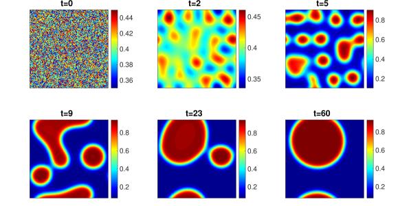
Figure 1: Time evolution of the polymer-solvent phase separation after a temperature quench with $\chi=3,\phi_{0}=0.4$ and $\omega=[-0.05,0.05]$. The computational domain is $\Omega=[0,1]\times[0,1]$ and the interface width $\sqrt{C_{0}}=\frac{1}{\sqrt{600}}$. The time step is $\Delta t=10^{-4}$.

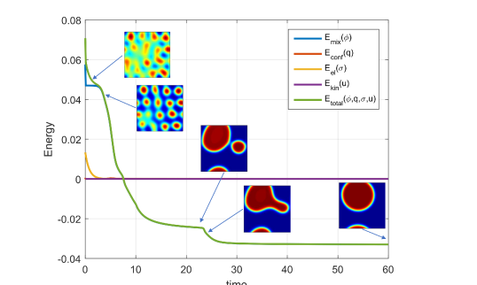
Figure 2: Energy evolution of the first numerical experiment corresponding to Figure 1 with intermediate states of the phase separation.

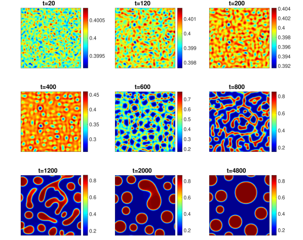
Figure 3: Time evolution of the polymer-solvent phase separation after a temperature quench with $\chi=2.\overline{54},\phi_{0}=0.4$ and $\omega=[-0.001,0.001]$. The computational domain is $\Omega=[0,128]\times[0,128]$ and the interface width $\sqrt{C_{0}}=1$. The time step is $\Delta t=0.025$.

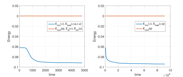
Figure 4: Energy evolution of the second numerical experiment corresponding to Figure 3 (left) and Figure 5 (right).

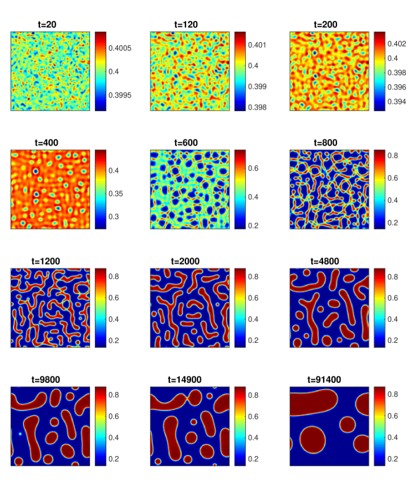
Figure 5: Time evolution of the polymer-solvent phase separation after a temperature quench, simulated by the simplified model utilizing the same parameter set used in the experiment from Figure 3, except for the time step $\Delta t=0.25$, since our second order scheme is used.

In the first numerical experiment we solve numerically system (7) applying periodic boundary conditions. The computational domain $\Omega=[0,1]\times[0,1]$ is divided into $128\times 128$ grid cells. We follow the parameter set from Gomez and Hughes [30]. The initial data of the volume fraction $\phi(t=0)$ is taken to be a constant $\phi_{0}=0.4$ with a random perturbation distributed in $\omega=[-0.05,0.05]$ and the initial velocities and bulk stress are set to zero. The initial value of the shear stress tensor is set to ${\boldsymbol{\sigma}}(t=0)=B_{2}(\phi(t=0))(\sqrt{2}-1)\mathbbm{1}$, which implies the positivity definiteness of the shear stress tensor. Further, we set the interface width $\sqrt{C_{0}}=\frac{1}{\sqrt{600}}$. For the Flory-Huggins potential the degrees of polymerization are set to $n_{p}=n_{s}=1$ and the temperature-dependent Flory interaction $\chi=3$. The bulk modulus is set to $A_{1}(\phi)=M^{0}_{b}\left[1+\tanh\left(\frac{\cot(\pi\phi^{*})-\cot(\pi\phi)}{\epsilon}\right)\right]+M^{1}_{b}$, where $M^{0}_{b}=0.5$ and $M^{1}_{b}=1$, $\phi^{*}$ is set to be equal to the initial average polymer volume fraction $\phi_{0}$ and $\epsilon=0.01$. Furthermore, we set the mobility coefficient $M=10$ and the relaxation coefficients to $\tau_{b}^{0}=10,\tau^{0}_{s}=5$ and $m^{0}_{s}=0.2$.

This experiment demonstrates phase separation by aggregation of the polymer molecules towards droplets. Figure 1 illustrates time evolution of the volume fraction $\phi$. The total energy is (strictly) monotonically decreasing over time, which is related to the surface minimization of the droplets and to droplets merging, see Figure 2.

The second experiment has been proposed in [7]. Here we solve numerically both, the complete system (7) as well as the simplified model (8). The computational domain $\Omega=[0,128]\times[0,128]$ is divided to $128\times 128$ grid cells, initial volume fraction consists of $\phi_{0}=0.4$ and a small random perturbation distributed in $\omega=[-0.001,0.001]$. The interface thickness width $\sqrt{C_{0}}=1$, which is already very small having the size of one grid cell, and the Flory interaction $\chi=2.\overline{54}$. The initial value of the shear stress is set to zero as in [7]. All other parameters are used as in the first experiment.

Figure 3 shows simulation of the complete system (7), where the whole viscoelastic phase separation process is exhibited. In the earlier stage the polymer-rich phase forms thin networklike structures. The solvent-rich droplets grow and coagulate. The area of the polymer-rich phase keeps decreasing. This is the well-known volume-shrinking process in polymer phase separation. In the later stage polymer-rich networklike structures are broken and the polymer-rich phase changes from being continuous to being discontinuous. This process is called phase inversion, cf. [7].

Figure 5 illustrate the dynamics of the simplified model (8). We can clearly see that also this model captures most important physical mechanism of the viscoelastic phase separation. From time $t=600$ thin networklike structures formed by the matrix-polymer-rich phase can be clearly recognized.

The presented experiments confirm the reliability of our newly developed methods that preserve thermodynamic consistency of the underlying physical model and dissipate free energy on the discrete level, see Figures 2 and 4. Consequently, they can be applied to model numerically complex polymeric mixtures and provide a detailed view in the dynamics of a phase separation process of a semi-dilute polymer-solvent mixture after a temperature quench, including both key characteristics volume-shrinking and phase inversion.

Conclusions

In this paper we have derived and analysed new linear, energy dissipative numerical schemes for viscoelastic phase separation. The mathematical model is obtained through the variational principle as a minimizer of the free energy. Consequently, the model consisting of the Cahn-Hilliard equation describing the dynamics of interface between polymer and Newtonian solvent and the Oldroyd-B for the viscoelastic flow, can be understood as the gradient flow corresponding to the total free energy.

The linearity of the numerical schemes increases the efficiency of numerical simulations since there is no nonlinear iterative process required. The energy dissipative property is fundamental for phase-separation problems and reflects their thermodynamic consistency on the discrete level. This property has been demonstrated experimentally and proven theoretically up to the numerical dissipation of the potential $ND_{phobic}$, which is small.

For the simplified model (8) the proposed numerical scheme is second order. Numerical experiments confirm that the simplified model can describe the most important physical properties of the viscoelastic phase separation. The full system can be approximated by the fully coupled scheme, Subsection 3.2 and the splitting scheme, Subsection 3.3. Both schemes yield analogous numerical solutions, but we opted here for the splitting scheme, since it is more efficient computationally.

In future our aim is to develop hybrid schemes for multiscale models of viscoelastic phase separation processes. Thus, our aim will be to combine the proposed linear, energy dissipative schemes for macroscopic models coupled with the combined Lattice-Boltzmann and Molecular-Dynamics simulations of mesoscopic models for the viscoelastic phase separation. We refer a reader to [31] and the references therein for more details on the latter scheme. We believe that by such hybrid multiscale simulation the underlying physics will become more clear and can provide deeper insight and perhaps also the development of more refined and accurate macroscopic models.

References

- [1] P. C. Hohenberg, B. I. Halperin, Theory of dynamic critical phenomena, Rev. Mod. Phys. 49 (3) (1977) 435–479. doi:10.1103/RevModPhys.49.435.
- [2] A. J. Bray, Theory of phase-ordering kinetics, Adv. Phys. 51 (2) (2002) 481–587. doi:10.1080/00018730110117433.
- [3] A. Onuki, Phase transition dynamics, Cambridge University Press, 2002.
- [4] H. Abels, D. Depner, H. Garcke, Existence of weak solutions for a diffuse interface model for two-phase flows of incompressible fluids with different densities, J. Math. Fluid Mech. 15 (3) (2013) 453–480. doi:10.1007/s00021-012-0118-x.
- [5] G. Tierra, F. Guillén-González, Numerical methods for solving the Cahn-Hilliard equation and its applicability to related energy-based models, Arch. Comput. Method. E. 22 (2) (2015) 269–289. doi:10.1007/s11831-014-9112-1.
- [6] F. Guillén-González, G. Tierra, On linear schemes for a Cahn-Hilliard diffuse interface model, J. Comput. Phys. 234 (2013) 140–171. doi:10.1016/j.jcp.2012.09.020.
- [7] D. Zhou, P. Zhang, W. E, Modified models of polymer phase separation, Phys. Rev. E 73 (6) (2006) 061801. doi:10.1103/PhysRevE.73.061801.
- [8] H. Tanaka, Viscoelastic phase separation, J. Phys. Condens. Mat. 12 (15) (2000) R207. doi:10.1088/0953-8984/12/15/201.
- [9] D. Kay, R. Welford, Efficient numerical solution of Cahn-Hilliard-Navier-Stokes fluids in 2d, SIAM J. Sci. Comput. 29 (6) (2007) 2241–2257. doi:10.1137/050648110.
- [10] Y. Cheng, A. Kurganov, Z. Qu, T. Tang, Fast and stable explicit operator splitting methods for phase-field models, J. Comput. Phys. 303 (2015) 45–65. doi:10.1016/j.jcp.2015.09.005.
- [11] D. Lee, J.-Y. Huh, D. Jeong, J. Shin, A. Yun, J. Kim, Physical, mathematical, and numerical derivations of the Cahn-Hilliard equation, Comp. Mater. Sci. 81 (2014) 216–225. doi:10.1016/j.commatsci.2013.08.027.
- [12] J. W. Barrett, S. Boyaval, Existence and approximation of a (regularized) Oldroyd-B model, Math. Mod. Meth. Appl. S. 21 (09) (2011) 1783–1837. doi:10.1142/S0218202511005581.
- [13] R. Fattal, R. Kupferman, Time-dependent simulation of viscoelastic flows at high Weissenberg number using the log-conformation representation, J. Non-Newton. Fluid 126 (1) (2005) 23–37. doi:10.1016/j.jnnfm.2004.12.003.
- [14] E. Fernández-Cara, F. M. Guillén-González, R. R. Ortega, Mathematical modeling and analysis of viscoelastic fluids of the Oldroyd kind, in: Handbook of numerical analysis (volume VIII), Elsevier, 2002, pp. 543–660.
- [15] M. Lukáčová-Medvid’ová, H. Notsu, B. She, Energy dissipative characteristic schemes for the diffusive Oldroyd-B viscoelastic fluid, Int. J. Numer. Meth. Fl. 81 (9) (2016) 523–557. doi:10.1002/fld.4195.
- [16] M. Lukáčová-Medvid’ová, B. Dünweg, P. Strasser, N. Tretyakov, Energy-stable numerical schemes for multiscale simulations of polymer-solvent mixtures, in: P. van Meurs, M. Kimura, H. Notsu (Eds.), Mathematical Analysis of Continuum Mechanics and Industrial Applications II, Vol. 30 of Mathematics for Industry, Springer Singapore, 2018, pp. 153–165. doi:10.1007/978-981-10-6283-4.
- [17] J. W. Cahn, J. E. Hilliard, Free energy of a nonuniform system. I. Interfacial free energy, J. Chem. Phys. 28 (1958) 258–267. doi:10.1063/1.1744102.
- [18] C. M. Elliott, S. Zheng, On the Cahn-Hilliard equation, Arch. Rat. Mech. Anal. 96 (1986) 339–357.
- [19] C. M. Elliott, H. Garcke, On the Cahn-Hilliard equation with degenerate mobility, SIAM J. Math. Anal. 27 (1996) 404–423.
- [20] C. M. Elliott, H. Garcke, Diffusional phase transitions in multicomponent systems with a concentration dependent mobility matrix, Physica D 109 (1997) 242–256.
- [21] P. J. Flory, Thermodynamics of high polymer solutions, J. Chem. Phys 10 (1942) 51–61.
- [22] M. L. Huggins, Thermodynamics of high polymer solutions, J. Chem. Phys 9 (1941) 440.
- [23] X. Wu, G. J. van Zwieten, K. G. van der Zee, Stabilized second-order convex splitting schemes for Cahn-Hilliard models with application to diffuse-interface tumor-growth models, Int. J. Numer. Meth. Bio. 30 (2) (2014) 180–203. doi:10.1002/cnm.2597.
- [24] F. Guillén-González, M. Á. Rodríguez-Bellido, G. Tierra, Linear unconditional energy-stable splitting schemes for a phase-field model for nematic-isotropic flows with anchoring effects, Int. J. Numer. Meth. Eng. 108 (6) (2016) 535–567. doi:10.1002/nme.5221.
- [25] H. Tanaka, T. Araki, Phase inversion during viscoelastic phase separation: Roles of bulk and shear relaxation moduli, Phys. Rev. Lett. 78 (1997) 4966–4969. doi:10.1103/PhysRevLett.78.4966.
- [26] D. Hu, T. Lelièvre, New entropy estimates for the Oldroyd-B model and related models, Commun. Math. Sci. 5 (4) (2007) 909–916.
- [27] X. Yang, J. Zhao, On linear and unconditionally energy stable algorithms for variable mobility Cahn-Hilliard type equation with logarithmic Flory-Huggins potential, arXiv:1701.07410 [math.NA].
- [28] A. J. Chorin, A numerical method for solving incompressible viscous flow problems, J. Comput. Phys. 2 (1967) 12–26. doi:10.1016/0021-9991(67)90037-X.
- [29] F. H. Harlow, J. E. Welch, Numerical calculation of time-dependent viscous incompressible flow of fluid with free surface, Phys. Fluids 8 (12) (1965) 2182–2189. doi:10.1063/1.1761178.
- [30] H. Gómez, T. J. R. Hughes, Provably unconditionally stable, second-order time-accurate, mixed variational methods for phase-field models, J. Comput. Phys. 230 (2011) 5310–5327.
- [31] N. Tretyakov, B. Dünweg, An improved dissipative coupling scheme for a system of Molecular Dynamics particles interacting with a Lattice Boltzmann fluid, Computer Phys. Comm. 216 (2017) 102–108.