A Riesz basis Galerkin method for the tempered fractional Laplacian

Abstract

The fractional Laplacian $\Delta^{\beta/2}$ is the generator of $\beta$-stable Lévy process, which is the scaling limit of the Lévy fight. Due to the divergence of the second moment of the jump length of the Lévy fight it is not appropriate as a physical model in many practical applications. However, using a parameter $\lambda$ to exponentially temper the isotropic power law measure of the jump length leads to the tempered Lévy fight, which has finite second moment. For short time the tempered Lévy fight exhibits the dynamics of Lévy fight while after sufficiently long time it turns to normal diffusion. The generator of tempered $\beta$-stable Lévy process is the tempered fractional Laplacian $(\Delta+\lambda)^{\beta/2}$ [W.H. Deng, B.Y. Li, W.Y. Tian, and P.W. Zhang, Multiscale Model. Simul., in press, 2017]. In the current work, we present new computational methods for the tempered fractional Laplacian equation, including the cases with the homogeneous and nonhomogeneous generalized Dirichlet type boundary conditions. We prove the well-posedness of the Galerkin weak formulation and provide convergence analysis of the single scaling B-spline and multiscale Riesz bases finite element methods. We propose a technique for efficiently generating the entries of the dense stiffness matrix and for solving the resulting algebraic equation by preconditioning. We also present several numerical experiments to verify the theoretical results.

1 Introduction

Phenomena of anomalous diffusion are ubiquitous in nature [25]. Lévy flights with isotropic power law measure $|x|^{-n-\beta}$ of the jump length display superdiffusion, where $n$ is the dimension of space and $\beta\in(0,2)$ is a parameter. The scaling limit of Lévy flight is the $\beta$-stable Lévy process, the generator of which is the fractional Laplacian $\Delta^{\beta/2}$. This topic has recently become popular in both pure and applied mathematical communities [26]. The divergence of second moment of the Lévy flight is associated with the possible infinite speed of the motion of the particles, which contradicts their nonzero masses, i.e., the pure power law distribution of jump length sometimes makes the Lévy flight not a suitable physical model. Hence, tempering the distribution of the jump length becomes a natural idea, namely, modify $|x|^{-n-\beta}$ as $e^{-\lambda|x|}|x|^{-n-\beta}$ with $\lambda$ being a small nonnegative real number, so that we can obtain the tempered Lévy flight.

For small $\lambda$, the tempered Lévy flight exhibits a slow transition of the dynamics from Lévy flight to normal diffusion, which may occur after sufficient long time. The scaling limit of the tempered Lévy flight is called tempered Lévy process, the generator of which is the tempered fractional Laplacian $(\Delta+\lambda)^{\beta/2}$ [9]. In this paper, we mainly focus on developing numerical methods in the Riesz basis Galerkin framework for the tempered fractional Laplacian, i.e.

(3) $$\left\{\begin{array}[]{ll}-(\Delta+\lambda)^{\beta/2}p(x)=f(x),&~{}~{}x\in\Omega,\\ p(x)=0,&~{}~{}x\in\mathbb{R}\backslash\Omega,\end{array}\right.$$

which corresponds to the one-dimensional case of the initial and boundary value problem in Eq. (49) recently proposed in [9]. Here $\beta\in(0,2),\,\lambda\geq 0,\,\Omega=(a,b),\,f(x)\in H^{-\beta/2}(\Omega)$, and

(4) $$(\Delta+\lambda)^{\beta/2}p(x):=-c_{\beta}{~{}\rm P.V.~{}}\int_{\mathbb{R}}\frac{p(x)-p(y)}{e^{\lambda|x-y|}|x-y|^{1+\beta}}dy$$

with

(7) $$c_{\beta}=\left\{\begin{array}[]{ll}\frac{\beta\Gamma(\frac{1+\beta}{2})}{2^{1-\beta}\pi^{1/2}\Gamma(1-\beta/2)}&~{}{\rm for~{}}\lambda=0~{}{\rm or}~{}\beta=1,\\[3.0pt] \frac{\Gamma(\frac{1}{2})}{2\pi^{\frac{1}{2}}|\Gamma(-\beta)|}&~{}{\rm for}~{}\lambda>0~{}{\rm and}~{}\beta\not=1,\end{array}\right.$$

where P.V. denotes the Cauchy principle value, being the limit of the integral over $\mathbb{R}\backslash B_{\epsilon}(x)$ as $\epsilon\to 0$; the definition of this form is indeed necessary when $\beta\geq 1$.

Obviously, when $\lambda=0$, (4) reduces to fractional Laplacian

(8) $$\Delta^{\beta/2}p(x):=-c_{\beta}{~{}\rm P.V.~{}}\int_{\mathbb{R}}\frac{p(x)-p(y)}{|x-y|^{1+\beta}}dy,$$

which has the Fourier transform (assuming that $\mathscr{F}[\Delta^{\beta/2}p(x)](\xi)$ and $\mathscr{F}[p(x)](\xi)$ exist)

(9) $$\mathscr{F}[\Delta^{\beta/2}p(x)](\xi)=-|\xi|^{\beta}\mathscr{F}[p(x)](\xi).$$

Here $\mathscr{F}[w(x)](\xi),\,\xi\in\mathbb{R}$ is defined by $\mathscr{F}[w(x)](\xi)=\int_{\mathbb{R}}w(x)e^{-ix\xi}dx$, and for $w_{1},w_{2}\in L^{2}(\mathbb{R})$, the Parseval identity [17, pp. 100] can be applied

(10) $$\int_{\mathbb{R}}w_{1}(x)\overline{w_{2}(x)}dx=\frac{1}{2\pi}\int_{\mathbb{R}}\mathscr{F}[w_{1}(x)](\xi)\overline{\mathscr{F}[w_{2}(x)](\xi)}d\xi.$$

Recently, the fractional Laplacian has attracted a lot of attention, but even in the simplified context [1, 2, 11, 19] it is far from the well-developed status of the classical Laplacian. The numerical resolution of the fractional Laplacian involves two major challenging tasks, namely the singular kernel and the integration in an unbounded region. For the finite difference method the convergence rate is even influenced by the regularity of the exact solution outside of the domain $\Omega$ [19]. As for the tempered fractional differential equations, there are some published works on numerical methods [4, 18, 22, 33], but no theoretical results under the variational framework exists. In the current paper we prove the well-posedness of the variational formulation of (3), where extra efforts must be made to obtain the $\tilde{H}^{\beta/2}(\mathbb{R})$-coercivity. Subsequently, the convergence analysis and the effective implementation of the finite dimensional approximation with the single-scale or multiscale basis functions are presented, in which the properties of Riesz basis and multiresolution are used.

The rest of this paper is organized as follows. In Section 2, we introduce the function spaces and the properties of the tempered fractional Laplacian to be used. The variational formulation of (3) and its well-posedness are presented and discussed in Section 3. We develop the Riesz basis Galerkin approximation and perform its convergence analysis in Section 4. Section 5 provides the effective implementations, including calculating the entries of the stiffness matrix and solving the resulting algebraic equations. We discuss the model (3) with nonhomogeneous generalized Dirichlet type boundary condition in Section 6. The numerical results are given in Section 7 and we conclude the paper with remarks in Section 8.

2 Preliminaries

Throughout the paper by the notation $A\lesssim B$ we mean that $A$ can be bounded by a multiple of $B$, independent of the parameters they may depend on, while the expression $A\simeq B$ means that $A\lesssim B\lesssim A$. Let $E$ be an open set of $\mathbb{R}$. If $s\geq 0$ is a nonnegative integer, we denote by $H^{s}(E)$ the classical Sobolev space equipped with the norm

(11) $$\|w\|_{H^{s}(E)}:=\left(\sum_{0\leq k\leq s}\left\|w^{(k)}\right\|^{2}_{L^{2}(E)}\right)^{1/2},$$

where $w^{(k)}$ stands for the $k$-th distributional derivative, and $H^{0}(E):=L^{2}(E)$. In the following, we define the fractional Sobolev spaces, where $s$ is not an integer.

For a fixed $s\in(0,1)$, the Sobolev space $H^{s}(E)$ is defined as

(12) $$H^{s}(E):=\left\{w\in L^{2}(E):|w|_{H^{s}(E)}<\infty\right\},$$

where

(13) $$|w|_{H^{s}(E)}:=\left(\int_{E}\int_{E}\frac{\left|w(x)-w(y)\right|^{2}}{|x-y|^{1+2s}}dxdy\right)^{1/2}$$

is the Slobodeckii semi-norm [24, pp. 74] of $w(x)$ . The space $H^{s}(E)$ is a Banach space, endowed with the natural norm

(14) $$\left\|w\right\|_{H^{s}(E)}:=\left(\left\|w\right\|_{L^{2}(E)}^{2}+|w|^{2}_{H^{s}(E)}\right)^{1/2}.$$

Indeed, $H^{s}(E)$ also is a Hilbert space [24, pp. 75]. For $s>1$ and $s\notin\mathbb{N}$, we can define $H^{s}(E)$ as follows:

(15) $$H^{s}(E):=\left\{w\in H^{\lfloor s\rfloor}(E):\left|w^{(\lfloor s\rfloor)}\right|_{H^{s-\lfloor s\rfloor}(E)}<\infty\right\},$$

where $\lfloor s\rfloor$ is the biggest integer smaller than $s$. In this case, $H^{s}(E)$ is endowed with the norm

(16) $$\left\|w\right\|_{H^{s}(E)}:=\left(\left\|w\right\|^{2}_{H^{\lfloor s\rfloor}(E)}+\left|w^{(\lfloor s\rfloor)}\right|^{2}_{H^{s-\lfloor s\rfloor}(E)}\right)^{1/2}.$$

We note that $H^{s}(E)$ is a well-defined Banach space for every $s\geq 0$. Moreover, when $E=\mathbb{R}$, for $0<s<1$, it holds that $\left|w\right|^{2}_{H^{s}(\mathbb{R})}\simeq\int_{\mathbb{R}}|\xi|^{2s}|\mathscr{F}[w](\xi)|^{2}d\xi$, and for $s>0$, $\left\|w\right\|^{2}_{H^{s}(\mathbb{R})}\simeq\int_{\mathbb{R}}\left(1+|\xi|^{2s}\right)|\mathscr{F}[w](\xi)|^{2}d\xi$ [24, pp. 79-80]. In fact, the Sobolev space $H^{s}(\mathbb{R})$ can also be defined as

(17) $$H^{s}(\mathbb{R})=\left\{w\in L^{2}(\mathbb{R}):\int_{\mathbb{R}}\left(1+|\xi|^{2s}\right)|\hat{w}(\xi)|^{2}d\xi<\infty\right\}.$$

Let $C_{0}^{\infty}(E)$ be the space of functions that are infinite differentiable on $E$ and have compact support in $E$. Then $C_{0}^{\infty}(\mathbb{R})$ is dense in $H^{s}(\mathbb{R})$. However, if $E\subset\mathbb{R}$ is strict, the space $C_{0}^{\infty}(E)$ generally is not dense in $H^{s}(E)$. Hence, we denote by $H_{0}^{s}(E)$ the closure of $C_{0}^{\infty}(E)$ in $H^{s}(E)$. As usual, $H^{-s}(E)$ is the dual space of $H_{0}^{s}(E)$. In addition, let $\Omega=(a,b)$ be a nonempty open interval of $\mathbb{R}$. By $\tilde{C}_{0}^{\infty}(\Omega)$ we denote the space of all infinitely differentiable functions on $\mathbb{R}$ whose support is compact and contained in $\Omega$. For $s>0$, we use $\tilde{H}_{0}^{s}(\Omega)$ to denote the closure of $\widetilde{C}_{0}^{\infty}(\Omega)$ in $H^{s}(\mathbb{R})$. For $s=0$, $\widetilde{H}_{0}^{s}(\Omega)$ is interpreted as the closure of $\widetilde{C}_{0}^{\infty}(\Omega)$ in $L^{2}(\mathbb{R})$, and denoted as $\widetilde{L}^{2}(\Omega)$. Obviously, $\widetilde{H}_{0}^{s}(\Omega)\subset H_{0}^{s}(\Omega)$. Moreover, by [15], when $s\in(0,1)$, $\widetilde{H}^{s}_{0}(\Omega)$ can also be defined by

(18) $$\widetilde{H}_{0}^{s}(\Omega)=\left\{w(x)\in H^{s}(\mathbb{R}):w(x)=0~{}{\rm a.e.~{}for~{}}x\in\mathbb{R}\backslash\Omega\right\}.$$

Here, the space $\widetilde{C}_{0}^{\infty}(\Omega)$ is actually the space $C_{c}^{\infty}(a,b)$ in [20, pp. 178] and the space $C_{0}^{\infty}(a,b)$ in [15, pp. 237]. The space $\widetilde{H}_{0}^{s}(\Omega)$ is the space $H_{0}^{\mu}(a,b)$ with $\mu=s$ in [20, pp. 178] and the space $X_{0}^{s,p}(a,b)$ with $p=2$ in [15, pp. 236–237].

Next, we give some properties of the tempered fractional Laplacian.

Proposition 1.

For $w(x)\in C_{0}^{\infty}(\mathbb{R})$ and $\lambda>0$, we have

(19) $$\mathscr{F}\left[(\Delta+\lambda\right)^{\beta/2}w(x)](\xi)$$

$$~{}=(-1)^{\lfloor\beta\rfloor}\left(\lambda^{\beta}-\left(\lambda^{2}+\left|\xi\right|^{2}\right)^{\frac{\beta}{2}}\cos\left(\beta\arctan\left(\frac{\left|\xi\right|}{\lambda}\right)\right)\right)\mathscr{F}[w](\xi)$$

for $\beta\in(0,1)\cup(1,2)$, and

$$\mathscr{F}\left[(\Delta+\lambda\right)^{\beta/2}w(x)](\xi)$$

(20) $$~{}~{}=\frac{2}{\pi}\left(-\left|\xi\right|\arctan\left(\frac{\left|\xi\right|}{\lambda}\right)+\frac{\lambda}{2}\ln(\lambda^{2}+\left|\xi\right|^{2})-\lambda\ln(\lambda)\right)\mathscr{F}[w](\xi)$$

for $\beta=1$, where $\lfloor\beta\rfloor:=\left\{z\in\mathbb{N}:0\leq\beta-z<1\right\}$.

Proof.

For $w\in C_{0}^{\infty}(\mathbb{R})$, it holds that

(21) $$\left(\Delta+\lambda\right)^{\beta/2}w(x)=\frac{-c_{\beta}}{2}\int_{\mathbb{R}}\frac{2w(x)-w(x-y)-w(x+y)}{e^{\lambda|y|}|y|^{1+\beta}}dy.$$

So $\left(\Delta+\lambda\right)^{\beta/2}w(x)$ make sense for $x\in\mathbb{R}$. Then

$$\mathscr{F}\left[(\Delta+\lambda\right)^{\beta/2}w(x)](\xi)=-c_{\beta}\int_{0}^{\infty}\frac{2-e^{-iy\xi}-e^{iy\xi}}{e^{\lambda y}y^{1+\beta}}dy\,\mathscr{F}[w](\xi)$$

$$~{}~{}=-c_{\beta}\int_{0}^{\infty}\left(2-2\cos(y\xi)\right)e^{-\lambda y}y^{-1-\beta}dy\,\mathscr{F}[w](\xi)$$

$$~{}~{}=\frac{c_{\beta}}{\beta}\int_{0}^{\infty}\left(2-2\cos(y\xi)\right)e^{-\lambda y}d\left(y^{-\beta}\right)\,\mathscr{F}[w](\xi)$$

(22) $$~{}~{}=\frac{2c_{\beta}}{-\beta}\int_{0}^{\infty}y^{-\beta}e^{-\lambda y}\left(\xi\sin(y\xi)-\lambda(1-\cos(y\xi))\right)dy\,\mathscr{F}[w](\xi).$$

Since $\xi\sin(y\xi)-\lambda(1-\cos(y\xi)$ is an even function w.r.t. $\xi$, in the following we assume $\xi\geq 0$.

If $0<\beta<1$, we have

$$\int_{0}^{\infty}y^{-\beta}e^{-\lambda y}\left(\xi\sin(y\xi)-\lambda(1-\cos(y\xi))\right)dy$$

$$~{}=\xi\int_{0}^{\infty}y^{-\beta}e^{-\lambda y}\sin(y\xi)dy-\lambda\int_{0}^{\infty}y^{-\beta}e^{-\lambda y}dy+\lambda\int_{0}^{\infty}y^{-\beta}e^{-\lambda y}\cos(y\xi)dy$$

$$~{}=\frac{\Gamma(1-\beta)\xi}{\left(\lambda^{2}+\xi^{2}\right)^{\frac{1-\beta}{2}}}\sin\left((1-\beta)\arctan\left(\frac{\xi}{\lambda}\right)\right)-\lambda^{\beta}\int_{0}^{\infty}y^{-\beta}e^{-y}dy$$

$$~{}~{}~{}+\frac{\Gamma(1-\beta)\lambda}{\left(\lambda^{2}+\xi^{2}\right)^{\frac{1-\beta}{2}}}\cos\left((1-\beta)\arctan\left(\frac{\xi}{\lambda}\right)\right)$$

(23) $$~{}={\Gamma(1-\beta)}{\left(\lambda^{2}+\xi^{2}\right)^{\frac{\beta}{2}}}\cos\left(\beta\arctan\left(\frac{\left|\xi\right|}{\lambda}\right)\right)-\lambda^{\beta}\Gamma(1-\beta),$$

where the formulae [16, Eq. (3.944(5))] and [16, Eq. (3.944(6))] have been used in the second step.

For $1<\beta<2$, using the integration by parts again, and similarly we have

$$\int_{0}^{\infty}y^{-\beta}e^{-\lambda y}\left(\xi\sin(y\xi)-\lambda(1-\cos(y\xi))\right)dy$$

$$~{}=\frac{1}{1-\beta}\int_{0}^{\infty}e^{-\lambda y}y^{1-\beta}\left(\left(\lambda^{2}-\xi^{2}\right)\cos(y\xi)+2\lambda\xi\sin(y\xi)-\lambda^{2}\right)dy$$

$$~{}=\frac{\Gamma(1-\beta)}{(\lambda^{2}+\xi)^{1-\frac{\beta}{2}}}\bigg{(}\left(\lambda^{2}-\xi^{2}\right)\cos\left(\left(2-\beta\right)\arctan\left(\frac{\xi}{\lambda}\right)\right)$$

$$~{}~{}~{}+2\lambda\xi\sin\left(\left(2-\beta\right)\arctan\left(\frac{\xi}{\lambda}\right)\right)\bigg{)}-\Gamma(1-\beta)\lambda^{\beta}$$

(24) $$~{}={\Gamma(1-\beta)}{\left(\lambda^{2}+\xi^{2}\right)^{\frac{\beta}{2}}}\cos\left(\beta\arctan\left(\frac{\left|\xi\right|}{\lambda}\right)\right)-\lambda^{\beta}\Gamma(1-\beta).$$

For $\beta=1$, using the integration by parts, we have

$$\int_{0}^{\infty}y^{-\beta}e^{-\lambda y}\left(\xi\sin(y\xi)-\lambda(1-\cos(y\xi))\right)dy$$

$$~{}=\left(\lambda^{2}-\xi^{2}\right)\int_{0}^{\infty}\ln(y)e^{-\lambda y}\left(\cos(y\xi)\right)dy$$

$$~{}~{}~{}+2\lambda\xi\int_{0}^{\infty}\ln(y)e^{-\lambda y}\sin(u\xi)dy-\lambda^{2}\int_{0}^{\infty}\ln(y)e^{-\lambda y}dy$$

$$~{}=\frac{2\lambda\xi}{\lambda^{2}+\xi^{2}}\left(\lambda\arctan\left(\frac{\xi}{\lambda}\right)-\gamma\xi-\frac{\xi}{2}\ln(\lambda^{2}+\xi^{2})\right)$$

$$~{}~{}~{}+\frac{\xi^{2}-\lambda^{2}}{\lambda^{2}+\xi^{2}}\left(\frac{\lambda}{2}\ln\left(\lambda^{2}+\xi^{2}\right)+\xi\arctan\left(\frac{\xi}{\lambda}\right)+\lambda\gamma\right)+\lambda\left(\gamma+\ln(\lambda)\right)$$

(25) $$~{}=\xi\arctan\left(\frac{\xi}{\lambda}\right)-\frac{\lambda}{2}\ln(\lambda^{2}+\xi^{2})+\lambda\ln(\lambda),$$

where $\gamma$ denotes the Euler constant, and the formulae [16, Eq. (4.441(1))-(4.441(2))] and [16, Eq. (4.331(1))] have been used in the second step. ∎

The following proposition is similar to Theorem 2.1 of [21].

Proposition 2.

For $0<\beta<2$, the tempered fractional Laplacian can be extended to a continuous linear mapping from $H^{\beta}(\mathbb{R})$ to $L^{2}(\mathbb{R})$, and its Fourier transform remains the same.

Proof.

Firstly, assume $w\in C_{0}^{\infty}(\mathbb{R})$. For $\lambda=0$, by

(26) $$\mathscr{F}[\Delta^{\beta/2}w(x)](\xi)=-\left|\xi\right|^{\beta}\mathscr{F}\left[w(x)\right](\xi),$$

and the Parseval identity (10), we have

(27) $$\left\|\Delta^{\beta/2}w\right\|^{2}_{L^{2}(\mathbb{R})}=\frac{1}{2\pi}\int_{\mathbb{R}}\left|\xi\right|^{2\beta}\left|\mathscr{F}\left[w(x)\right](\xi)\right|^{2}d\xi\leq\left\|w\right\|^{2}_{H^{\beta}(\mathbb{R})}.$$

For $\lambda>0$, by Proposition 1 and the Parseval identity (10), we have

$$\left\|\left(\Delta+\lambda\right)^{\beta/2}w\right\|^{2}_{L^{2}(\mathbb{R})}\leq\int_{\mathbb{R}}\mathcal{G}^{2}(\lambda,\xi,\beta)\left|\mathscr{F}[w(x)](\xi)\right|^{2}d\xi$$

(28) $$~{}\lesssim\int_{\mathbb{R}}\left(1+|\xi|^{2\beta}\right)\left|\mathscr{F}[w(x)](\xi)\right|^{2}d\xi\lesssim\left\|w\right\|^{2}_{H^{\beta}(\mathbb{R})},$$

where

(31) $$~{}~{}~{}~{}\mathcal{G}(\lambda,\xi,\beta):=\left\{\begin{array}[]{l}(-1)^{\lfloor\beta\rfloor}\left(\left(\lambda^{2}+\left|\xi\right|^{2}\right)^{\frac{\beta}{2}}\cos\left(\beta\arctan(\frac{\left|\xi\right|}{\lambda})\right)-\lambda^{\beta}\right),~{}\beta\not=1,\\ \frac{2}{\pi}\left(\left|\xi\right|\arctan\left(\frac{\left|\xi\right|}{\lambda}\right)-\frac{\lambda}{2}\ln(\lambda^{2}+\left|\xi\right|^{2})+\lambda\ln(\lambda)\right),~{}~{}~{}\beta=1;\end{array}\right.$$

and the inequalities $\left(x_{1}+x_{2}+x_{3}\right)^{2}\leq 3\left(x_{1}^{2}+x_{2}^{2}+x_{3}^{2}\right),\,\cos\left(\beta\arctan\left(\frac{\left|\xi\right|}{\lambda}\right)\right)\leq 1$, $\arctan\left(\frac{\left|\xi\right|}{\lambda}\right)\leq\frac{\pi}{2},\,\ln(\lambda^{2}+|\xi|^{2})\leq\lambda^{2}+|\xi|^{2}$, and $\left(\lambda^{2}+|\xi|^{2}\right)^{\beta}\leq 2^{\beta}\left(\lambda^{2\beta}+|\xi|^{2\beta}\right)$, have been used. Then by the density of $C_{0}^{\infty}(\mathbb{R})$ in $H^{\beta}(\mathbb{R})$, one can continuously extend $\left(\Delta+\lambda\right)^{\beta/2}$ to an operator from $H^{\beta}(\mathbb{R})$ to $L^{2}(\mathbb{R})$.

Secondly, let $w\in H^{\beta}(\mathbb{R})$. Then $\mathscr{F}[\left(\Delta+\lambda\right)^{\beta/2}w(x)](\xi)\in L^{2}(\mathbb{R})$, and there exists a sequence $\left\{w_{k}\right\}\in C_{0}^{\infty}(\mathbb{R})$ such that $\lim_{k\to\infty}\left\|w-w_{k}\right\|_{H^{\beta}(\mathbb{R})}=0$. Therefore, for $\lambda>0$, by (28) and the Parseval identity we have

$$\left\|-\mathcal{G}(\lambda,\xi,\beta)\mathscr{F}[w(x)](\xi)-\mathscr{F}[\left(\Delta+\lambda\right)^{\beta/2}w(x)](\xi)\right\|_{L^{2}(\mathbb{R})}$$

$$~{}\leq\left\|-\mathcal{G}(\lambda,\xi,\beta)\mathscr{F}\left[w(x)-w_{k}\right](\xi)\right\|_{L^{2}(\mathbb{R})}$$

$$~{}~{}~{}+\left\|\mathscr{F}\left[\left(\Delta+\lambda\right)^{\beta/2}(w_{k}-w)(x)\right](\xi)\right\|_{L^{2}(\mathbb{R})}$$

(32) $$~{}\leq 2\left\|w-w_{k}\right\|_{H^{\beta}(\mathbb{R})}\to 0.$$

Thus $\mathscr{F}\left[\left(\Delta+\lambda\right)^{\beta/2}w(x)\right](\xi)=-\mathcal{G}(\lambda,\xi,\beta)\mathscr{F}[w(x)](\xi)$. The proof for $\lambda=0$ is similar. ∎

Proposition 3.

If $w(x)\in C^{3}(\mathbb{R})$ and $w(x),\,w^{(3)}(x)\in L^{\infty}(\mathbb{R})$, for $\lambda\geq 0$, we have

(33) $$\lim_{\beta\to 2^{-}}(\Delta+\lambda)^{\beta/2}w(x)=\frac{d^{2}w(x)}{dx^{2}}.$$

Proof.

For $\lambda>0$, following the definition of tempered fractional Laplacian, we have

$$\left|{c_{\beta}}\int_{0}^{\infty}\frac{w(x+y)-2w(x)+w(x-y)-w^{(2)}(x)y^{2}}{e^{\lambda y}y^{1+\beta}}dy\right|$$

$$~{}\leq c_{\beta}\big{\|}w^{(3)}\big{\|}_{L^{\infty}(\mathbb{R})}\int_{0}^{\infty}\frac{y^{3}}{y^{1+\beta}e^{\lambda y}}dy$$

$$~{}=c_{\beta}\lambda^{\beta-3}\Gamma(3-\beta)\big{\|}w^{(3)}\big{\|}_{L^{\infty}(\mathbb{R})}\to 0,~{}~{}~{}\beta\to 2^{-},$$

where $c_{\beta}=\frac{\Gamma(\frac{1}{2})}{2\pi^{\frac{1}{2}}|\Gamma(-\beta)|}$. Further note that

$${c_{\beta}}\int_{0}^{\infty}\frac{w^{(2)}(x)y^{2}}{e^{\lambda y}y^{1+\beta}}dy=w^{(2)}(x)c_{\beta}\lambda^{\beta-2}\Gamma(2-\beta)$$

$$~{}=w^{(2)}(x)\frac{(1-\beta)(-\beta)}{2}\to w^{(2)}(x),~{}~{}\beta\to 2^{-},$$

which results in the desired result.

For the case $\lambda=0$, note that

$$\left|{c_{\beta}}\int_{c}^{\infty}\frac{w(x+y)-2w(x)+w(x-y)}{y^{1+\beta}}dy\right|$$

$$~{}=4c_{\beta}\left\|w\right\|_{L^{\infty}(\mathbb{R})}\int_{c}^{\infty}\frac{1}{y^{1+2s}}dy\to 0,~{}~{}~{}\beta\to 2^{-};$$

$$\left|{c_{\beta}}\int_{0}^{c}\frac{w(x+y)-2w(x)+w(x-y)-w^{(2)}(x)y^{2}}{e^{\lambda y}y^{1+\beta}}dy\right|$$

$$~{}=c_{\beta}\frac{c^{3-\beta}}{3-\beta}\big{\|}w^{(3)}\big{\|}_{L^{\infty}(\mathbb{R})}\to 0,~{}~{}~{}\beta\to 2^{-},$$

where $c\geq 0$ is an arbitrary given constant, and $c_{\beta}=\frac{\beta\Gamma(\frac{1+\beta}{2})}{2^{1-\beta}\pi^{1/2}\Gamma(1-\beta/2)}$. Therefore,

$$\left(\Delta+\lambda\right)^{\beta/2}w(x)={c_{\beta}}\int_{0}^{d}\frac{w^{(2)}(x)y^{2}}{y^{1+\beta}}dy=\frac{c_{\beta}}{2-\beta}d^{2-\beta}w^{(2)}(x).$$

By [26, pp. 25]

$$c_{\beta}=\frac{1}{\pi}\Gamma(1+\beta)\sin\left(\frac{\beta\pi}{2}\right)=\frac{1}{\pi}\Gamma(1+\beta)\sin\left(\frac{(2-\beta)\pi}{2}\right),$$

we have $\lim_{\beta\to 2^{-}}\frac{c_{\beta}}{2-\beta}d^{2-\beta}w^{(2)}(x)=w^{(2)}(x)$. ∎

Equation (33) shows that if $\beta\to 2^{-}$, the tempered fractional Laplacian coincides with the classical Laplacian. Finally, we give the concept of Riesz basis that will be used later.

Definition 4 ([20, 30]).

A countable collection of elements $\mathcal{E}:=\left\{e_{i}\right\}_{i\in I}\,(I\subset\mathbb{Z})$ of a Hilbert space $H$ is called a Riesz basis of $H$ if each element in $H$ has an expansion in terms of $\mathcal{E}$ and there exists (Riesz) constants $0<A\leq B<\infty$ such that

(34) $$A\sum_{i\in I}|d_{i}|^{2}\leq\bigg{\|}\sum_{i\in I}d_{i}e_{i}\bigg{\|}_{H}^{2}\leq B\sum_{i\in I}|d_{i}|^{2}.$$

3 Weak solution and well-posedness

In this section, we first give the definition of the weak solution of (3), and then discuss the well-posedness of the corresponding weak formulation. As in the usual approach in dealing with elliptic PDE, multiplying both sides of (3) by $v\in\widetilde{C}^{\infty}_{0}(\Omega)$ and integrating them over $\Omega$ leads to

(35) $$c_{\beta}\int_{\mathbb{R}}\int_{\mathbb{R}}\frac{\left(p(x)-p(y)\right)v(x)}{e^{\lambda|x-y|}\left|x-y\right|^{1+\beta}}dydx=\int_{\Omega}f(x)v(x)dx.$$

Instead of performing integration by parts, we use the fact

(36) $$\int_{\mathbb{R}}\int_{\mathbb{R}}\frac{\left(p(x)-p(y)\right)v(x)}{e^{\lambda|x-y|}\left|x-y\right|^{1+\beta}}dydx=\int_{\mathbb{R}}\int_{\mathbb{R}}\frac{\left(p(y)-p(x)\right)v(y)}{e^{\lambda|y-x|}\left|y-x\right|^{1+\beta}}dydx$$

to get the weak formulation of (3): find $p\in{\widetilde{H}_{0}^{\beta/2}(\Omega)}$ such that

(37) $$B(p,v)=\langle f,v\rangle$$

for all $v\in{\widetilde{H}_{0}^{\beta/2}(\Omega)}$, where the duality pairing $\left\langle f,v\right\rangle:=\int_{\Omega}f(x)v(x)dx$ and the bilinear form

(38) $$B(p,v):=\frac{c_{\beta}}{2}\int_{\mathbb{R}}\int_{\mathbb{R}}\frac{\left(p(x)-p(y)\right)\left(v(x)-v(y)\right)}{e^{\lambda|x-y|}\left|x-y\right|^{1+\beta}}dydx.$$

When $\lambda=0$, Ref. [9] gives the weak formulation of (3) as: find $p\in{\widetilde{H}_{0}^{\beta/2}(\Omega)}$, such that

(39) $$\int_{\mathbb{R}}\Delta^{\beta/4}p\,\Delta^{\beta/4}vdx=\int_{\Omega}fvdx~{}~{}~{}~{}\forall v\in{\widetilde{H}_{0}^{\beta/2}(\Omega)},$$

being equivalent to (37) with $\lambda=0$. In fact, it can be simply verified as: for any $p,v\in\widetilde{H}_{0}^{\beta/2}(\Omega)$, by the Parseval identity (10) and $\mathscr{F}[\Delta^{\beta/4}p(x)](\xi)=-|\xi|^{\beta/2}\mathscr{F}[p(x)](\xi)$,

$$\frac{c_{\beta}}{2}\int_{\mathbb{R}}\int_{\mathbb{R}}\frac{\left(p(x)-p(y)\right)\left(v(x)-v(y)\right)}{\left|x-y\right|^{1+\beta}}dydx$$

$$~{}~{}=\frac{c_{\beta}}{2}\int_{\mathbb{R}}\int_{\mathbb{R}}\frac{(p(x+y)-p(y))(v(x+y)-v(y))}{|x|^{1+\beta}}dydx$$

$$~{}~{}=\frac{c_{\beta}}{4\pi}\int_{\mathbb{R}}\int_{\mathbb{R}}\mathscr{F}\left[\frac{p(x+y)-p(y)}{|x|^{1/2+\beta/2}}\right](\xi)\,\overline{\mathscr{F}\left[\frac{v(x+y)-v(y)}{|x|^{1/2+\beta/2}}\right](\xi)}d\xi dx$$

$$~{}~{}=\frac{c_{\beta}}{4\pi}\int_{\mathbb{R}}\int_{\mathbb{R}}\frac{|e^{i\xi x}-1|^{2}}{|x|^{1+\beta}}dx\,\mathscr{F}[p(y)](\xi)\,\overline{\mathscr{F}[v(y)](\xi)}d\xi$$

$$~{}~{}=\frac{1}{2\pi}\int_{\mathbb{R}}\left(-|\xi|^{\beta/2}\mathscr{F}[p(x)](\xi)\right)\left(\overline{-|\xi|^{\beta/2}\mathscr{F}[v(x)](\xi)}\right)d\xi$$

(40) $$~{}~{}=\int_{\mathbb{R}}\Delta^{\beta/4}p\,\Delta^{\beta/4}vdx,$$

where the result [26, pp. 23-28]

(41) $$\int_{\mathbb{R}}\frac{|e^{i\xi x}-1|^{2}}{|x|^{1+\beta}}dx=\int_{\mathbb{R}}\frac{2-2\cos(\xi x)}{|x|^{1+\beta}}=4|\xi|^{\beta}\int_{\mathbb{R}}\frac{\sin^{2}{\frac{\omega}{2}}}{|\omega|^{1+\beta}}d\omega=\frac{2|\xi|^{\beta}}{c_{\beta}}$$

has been used in the second equality from below. However, when $\lambda>0$, (37) does not have the equivalent form like (39), which can be simply discovered by recalling the proof process of Proposition 1, i.e.,

$$B(p,v)=\frac{c_{\beta}}{2\pi}\int_{\mathbb{R}}\int_{0}^{\infty}\frac{2-2\cos(\xi x)}{e^{\lambda|x|}|x|^{1+\beta}}dx\,\mathscr{F}[p(y)](\xi)\,\overline{\mathscr{F}[v(y)](\xi)}d\xi$$

(42) $$~{}~{}~{}~{}~{}~{}~{}~{}~{}=\frac{1}{2\pi}\int_{\mathbb{R}}\mathcal{G}(\lambda,\xi,\beta)\,\mathscr{F}[p(y)](\xi)\,\overline{\mathscr{F}[v(y)](\xi)}d\xi.$$

where $\mathcal{G}(\lambda,\xi,\beta)$ is given in (31). On the contrary, for $\beta\in(0,1)\cup(1,2)$, by introducing the operators ${}_{-\infty}\mathbb{D}_{x}^{\beta/2,\lambda}$ and ${}_{x}\mathbb{D}_{\infty}^{\beta/2,\lambda}$, being given as [22, Definition 3]

$${}_{-\infty}\mathbb{D}_{x}^{\beta/2,\lambda}u(x)=\frac{e^{-\lambda x}}{\Gamma(n-\beta)}\frac{d^{n}}{dx^{n}}\int_{-\infty}^{x}\frac{e^{\lambda\xi}u(\xi)}{(x-\xi)^{\beta-n+1}}d\xi,~{}~{}n=\lfloor\beta/2\rfloor+1,$$

$${}_{x}\mathbb{D}_{\infty}^{\beta/2,\lambda}u(x)=\frac{e^{\lambda x}}{\Gamma(n-\beta)}\frac{(-d)^{n}}{dx^{n}}\int_{x}^{\infty}\frac{e^{-\lambda\xi}u(\xi)}{(\xi-x)^{\beta-n+1}}d\xi,~{}~{}n=\lfloor\beta/2\rfloor+1,$$

one has

Proposition 5.

For $\beta\in(0,1)\cup(1,2)$, (37) has the equivalent weak formulation: find $p\in{\widetilde{H}_{0}^{\beta/2}(\Omega)}$ such that

$$B(p,v)=(-1)^{\lfloor\beta\rfloor}B_{1}(p,v)=\left\langle f,v\right\rangle$$

for all $v\in{\widetilde{H}_{0}^{\beta/2}(\Omega)}$, where $B_{1}(p,v)$ is given as

$$\frac{1}{2}\int_{\mathbb{R}}{}_{-\infty}\mathbb{D}_{x}^{\beta/2,\lambda}p\,\,{}_{x}\mathbb{D}_{\infty}^{\beta/2,\lambda}vdx+\frac{1}{2}\int_{\mathbb{R}}{}_{x}\mathbb{D}_{\infty}^{\beta/2,\lambda}p\,\,{}_{\infty}\mathbb{D}_{x}^{\beta/2,\lambda}vdx-\lambda^{\beta}\int_{\mathbb{R}}p\,vdx.$$

Proof.

According to (42), for $\beta\in(0,1)\cup(1,2)$, there exists

$$B(p,v)=\frac{(-1)^{\lfloor\beta\rfloor}}{2\pi}\int_{\mathbb{R}}\left(\frac{1}{2}(\lambda+i\xi)^{\beta}+\frac{1}{2}(\lambda-i\xi)^{\beta}-\lambda^{\beta}\right)\,\mathscr{F}[p(y)](\xi)\,\overline{\mathscr{F}[v(y)](\xi)}d\xi.~{}~{}$$

Then the desired result is obtained by using the Parseval identity (10) and [22, Lemma 1]

(43) $$\mathscr{F}\left[{}_{-\infty}\mathbb{D}_{x}^{\frac{\beta}{2},\lambda}u(x)\right]=(\lambda+i\xi)^{\beta/2}\mathscr{F}[u](\xi),$$

(44) $$\mathscr{F}\left[{}_{x}\mathbb{D}_{\infty}^{\frac{\beta}{2},\lambda}u(x)\right]=(\lambda-i\xi)^{\beta/2}\mathscr{F}[u](\xi).$$

∎

To obtain the well-posedness of the weak formulation (37), we need to show that the bilinear form $B(\cdot,\cdot)$ is coercive, i.e.,

(45) $$\left\|p\right\|^{2}_{H^{\beta/2}(\mathbb{R})}\lesssim B(p,p)~{}~{}~{}~{}\forall p\in\widetilde{H}_{0}^{\beta/2}(\mathbb{R}).$$

When $\lambda=0$ and $p\in\widetilde{H}_{0}^{\beta/2}(\Omega)$, it can be easily proved that (45) holds, since

(46) $$B(p,p)\geq\int_{\mathbb{R}}\int_{\mathbb{R}\backslash\Omega}\frac{\left|p(x)\right|^{2}}{|x-y|^{1+\beta}}dydx\geq\frac{2(b-a)^{-\beta}}{\beta}\left\|p\right\|_{L^{2}(\Omega)}^{2}.$$

Along this line, combining (40) and (42), for $\lambda>0$ and $\beta\in(0,2)$, one may expect to find a constant $C$ such that

(47) $$\mathcal{G}(\lambda,\xi,\beta)\geq C\left|\xi\right|^{\beta}$$

for all $\xi\in\mathbb{R}$, which leads to

(48) $$B(p,p)\geq\frac{C}{2\pi}\int_{\mathbb{R}}\left|\xi\right|^{\beta}\left|\mathscr{F}[p(x)](\xi)\right|^{2}d\xi\geq C_{1}\left\|p\right\|^{2}_{H^{\beta/2}(\mathbb{R})}$$

with $C_{1}$ being a positive constant. Unfortunately, although

(49) $$\mathcal{G}(\lambda,\xi,\beta)\geq 0$$

for all $\xi\in\mathbb{R}$ (see A), by using L’Hospital rule, it holds that

(50) $$\lim_{\xi\to 0^{+}}\frac{\mathcal{G}(\lambda,\xi,\beta)}{\xi^{\beta}}=0.$$

Therefore, there is no such a constant $C$. In the following, we will work with the bilinear form (38) directly.

Proposition 6.

If $0<s<1$, then for any real number $\delta>0$, there exists a positive constant $C=C(\Omega,\delta,s)$ such that

(51) $$\left\|w\right\|_{L^{2}(\Omega)}\leq C\left|w\right|_{H^{s}(\Omega^{*})}~{}~{}\forall w\in{\widetilde{H}_{0}^{s}(\Omega)},$$

where $\Omega^{*}=\left(a-\delta,b+\delta\right)$. In particular, if $\frac{1}{2}<s<1$, the above result can be further improved as: there exists a positive constant $C=C(\Omega,s)$ such that

(52) $$\left\|w\right\|_{L^{2}(\Omega)}\leq C\left|w\right|_{H^{s}(\Omega)}~{}~{}\forall w\in{\widetilde{H}_{0}^{s}(\Omega)}.$$

Proof.

According to the definition of the norm,

$$\left|w\right|^{2}_{H^{s}(\Omega^{*})}=\int_{\Omega^{*}}\int_{\Omega^{*}}\frac{\left|w(x)-w(y)\right|^{2}}{\left|x-y\right|^{1+2s}}dydx$$

$$~{}\geq\int_{\Omega^{*}}\left(\int_{a-\delta}^{a}\frac{\left|w(x)-w(y)\right|^{2}}{\left|x-y\right|^{1+2s}}dy+\int_{b}^{b+\delta}\frac{\left|w(x)-w(y)\right|^{2}}{\left|x-y\right|^{1+2s}}dy\right)dx$$

$$~{}=\int_{\Omega}w^{2}(x)\left(\int_{a-\delta}^{a}\frac{1}{\left|x-y\right|^{1+2s}}dydx+\int_{b}^{b+\delta}\frac{1}{\left|x-y\right|^{1+2s}}dy\right)dx$$

(53) $$=\frac{1}{2s}\int_{\Omega}w^{2}(x)\left(h_{1}(x)+h_{2}(x)\right)dx,$$

where

$$h_{1}(x)=(x-a)^{-2s}-(x-a+\delta)^{-2s},$$

$$h_{2}(x)=(b-x)^{-2s}-(b-x+\delta)^{-2s}.$$

Note that

$$h_{1}^{\prime}(x)=-2s\left((x-a)^{-2s-1}-(x-a+\delta)^{-2s-1}\right)<0,$$

$$h^{\prime}_{2}(x)=2s\left((b-x)^{-2s-1}-(b-x+\delta)^{-2s-1}\right)>0,$$

for $x\in\Omega=(a,b)$. Then

(54) $$\left|w\right|^{2}_{H^{s}(\Omega^{*})}\geq\frac{h_{1}(b)+h_{2}(a)}{2s}\left\|w\right\|^{2}_{L^{2}(\Omega)}.$$

For (52), we can assume $w\in\widetilde{C}_{0}^{\infty}(\Omega)$, concluding by density arguments. For any $w\in\widetilde{C}_{0}^{\infty}(\Omega)$ and $\frac{1}{2}<s<1$, we have the fractional Hardy inequality (see [23, Theorem 2.6])

(55) $$\int_{\Omega}\frac{w^{2}(x)}{{\rm dist}(x,\partial\Omega)^{2s}}dx\leq C(\Omega,s)\int_{a}^{b}\int_{a}^{b}\frac{\left|w(x)-w(y)\right|^{2}}{|x-y|^{1+2s}}dydx,$$

where ${\rm dist}(x,\partial\Omega):=\min\left\{(x-a),(b-x)\right\}$. By (55), we have

(56) $$\left|w\right|_{H^{s}(\Omega)}^{2} \geq \frac{1}{C(\Omega,s)}\int_{\Omega}\frac{w^{2}(x)}{{\rm dist}(x,\partial\Omega)^{2s}}dx$$

$$\geq \frac{4^{s}}{C(\Omega,s)(b-a)^{2s}}\left\|w\right\|_{L^{2}(\Omega)}^{2},$$

where ${\rm dist}(x,\partial\Omega)\leq\frac{b-a}{2}$ has been used. ∎

Remark 3.1.

For $s\in\left(0,\frac{1}{2}\right)$, because of the fractional Hardy inequality (see [13, Eq. 17])

(57) $$~{}~{}~{}~{}~{}\int_{\Omega}\frac{w^{2}(x)}{{\rm dist}(x,\partial\Omega)^{2s}}dx\leq C(\Omega,s)\left(\int_{\Omega}\int_{\Omega}\frac{\left|w(x)-w(y)\right|^{2}}{|x-y|^{1+2s}}dydx+\left\|w\right\|^{2}_{L^{2}((a,b))}\right),$$

by using reduction to absurdity, one can show that (52) does not hold.

Proposition 7.

If $0<s<1,w\in{\widetilde{H}_{0}^{s}(\Omega)}$, then for any given real number $\delta>0$,

(58) $$\left|w\right|_{H^{s}(\mathbb{R})}\simeq\left|w\right|_{H^{s}(\Omega^{*})}.$$

Moreover, for $\frac{1}{2}<s<1$, one actually has

(59) $$\left|w\right|_{H^{s}(\mathbb{R})}\simeq\left|w\right|_{H^{s}(\Omega)}.$$

Proof.

The equivalence of $\left|w\right|_{H^{s}(\mathbb{R})}$ and $\left|w\right|_{H^{s}(\Omega^{*})}$ comes from the facts that $\left|w\right|_{H^{s}(\Omega^{*})}\leq\left|w\right|_{H^{s}(\mathbb{R})}$ and

(60) $$\left|w\right|^{2}_{H^{s}(\mathbb{R})} \leq \int_{\Omega^{*}}\int_{\Omega^{*}}\frac{\left|w(x)-w(y)\right|^{2}}{\left|x-y\right|^{1+2s}}dydx+2\int_{\Omega}\int_{\mathbb{R}\backslash\Omega^{*}}\frac{w(x)^{2}}{\left|x-y\right|^{1+2s}}dydx$$

$$\leq \left|w\right|^{2}_{H^{s}(\Omega^{*})}+2\left(\int_{-\infty}^{a-\delta}\frac{1}{(a-y)^{1+2s}}dy+\int_{b+\delta}^{\infty}\frac{1}{(y-b)^{1+2s}}dy\right)\left\|w\right\|^{2}_{L^{2}(\Omega)}$$

$$\leq \left|w\right|^{2}_{H^{s}(\Omega^{*})}+\frac{2\delta^{-2s}}{s}\left\|w\right\|^{2}_{L^{2}(\Omega)}$$

$$\leq C|w|^{2}_{H^{s}(\Omega^{*})}.$$

When $\frac{1}{2}<s<1$, the equivalence of $\left|w\right|_{H^{s}(\mathbb{R})}$ and $\left|w\right|_{H^{s}(\Omega)}$ comes from the facts that $\left|w\right|_{H^{s}(\Omega)}\leq\left|u\right|_{H^{s}(\mathbb{R})}$ and

(61) $$\left|w\right|^{2}_{H^{s}(\mathbb{R})} \leq \int_{\Omega}\int_{\Omega}\frac{\left|w(x)-w(y)\right|^{2}}{\left|x-y\right|^{1+2s}}dydx+2\int_{\Omega}\int_{\mathbb{R}\backslash\Omega}\frac{w^{2}(x)}{\left|x-y\right|^{1+2s}}dydx$$

$$\leq \left|w\right|^{2}_{H^{s}(\Omega)}+\frac{2}{s}\int_{\Omega}\frac{w^{2}(x)}{{\rm dist}(x,\partial\Omega)^{2s}}dx$$

$$\leq C\left|w\right|^{2}_{H^{s}(\Omega)}.$$

∎

Theorem 8.

The weak formulation (37) is well-posed, and $\left\|u\right\|_{H^{\beta/2}(\mathbb{R})}\lesssim\left\|f\right\|_{H^{-\beta/2}(\Omega)}$.

Proof.

For any $p,v\in{\widetilde{H}_{0}^{\beta/2}(\Omega)}$, by the Cauchy-Schwarz inequality and $0<e^{-\lambda|y|}\leq 1$, we have

$$\left|B(p,v)\right|$$

$$~{}~{}~{}\leq\frac{c_{\beta}}{2}\left(\int_{\mathbb{R}}\int_{\mathbb{R}}\frac{\left(p(x)-p(y)\right)^{2}}{e^{\lambda|x-y|}|x-y|^{1+\beta}}dydx\right)^{\frac{1}{2}}\left(\int_{\mathbb{R}}\int_{\mathbb{R}}\frac{\left(v(x)-v(y)\right)^{2}}{e^{\lambda|x-y|}|x-y|^{1+\beta}}dydx\right)^{\frac{1}{2}}$$

(62) $$~{}~{}~{}\leq\frac{c_{\beta}}{2}\left|p\right|_{H^{\beta/2}(\mathbb{R})}\left|v\right|_{H^{\beta/2}(\mathbb{R})}.~{}~{}~{}~{}~{}$$

By Propositions 6 and 7, we have

(63) $$B(p,p) \geq \frac{c_{\beta}}{2}\int_{{\Omega}^{*}}\int_{{\Omega}^{*}}\frac{\left(p(x)-p(y)\right)^{2}}{e^{\lambda|x-y|}|x-y|^{1+\beta}}dydx$$

$$\geq \frac{c_{\beta}}{2}e^{-\lambda(b-a+2\delta)}\left|p\right|_{H^{\beta/2}(\Omega^{*})}$$

$$\geq C\left\|p\right\|^{2}_{H^{\beta/2}(\mathbb{R})}.$$

In addition,

(64) $$\left|\left\langle f,v\right\rangle\right|\leq\left\|f\right\|_{H^{-\beta/2}(\Omega)}\left\|v\right\|_{H^{\beta/2}(\Omega)}\leq\left\|f\right\|_{H^{-\beta/2}(\Omega)}\left\|v\right\|_{H^{\beta/2}(\mathbb{R})}.$$

Therefore, by the Lax-Milgram Theorem, the problem (37) has an unique solution. ∎

4 Riesz basis Galerkin approximation

In this section, we propose the Galerkin approximation of (37) with error analysis. Without loss of generality, in the following, we take $\Omega:=(0,1)$.

4.1 Single scaling B-spline and multiscale Reisz basis functions

To develop the numerical approximation of (37), we need to choose the appropriate finite dimensional subspace of $\widetilde{H}_{0}^{\beta/2}(\Omega)$. Here, we use the spline wavelet spaces introduced in [20]. Let $M_{m}\,(m\in\mathbb{N}^{+})$ be the B-spline of order $m$, i.e, for $x\in\mathbb{R}$,

(67) $$M_{1}(x)=\chi_{[0,1]}=\left\{\begin{array}[]{l}1,~{}~{}~{}{\rm if}~{}x\in[0,1],\\ 0,~{}~{}~{}{\rm otherwise},\end{array}\right.~{}~{}M_{m}(x)=\int_{0}^{1}M_{m-1}(x-t)dt.$$

Then $M_{m}$ is supported on $[0,m],\,M_{m}>0$ for $x\in(0,m)$, and $M_{m}$ satisfies the following refinement equation [30]

(68) $$M_{m}(x)=2^{1-m}\sum_{k=0}^{m}\binom{m}{k}M_{m}(2x-k).$$

Moreover, $\mathscr{F}[M_{m}(x)](\xi)=\left(\frac{1-e^{i\xi}}{i\xi}\right)^{m}\,(\xi\in\mathbb{R})$, and $M_{m}\in\widetilde{H}_{0}^{\mu}(0,m)$ for $0<\mu<m-\frac{1}{2}$. In this paper, we focus on the cases of $m=1$ and $m=2$.

Let $r=1$ or $r=2$, and $n_{0}$ be the least integer such that $2^{n_{0}}\geq 2r$. For $j\in\mathbb{Z}$, denote

(69) $$\phi^{r}_{n,j}(x):=2^{n/2}M_{r}(2^{n}x-j),~{}~{}x\in\mathbb{R}.$$

If $n\geq n_{0}$ and $j\in I_{n}:=\left\{0,1,\ldots,2^{n}-r\right\}$, then $\phi^{r}_{n,j}(x)=0$ for $x\in\mathbb{R}/[0,1]$, and $V_{n}:={\rm span}\left\{\phi^{r}_{n,j}:j\in I_{n}\right\}$ is a subspace of $\widetilde{H}_{0}^{\mu}(\Omega)$ for $\mu\in[0,r-\frac{1}{2})$. Moreover, the sequence $\left\{V_{n}\right\}_{n\geq n_{0}}$ is a multiresolution analysis (MRA) of $\widetilde{L}_{2}\left(\Omega\right)$, i.e.,

• $V_{n-1}\subset V_{n}$ for all $n\geq n_{0}$;

• $\cup_{n=n_{0}}^{\infty}V_{n}$ is dense in $\widetilde{L}^{2}(\Omega)$ (in fact, by [20, Theorem 5], $\cup_{n=n_{0}}^{\infty}V_{n}$ also is dense in $\widetilde{H}^{\mu}(\Omega)$ for $\mu\in(0,r-\frac{1}{2})$;

• For all $n\geq n_{0}$ there exist constants $0<c_{1}\leq c_{2}<\infty$ independent of $n$, such that the set $\Phi^{r}_{n}:=\left\{\phi^{r}_{n,j}:j\in I_{n}\right\}$ forms a Riesz basis of $V_{n}$, i.e., for all sequences

  $${\bf d}=\left\{d_{n,0},d_{n,1},\cdots,d_{n,2^{n}-r}\right\}$$

  we have

  (70) $$c_{1}\sum_{j\in I_{n}}|d_{n,j}|^{2}\leq\big{\|}\sum_{j\in I_{n}}d_{n,j}\phi^{r}_{n,j}\big{\|}^{2}_{L^{2}(\mathbb{R})}\leq c_{2}\sum_{j\in I_{n}}|d_{n,j}|^{2}.$$

For $n\geq n_{0}$, the nest property of $V_{n}$ allows one to construct the spaces $W_{n}:=V_{n+1}\cap V_{n}^{\perp}$ satisfying $V_{n+1}=V_{n}\oplus W_{n}$. More precisely, let $J_{n}:=\left\{1,\cdots,2^{n}\right\}$; for $r=1$, defining

(71) $$\psi(x):=\frac{1}{2}\left(M_{1}(2x)-M_{1}(2x-1)\right),~{}~{}~{}\psi^{1}_{n,j}(x)=2^{n/2}\psi(2^{n}x-j+1),$$

and $\Psi^{1}_{n}=\left\{\psi^{1}_{n,j}(x),\,j\in J_{n}\right\}$, then $W_{n}={\rm span}\left\{\Psi^{1}_{n}\right\}$; for $r=2$, defining

$$\psi(x)=\frac{1}{24}M_{2}(2x)-\frac{1}{4}M_{2}(2x-1)+\frac{5}{12}M_{2}(2x-2)-\frac{1}{4}M_{2}(2x-3)$$

(72) $$~{}~{}~{}~{}~{}~{}~{}~{}~{}~{}~{}+\frac{1}{24}M_{2}(2x-4),$$

(73) $$\psi_{1}(x)=\frac{3}{8}M_{2}(2x)-\frac{1}{4}M_{2}(2x-1)+\frac{1}{24}M_{2}(2x-2),$$

(77) $$\psi^{2}_{n,j}(x)=\left\{\begin{array}[]{lll}2^{n/2}\psi_{1}(2^{n}x),&j=1,\\ 2^{n/2}\psi(2^{n}x-j+2),&j=2,\cdots,2^{n}-1,\\ 2^{n/2}\psi_{1}(2^{n}(1-x)),&j=2^{n},\end{array}\right.$$

and $\Psi^{2}_{n}=\left\{\psi^{2}_{n,j}(x),\,j\in J_{n}\right\}$, then $W_{n}={\rm span}\left\{\Psi^{2}_{n}\right\}$.

Remark 4.1.

Here, the cases for $r=1$ and $r=2$ are obtained by letting $r=s=1$ and $r=s=2$ in [20, pp. 179-181], respectively.

Because of the property of MRA, we have $\widetilde{L}^{2}(\Omega)=V_{n_{0}}\oplus\oplus_{n=n_{0}}^{\infty}W_{n}$. Therefore, $\Phi_{n_{0}}\cup\cup_{n_{0}}^{\infty}\Psi_{n}$ is a new basis of $\widetilde{L}^{2}(\Omega)$, called multiscale basis.

Lemma 9 (Theorems $1$ and $2$ of [20]).

For $n\geq n_{0}$, and $j\in J_{n}$, let $\psi^{r}_{n,j}$ be the functions as constructed above. Then

(78) $$\left\{2^{-n_{0}\mu}\phi^{r}_{n_{0},j}:j\in I_{n_{0}}\right\}\cup\cup_{n=n_{0}}^{\infty}\left\{2^{-n\mu}\psi^{r}_{n,j}:j\in J_{n}\right\}$$

forms a Riesz basis of $\widetilde{H}_{0}^{\mu}(\Omega)$ for $0\leq\mu<r-\frac{1}{2}$.

By Lemma 9, for $\mu\in[0,r-\frac{1}{2})$, it holds that

(79) $$\left\|\phi_{n_{0},j}^{r}\right\|_{H^{\mu}(\mathbb{R})}\simeq 2^{{n_{0}}\mu},~{}~{}j\in I_{n};~{}~{}\left\|\psi_{n,j}^{r}\right\|_{H^{\mu}(\mathbb{R})}\simeq 2^{n\mu},~{}~{}j\in J_{n},~{}n\geq n_{0}.$$

Then for $n\geq n_{0}$, by (62) and (63), we know that the set

(82) $$\begin{array}[]{l}\left\{\frac{\phi^{r}_{n_{0},j}}{\sqrt{B(\phi^{r}_{n_{0},0},\phi^{r}_{n_{0},0})}}:j\in I_{n_{0}}\right\}\\ ~{}\bigcup\bigcup_{l=n_{0}}^{\infty}\left\{\frac{\psi^{r}_{l,1}}{\sqrt{B(\psi^{r}_{l,1},\psi^{r}_{l,1})}},\frac{\psi^{r}_{l,j}}{\sqrt{B(\psi^{r}_{l,2},\psi^{r}_{l,2})}}\left|{}_{j=2}^{2^{l}-1}\right.,\frac{\psi^{r}_{l,2^{l}}}{\sqrt{B(\psi^{r}_{l,1},\psi^{r}_{l,1})}}\right\}\end{array}$$

also forms a Riesz basis of $\widetilde{H}^{\beta/2}_{0}(\Omega)$. Here $\beta\in(0,1)$ for $r=1$, and $\beta\in(0,2)$ for $r=2$.

We take the subspace $V_{n}$ as the approximation space of $\widetilde{H}_{0}^{\beta/2}(\Omega)$, that is, find $p_{n}\in V_{n}$ such that

(83) $$B(p_{n},v_{n})=(f,v_{n})~{}~{}~{}\forall v_{n}\in V_{n}.$$

Note that the space $V_{n}$ generated by $M_{1}(x)$ is a subspace of $\widetilde{H}^{\beta/2}_{0}(\Omega)$ only for $0<\beta<1$.

4.2 Convergence analysis

In the following, we give convergence analysis.

Proposition 10.

For $w\in H^{\alpha}(\Omega)\cap\widetilde{H}_{0}^{\beta/2}(\Omega)\,(\alpha\geq\beta/2)$ and the orthogonal projection operator $P_{n}$ from $\widetilde{L}^{2}(\Omega)$ to $V_{n}$, it holds that

(84) $$\left\|w-P_{n}w\right\|_{H^{\beta/2}(\mathbb{R})}\lesssim 2^{-n\left(\alpha-\beta/2\right)}\left\|w\right\|_{H^{\alpha}(\Omega)},$$

where $0<\beta<1$ and $\beta/2\leq\alpha\leq 1$ if $V_{n}$ is generated from $M_{1}(x)$, and $0<\beta<2$ and $\beta/2\leq\alpha\leq 2$ if $V_{n}$ is generated from $M_{2}(x)$.

Proof.

For $w\in\widetilde{L}^{2}(\Omega)$ and $n\geq n_{0}$, let $P_{n}f$ be the orthogonal projection from $\widetilde{L}^{2}(\Omega)$ to $V_{n}$, i.e.,

(85) $$\langle P_{n}w,\phi^{r}_{n,k}\rangle=\langle w,\phi^{r}_{n,k}\rangle~{}~{}~{}\forall k\in I_{n}.$$

By Remark 4.1, it is easily seen that $P_{n}$ actually is a special case of the projector $P_{n}$ defined in [20, pp. 197]. Then $\left\|P_{n}\right\|:={\rm sup}_{w\in\widetilde{L}^{2}(\Omega),\left\|w\right\|_{L^{2}(\mathbb{R})}\leq 1}\left\|P_{n}w\right\|_{L^{2}(\mathbb{R})}$ is bounded by a constant independent of $n$; $P_{n+1}w-P_{n}w$ lies in $V_{n+1}\cap V_{n}^{\perp}=W_{n}$; and $\lim_{n\to\infty}\left\|P_{n}w-w\right\|_{L^{2}(\mathbb{R})}$ $=0$. Combining with Lemma 9, for any $w\in\widetilde{L}^{2}(\Omega)$, we have

(86) $$~{}~{}~{}w=P_{n_{0}}w+\sum_{n=n_{0}}^{\infty}\left(P_{n+1}w-P_{n}w\right)=\sum_{j\in I_{n_{0}}}d_{n_{0},j}\phi^{r}_{n_{0},j}+\sum_{n=n_{0}}^{\infty}\sum_{j\in J_{n}}c_{n,j}\psi^{r}_{n,j},~{}~{}$$

and

(87) $$\left\|w\right\|^{2}_{H^{\mu}(\mathbb{R})} \simeq \sum_{j\in I_{n_{0}}}\left|2^{n_{0}\mu}d_{n_{0},j}\right|^{2}+\sum_{n=n_{0}}^{\infty}\sum_{j\in J_{n}}\left|2^{n\mu}c_{n,j}\right|^{2}$$

$$\simeq 2^{2n_{0}\mu}\left\|P_{n_{0}}w\right\|^{2}_{L^{2}(\mathbb{R})}+\sum_{n=n_{0}}^{\infty}2^{2n\mu}\left\|(P_{n+1}-P_{n})w\right\|_{L^{2}(\mathbb{R})}^{2}$$

if $w\in\widetilde{H}_{0}^{\mu}(\Omega),\,\mu\in[0,r-\frac{1}{2})$ further.

Firstly, it is easy to check that $P_{l}P_{n}=P_{l}$ for all $n_{0}\leq l\leq n$. Thus, for $w_{n}\in V_{n}$ , we have $w_{n}=\sum_{l=n_{0}}^{n}\left(P_{l}-P_{l-1}\right)w_{n}$ with $P_{n_{0}-1}:=0$. By (87) and the uniform boundedness of $\left\|P_{n}\right\|$, for $\mu\in[0,r-\frac{1}{2})$, it holds that

$$\left\|w_{n}\right\|^{2}_{H^{\mu}(\mathbb{R})}\lesssim\sum_{l=n_{0}}^{n}2^{2l\mu}\left\|\left(P_{l}-P_{l-1}\right)w_{n}\right\|^{2}_{L^{2}(\mathbb{R})}$$

(88) $$~{}~{}~{}~{}~{}~{}~{}~{}~{}~{}~{}~{}~{}~{}\lesssim\left(\sum_{l=n_{0}}^{n}2^{2l\mu}\right)\left\|w_{n}\right\|_{L^{2}(\mathbb{R})}^{2}\lesssim 2^{2n\mu}\left\|w_{n}\right\|_{L^{2}(\Omega)}^{2}.$$

Secondly, for $r=1$, we have [30, pp. 13-16]

(89) $$\left\|w-P_{n}w\right\|_{L^{2}(\Omega)}\lesssim 2^{-n\alpha}\left\|w\right\|_{H^{\alpha}(\Omega)},~{}~{}0\leq\alpha\leq 1;$$

for $r=2$, since $V_{n}\left|{}_{\Omega}\right.$ actually is the space $S_{j}$ with $d=2$ in [34, Lemma 5], we have

$$\left\|w-P_{n}w\right\|_{L^{2}(\Omega)}\leq(1+\sup_{l\geq n_{0}}\left\|P_{l}\right\|)\inf_{g\in V_{n}\left|{}_{\Omega}\right.}\left\|w-g\right\|_{L^{2}(\Omega)}$$

(90) $$~{}~{}~{}~{}~{}~{}~{}~{}~{}~{}~{}~{}~{}~{}~{}~{}~{}~{}~{}~{}~{}\lesssim 2^{-n\alpha}\left\|w\right\|_{H^{\alpha}(\Omega)},~{}~{}0\leq\alpha\leq 2.$$

Finally, for any $w\in H^{\alpha}(\Omega)\cap\widetilde{H}_{0}^{\beta/2}(\Omega)\,(\alpha\geq\beta/2)$, it holds that $w=P_{n}w+\sum_{l\geq n}\left(P_{l+1}-P_{l}\right)w;$ by (4.2), (89), and (4.2), we have

$$\left\|w-P_{n}w\right\|_{H^{\beta/2}(\mathbb{R})}\leq\sum_{l\geq n}\left\|P_{l+1}w-P_{l}w\right\|_{H^{\beta/2}(\mathbb{R})}$$

$$~{}~{}~{}\lesssim\sum_{l\geq n}2^{\beta l/2}\left(\left\|P_{l+1}w-w\right\|_{L^{2}(\Omega)}+\left\|w-P_{l}w\right\|_{L^{2}(\Omega)}\right)$$

(91) $$~{}~{}~{}\lesssim\sum_{l\geq n}2^{(\beta/2-\alpha)l}\left\|w\right\|_{H^{\alpha}(\Omega)}\lesssim 2^{-n(\alpha-\beta/2)}\left\|w\right\|_{H^{\alpha}(\Omega)}.$$

Thus, we complete the proof. ∎

Theorem 11.

Let $p\in H^{\mu}(\Omega)\cap\widetilde{H}_{0}^{\beta/2}(\Omega)\,(\mu\geq\beta/2)$ be the exact solution of (37) and $p_{n}\in V_{n}$ be the approximation solution of (83). Then

(92) $$\left\|p-p_{n}\right\|_{H^{\beta/2}(\mathbb{R})}\lesssim 2^{-n\left(\min\{\mu,r\}-\beta/2\right)}\left\|p\right\|_{H^{\mu}(\Omega)},$$

where $\beta\in(0,1)$ if $V_{n}$ is generated from $M_{1}(x)$, and $\beta\in(0,2)$ if $V_{n}$ is generated from $M_{2}(x)$.

Proof.

Using the standard argument technique for Céa’s lemma (see Theorem (2.8.1) of [6]), we have

(93) $$\left\|p-p_{n}\right\|_{H^{\beta/2}(\mathbb{R})}\lesssim\inf_{v\in V_{n}}\left\|p-v\right\|_{H^{{\beta}/{2}}(\mathbb{R})}.$$

Then the desired result is a direct conclusion of Proposition 10. ∎

5 Implementation details

It is easy to check that $V_{n}=V_{n_{0}}\oplus\oplus_{j=n_{0}}^{n-1}W_{j}$. Then $V_{n}$ has two types of basis functions: the single scaling B-spline basis functions ${\Psi}^{r}_{n}$ and the multiscale Reisz basis functions

(96) $$\begin{array}[]{l}\widetilde{\Psi}^{r}_{n}:=\left\{\frac{\phi^{r}_{n_{0},j}}{\sqrt{B(\phi^{r}_{n_{0},0},\phi^{r}_{n_{0},0})}}:j\in I_{n_{0}}\right\}\\ ~{}~{}~{}~{}~{}~{}~{}~{}\bigcup\bigcup_{l=n_{0}}^{n-1}\left\{\frac{\psi^{r}_{l,1}}{\sqrt{B(\psi^{r}_{l,1},\psi^{r}_{l,1})}},\frac{\psi^{r}_{l,j}}{\sqrt{B(\psi^{r}_{l,2},\psi^{r}_{l,2})}}\left|{}_{j=2}^{2^{l}-1}\right.,\frac{\psi^{r}_{l,2^{l}}}{\sqrt{B(\psi^{r}_{l,1},\psi^{r}_{l,1})}}\right\}.\end{array}$$

5.1 Computing the stiffness matrix

We first consider the stiffness matrix ${\bf A}:=B\left(\Phi_{n}^{r},\Phi_{n}^{r}\right)$ of single scaling basis functions. Making use of the fact that $\Phi_{n}^{r}$ are obtained from the translations of a single function $M_{r}(x)$, we have

Proposition 12.

$B(\Phi^{r}_{n},\Phi^{r}_{n})$ is a symmetric Toeplitz matrix.

Proof.

Since

$$\mathscr{F}\left[\phi^{r}_{n,j_{1}}\right](\xi)=2^{-\frac{n}{2}}e^{-{i\frac{j_{1}}{2^{n}}}\xi}\mathscr{F}\left[M_{r}(x)\right]\left(\frac{\xi}{2^{n}}\right),$$

$$\mathscr{F}\left[\phi^{r}_{n,j_{2}}\right](\xi)=2^{-\frac{n}{2}}e^{-{i\frac{j_{2}}{2^{n}}}\xi}\mathscr{F}\left[M_{r}(x)\right]\left(\frac{\xi}{2^{n}}\right),$$

for $\lambda=0$, by (40) we have

$$B\left(\phi^{r}_{n,j_{1}},\phi^{r}_{n,j_{2}}\right)=\int_{\mathbb{R}}|\xi|^{\beta}\mathscr{F}[\phi^{r}_{n,j_{1}}(x)](\xi)\,\overline{\mathscr{F}[\phi^{r}_{n,j_{2}}(x)](\xi)}d\xi$$

$$~{}~{}~{}~{}=\frac{1}{2^{n}}\int_{\mathbb{R}}|\xi|^{\beta}e^{i\frac{j_{2}-j_{1}}{2^{n}}\xi}\left|\mathscr{F}[M_{r}(x)]\left(\frac{\xi}{2^{n}}\right)\right|^{2}d\xi$$

(97) $$~{}~{}~{}~{}=\frac{2^{r+1}}{2^{n}}\int_{0}^{\infty}\xi^{\beta}\cos\left(\frac{j_{2}-j_{1}}{2^{n}}\xi\right)\left(\frac{1-\cos(\xi/2^{n})}{(\xi/2^{n})^{2}}\right)^{r}d\xi;$$

similarly, for $\lambda>0$, by (42) we have

$$B\left(\phi^{r}_{n,j_{1}},\phi^{r}_{n,j_{2}}\right)=\int_{\mathbb{R}}\mathcal{G}(\lambda,\xi,\beta)e^{i\frac{j_{2}-j_{1}}{2^{n}}\xi}\left|\mathscr{F}[M_{r}(x)]\left(\frac{\xi}{2^{n}}\right)\right|^{2}d\xi$$

(98) $$~{}~{}~{}~{}~{}=\frac{2^{r+1}}{2^{n}}\int_{0}^{\infty}\mathcal{G}(\lambda,\xi,\beta)\cos\left(\frac{j_{2}-j_{1}}{2^{n}}\xi\right)\left(\frac{1-\cos(\xi/2^{n})}{(\xi/2^{n})^{2}}\right)^{r}d\xi,$$

in the last step the fact that $\mathcal{G}(\lambda,\xi,\beta)$ is an even function w.r.t. $\xi$ has been used. The desired result follows from that $B\left(\phi^{r}_{n,j_{1}},\phi^{r}_{n,j_{2}}\right)$ remains constant if $|j_{1}-j_{2}|$ is a constant. ∎

Therefore, we only need to calculate and store the first row of matrix $B(\Phi_{n}^{r},\Phi_{n}^{r})$. Let $h=2^{-n},{\zeta(y)}=e^{-\lambda y}y^{-1-\beta}$, and $\kappa=\frac{h^{3}}{c_{\beta}}$. By using the Fubini theorem, for the entries of $B(\Phi_{n}^{1},\Phi_{n}^{1})$ we have

(99) $$B(\Phi_{n}^{1},\Phi_{n}^{1})_{0,0}=\frac{2c_{\beta}}{h}\int_{0}^{h}y{\zeta(y)}dy+2c_{\beta}\int_{h}^{\infty}{\zeta(y)}dy,$$

$$B(\Phi_{n}^{1},\Phi_{n}^{1})_{0,j}=\frac{c_{\beta}}{h}\int_{(j-1)h}^{jh}\left((j-1)h-y\right){\zeta(y)}dy$$

(100) $$~{}~{}~{}~{}~{}~{}~{}~{}~{}~{}~{}~{}~{}+\frac{c_{\beta}}{h}\int_{jh}^{(j+1)h}\left(y-(j+1)h\right){\zeta(y)}dy,$$

where $j=1,2,\cdots,2^{n}-1$; for the entries of $B(\Phi_{n}^{2},\Phi_{n}^{2})$ we have

$$\kappa B(\Phi_{n}^{2},\Phi_{n}^{2})_{0,0}=\int_{0}^{h}(2h-y)y^{2}{\zeta(y)}dy+\frac{4h^{3}}{3}\int_{2h}^{\infty}{\zeta(y)}dy$$

(101) $$~{}~{}~{}~{}~{}~{}~{}~{}~{}~{}~{}~{}+\int_{h}^{2h}\left(\frac{y^{3}}{3}-2hy^{2}+4h^{2}y-\frac{4h^{3}}{3}\right){\zeta(y)}dy,$$

$$\kappa B(\Phi_{n}^{2},\Phi_{n}^{2})_{0,1}=\int_{0}^{h}\frac{2y-3h}{3}y^{2}{\zeta(y)}dy+\int_{2h}^{3h}\frac{(y-3h)^{3}}{6}{\zeta(y)}dy$$

(102) $$~{}~{}~{}~{}-\int_{h}^{2h}\left(\frac{y^{3}}{2}-\frac{5hy^{2}}{2}+\frac{7h^{2}y}{2}-\frac{7h^{3}}{6}\right){\zeta(y)}dy+\frac{h^{3}}{3}\int_{2h}^{\infty}{\zeta(y)}dy,$$

$$\kappa B(\Phi_{n}^{2},\Phi_{n}^{2})_{0,j}=\int_{(j-2)h}^{(j-1)h}\frac{\left((j-2)h-y\right)^{3}}{6}{\zeta(y)}dy+\frac{1}{6}\int_{(j-1)h}^{jh}b_{1}(y){\zeta(y)}dy$$

(103) $$~{}~{}~{}~{}~{}~{}+\frac{1}{6}\int_{jh}^{(j+1)h}b_{2}(y){\zeta(y)}dy+\int_{(j+1)h}^{(j+2)h}\frac{\left(y-(j+2)h\right)^{3}}{6}{\zeta(y)}dy$$

for $j=2,3,\cdots,2^{n}-2$, where

$$b_{1}(y)=3y^{3}+\left(6-9j\right)hy^{2}+3j\left(3j-4\right)h^{2}y-\left(3j^{3}-6j^{2}+4\right)h^{3},$$

$$b_{2}(y)=-3y^{3}+(6+9j)hy^{2}-3j\left(3j+4\right)h^{2}y+(3j^{3}+6j^{2}-4)h^{3}.$$

If $\lambda=0$, all the integrals above can be calculated exactly. When $\lambda\not=0$, we can calculate them numerically with some regularization techniques. For example, for $\beta\not=1$, we can first rewrite $\int_{0}^{h}y{\zeta(y)}dy$ as

(104) $${\Gamma(1-\beta)}\left(\sum_{l=1}^{K-1}\frac{e^{-\lambda h}\lambda^{l-1}h^{l-\beta}}{\Gamma(l+1-\beta)}+\frac{\lambda^{K-1}}{\Gamma(K-\beta)}\int_{0}^{h}e^{-\lambda y}y^{K-\beta}dy\right),$$

and then calculate

(105) $$\int_{0}^{h}e^{-\lambda y}y^{K-\beta}dy=\left(\frac{h}{2}\right)^{K-\beta+1}\int_{-1}^{1}e^{-\frac{\lambda h}{2}(1+\eta)}\left(1+\eta\right)^{K-\beta}d\eta$$

by the Gauss-Jacobi quadrature with the weight function $(1-\eta)^{0}(1+\eta)^{K-\beta}$ [28]; we first rewrite $\int_{h}^{\infty}\zeta(y)dy$ as

$$\sum_{l=1}^{2}\frac{-\Gamma(-\beta)}{e^{\lambda h}h^{\beta}}\frac{(\lambda h)^{l-1}}{\Gamma(l-\beta)}+\lambda^{2}\Gamma(-\beta)-\frac{\lambda^{2}\Gamma(-\beta)}{\Gamma(2-\beta)}\int_{0}^{h}y^{1-\beta}e^{-\lambda y}dy,~{}~{}~{}~{}$$

and then calculate $\int_{0}^{h}y^{1-\beta}e^{-\lambda y}dy$ with the techniques similar to (104). For $\beta=1$, we can first rewrite $\int_{2h}^{\infty}\zeta(y)dy$ as

(106) $$\frac{e^{-2h\lambda}}{2h}-\lambda\int_{2h}^{\infty}e^{-y}y^{-1}dy$$

and then calculate the exponential integra1 $\int_{2h}^{\infty}e^{-y}y^{-1}dy$ with the series expansion representation in [3, Eq. 5.1.11].

5.2 Condition number and preconditioning

This subsection focuses on reducing the condition number by using the multiscale basis.

Proposition 13.

The condition number of ${\bf A}$ satisfies ${\rm Cond_{2}}({\bf A})\simeq\,2^{n\beta}$.

Proof.

Let $\lambda_{\max}({\bf A})$ and $\lambda_{\min}({\bf A})$ be the maximal and minimal eigenvalues of ${\bf A}$, respectively. Then ${\rm Cond_{2}}({\bf A})=\frac{\lambda_{\max}(\bf{A})}{\lambda_{\min}(\bf{A}}$. Let ${\bf d}_{n}=\left(d_{n,0},d_{n,1},\cdots,d_{n,2^{n}-r}\right)^{\rm T}$. By Theorem 1.2 of [7], it holds that

(107) $$\lambda_{\min}(\bf{A})=\inf_{{\bf d}_{n}\not={\bf 0}}\frac{({\bf d}_{n},{\bf A}{\bf d}_{n})}{\left({\bf d}_{n},{\bf d}_{n}\right)},~{}~{}~{}\lambda_{\max}(\bf{A})=\sup_{{\bf d}_{n}\not={\bf 0}}\frac{({\bf d}_{n},{\bf A}{\bf d}_{n})}{\left({\bf d}_{n},{\bf d}_{n}\right)}.$$

Firstly, because of Theorem 8, it holds that ${\bf d}_{n}^{\rm T}{\bf A}{\bf d}_{n}=B(\Phi_{n}^{r}{\bf d}_{n},\Phi_{n}^{r}{\bf d}_{n})\simeq\left\|\Phi_{n}^{r}{\bf d}_{n}\right\|^{2}_{H^{\beta/2}(\mathbb{R})}$. By (70) and (4.2), we have

(108) $$1\leq\frac{B(\Phi_{n}^{r}{\bf d}_{n},\Phi_{n}^{r}{\bf d}_{n})}{{\bf d}_{n}^{\rm T}{\bf d}_{n}}\simeq\frac{\|\Phi_{n}^{r}{\bf d}_{n}\|^{2}_{H^{\beta/2}(\mathbb{R})}}{\|\Phi_{n}^{r}{\bf d}_{n}\|^{2}_{L^{2}(\mathbb{R})}}\leq 2^{n\beta}.$$

Hence, ${\rm Cond_{2}}({\bf A})\lesssim 2^{n\beta}$ for $r=1$ and $r=2$.

Secondly, for the $V_{n}$ generated from $M_{1}(x)$ and $0<\beta<1$, by (99)

(109) $$~{}~{}~{}~{}~{}~{}~{}~{}~{}\lambda_{\max}({\bf A})\geq B\left(\phi^{1}_{n,0},\phi^{1}_{n,0}\right)\geq\frac{c_{\beta}}{h}\int_{0}^{h}y{\zeta(y)}dy\geq\frac{c_{\beta}e^{-\lambda}}{h}\int_{0}^{h}y^{1-\beta}dy=\frac{c_{\beta}e^{-\lambda}}{1-\beta}h^{-\beta}.$$

In addition, $1=\Phi^{r}_{n}{\bf d}\in V_{n}$ with ${\bf d}=(\frac{1}{2^{n/2}},\frac{1}{2^{n/2}},\cdots,\frac{1}{2^{n/2}})^{\rm T}$ and

(110) $$B(1,1)\leq 2\int_{\Omega}\int_{\mathbb{R}\backslash\Omega}\frac{1}{|x-y|^{1+\beta}}dydx=\frac{4}{\beta(1-\beta)}.$$

Thus, $\lambda_{\min}({\bf A})\leq\frac{B(1,1)}{{\bf d}^{\rm T}{\bf d}}\lesssim\frac{4}{\beta(1-\beta)}$. Hence, $h^{-\beta}=2^{n\beta}\lesssim{\rm Cond}_{2}({\bf A})$.

Finally, for the $V_{n}$ generated from $M_{2}(x)$, by (101), we have

$$\lambda_{\max}({\bf A})\geq B\left(\phi^{2}_{n,0},\phi^{2}_{n,0}\right)\geq\frac{1}{\kappa}\int_{0}^{h}(2h-y)y^{2}{\zeta(y)}dy$$

(111) $$~{}~{}~{}~{}~{}~{}~{}~{}~{}~{}~{}\geq\frac{he^{-\lambda}}{\kappa}\int_{0}^{h}y^{1-\beta}dy=\frac{c_{\beta}e^{-\lambda}}{2(2-\beta)}h^{-\beta},$$

where $\frac{y^{3}}{3}-2hy^{2}+4h^{2}y-\frac{4h^{3}}{3}>0$ with $y\in[h,2h]$ has been used in the second step. In addition, note that

(115) $$\theta(x)=\left\{\begin{array}[]{ll}2x&x\in[0,\frac{1}{2}]\\ 2-2x&x\in(\frac{1}{2},1]\\ 0&{\rm~{}~{}~{}else}\end{array}\right.=\sum_{j\in I_{n}}\frac{\theta((j+1)/2^{n})}{2^{n/2}}\phi^{2}_{n,j}\in V_{n};$$

and by proposition 6, we have

(116) $$B\left(\theta(x),\theta(x)\right)\lesssim\left|\theta(x)\right|_{H^{\beta/2}(\Omega^{*})}\lesssim\left\|\theta(x)\right\|_{H^{1}(\Omega^{*})}\lesssim 1.$$

Let

(117) $${\bf d}=\frac{1}{2^{n}}\left(\theta\left(\frac{1}{2^{n}}\right),\theta\left(\frac{2}{2^{n}}\right),\cdots,\theta\left(\frac{2^{n}-1}{2^{n}}\right)\right)^{T}.$$

By (70), it holds that ${\bf d}^{\rm T}{\bf d}\lesssim 1$. Thus, $\lambda_{\min}({\bf A})\leq\frac{B(\theta(x),\theta(x))}{{\bf d}^{\rm T}{\bf d}}\lesssim 1$. Hence, $2^{n\beta}\lesssim{\rm Cond}_{2}({\bf A})$. ∎

In the following, we consider the stiffness matrix $\widetilde{\bf B}:=B\left(\widetilde{\Psi}^{r}_{n},\widetilde{\Psi}^{r}_{n}\right)$.

Proposition 14.

The condition number of $\widetilde{\bf B}$ satisfies ${\rm Cond_{2}}(\widetilde{\bf B})\lesssim 1$.

Proof.

Let

$$\widetilde{{\bf c}}_{n}:=\left({\bf{d}}_{n_{0}}^{\rm T},{\bf{c}}_{n_{0}}^{\rm T},{\bf{c}}_{n_{0}+1}^{\rm T},\cdots,{{\bf c}}_{l}^{\rm T},\cdots,{\bf c}_{n-1}^{\rm T}\right)^{\rm T}$$

with ${\bf c}_{l}=\left(c_{l,1},c_{l,2},\cdots,c_{l,2^{l}}\right)^{\rm T}$ for $l=n_{0},\cdots,n-1$. By Theorem 8 we have

$${\widetilde{{\bf c}}_{n}}^{\rm T}\widetilde{\bf B}{\widetilde{{\bf c}}_{n}}=B(\widetilde{\Psi}^{r}_{n}{\widetilde{{\bf c}}_{n}},\widetilde{\Psi}^{r}_{n}{\widetilde{{\bf c}}_{n}})\simeq\left\|\widetilde{\Psi}^{r}_{n}{\widetilde{{\bf c}}_{n}}\right\|^{2}_{H^{\beta/2}(\mathbb{R})}\simeq\widetilde{{\bf c}}_{n}^{\rm T}\widetilde{{\bf c}}_{n},$$

where the last term comes from the fact that (82) forms a Riesz bases of $\tilde{H}_{0}^{\beta/2}(\Omega)$. Thus, we complete the proof. ∎

Since $\widetilde{\Psi}^{r}_{n}$ are not composed of translations of a single function, the result like Proposition 12 does not hold again. However, since both $\Phi_{n}^{r}$ and $\widetilde{\Psi}^{r}_{n}$ are the basis functions of $V_{n}$, there exists a matrix $\widetilde{{\bf M}}^{r}_{n}$ such that

(118) $$\widetilde{\Psi}^{r}_{n}=\Phi_{n}^{r}\widetilde{{\bf M}}^{r}_{n}.$$

Then $\widetilde{\bf B}=\left(\Phi_{n}^{r}\widetilde{{\bf M}}^{r}_{n},\Phi_{n}^{r}\widetilde{{\bf M}}^{r}_{n}\right)=\left(\widetilde{{\bf M}}^{r}_{n}\right)^{\rm T}B(\Phi_{n}^{r},\Phi_{n}^{r})\widetilde{{\bf M}}^{r}_{n}=\left(\widetilde{{\bf M}}^{r}_{n}\right)^{\rm T}{\bf A}\widetilde{{\bf M}}^{r}_{n}.$ To obtain $\widetilde{{\bf M}}^{r}_{n}$, for $l\geq n_{0}$, by (68), and (71)-(77), there exist matrices ${\bf M}^{r}_{l,0}$ and ${\bf M}^{r}_{l,1}$ such that

(119) $$\Phi_{l}^{r}=\Phi_{l+1}^{r}{\bf M}^{r}_{l,0},~{}~{}~{}\Psi_{l}^{r}=\Phi_{l+1}^{r}{\bf M}^{r}_{l,1}.$$

Denote ${\bf M}_{l}^{r}=({\bf M}_{l,0}^{r},{\bf M}_{l,1}^{r})$. We have

(120) $$\left(\Phi^{r}_{n_{0}},\Psi^{r}_{n_{0}},\cdots,\Psi_{n-2}^{r},\Psi_{n-1}^{r}\right)=\Phi_{n}^{r}{\bf M}^{r},$$

(127) $${\bf M}^{r}={\bf M}_{n-1}^{r}\left(\begin{array}[]{ll}{\bf M}_{n-2}^{r}&{\bf 0}\\ {\bf 0}&{\bf I}^{r}_{n-2}\end{array}\right)\left(\begin{array}[]{ll}{\bf M}_{n-3}^{r}&{\bf 0}\\ {\bf 0}&{\bf I}^{r}_{n-3}\end{array}\right)\cdots\left(\begin{array}[]{ll}{\bf M}_{n_{0}}^{r}&{\bf 0}\\ {\bf 0}&{\bf I}^{r}_{n_{0}}\end{array}\right)$$

with ${\bf I}_{l}^{r},\,l=n_{0},n_{1},\cdots,n-1$ being identity matrices. Define a diagonal matrix $\widetilde{{\bf D}}^{r}_{n}$ as

$${\rm diag}\Big{(}\underbrace{a^{r}_{n_{0}},\cdots,a^{r}_{n_{0}}}_{2^{n_{0}-r+1}},b^{r}_{n_{0},1},\underbrace{b^{r}_{n_{0},2},\cdots,b^{r}_{n_{0},2}}_{2^{n_{0}}-2}b^{r}_{n_{0},1},$$

$$~{}~{}~{}b^{r}_{n_{0}+1,1},\underbrace{b^{r}_{n_{0}+1,2},\cdots,b^{r}_{n_{0}+1,2}}_{2^{n_{0}+1}-2}b^{r}_{n_{0}+1,1},\cdots,b^{r}_{n-1,1},\underbrace{b^{r}_{n-1,2},\cdots,b^{r}_{n-1,2}}_{2^{n-1}-2}b^{r}_{n-1,1}\Big{)}~{}~{}~{}~{}~{}~{}~{}~{}$$

with $a^{r}_{n_{0}}={{B(\phi_{n_{0},1}^{r},\phi_{n_{0},1}^{r})^{-\frac{1}{2}}}}$, and $b^{r}_{l,1}={{B(\psi_{l,1}^{r},\psi_{l,1}^{r})^{-\frac{1}{2}}}},\,b^{r}_{l,2}={{B(\psi_{l,2}^{r},\psi_{l,2}^{r})^{-\frac{1}{2}}}}$ for $l=n_{0},n_{0}+1,\cdots,n-1$. Then from (96), we have $\widetilde{{\bf M}}^{r}_{n}={\bf M}^{r}\widetilde{{\bf D}}^{r}_{n}$. Note that $a^{r}_{n_{0}}$ and $b^{r}_{l,1},\,b^{r}_{l,2}$ can be calculated by the relations (71)-(77), Proposition 12, and the formulae (99)-(103). For example, $B(\psi_{l,2}^{1},\psi_{l,2}^{1})$ can be obtained by

(130) $$\frac{1}{\sqrt{2}}\left(\frac{1}{2},-\frac{1}{2}\right)\left(\begin{array}[]{cc}B\left(\Phi^{1}_{l+1},\Phi^{1}_{l+1}\right)_{0,0}&B\left(\Phi^{1}_{l+1},\Phi^{1}_{l+1}\right)_{0,1}\\[4.0pt] B\left(\Phi^{1}_{l+1},\Phi^{1}_{l+1}\right)_{0,1}&B\left(\Phi^{1}_{l+1},\Phi^{1}_{l+1}\right)_{0,0}\end{array}\right)\frac{1}{\sqrt{2}}\left(\frac{1}{2},-\frac{1}{2}\right)^{\rm T}.$$

In practice, we do not need to generate the stiffness matrix $\widetilde{\bf B}$ explicitly; the purpose of introducing the multiscale basis functions usually is to obtain the preconditioning matrix of ${\bf A}$, due to its density and the increasing condition number. Let $p_{n}=\Phi_{n}^{r}{\bf d}_{n}$ and ${\bf f}_{n}=\left(f,(\Phi_{n}^{r})^{\rm T}\right)$. Then the matrix equation for (83) is

(131) $${\bf A}{\bf d}_{n}={\bf f}_{n}.$$

Meanwhile, by (118) and (118), the matrix equation for the basis functions $\widetilde{\Psi}^{r}_{n}$ actually is

(132) $${\left(\widetilde{{\bf D}}^{r}_{n}({\bf M}^{r})^{T}{\bf A}{\bf M}^{r}\widetilde{{\bf D}}^{r}_{n}\right)}{\left(({\bf M}^{r}\widetilde{{\bf D}}^{r}_{n})^{-1}{\bf d}_{n}\right)}={\widetilde{{\bf D}}^{r}_{n}({\bf M}^{r})^{T}{\bf f}_{n}}.$$

The system (132) can be regarded as the preconditioned form of the system (131). Since the condition number of matrix $\widetilde{{\bf D}}^{r}_{n}({\bf M}^{r})^{T}{\bf A}{\bf M}^{r}\widetilde{{\bf D}}^{r}_{n}$ is uniformly bounded, if the conjugate gradient method (CG) is used, the iteration number will be independent of the size of ${\bf d}_{n}$ [7]. The CG method for (132) can be performed like the programs provided in [7], where in each iteration, the matrix vector products like ${\bf M}^{r}{\bf e},({\bf M}^{r})^{\rm T}{\bf e}$, ${\bf D}^{r}_{n}{\bf e}$, and ${\bf A}{\bf e}$ are needed, but in fact, they can be performed effectively with the total cost $\mathcal{O}(N\log N)\,(N=2^{n}-r+1)$. More specifically,

• ${\bf D}^{r}_{n}$ is a diagonal matrix, which can be generated with the cost $\mathcal{O}(\log_{2}(N))$, and stored with the cost $\mathcal{O}(N)$.

• ${\bf M}^{r}$ and $({\bf M}^{r})^{\rm T}$ are usually called the fast wavelet transform (FWT) matrices. They do not need to be pre-stored or assembled, and ${\bf M}^{r}{\bf e}$ and $({\bf M}^{r})^{\rm T}{\bf e}$ can be implemented following a process like [8, pp. 431], with the cost $\mathcal{O}(N)$.

• ${\bf A}$ is a Toeplitz matrix, so the storage cost is $\mathcal{O}(N)$, and by the FFT, the computation cost for ${\bf A}{\bf e}$ is $\mathcal{O}(N\log N)$ [7, pp. 11-12] and [31].

6 Weak solutions for problems with generalized Dirichlet type boundary condition

Like the existing literatures on variational numerical methods for non-local diffusion problems [2, 12, 11, 14, 32, 29], we have discussed numerical methods for (3) with the homogeneous boundary condition in the previous sections. In this section, we consider the problem with generalized Dirichlet type boundary condition, i.e.,

(135) $$\left\{\begin{array}[]{ll}-(\Delta+\lambda)^{\beta/2}p(x)=f(x),&~{}~{}x\in\Omega,\\ p(x)=g(x),&~{}~{}x\in\mathbb{R}\backslash\Omega.\end{array}\right.$$

Introducing a function $\eta(x)$ defined in $\mathbb{R}$ such that $\eta(x)=g(x)$ in $\mathbb{R}\backslash\Omega$, the weak solution (135) can be defined as: find $p=u+\eta$ such that $u\in{\widetilde{H}_{0}^{\beta/2}(\Omega)}$ and

(136) $$B(u,v)=\left\langle f,v\right\rangle-B(\eta,v)~{}~{}~{}\forall v\in{\widetilde{H}_{0}^{\beta/2}(\Omega)}.$$

Theorem 15.

Assume that $f\in H^{-\beta/2}(\Omega)$ and there exists a function $\eta(x)$ satisfying $\int_{\Omega}\int_{\mathbb{R}}\frac{\left(\eta(x)-\eta(y)\right)^{2}}{|x-y|^{1+\beta}}dxdy<\infty$. Then (135) has an unique weak solution.

Proof.

According to the proof of Theorem 8, it remains to show that $B(\eta,\cdot)$ is a bounded linear functional on ${\widetilde{H}_{0}^{\beta/2}(\Omega)}$. In fact, for any $v\in{\widetilde{H}_{0}^{\beta/2}(\Omega)}$, it holds that

$$\left|B(\eta,v)\right|=\frac{1}{2}\left|\int_{\mathbb{R}}\int_{\mathbb{R}}\frac{\left(\eta(x)-\eta(y)\right)\left(v(x)-v(y)\right)}{e^{\lambda|x-y|}|x-y|^{1+\beta}}dydx\right|$$

$$~{}~{}~{}~{}~{}~{}~{}~{}~{}~{}~{}\leq\frac{1}{2}\bigg{|}\int_{\mathbb{R}}\int_{\Omega}\frac{\left(\eta(x)-\eta(y)\right)\left(v(x)-v(y)\right)}{e^{\lambda|x-y|}|x-y|^{1+\beta}}dydx$$

(137) $$~{}~{}~{}~{}~{}~{}~{}~{}~{}~{}~{}~{}+\int_{\Omega}\int_{\mathbb{R}\backslash\Omega}\frac{\left(\eta(x)-\eta(y)\right)\left(v(x)-v(y)\right)}{e^{\lambda|x-y|}|x-y|^{1+\beta}}dydx\bigg{|};$$

using the Cauchy-Schwarz inequality yields

(138) $$\left|B(\eta,v)\right|\leq\left(\int_{\Omega}\int_{\mathbb{R}}\frac{\left|\eta(x)-\eta(y)\right|^{2}}{|x-y|^{1+\beta}}dydx\right)^{\frac{1}{2}}\,\left\|v\right\|_{H^{\beta/2}(\mathbb{R})}.$$

Thus $(\ref{weakdirichletproblem})$ has an unique solution $u(x)$.

Further, let $\eta,\tilde{\eta}$ be two functions satisfying $\eta=\tilde{\eta}=g$ in $\mathbb{R}\backslash\Omega$, and $p$ and $\tilde{p}$ are the corresponding weak solutions. Then

(139) $$B(p-\tilde{p},v)=0~{}~{}~{}\forall v\in{\widetilde{H}_{0}^{\beta/2}(\Omega)}.$$

Choosing $v=p-\tilde{p}$ in (139) yields that $p=\tilde{p}$, which means that the weak solution actually depends only the values of $g$ in $\mathbb{R}\backslash\Omega$. Therefore, (135) has a unique weak solution $p(x)=u(x)+\eta(x)$. ∎

For the second order elliptic problem, since $\eta(x)=p(0)(1-x)+p(1)x$ satisfies $\eta(0)=p(0),\eta(1)=p(1)$, and $p(x)-\eta(x)\in H_{0}^{1}(\Omega)$, one can easily translate the problem with the general Dirichlet boundary condition to the problem with zero boundary (the existence of $\eta(x)$ can also be ensured by the trace theorem). However, for the nonlocal problems with nonlocal boundary conditions, to the best our knowledge, there are no general methods to find the suitable $\eta(x)$ and no general theory to ensure the existence of $\eta(x)$. Here, we point out that if $g(x)\in L^{\infty}(\mathbb{R}\backslash\Omega)$, one can take $\eta(x)$ by the following ways to ensure $\int_{\Omega}\int_{\mathbb{R}}\frac{\left(\eta(x)-\eta(y)\right)^{2}}{|x-y|^{1+\beta}}dxdy<\infty$:

1. If $0<\beta<1$, one only needs to extend $g(x)$ such that $\eta(0)=g(0),\eta(1)=g(1),\eta(x)\in H^{\beta/2}(\Omega)$, and $\left\|\eta\right\|_{L^{\infty}(\Omega)}<\infty$. In particular, the function $S_{1}(x)=g(0)(1-x)+g(1)x$ can be used as $\eta(x)$ for $x\in\Omega$.

2. If there exist $a_{1}<0,\,b_{1}>1$ such that $g(x)$ is one-times continuously differentiable on $[a_{1},0]$ and $[1,b_{1}]$, one only needs to extend $g(x)$ such that $\eta(x)$ is one-times continuously differentiable on $[0,1]$. In particular, the spline polynomial $S_{3}(x)$ satisfying $S_{3}(0)=g(0),S_{3}^{\prime}(0)=g^{\prime}(0),S_{3}(1)=g(1),S_{3}^{\prime}(1)=g^{\prime}(1)$ can be used as the $\eta(x)$ for $x\in\Omega$.

In fact, for case 1:

$$\int_{\Omega}\int_{\mathbb{R}}\frac{\left(\eta(x)-\eta(y)\right)^{2}}{|x-y|^{1+\beta}}dxdy\leq\int_{\Omega}\int_{\Omega}\frac{\left(\eta(x)-\eta(y)\right)^{2}}{|x-y|^{1+\beta}}dydx$$

(140) $$~{}~{}+2\left(\left\|g(x)\right\|_{L^{\infty}(\mathbb{R}\backslash\Omega)}^{2}+\left\|\eta\right\|_{L^{\infty}(\Omega)}^{2}\right)\int_{\Omega}\int_{\mathbb{R}\backslash\Omega}\frac{1}{|x-y|^{1+\beta}}dydx<\infty.$$

For case 2:

$$\int_{\Omega}\int_{\mathbb{R}}\frac{\left(\eta(x)-\eta(y)\right)^{2}}{|x-y|^{1+\beta}}dxdy\leq\int_{\Omega}\int_{a_{1}}^{b_{1}}\frac{\left(\eta(x)-\eta(y)\right)^{2}}{|x-y|^{1+\beta}}dydx$$

$$~{}~{}+2\left(\left\|g(x)\right\|_{L^{\infty}(\mathbb{R}\backslash\Omega)}^{2}+\left\|\eta\right\|_{L^{\infty}(\Omega)}^{2}\right)\int_{\Omega}\int_{\mathbb{R}\backslash(a_{1},b_{1})}\frac{1}{|x-y|^{1+\beta}}dydx;$$

and by the mean value theorem

$$\int_{\Omega}\int_{a_{1}}^{b_{1}}\frac{\left(\eta(x)-\eta(y)\right)^{2}}{|x-y|^{1+\beta}}dydx\leq\left\|\eta^{\prime}\right\|^{2}_{L^{\infty}(a_{1},b_{1})}\int_{\Omega}\int_{a_{1}}^{b_{1}}\frac{1}{|x-y|^{\beta-1}}dydx<\infty.$$

Thus

(141) $$\int_{\Omega}\int_{\mathbb{R}}\frac{\left(\eta(x)-\eta(y)\right)^{2}}{|x-y|^{1+\beta}}dxdy<\infty.$$

Remark 6.1.

In particular, if $f(x)=0$ and $g(x)=1$ in (135), then $S_{1}(x)$ and $S_{3}(x)$ will be $1$. Thus, one can choose $\eta(x)=1$ for $x\in\mathbb{R}$, and the weak formulation (136) reduces to $B(u,v)=0$, which admits an unique solution $u(x)=0$. Therefore, (135) has an unique solution $p=\eta(x)+u(x)=1$.

Theorem 16.

Let $u=p-\eta$ with $u\in{\widetilde{H}_{0}^{\beta/2}(\Omega)}\cap H^{\mu}(\Omega)\,(\mu\geq\beta/2)$ be the exact solution of (136) and $u_{n}=p_{n}-\eta\in V_{n}$ be the Galerkin approximation solution. Then

(142) $$\left\|p-p_{n}\right\|_{H^{\beta/2}(\Omega)}\lesssim 2^{-n\left(\min\{\mu,r\}-\beta/2\right)}\left\|p-\eta\right\|_{H^{\mu}(\Omega)},$$

where $\beta\in(0,1)$ if $V_{n}$ is generated from $M_{1}(x)$, and $\beta\in(0,2)$ if $V_{n}$ is generated from $M_{2}(x)$.

7 Numerical experiments

In this part, we set $\Omega=(0,1)$. The data under ‘$H^{\beta/2}$-Err’ and ‘$L^{2}$-Err’ are the errors in the norms $\left\|\cdot\right\|_{H^{\beta/2}(\mathbb{R})}$ and $\left\|\cdot\right\|_{L^{2}(\mathbb{R})}$, respectively. If the true solution is unknown, the ‘$H^{\beta/2}$-Err’ and ‘$L^{2}$-Err’ are, respectively, replaced by ‘$\widehat{H}^{\beta/2}$-Err’ and ‘$\widehat{L}^{2}$-Err’, where the errors at level $n$ are defined by

(143) $$\left\|p_{n+1}(x)-p_{n}(x)\right\|_{H^{\beta/2}(\mathbb{R})}~{}~{}{\rm and}~{}\left\|p_{n+1}(x)-p_{n}(x)\right\|_{L^{2}(\mathbb{R})},$$

respectively, being similar to [10, Example 5.2]. We will examine if the computed convergence rates reflect their counterparts in the $\left\|\cdot\right\|_{H^{\beta/2}(\mathbb{R})}$ and $\left\|\cdot\right\|_{L^{2}(\mathbb{R})}$ norms, respectively; the convergence rates (i.e., the data under ‘rate’) at level $n$ are calculated by

(144) $${\rm rate}=\log_{2}\left(\frac{{\rm the~{}error~{}with~{}solution~{}approximated~{}in~{}}V_{n-1}}{{\rm the~{}error~{}with~{}solution~{}approximated~{}in~{}}V_{n}}\right).$$

Example 7.1.

Consider model (3) with the right-hand side source term $f(x)$ being derived from the exact solution $u(x)=x^{2}(1-x)$ for $x\in\Omega$.

If $\lambda=0$, the right-hand term $f(x)$ can be explicitly given as

(145) $$f(x)=\frac{1}{\pi}\left(3x-1/2+\left(3x^{2}-2x\right)\log\left(\frac{1-x}{x}\right)\right)$$

for $\beta=1$, and

$$f(x)=-\frac{c_{\beta}\Gamma(-\beta)}{\Gamma(4-\beta)}\Big{(}2(3-\beta)x^{2-\beta}-6x^{3-\beta}+6(1-x)^{3-\beta}$$

(146) $$~{}~{}~{}~{}~{}~{}~{}-4(3-\beta)(1-x)^{2-\beta}+(3-\beta)(2-\beta)(1-x)^{1-\beta}\Big{)}$$

for $\beta\in(0,1)\cup(1,2)$. If $\lambda\not=0$, the term $f(x)$ is obtained numerically. For different $\lambda$ and $\beta$, the numerical results are listed in Table 1, where in the case $r=2$, the $\left\|\cdot\right\|_{H^{\beta/2}(\mathbb{R})}$ errors for $\lambda=0$ and $\lambda=3$ are almost the same, and both the $\left\|\cdot\right\|_{H^{\beta/2}(\mathbb{R})}$ convergence rates of $r=1$ and $r=2$ indeed confirm the theoretical predictions in Theorem 11.

Table 1: Numerical results for Example 7.1 with $r=1$ and $r=2$.

$(r,\beta)$	$n$	$\lambda=0$				$\lambda=3$
		$H^{\beta/2}$-Err	Rate	$L^{2}$-Err	rate	$H^{\beta/2}$-Err	Rate	$L^{2}$-Err	Rate
	$10$	1.1942e-03	–	1.0296e-04	–	1.1949e-03	–	1.0382e-04	–
$(1,0.3)$	$11$	6.6222e-04	0.85	5.1475e-05	1.00	6.6234e-04	0.85	5.1648e-05	1.01
	$12$	3.6722e-04	0.85	2.5736e-05	1.00	3.6724e-04	0.85	2.5771e-05	1.00
	$10$	1.1902e-02	–	2.1674e-04	–	1.2002e-02	–	7.0126e-04	–
$(1,0.8)$	$11$	7.8613e-03	0.60	9.8403e-05	1.14	7.8908e-03	0.60	3.0980e-04	1.18
	$12$	5.1894e-03	0.60	4.4872e-05	1.13	5.1980e-03	0.60	1.3638e-04	1.18
	$9$	4.9203e-06	–	2.8654e-07	–	4.9204e-06	–	2.8687e-07	–
$(2,0.5)$	$10$	1.4591e-06	1.75	7.1360e-08	2.01	1.4591e-06	1.75	7.1392e-08	2.00
	$11$	4.3320e-07	1.75	1.7805e-08	2.00	4.3320e-07	1.75	1.7808e-08	2.00
	$9$	3.0192e-05	–	2.8876e-07	–	3.0193e-05	–	2.9096e-07	–
$(2,1.0)$	$10$	1.0662e-05	1.50	7.1677e-08	2.01	1.0662e-05	1.50	7.1959e-08	2.01
	$11$	3.7641e-06	1.50	1.7850e-08	2.00	3.7641e-06	1.50	1.7886e-08	2.00
	$9$	1.1791e-03	–	4.3811e-07	–	1.1791e-03	–	4.6380e-07	–
$(2,1.8)$	$10$	5.4999e-04	1.10	1.0533e-07	2.06	5.4999e-04	1.10	1.1117e-07	2.06
	$11$	2.5655e-04	1.10	2.5385e-08	2.05	2.5655e-04	1.10	2.6708e-08	2.06

The condition numbers of systems (131) and (132) and the corresponding iterations of the conjugate gradient (CG) methods (run in MATLAB $7.0$) are presented in Table 2, where ‘Gauss’ denotes the Gaussian elimination method, and the ‘CG’ and ‘PCG’ denote the CG iterations for solving systems (131) and (132), respectively. The stopping criterion for the iteration methods is

$$\frac{\|R(k)\|_{l_{2}}}{\|R(0)\|_{l_{2}}}\leq 1e-9,$$

with $R(k)$ being the residual vector of linear systems after $k$ iterations. The comparisons for the three methods are made almost with the same $L_{2}$ approximation errors, not listed in the table. One can see that without preconditioning, the condition number (see the data under ‘Cond’) of the stiffness matrix behaves like $\mathcal{O}(2^{n\beta})$, and the iteration numbers (see the data under ‘iter’) increase with $n$, especially when $\beta$ is big. After preconditioning, uniformly bounded condition numbers are obtained, and the iteration numbers of the CG method are essentially independent of $n$. We also display the eigenvalue distributions of the stiffness matrices for $(\beta,r)=(0.3,1),\,(\beta,r)=(0.8,1),\,(\beta,r)=(1,2)$, and $(\beta,r)=(1.8,2)$ in Figure 1; they show the preconditioning benefits of a more concentrated eigenvalue distribution.

Table 2: The condition numbers and iteration performances of the conjugate gradient method for Example 7.1 with $\lambda=3$.

$(r,\beta)$	$n$	CG				PCG			Gauss
		$\#$Cond	$\#$rate	$\#$ iter	CPU(s)	$\#$Cond	$\#$ iter	CPU(s)	CPU(s)
	$11$	1.5869e+02	0.33	60	0.0290	9.7580	23	0.0362	0.1457
$(1,0.3)$	$12$	1.9934e+02	0.33	67	0.0688	9.8138	23	0.0558	1.0028
	$13$	2.4939e+02	0.32	75	0.1224	9.8564	23	0.0734	7.0545
	$11$	5.7500e+02	0.51	107	0.1120	15.896	30	0.0513	0.1532
$(1,0.5)$	$12$	8.1873e+02	0.50	128	0.1095	16.156	31	0.0691	1.0320
	$13$	1.1634e+03	0.50	152	0.2819	16.379	32	0.0997	7.0181
	$11$	6.5001e+03	–	318	0.1535	53.005	55	0.0945	0.1452
$(1,0.8)$	$12$	1.1355e+04	0.80	422	0.3844	55.469	58	0.1417	0.9792
	$13$	1.9803e+04	0.80	559	0.8489	55.468	60	0.2120	7.1678
	$10$	1.3886e+02	–	51	0.0334	4.8126	22	0.0165	0.0207
$(2,0.5)$	$11$	2.0043e+02	0.52	62	0.0688	4.8401	22	0.0409	0.1420
	$12$	2.8753e+02	0.52	75	0.0817	4.8585	22	0.0402	0.9726
	$10$	1.5838e+03	–	141	0.0576	6.1738	27	0.0286	0.0327
$(2,1.0)$	$11$	3.1773e+03	1.00	200	0.2008	6.2427	28	0.0520	0.1479
	$12$	6.3654e+03	1.00	285	0.2522	6.2961	28	0.0575	1.0236
	$10$	2.5703e+04	–	421	0.1754	8.7180	34	0.0365	0.0300
$(2,1.5)$	$11$	7.2749e+04	1.50	710	0.7271	8.7749	35	0.0633	0.1573
	$12$	2.0584e+05	1.50	1198	1.1731	8.8212	35	0.0740	1.0176
	$10$	1.3923e+05	–	767	0.3242	11.993	40	0.0422	0.0301
$(2,1.8)$	$11$	4.8494e+05	1.80	1432	1.4589	12.138	41	0.0727	0.1522
	$12$	1.6889e+06	1.80	2674	2.6306	12.256	42	0.0836	0.9777

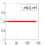
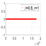
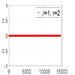
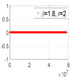
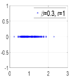
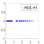
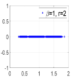
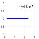
Fig. 1: Eigenvalue distribution of the systems (131) and (132) (for $n=12$) with the single scaling basis functions (first line) and the corresponding multiscale Reisz basis functions (second line), respectively. The horizontal and vertical axes are respectively the real and imaginary axis.

Example 7.2.

We now take $f(x)=1$ in model (3).

If $\lambda=0$, for $x\in\Omega$, the exact solution is $p(x)=\frac{(x-x^{2})^{\beta/2}}{\Gamma(1+\beta)}$ . Although the right-hand side is smooth, $p(x)$ just belongs to $H^{\beta/2+1/2-\epsilon}(\mathbb{R})$ for any $\epsilon>0$. The numerical results are listed in Table 3, where the predicted $1/2-\epsilon$ order of convergence in the $\left\|\cdot\right\|_{H^{\beta/2}(\mathbb{R})}$ norm by Theorem 11 is obtained. The $L^{2}$ convergence orders $(1+\beta)/2$ for $\beta\in(0,1]$ and $1$ for $\beta\in(1,2)$ confirm the result given in [5, Proposition 4.3] for $\lambda=0$. When $\lambda\not=0$, $p(x)$ cannot be obtained explicitly so we list the $\widehat{H}^{\beta/2}$ and $\widehat{L}^{2}$ errors instead, and examine if the convergence rates reflect the convergence rates in the $\left\|\cdot\right\|_{H^{\beta/2}(\mathbb{R})}$ and $\left\|\cdot\right\|_{L^{2}(\mathbb{R})}$ norms, respectively. The numerical results are presented in Table 4, suggesting that the exact solution has a low regularity, but this needs to be confirmed by more in-depth analysis.

Table 3: Numerical results for Example 7.2 with $r=2$ and $\lambda=0$.

$\beta$		$H^{\beta/2}$-Err	Rate	$L^{2}$-Err	rate	$\widehat{H}^{\beta/2}$-Err	Rate	$\widehat{L}^{2}$-Err	Rate
	$8$	9.0822e-02	–	7.8260e-03	–	6.4202e-02	–	5.3795e-03	–
$0.5$	$9$	6.4156e-02	0.50	4.6533e-03	0.75	4.5349e-02	0.50	3.1985e-03	0.75
	$10$	4.5340e-02	0.50	2.7668e-03	0.75	3.2042e-02	0.50	1.9019e-03	0.75
	$8$	4.7148e-02	–	1.1967e-03	–	3.3350e-02	–	7.4060e-04	–
$1.0$	$9$	3.3320e-02	0.50	6.1260e-04	0.97	2.3565e-02	0.50	3.7597e-04	0.98
	$10$	2.3554e-02	0.50	3.1330e-04	0.97	1.6657e-02	0.50	1.9082e-04	0.98
	$8$	2.2624e-02	–	1.7078e-04	–	1.6039e-02	–	9.3174e-05	–
$1.5$	$9$	1.5956e-02	0.50	8.3518e-05	1.03	1.1297e-02	0.50	4.4561e-05	1.06
	$10$	1.1268e-02	0.50	4.1119e-05	1.02	7.9727e-03	0.50	2.1564e-05	1.05

Table 4: Numerical results for Example 7.2 with $r=2$ and $\lambda\not=0$.

	$n$	$\lambda=1.5$				$\lambda=3$
$\beta$		$\widehat{H}^{\beta/2}$-Err	Rate	$\widehat{L}^{2}$-Err	rate	$\widehat{H}^{\beta/2}$-Err	Rate	$\widehat{L}^{2}$-Err	Rate
	$8$	3.1127e-02	–	2.7167e-03	–	4.3713e-02	–	3.9690e-03	–
$0.5$	$9$	2.1930e-02	0.50	1.5970e-03	0.77	3.0757e-02	0.51	2.3121e-03	0.78
	$10$	1.5467e-02	0.50	9.4088e-04	0.76	2.1674e-02	0.50	1.3514e-03	0.77
	$8$	1.6877e-02	–	4.2785e-04	–	2.0984e-02	–	5.8544e-04	–
$1.0$	$9$	1.1972e-02	0.50	2.1812e-04	0.97	1.4924e-02	0.49	2.9984e-04	0.97
	$10$	8.4834e-03	0.50	1.1086e-04	0.98	1.0593e-02	0.49	1.5273e-04	0.97
	$8$	5.8889e-03	–	3.9271e-05	–	6.5308e-03	–	4.7041e-05	–
$1.5$	$9$	4.1724e-03	0.50	1.9185e-05	1.03	4.6490e-03	0.49	2.3304e-05	1.01
	$10$	2.9553e-03	0.50	9.4274e-06	1.02	3.3025e-03	0.49	1.1562e-05	1.01

Example 7.3.

In this example, model (135) is considered in two cases.

For the first case, let $g(x)$ and $f(x)$ in (135) be the functions derived from the postulated exact solution $p(x)=e^{-x^{2}}$. Note that $\mathscr{F}[e^{-x^{2}}](\xi)=\sqrt{\pi}e^{-\xi^{2}/4}$. Then $p(x)\in H^{\mu}(\mathbb{R})$ for any $\mu\geq 0$. The numerical results for $r=1$ and $\eta(x)=S_{1}(x)=\left(e^{-1}-1\right)x+1$ are presented in Figure 2, and show $\frac{2-\beta}{2}$th order convergence in $\left\|\cdot\right\|_{H^{\beta/2}(\mathbb{R})}$ norm and first order convergence in the $\left\|\cdot\right\|_{L^{2}(\mathbb{R})}$ norm.

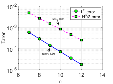
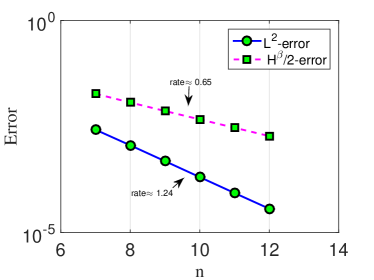
Fig. 2: Numerical results for Example 7.3 with $p(x)=e^{-x^{2}},\,\eta(x)=S_{1}(x)$, and $r=1$. The left one is for $\beta=0.3$ and $\lambda=1.5$, and the right one for $\beta=0.7$ and $\lambda=3$.

For the second case, consider model (135) with the generalized Dirichlet type boundary condition

(150) $$g(x)=\left\{\begin{array}[]{lll}2x-2,&x\in[1,\frac{3}{2}],\\[4.0pt] -2x,&x\in[-\frac{1}{2},0],\\[4.0pt] 0,&x\in(-\infty,-\frac{1}{2})\cup(\frac{3}{2},\infty),\end{array}\right.$$

and the source term $f(x)$ being derived from the exact solution

(155) $$p(x)=\left\{\begin{array}[]{lll}2x-2,&x\in[1,\frac{3}{2}],\\[4.0pt] (x-x^{2})^{2},&x\in(0,1),\\ -2x,&x\in[-\frac{1}{2},0],\\[4.0pt] 0,&{\rm else}.\end{array}\right.$$

Obviously, $p(x)$ does not belong to $H^{\mu}(\mathbb{R})$ for $\mu>1/2$ because of its discontinuity at $x=3/2$ and $x=-1/2$. We consider two different $\eta(x)$, i.e., the $\eta(x)=S_{2}(x)=0$ for $x\in\Omega$, and the $\eta(x)=S_{3}(x)=2x(x-1)$ for $x\in\Omega$. Note that both of them satisfy $\int_{\Omega}\int_{\mathbb{R}}\frac{\left(\eta(x)-\eta(y)\right)^{2}}{|x-y|^{1+\beta}}dxdy<\infty$, required in Theorem 15, but do not belong to $H^{\beta/2}(\mathbb{R})$ (the requirement in [9, Subsection: 4.1]) for $\beta>1$, which implies that the condition in Theorem 15 is weaker than the one of [9, Subsection: 4.1]. The numerical results are presented in Table 5, and also confirm the theoretical prediction of Theorem 16.

Table 5: Numerical results for Example 7.3 with $g(x)$ given as (150) and $r=2$.

$(\eta,\beta)$	$n$	$\lambda=0$				$\lambda=3$
		$H^{\beta/2}$-Err	Rate	$L^{2}$-Err	rate	$H^{\beta/2}$-Err	Rate	$L^{2}$-Err	Rate
	$9$	2.2094e-06	–	1.2913e-07	–	2.2096e-06	–	1.2974e-07	–
$(\eta_{1},0.5)$	$10$	6.5387e-07	1.76	3.2038e-08	2.01	6.5388e-07	1.76	3.2096e-08	2.02
	$11$	1.9393e-07	1.75	7.9785e-09	2.00	1.9393e-07	1.75	7.9839e-09	2.01
	$9$	1.0046e-05	–	5.8314e-07	–	1.0046e-05	–	5.8329e-07	–
$(\eta_{2},0.5)$	$10$	2.9847e-06	1.75	1.4573e-07	2.00	2.9847e-06	1.75	1.4574e-07	2.00
	$11$	8.8697e-07	1.75	3.6426e-08	2.00	8.8697e-07	1.75	3.6427e-08	2.00
	$9$	1.3532e-05	–	1.3167e-07	–	1.3532e-05	–	1.3623e-07	–
$(\eta_{1},1.0)$	$10$	4.7735e-06	1.50	3.2397e-08	2.02	4.7734e-06	1.50	3.3008e-08	2.04
	$11$	1.6846e-06	1.50	8.0282e-09	2.01	1.6846e-06	1.50	8.1080e-09	2.02
	$9$	6.1750e-05	–	5.8376e-07	–	6.1750e-05	–	5.8506e-07	–
$(\eta_{2},1.0)$	$10$	2.1824e-05	1.50	1.4581e-07	2.00	2.1824e-05	1.50	1.4597e-07	2.00
	$11$	7.6881e-06	1.51	3.6437e-08	2.00	7.6881e-06	1.51	3.6457e-08	2.00
	$9$	1.7807e-04	–	1.8024e-07	–	1.7807e-04	–	1.9737e-07	–
$(\eta_{1},1.6)$	$10$	7.7452e-05	1.20	4.2847e-08	2.07	7.7452e-05	1.20	4.6850e-08	2.07
	$11$	3.3700e-05	1.20	1.0224e-08	2.06	3.3700e-05	1.20	1.1129e-08	2.07
	$9$	8.1486e-04	–	6.1682e-07	–	8.1486e-04	–	6.4349e-07	–
$(\eta_{2},1.6)$	$10$	3.5467e-04	1.20	1.5186e-07	2.02	3.5467e-04	1.20	1.5665e-07	2.04
	$11$	1.5438e-04	1.20	3.7543e-08	2.01	1.5438e-04	1.20	3.8407e-08	2.03

8 Conclusions

We have presented Riesz basis Galerkin methods for effectively solving the tempered fractional Laplacian equation, where the operator is the generator of the tempered $\beta$-stable Lévy process. The well-posedness of the equation and convergence of the scheme were theoretically proved. When $\lambda=0$, the model reduces to a fractional Laplacian equation and the present theoretical framework is still valid. We also discussed efficient implementations of our methods, including the generation of stiff matrix and the effectiveness of multiscale preconditioning. We performed several numerical simulations to confirm the theoretical results and demonstrate the high efficiency of the schemes. The present work is confined to one dimensional problems with basis functions on uniform meshes. The generalization to higher dimensions and the approximation with locally refined basis functions are very important topics and will be considered in future work.

Appendix A Proof of $\mathcal{G}(\lambda,\xi,\beta)\geq 0$

Proof.

By (31), it is easy to check that this proof is equivalent to show that

$$f(t)=(-1)^{\lfloor\beta\rfloor}\left(\cos\Big{(}\beta\arctan(t)\Big{)}-\frac{1}{\left(1+t^{2}\right)^{\beta/2}}\right)\geq 0$$

for $\beta\in(0,1)\cup(1,2)$, and

$$g(t)=t\arctan(t)-\frac{1}{2}\ln(1+t^{2})\geq 0$$

for $\beta=1$, where $t=\frac{|\xi|}{\lambda}\in[0,\infty)$. For $\beta=1$, we have $g^{\prime}(t)=\arctan(t)\geq 0$, so $g(t)\geq g(0)=0$. For $\beta\in(0,1)\cup(1,2)$, there exists

$$f^{\prime}(t)=(-1)^{\lfloor\beta\rfloor}\frac{\beta}{1+t^{2}}\left(-\sin\Big{(}\beta\arctan(t)\Big{)}+\frac{t}{(1+t^{2})^{\frac{\beta}{2}}}\right).$$

Thus if $0<\beta<1$, we have

$$f^{\prime}(t)\geq(-1)^{\lfloor\beta\rfloor}\frac{\beta}{1+t^{2}}\left(-\sin\Big{(}\arctan(t)\Big{)}+\frac{t}{(1+t^{2})^{\frac{1}{2}}}\right)=0.$$

Then $f(t)\geq f(0)=0$ for $\beta\in(0,1)$. If $1<\beta<2$, we have

$$f^{\prime}(t)=(-1)^{\lfloor\beta\rfloor}\Bigg{(}-\sin\Big{(}(\beta-1)\arctan(t)\Big{)}\cos\Big{(}\arctan(t)\Big{)}$$

$$~{}~{}-\frac{t}{(1+t^{2})^{\frac{1}{2}}}\bigg{(}\cos\Big{(}(\beta-1)\arctan(t)\Big{)}-\frac{1}{\left(1+t^{2}\right)^{\frac{\beta-1}{2}}}\bigg{)}\Bigg{)}\geq 0,$$

where the result $f(t)\geq 0$ for $\beta\in(0,1)$ has been used to justify the nonnegativity. Then $f(t)\geq f(0)=0$ for $\beta\in(1,2)$. ∎

References

- [1] G. Acosta, F. Bersetche, and J. P. Borthagaray, A short FE implementation for a d homogeneous Dirichlet problem of a fractional Laplacian, Comput. Math. Appl., 74 (2017), pp. 784-816.
- [2] G. Acosta and J. P. Borthagaray, A fractional Laplace equation: regularity of solutions and finite element approximations, SIAM J. Numer. Anal., 55 (2017), pp. 472-495.
- [3] M. Abramowitz and I. A. Stegun, Handbook of Mathematical Functions, Dover Publications, 1965, Chapter 5.
- [4] B. Baeumer and M. M. Meerschaert, Tempered stable Lévy motion and transient super-diffusion, J. Comput. Appl. Math., 233 (2010), pp. 2438–2448.
- [5] J. P. Borthagaray, L. M. Del Pezzo, and S. Martinez, Finite element approximation for the fractional eigenvalue problem, arXiv:1603.00317 (2016).
- [6] S. C. Brenner and L. R. Scott, The Mathematical Theory of Finite Element Methods, Second-Edition, Springer-Verlag, New York, 2002.
- [7] H. F. Chan and X. Q. Jin, An Introduction to Iterative Toeplitz Solvers, SIAM, Philadelphia, PA, 2007.
- [8] A. Cohen, Wavelet methods in numerical analysis, in Handbook of Numerical Analysis, P. Ciarlet, J. Lions eds. Elsevier North-Holland, 2000, pp. 417–711.
- [9] W. H. Deng, B. Y. Li, W. Y. Tian, and P. W. Zhang, Boundary problems for the fractional and tempered fractional operators, Multiscale Model. Simul., in press, 2017.
- [10] W. H. Deng and Z. J. Zhang, Numerical schemes of the time tempered fractional Feynman-Kac equation, Comput. Math. Appl., 73 (2017), pp. 1063–1076.
- [11] M. D’Elia and M. Gunzburger, The fractional Laplacian operator on bounded domains as as a special case of the nonlocal diffusion operator, Comput. Math. Appl., 66 (2013), pp. 1245–1260.
- [12] Q. Du, M. Gunzburger, R. B. Lehoucq, and K. Zhou, Analysis and approximation of nonlocal diffusion problems with volume constraints, SIAM. Review, 54 (2012), pp. 667–696.
- [13] B. Dyda, A fractional order Hardy inequality, Illinois J. Math., 48 (2004), pp. 575–588.
- [14] V. J. Ervin, N. Heuer, and J. P. Roop, Regularity of the solution to -D fractional order diffusion equations, arXiv:1608.00128v1 (2016).
- [15] A. Fiscella, R. Servadei, and E. Valdinoci, Density properties for fractional Sobolev spaces, Ann. Acad. Sci. Fenn. Math., 40 (2015), pp. 235-253.
- [16] I. S. Gradshteyn, I. M. Ryzhik, Y. V. Geraniums, and M. Y. Tseytlin, Table of Integrals, Series, and Products, A. Jeffrey, ed., Translated by Scripta Technica, Academic Press, USA, 1980.
- [17] G. Guo, X. K. Pu, and F. H. Huang, Fractional Partial Differential Equations and Their Numerical Solutions, World Scientific, Singapore, 2015.
- [18] E. Hanert and C. Piret, A Chebyshev pseudospectral method to solve the space-time tempered fractinal diffusion equation, SIAM J. Sci. Comput., 36 (2015), pp. A1797–A1812.
- [19] Y. Huang and A. M. Oberman, Numerical methods for the fractional Laplacian: A finite difference-quadrature approach, SIAM J. Numer. Anal., 52 (2014), pp. 3056–3084.
- [20] R. Q. Jia, Spline wavelets on the interval with homogeneous boundary conditions, Adv. Comput. Math., 30 (2009), pp. 177–200.
- [21] B. T. Jin, R. Lazarov, J. Pasciak, and W. Runadell, Variational formulation of problems involving fractional order differential operators, Math. Comp., 84 (2015), pp. 2665–2700.
- [22] C. Li and W. H. Deng, High order schemes for the tempered fractional diffusion equations, Adv. Comput. Math., 42 (2016), pp. 543–572.
- [23] M. Loss and C. Sloane, Hardy inequalities for fractional integrals on general domains, J. Funct. Anal., 259 (2010), pp. 1369–1379.
- [24] W. McLean, Strongly Elliptic Systems and Boundary Integral Equations, Combridge university press, Cambrige, 2000.
- [25] R. Metzler and J. Klafter, The random walk’s guide to anomalous diffusion: a fractional dynamics approach, Phys. Rep., 339 (2000), pp. 1-77.
- [26] C. Pozrikidis, The Fractional Laplacian, CRC Press, London, 2016.
- [27] M. Primbs, New stable biorthogonal spline wavelets on the interval, Results. Math, 57 (2010), pp. 121–162.
- [28] J. Shen, T. Tang and L. L, Wang, Spectral Methods: Algorithms, Analysis and Applications, Springer, New York, 2011.
- [29] X. C. Tian, Q. Du, and M. Gunzburger, Asymptotically compatible schemes for the approximation of fractional Laplacian and related nonlocal diffusion problems on bounded domains, Adv. Comput. Math., 42 (2016), pp. 1363–1380.
- [30] K. Urban, Wavelet Methods for Elliptic Partial Differential Equations, Oxford University Press, Oxford, 2009.
- [31] H. Wang, K. Wang, and T. Sircar, A direct finite difference method for fractional diffusion equations, J. Comput. Phys., 229 (2010), pp. 8095-8104.
- [32] Q. W. Xu and J. S. Hesthaven, Discontinuous Galerkin method for fractional convection-dissuion equations, SIAM. J. Numer. Anal., 52 (2014), pp. 405–423.
- [33] M. Zayernouri, M. Ainsworth, and G.E. Karniadakis, Tempered fractional Sturm-Liouville eigenproblems, SIAM J. Sci. Comput., 37 (2015), pp. A1777–A1800.
- [34] Z. J. Zhang and W. H. Deng, Numerical approaches to the functional distribution of anomalous diffusion with both traps and flights, Adv. Comput. Math., 43 (2017), pp. 699–732.