Nodal statistics on quantum graphs

Abstract.

It has been suggested that the distribution of the suitably normalized number of zeros of Laplacian eigenfunctions contains information about the geometry of the underlying domain. We study this distribution (more precisely, the distribution of the “nodal surplus”) for Laplacian eigenfunctions of a metric graph. The existence of the distribution is established, along with its symmetry. One consequence of the symmetry is that the graph’s first Betti number can be recovered as twice the average nodal surplus of its eigenfunctions. Furthermore, for graphs with disjoint cycles it is proven that the distribution has a universal form — it is binomial over the allowed range of values of the surplus. To prove the latter result, we introduce the notion of a local nodal surplus and study its symmetry and dependence properties, establishing that the local nodal surpluses of disjoint cycles behave like independent Bernoulli variables.

1. Introduction

Studying various properties of the nodal sets of Laplacian eigenfunctions is a subject with a long history in mathematical physics. The number of the zeros or the nodal domains (depending on the context and the dimension) of the $n$-th eigenfunction is one of the simplest quantities one can observe experimentally. Yet, analytical study of this quantity as a function of $n$ is complicated by its non-locality, which can be appreciated by observing that different nodal domains of the same eigenfunction can vary wildly in size and shape. Classical results in estimating this number include those of Sturm [56], Courant [22] and Pleijel [49], with notable recent contributions by Ghosh, Reznikov and Sarnak [30] and by Jung and Zelditch [36, 35]. In a series of works of Smilansky and co-authors [17, 34, 33, 31, 6, 37, 5] it has also been proposed that studying the distribution of the appropriately rescaled number of nodal domains can reveal much about the geometry of the underlying system. This line of thought has lead to such results as the Bogomolny and Schmit [18] prediction for the average number of the nodal domains (by analogy with a percolation model), a proof by Nazarov and Sodin [48] that the average rescaled number of the nodal domains for random waves is non-zero, as well as a slew of high-precision numerical studies [47, 39, 8].

In this paper we will investigate the distribution of the nodal count of Laplacian eigenfunctions on metric graphs, a class of models which was used to study the nodal count distributions from the very start [34, 6, 5]. We will show, first of all, that the statistical distribution of the nodal count is a well defined object. The nodal count of the $n$-th eigenfunction, when shifted down by $n-1$, takes values in a bounded range of integers; we call the shifted count the nodal surplus. For any graph we will show that the limiting frequency of the appearance of a given surplus in the spectral sequence can be calculated as an integral of a piecewise constant function over an analytic subvariety of a torus which is called secular manifold.

The nodal count distribution is shown to be symmetric around its mean, which is equal to half the first Betti number $\beta$ of the graph; conversely, the first Betti number can be recovered from the nodal statistics. Furthermore, for a class of graphs whose cycles are disjoint, we will prove that, despite knowing neither the individual eigenvalues nor the zero count of individual eigenfunctions, we can predict the limiting nodal count distribution. It takes a universal form — the binomial distribution over the a priori allowed range of values, from 0 to $\beta$.

To prove the latter, we introduce a new concept of a local nodal surplus. That such a quantity can be defined at all is very interesting in itself, due to the issue of non-locality mentioned above. To explain this concept informally, recall that the global nodal surplus can be viewed as a deviation of the number of zeros from the baseline $n-1$, attributable to the presence of cycles in the graph. One therefore expects that the extra number of zeros is “localized” on the cycles and, if the graph has block structure (can be disconnected by cutting bridges, for example), one should be able to talk about the local nodal surplus of an individual block. This notion will be rigorously defined in this paper by analytic means. Its geometric meaning is far from obvious: the global nodal surplus is the difference between the number of zeros and $n-1$, and while the local meaning of the number of zeros is obvious enough, there is no local analogue of the eigenfunction’s number $n$. Our analytic definition, however, allows us to prove that for a graph with disjoint cycles, the local surpluses of the cycles behave like independent Bernoulli variables, hence the binomial distribution of the global nodal surplus.

2. Definitions and Main Results

Let $\Gamma\left(\mathcal{V},\mathcal{E},l\right)$ be a finite connected metric graph with a set of vertices $\mathcal{V}$ and a set of edges $\mathcal{E}$. The sizes of the sets $\mathcal{V}$ and $\mathcal{E}$ are denoted $V$ and $E$ correspondingly. The last entry of the triple is the length function $l:\mathcal{E}\to\mathbb{R}_{+}$ which associates to each edge $e\in\mathcal{E}$ a positive length which we will denote $l_{e}$. We will identify each edge with an interval $[0,l_{e}]$ of the corresponding length. In doing so one needs to choose an orientation for the edge, but this can be done arbitrarily and does not affect the results in any way. Note that we allow multiple edges between the same pair of vertices and also edges with both ends at the same vertex (loops).

A quantum graph is a metric graph $\Gamma\left(\mathcal{V},\mathcal{E},l\right)$ equipped with a Schrödinger type operator acting on the Hilbert space $\bigoplus_{e\in E}L^{2}([0,l_{e}])$ with a suitable domain. We will not consider potentials, restricting our attention to Laplace operator

(1) $$\mathcal{H}=-\Delta,\qquad\mathcal{H}:\,f\mapsto-\frac{d^{2}f}{dx_{e}^{2}}.$$

The magnetic Schrödinger operator will also play an important role; we will define it in Section 3.1.

In this paper we will consider the most common vertex conditions for which these operators are self-adjoint. We say that a function obeys the Neumann boundary conditions if at any vertex $v\in\mathcal{V}$ it is continuous and

(2) $$\sum_{e\in E_{v}}\frac{d}{dx}f(v)=0$$

where $E_{v}$ is the set of edges incident to the vertex $v$, and by convention the derivatives are taken into the edge $e$. At a vertex of degree one, the above conditions reduce to the standard Neumann condition $f^{\prime}(v)=0$. At such vertices we will also allow Dirichlet conditions (i.e. $f(v)=0$). A connected quantum graph different from a circle or a polygon and with the above vertex conditions will be called a nontrivial standard graph.

Further details about theory of quantum graphs can be found in the books [32, 12, 46] as well as the recent elementary notes [11].

2.1. The nodal surplus

Since our quantum graph is compact, the operator $\mathcal{H}$ has a discrete spectrum of eigenvalues $\left\{\lambda_{n}\right\}_{n=1}^{\infty}$ and corresponding eigenfunctions $\left\{f_{n}\right\}_{n=1}^{\infty}$. For the operators presented here, the spectrum is non-negative, and we will use the notation $\lambda_{n}=k_{n}^{2}$. From here on we will also refer to $k_{n}\geq 0$ as the eigenvalue of the graph. The eigenfunctions of (1) can be chosen to be real and, if the eigenfunction does not vanish on entire edges (which is possible on graphs due to failure of unique continuation principle), one can count the number of the zeros of the $n$-th eigenfunction. This quantity will be denoted by $\phi_{n}$ and will be the main object of our study.

From now on we will call $k_{n}$ and $f_{n}$ generic eigenvalue and eigenfunction if the eigenvalue $k_{n}$ is simple and the eigenfunction $f_{n}$ does not vanish on the vertices (and therefore edges) of the graph. We will routinely assume that the edge lengths are independent over the field $\mathbb{Q}$ of rational numbers (or rationally independent). This will be shown to guarantee that a majority of the eigenvalues are generic (see [27, 14] and Appendix A). Furthermore, if the graph has no loops, for a choice of rationally independent edge lengths all eigenvalues are generic, hence the name.

The nodal count of a tree graph is $\phi_{n}=n-1$ which is a generalization of Sturm’s oscillation theorem that was obtained in [50, 53] (interestingly, the converse result has also been established [1]: if the nodal count is $\phi_{n}=n-1$ then the graph is a tree). For graphs which are not trees $n-1$ provides a baseline from which the actual number of zeros does not stray very far. Defining the $n$-th nodal surplus by $\sigma_{n}=\phi_{n}-(n-1)$ we have the following bounds

(3) $$0\leq\sigma_{n}\leq\beta,$$

where $\beta$ is the number of independent cycles on the graph (i.e. the number of generators of the first homology group of the graph — the first Betti number), and is equal to

(4) $$\beta=E-V+1.$$

We remark that the $1$ above stands for the number of connected components of the graph. The upper bound was proven in [34] and the lower bound in [9] (see also [3]).

An interesting insight on the nature of these bounds comes from the characterization of the nodal surplus in terms of the Morse index of the eigenvalue as a function of certain parameters [10, 19, 15]. This theorem will play a central role in our study and we review it in Section 3.1.

2.2. Main Results

In order to investigate the nodal surplus of a graph we wish to define a surplus distribution that will give the density of a given value in the nodal surplus sequence.

Theorem 2.1.

Let $\Gamma$ be a nontrivial standard graph with rationally independent lengths. Then the nodal surplus distribution of $\Gamma$ is a well defined probability distribution on the set $\{0,1,\ldots,\beta\}$ given by

(5) $$p_{s}=\lim_{N\to\infty}\frac{\left|\left\{n\in\mathcal{G}_{N}|\,\sigma_{n}=s\right\}\right|}{\left|\mathcal{G}_{N}\right|},\qquad 0\leq s\leq\beta,$$

where $\mathcal{G}_{N}$ is the set of indices $1\leq n\leq N$ such that $k_{n}$ is generic. Furthermore, the distribution is symmetric, in the sense that

(6) $$p_{s}=p_{\beta-s},\quad 0\leq s\leq\beta,$$

and, therefore, the value of $\beta$ can be recovered as twice the average nodal surplus

(7) $$\beta=2\,\mathbb{E}(\sigma_{n}):=\lim_{N\to\infty}\frac{2}{\left|\mathcal{G}_{N}\right|}\sum_{n\in\mathcal{G}_{N}}\sigma_{n}.$$

Remark 2.2.

Equation (7) generalizes the inverse result of [1]: $p_{0}=1$ implies $\beta=0$.

Figure 1. An example of a graph with five disjoint cycles.

We now define the special structure of the graphs where we can say more about the form of the distribution $p_{s}$. A simple cycle in the graph $\Gamma$ is a sequence of vertices $[v_{1},\ldots,v_{k}]$, such that there is an edge connecting vertex $v_{j}$ to $v_{j+1}$ for all $j$ (including $v_{k}$ to $v_{1}$) and no vertex appears more than once. A graph is said to have disjoint cycles if there is a basis set of $\beta$ cycles such that each vertex $v\in\mathcal{V}$ is traversed by at most one cycle, see Figure 1 for an example.

Theorem 2.3.

Let $\Gamma$ be a nontrivial standard graph with rationally independent lengths. If the cycles of $\Gamma$ are disjoint, then the nodal surplus distribution of $\Gamma$ is Binomial with parameters $\beta$ and $1/2$. That is,

(8) $$p_{s}=\frac{1}{2^{\beta}}\binom{\beta}{s},\qquad 0\leq s\leq\beta.$$

Our approach to analyzing the nodal surplus sequence $\{\sigma_{n}\}$ is interpreting it as a sample of a certain function defined on a certain manifold endowed with a probability measure. The manifold and the measure go back to an idea of Barra and Gaspard [7]; the fact that the nodal surplus can be read off the manifold was shown by Band [1] who converted the nodal-magnetic connection of Berkolaiko and Weyand [15] into a function on the manifold. Existence of the limit in (5) follows from the ergodicity of the sampling process (which goes back to Weyl [59]). The symmetry (6) is a consequence of a simple symmetry of the nodal surplus function, the underlying manifold and the measure.

Our second main result requires a much more detailed analysis of the manifold and the nodal surplus function. Considering a more general situation, a graph consisting of disjoint blocks of cycles, we show that the total nodal surplus is a sum of the “local surpluses” of individual blocks. These local surpluses also have symmetry similar to (6), but with $\beta$ equal to the number of cycles in their block. Moreover this symmetry is independent of the values taken by other local surpluses. If each block has just one cycle, the local surpluses become independent (rather than merely “independently symmetric”), thus producing the binomial distribution.

Our proofs require several technical tools and results. To avoid tiring the reader we describe these results on the “as needed” basis. Section 3 introduces magnetic Laplacian, the magnetic-nodal connection, secular equation and secular manifold, and the Barra-Gaspard measure before proceeding to prove Theorem 2.1. Section 4 defines the notion of a block of a graph, introduces scattering from a graph, a factorization of the secular equation by splitting a graph into two parts, defines the local nodal surplus and studies its properties, culminating in a proof of Theorem 2.3. In Appendices A, B and C we prove some auxiliary results used in the paper. Finally (and perhaps most interestingly for readers looking for open problems), in Appendix D we present some simple examples of nodal surplus distributions, both numerical and analytical, mostly of the graphs falling outside the assumptions of Theorem 2.3. This helps us to understand to what extent the assumptions are optimal.

3. Defining the distribution

To get an analytic handle on the nodal distribution we combine two techniques of quantum graphs analysis: the magnetic-nodal connection of Berkolaiko, Colin de Verdière and Weyand [10, 19, 15] and the secular manifold of Barra and Gaspard [7] further developed in [16, 2, 20]. We lay out the required foundations in the next subsections.

3.1. The magnetic Laplacian and the magnetic-nodal connection

The magnetic Laplacian is the operator on $\bigoplus_{e\in E}L^{2}([0,l_{e}])$ acting as

(9) $$\mathcal{H}_{A}:f\mapsto\left(i\frac{d}{dx}+A(x)\right)^{2}f,$$

where $A(x)$ is a piecewise continuous 1-form called the magnetic potential. The vertex conditions are modified by substituting (2) with

(10) $$\sum_{e\in E_{v}}\left(i\frac{d}{dx}+A(x)\right)f(v)=0.$$

Naturally, when $A\equiv 0$ we recover the non-magnetic Laplacian of (1).

A magnetic flux of a magnetic potential $A$ through an oriented cycle $\gamma$ is defined as

(11) $$\alpha_{\gamma}:=\left[\oint_{\gamma}A(x)\right]\mod 2\pi.$$

The fluxes through independent cycles of the graph $\Gamma$ completely determine the magnetic Laplacian in the following sense.

Lemma 3.1.

Two magnetic Laplacian operators $\mathcal{H}_{A},\mathcal{H}_{A^{\prime}}$ are unitarily equivalent if the magnetic potentials $A$ and $A^{\prime}$ have the same flux through every cycle $\gamma$.

The above lemma is well-known with proofs in the quantum graph setting appearing, for example, in [42, 15]. Due to additivity of fluxes, it is enough to know them for a fundamental set of cycles, $\beta$ in number. Fixing a particular fundamental set of cycles (together with orientation) we collect the corresponding fluxes into the flux vector $\vec{\alpha}\in\mathbb{T}^{\beta}$. Here $\mathbb{T}^{\beta}$ is the $\beta$-dimensional flat torus $\mathbb{R}^{\beta}/(2\pi\mathbb{Z})^{\beta}$.

We can thus speak of the eigenvalues of the “operator” $\mathcal{H}^{\vec{\alpha}}$ (which is actually an equivalence class of operators $\mathcal{H}_{A}$). Consider these eigenvalues $\left\{k_{n}\left(\vec{\alpha}\right)\right\}_{n=1}^{\infty}$ as functions of the fluxes $\vec{\alpha}$. At the point $\vec{\alpha}=0$ they are equal to the eigenvalues of the non-magnetic operator $\mathcal{H}$. What is far from obvious is that the behavior of $k_{n}(\vec{\alpha})$ around $\vec{\alpha}=0$ determines the nodal surplus of the $n$-th eigenfunction of $\mathcal{H}$.

Theorem 3.2 (Berkolaiko–Weyand [15]).

Let $\Gamma$ be a quantum graph, $k_{n}>0$ a generic eigenvalue of $\mathcal{H}$ on $\Gamma$ and $\sigma_{n}$ its nodal surplus. Consider the eigenvalue $k_{n}(\vec{\alpha})$ of the corresponding magnetic Schrödinger operator as a function of $\vec{\alpha}$. Then $\vec{\alpha}=0$ is a smooth non-degenerate critical point of $k_{n}\left(\vec{\alpha}\right)$ and its Morse index is equal to the nodal surplus $\sigma_{n}$.

The Morse index of a function is the number of negative eigenvalues of the Hessian evaluated at a critical point of this function. Because Hessians will play a large role in our proofs, we should set up notation carefully.

Definition 3.3.

Let $f(\vec{x},\vec{y})$ be a twice differentiable function of a finite number of variables $\vec{x}=(x_{1},\ldots,x_{n})$ and $\vec{y}=(y_{1},\ldots,y_{m})$. The Hessian of $f$ with respect to variables $\vec{y}$ evaluated at the point $\vec{x}=\vec{x}^{*}$ and $\vec{y}=\vec{y}^{*}$ is a matrix of second derivatives

(12) $$H_{\vec{y}}(f)(\vec{x}^{*},\vec{y}^{*}):=\left[\frac{\partial^{2}f}{\partial y_{i}\partial y_{j}}(\vec{x}^{*},\vec{y}^{*})\right]_{i,j=1}^{m}.$$

For a symmetric matrix $A$ we will denote by $\mathcal{M}[A]$ the number of its negative eigenvalues (Morse index).

With this notation in hand, Theorem 3.2 can be summarized as

(13) $$\sigma_{n}=\mathcal{M}\left[H_{\vec{\alpha}}(k_{n})\left(\vec{0}\right)\right],$$

where $k_{n}=k_{n}\left(\vec{\alpha}\right)$.

3.2. Bond scattering matrix and secular equation.

Solving the eigenvalue equation $\mathcal{H}_{A}f=k^{2}f$ for $k>0$ on every edge and applying the vertex condition we arrive at the secular equation on the eigenvalues $k$ [58, 44, 43]. In this subsection we review this procedure.

Taking, without loss of generality, the magnetic potential to be constant on each edge, the solution on the edge $e$ is given by

(14) $$f(x_{e})=a_{e}e^{-i(k+A_{e})(l_{e}-x_{e})}+a_{\hat{e}}e^{-i(k-A_{e})x_{e}}.$$

Thus each edge corresponds to two “directed” coefficients, $a_{e}$ and $a_{\hat{e}}$, which can be viewed as the amplitudes of waves traveling in and against the chosen direction of $e$. The label $\hat{e}$ is called the reversal of the (label) $e$. The hat can be viewed as a permutation (fixed-point free involution) on the set of labels if we extend it by $\hat{\hat{e}}=e$. If we introduce variables $x_{\hat{e}}:=L-x_{e}$ and $A_{\hat{e}}=-A_{e}$, expression (14) becomes nicely symmetric.

Let us fix a particular representative of the equivalence class of operators $\mathcal{H}_{A}$ (see [15] for more detail). Choose a set $\mathcal{C}$ of $\beta$ edges whose removal from $\mathcal{E}$ does not disconnect the graph. The remaining graph is a spanning tree. We set the magnetic potential to be non-zero only on the edges $e_{j}\in\mathcal{C}$, with $A_{e_{j}}=\alpha_{j}/l_{e_{j}}$.

Assume $f$ is an eigenfunction of $\mathcal{H}_{A}$ corresponding to the eigenvalue $k>0$. According to (14), $f$ is uniquely determined by a vector of coefficients

(15) $$\vec{a}\in\mathbb{C}^{2E},\qquad\vec{a}=\left(a_{1},a_{\hat{1}},...,a_{E},a_{\hat{E}}\right).$$

Note that we have chosen a specific order of the edge labels. Imposing the vertex conditions on $f$ and simplifying the result we arrive to the condition

(16) $$\left(\boldsymbol{I}-e^{i\boldsymbol{\alpha}}e^{ik\boldsymbol{L}}\boldsymbol{S}\right)\vec{a}=0,$$

where $\boldsymbol{L}$ is the diagonal matrix of the edge lengths and $\boldsymbol{\alpha}$ is the diagonal matrix of edge-integrated magnetic potential values, which in our chosen representation of potential are given by 0, $\alpha_{e}$ or $\alpha_{\hat{e}}=-\alpha_{e}$. Assuming for the moment that the edges in $\mathcal{C}$ are the first in the order established by (15), we have

$$\boldsymbol{L}=\operatorname{diag}(l_{1},l_{1},l_{2},l_{2},\ldots,l_{E},l_{E})\qquad\boldsymbol{\alpha}=\operatorname{diag}(\alpha_{1},-\alpha_{1},\alpha_{2},-\alpha_{2},\ldots,0,0).$$

The matrix $\boldsymbol{S}$ (called the bond-scattering matrix) is unitary. For a graph with Neumann (or Dirichlet) vertex conditions it has constant coefficients given by the following rules. Let $e$ be the label corresponding to a directed edge terminating at vertex $v$ and let $\deg(v)$ denote the degree of the vertex $v$. Then the elements of $\boldsymbol{S}$ are

(17) $$S_{e^{\prime},e}=\begin{cases}\frac{2}{\deg(v)}-1,&\mbox{if }e^{\prime}=\hat{e},\\ \frac{2}{\deg(v)},&\mbox{if $d^{\prime}$ originates at $v$ and }e^{\prime}\neq\hat{e},\\ 0&\mbox{otherwise}.\end{cases}.$$

Finally, if we choose to impose Dirichlet condition at a vertex $v$ of degree 1 then the corresponding element of $\boldsymbol{S}$ changes from $1$ given by (17) to $-1$.

It is an explicit computation that each term in the product $e^{i\boldsymbol{\alpha}}e^{ik\boldsymbol{L}}\boldsymbol{S}$ is a unitary matrix. The multiplicity of $k^{2}\neq 0$ as an eigenvalue in the spectrum of $\mathcal{H}$ is equal to the dimension of the kernel of $\boldsymbol{I}-e^{i\boldsymbol{\alpha}}e^{ik\boldsymbol{L}}\boldsymbol{S}$. In other words, the geometric multiplicity of $k^{2}$ is equal to the algebraic multiplicity of $k>0$ as the root of the secular equation

(18) $$\tilde{F}\left(k;\vec{\alpha}\right):=\det\left(\boldsymbol{I}-e^{i\boldsymbol{\alpha}}e^{ik\boldsymbol{L}}\boldsymbol{S}\right)=0,$$

For more complete understanding of the scattering approach we refer the reader to [12, 32].

3.3. The torus flow

We now describe an approach pioneered by Barra and Gaspard [7] in their study of eigenvalue spacing of small quantum graphs.

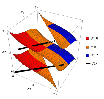
(a) (b)

Figure 2. (a) The torus flow defined by (20) hits the secular manifold. The values of $k$ for which this happens are the eigenvalues of the graph. The secular manifold in the figure is of the “dumbbell graph” graph as analyzed in Appendix D.2. The secular manifold is colored according to the values of the nodal surplus function, equation (24). (b) The “dumbbell” graph with torus coordinates marked on corresponding edges.

Let $\Gamma$ be a metric graph and define

(19) $$F:\mathbb{T}^{E}\times\mathbb{T}^{\beta}\to\mathbb{C},\qquad F\left(\vec{\varkappa};\vec{\alpha}\right)=\det\left(\boldsymbol{I}-e^{i\boldsymbol{\alpha}}e^{i\boldsymbol{x}}\boldsymbol{S}\right),$$

where $\boldsymbol{S}$ has been calculated according to prescription (17) and

$$\boldsymbol{x}=\operatorname{diag}\left(x_{1},x_{1},...x_{E},x_{E}\right).$$

Consider the linear flow on the torus $\mathbb{T}^{E}$

(20) $$\varphi:\mathbb{R}\rightarrow\mathbb{T}^{E},\qquad\varphi\left(k\right)=k\vec{l}\mod 2\pi,$$

where $\vec{l}=(l_{1},\ldots,l_{E})$ is the vector of lengths of $\Gamma$. Observe that

(21) $$\tilde{F}\left(k;\vec{\alpha}\right)=F\left(\varphi(k);\vec{\alpha}\right).$$

For the rest of the paper, $F$ will be referred to as the secular function of $\Gamma$. Define the secular manifold,

(22) $$\Sigma:=\left\{\vec{\varkappa}:F\left(\vec{\varkappa};0\right)=0\right\}\subset\mathbb{T}^{E}$$

(note that it is a slight misnomer, as generally $\Sigma$ is an algebraic variety with singularities and not a smooth manifold). The spectrum of $\mathcal{H}$ on $\Gamma$ can be described as the values of $k$ for which the flow $\phi$ hits the secular manifold,

(23) $$\left\{k_{n}\right\}_{n=1}^{\infty}\setminus\{0\}=\left\{k>0:\varphi(k)\in\Sigma\right\},$$

see Figure 2 for an example. Moreover, the multiplicity of the eigenvalue $k$ is the same as the algebraic multiplicity of the root $\vec{\varkappa}=\varphi(k)$ of $F(\vec{\varkappa};0)$. We remark that we took some pains to exclude zero eigenvalue from (23). Zero may or may not be an eigenvalue of the graph (it is not an eigenvalue if we have some Dirichlet vertices), and in general its multiplicity is different from the multiplicity of $\vec{\varkappa}=\vec{0}$ as a root of $F(\vec{\varkappa};0)$; this topic is studied in some detail in [28].

We can similarly define $\Sigma(\vec{\alpha})$ whose piercings by the flow will give the eigenvalues $k_{n}\left(\vec{\alpha}\right)$ of the magnetic operator.

A surprising consequence of Theorem 3.2, pointed out in [1], is that one can read off the nodal surplus information directly off the secular manifold $\Sigma$.

Theorem 3.4.

For a graph $\Gamma$, define the nodal surplus function by

(24) $$\sigma:\Sigma\to\{0,\ldots,\beta\}\qquad\sigma\left(\vec{\varkappa}\right):=\mathcal{M}\left[-\frac{H_{\vec{\alpha}}(F)\left(\vec{\varkappa};\vec{0}\right)}{\nabla_{\varkappa}F\cdot\vec{l}}\right].$$

Then the function $\sigma$ is independent of $\vec{l}$ and if $k_{n}>0$ is generic, it gives the nodal surplus of the corresponding eigenfunction,

(25) $$\sigma\left(k_{n}\vec{l}\right)=\sigma_{n}.$$

See Figure 2(a) for a demonstration of the nodal surplus function for a particular graph.

Remark 3.5.

Before we sketch the proof of the Theorem, let us discuss its significance. We have defined an “oracle” function which calculates the nodal surplus from $\vec{\varkappa}$ alone. For different choices of $\vec{l}$ a given point $\vec{\varkappa}\in\Sigma$ may be reached by the flow $\varphi(k)$ at very different values of $k$, if it is reached at all. The corresponding eigenfunctions have very different numbers of zeros and come at different sequence numbers in the spectrum of their graph, yet the nodal surplus remains the same!

Proof of Theorem 3.4.

Equation (25) follows directly from Theorem 3.2 by calculating the Hessian in terms of the function $F$,

$$H_{\vec{\alpha}}(k_{n})\left(\vec{0}\right)=-\frac{H_{\vec{\alpha}}(F)\left(\vec{\varkappa};\vec{0}\right)}{\nabla_{\varkappa}F\cdot\vec{l}}.$$

This was performed in [1], where it was also pointed out that $\nabla_{\varkappa}F$ has all entries of the same sign (up to an overall phase) or $0$. Moreover, if $k_{n}$ is simple then at $\vec{\varkappa}=k_{n}\vec{l}$ the gradient $\nabla_{\varkappa}F\neq 0$, so the function $\sigma$ is well defined. Since only the sign of $\nabla_{\varkappa}F\cdot\vec{l}$ is important in calculating the Morse index, and $\vec{l}$ entries are all positive, the value of $\sigma$ remains the same whatever the lengths of the graph’s edges are. ∎

We can now sketch out the path to proving our first main result, Theorem 2.1. We will first explain that the surplus function $\sigma$ is well defined on a large subset of $\Sigma$ (Section 3.4). The surplus distribution will then be represented as an integral over $\Sigma$ with an appropriate measure (Section 3.5). Finally, we will exhibit a symmetry in the function $\sigma$ which will give us the symmetry of the surplus distribution (Section 3.6).

3.4. Regular and generic subsets of $\Sigma$

To effectively use Theorem 3.4 we need to understand its domain of applicability. First, the function $\sigma$ is not defined if $\nabla_{\varkappa}F=0$. Second, it would be convenient to be able to tell if $k_{n}$ is going to be generic just by looking at the point $\vec{\varkappa}$ on the torus. This motivates us to define and study properties of two subsets of $\Sigma$, $\Sigma^{reg}$ (regular) and $\Sigma^{g}$ (generic).

Theorem 3.6 (Colin de Verdière [20]).

Let $\Gamma$ be a nontrivial standard graph. Then the set

(26) $$\Sigma^{reg}=\left\{\vec{\varkappa}\in\Sigma:\nabla_{\varkappa}F\left(\vec{\varkappa};0\right)\neq 0\right\},$$

has the following properties.

1. The algebraic variety $\Sigma\setminus\Sigma^{reg}$ is of co-dimension at least one in $\Sigma$, which in turn has co-dimension one in $\mathbb{T}^{E}$.

2. $\Sigma^{reg}$ is an open manifold (possibly disconnected) with the normal at a point $\vec{\varkappa}$ given by

   (27) $$\operatorname{\hat{n}}_{j}(\vec{\varkappa})=C\left(\bigl{|}a_{j}\bigl{|}^{2}+\bigl{|}a_{\hat{j}}\bigl{|}^{2}\right),$$

   where $C$ is a normalization constant and $\vec{a}$ is the eigenvector of the eigenvalue 1 of the matrix $e^{i\boldsymbol{x}}\boldsymbol{S}$.

3. $k>0$ is a simple eigenvalue of the graph $\Gamma$ if and only if $\varphi(k)\in\Sigma^{reg}$. Equivalently, $\vec{\varkappa}\in\Sigma^{reg}$ if and only if $k=1$ is a simple eigenvalue of the graph $\Gamma$ with the lengths $\vec{l}=\vec{\varkappa}$; the corresponding eigenfunction will be called the canonical eigenfunction.

Remark 3.7.

We would like to comment here on one important aspect of the proof of Theorem 3.6. Since we defined $\Sigma$ as the zero set of a complex function, one would expect the co-dimension to be 2. It is 1 because the function is actually real up to a smooth phase factor. More precisely, the function

(28) $$F_{R}\left(\vec{\varkappa};\vec{\alpha}\right):=\frac{e^{-i(x_{1}+\ldots+x_{E})}}{\sqrt{\det(\boldsymbol{S})}}F\left(\vec{\varkappa};\vec{\alpha}\right)$$

is real and share the same zero set as $F$ [44]. The degenerate cases $F_{R}\equiv 0$ and $\Sigma^{reg}=\emptyset$ can be excluded because the spectrum $k_{n}$ is discrete, continuous in $\vec{l}$ and generically simple (on nontrivial graphs).

Remark 3.8.

The real version of $F$ we defined in (28) can be used in place of $F$ in the definition of the surplus function on $\Sigma$,

(29) $$\sigma\left(\vec{\varkappa}\right)=\mathcal{M}\left[-\frac{H_{\vec{\alpha}}(F_{R})\left(\vec{\varkappa};\vec{0}\right)}{\nabla_{\varkappa}F_{R}\cdot\vec{l}}\right].$$

Indeed,

$$H_{\vec{\alpha}}(F_{R}) =\frac{e^{-i(x_{1}+\ldots+x_{E})}}{\sqrt{\det(\boldsymbol{S})}}H_{\vec{\alpha}}(F),$$

$$\nabla_{\varkappa}F_{R} =\frac{e^{-i(x_{1}+\ldots+x_{E})}}{\sqrt{\det(\boldsymbol{S})}}\nabla_{\varkappa}F+\frac{\nabla_{\varkappa}e^{-i(x_{1}+\ldots+x_{E})}}{\sqrt{\det(\boldsymbol{S})}}F=\frac{e^{-i(x_{1}+\ldots+x_{E})}}{\sqrt{\det(\boldsymbol{S})}}\nabla_{\varkappa}F,$$

where the second term in $\nabla_{\varkappa}F_{R}$ disappears since on $\Sigma$ we have $F(\vec{\varkappa};0)=0$. The prefactors then cancel when taking the quotient in (29).

To have a well defined nodal count (and to apply Theorem 3.4) we need $k_{n}$ to be generic, a quality that is determined by looking at the corresponding eigenfunction. We would like to be able to determine it by looking directly at the secular manifold $\Sigma$. An observant reader would protest that there is no such thing as the “corresponding eigenfunction” at $\vec{\varkappa}\in\Sigma$: the eigenfunction depends on the choice of lengths $\vec{l}$, as was pointed out in Remark 3.5. However, it turns out that all eigenfunctions that arise from a given $\vec{\varkappa}\in\Sigma^{reg}$ share many properties, such as the values they take on the vertices. In particular one can just check the genericity of the canonical eigenfunction, defined in Theorem 3.6(3).

The generic eigenvalues need to be simple, therefore we are looking for a subset of $\Sigma^{reg}$ (see Theorem 3.6(3)). Next we need to exclude the points on $\Sigma$ where the corresponding eigenfunctions vanish on a vertex. The point $\vec{\varkappa}\in\Sigma^{reg}$ uniquely determines the one-dimensional null space of $\boldsymbol{I}-e^{i\boldsymbol{x}}\boldsymbol{S}$. If $\vec{a}$ is a vector spanning this null space, it is proportional to any non-zero column of the adjugate of $\boldsymbol{I}-e^{i\boldsymbol{x}}\boldsymbol{S}$ and therefore each entry of $\vec{a}$ is a trigonometric polynomial in $\vec{\varkappa}$. From (14), the value of any eigenfunction at a vertex $v$ is given by

$$f(v)=e^{-ikl_{e}}a_{e}+a_{\hat{e}},$$

where $e$ is any vector coming out of $v$ and $kl_{e}$ is the $e$-th component of the point $\vec{\varkappa}$ on the torus. Defining

(30) $$\Sigma_{0}:=\left\{\vec{\varkappa}\in\Sigma^{reg}:\prod_{e}\left(e^{-i\varkappa_{e}}a_{e}+a_{\hat{e}}\right)=0\right\},$$

we then have the following theorem.

Theorem 3.9.

If $\Gamma$ is a nontrivial standard graph, the set

(31) $$\Sigma^{g}=\Sigma^{reg}\setminus\Sigma_{0}$$

is a non-empty submanifold of $\mathbb{T}^{E}$ of co-dimension 1. An eigenvalue $k_{n}$ of $\Gamma$ with lengths $\vec{l}$ is generic if and only if

$$\varphi(k_{n})\in\Sigma^{g},$$

where $\varphi(k)=k\vec{l}\mod 2\pi$.

The surplus function $\sigma$ is constant on every connected component of the manifold $\Sigma^{g}$.

Proof.

The set $\Sigma^{g}$ is the set consisting of all the generic eigenvalues by its construction. To show that it is non-empty we use the results of [14]: for a typical choice of lengths $\vec{l}$, every eigenvalue is either generic or its eigenfunction is supported on a single loop. But for graph which is not a cycle, the proportion of the loop eigenstates in the spectrum is $\mathcal{L}_{loops}/2\mathcal{L}\leq 1/2$, where $\mathcal{L}_{loops}$ is the total length of all loops and $\mathcal{L}$ is the total length of all edges of the graph (including loops). This result easily follows from the Weyl estimate for the number of eigenvalues combined with our explicit knowledge of the loop eigenvalues (see Appendix A). Since the set $\Sigma_{0}$ is a compact subset of $\Sigma^{reg}$, the set $\Sigma^{reg}\setminus\Sigma_{0}$ is a submanifold of $\Sigma^{reg}$ of the same dimension.

Finally, the surplus function is constant on every connected component of $\Sigma^{g}$ because the eigenvalues of the matrix in the definition of $\sigma$ vary continuously with $\vec{\varkappa}$. To change the Morse index, one of them has to become zero or $F_{R}\cdot\vec{l}$ has to vanish, both of which are impossible on generic eigenvalue, by Theorems 3.2 and 3.6. ∎

3.5. Ergodicity and the Barra-Gaspard measure

The main idea of Barra and Gaspard [7] was that if one wants to calculate the average of a certain function of the spectrum of a quantum graph, it is often possible to redefine this function in terms of the $\vec{\varkappa}$ torus coordinates instead and then integrate over the secular manifold $\Sigma$ with an appropriate measure. This idea was applied to eigenvalue statistics in the original paper [7], used to study eigenfunction statistics [16], eigenfunction scarring [20], band-gap statistics of periodic structures [2, 54, 26] and statistics of topological resonances [21].

Definition 3.10 (Barra-Gaspard measure [7, 20]).

Let $\Gamma$ be a quantum graph with lengths $\vec{l}$. The Barra-Gaspard measure on the smooth manifold $\Sigma^{g}$ is the lengths dependent probability measure

(32) $$d\mu_{\vec{l}}^{g}:=\frac{\left|\operatorname{\hat{n}}(\vec{\varkappa})\cdot\vec{l}\right|}{C}d\sigma,$$

where $\operatorname{\hat{n}}$ is the unit vector field normal to $\Sigma^{g}$, $d\sigma$ is the surface element of $\Sigma^{g}$ induced by the Euclidean metric and $C=\int_{\Sigma^{g}}\left|\operatorname{\hat{n}}\cdot\vec{l}\right|d\sigma$ is the normalization constant which depends on the lengths $\vec{l}$.

Theorem 3.11 (Barra–Gaspard [7], Berkolaiko-Winn [16], Colin de Verdiére [20]).

Let $\Gamma$ be a nontrivial standard graph. Then $\mu_{\vec{l}}^{g}$ satisfies the following properties:

1. It is a Radon measure on $\Sigma^{g}$.

2. If the lengths $\vec{l}$ are rationally independent, then for any Riemann integrable function $f:\Sigma^{g}\rightarrow\mathbb{R}$

   (33) $$\lim_{N\to\infty}\frac{1}{\left|\mathcal{G}_{N}\right|}\sum_{n\in\mathcal{G}_{N}}f\left(\varphi(k_{n})\right)=\int_{\Sigma^{g}}fd\mu_{\vec{l}}^{g},$$

   where $\varphi(k)=k\vec{l}\mod 2\pi$ and $\mathcal{G}_{N}$ is the set of indices $1\leq n\leq N$ such that $k_{n}$ is generic.

Remark 3.12.

In [7, 20] this was proven for continuous functions for a measure defined on $\Sigma^{reg}$ instead. Restricting it to $\Sigma^{g}$ does not change any substance. The adjustment in the normalizing constant is shown in Appendix A to be

$$\frac{C^{g}}{C^{reg}}=1-\frac{\mathcal{L}_{loops}}{2\mathcal{L}}.$$

Extending the result from continuous to Riemann integrable functions is done using proposition 4.4 of [16].

Note that part (2) of the theorem cannot be extended to include all measurable functions since the set of our sample points has measure zero. A Birkhoff-type result holding for almost every starting point would not be sufficient for us since our flow piercing $\Sigma$ (equation (20)) has the fixed starting point $\varphi(0)=\vec{0}$.

3.6. The surplus function $\sigma$ is even

We now exhibit a symmetry in $\Sigma$ that has a profound effect on the nodal surplus distribution.

Lemma 3.13.

Let $\Gamma$ be a nontrivial standard graph with lengths $\vec{l}$. The inversion

(34) $$\mathcal{I}:\mathbb{T}^{E}\rightarrow\mathbb{T}^{E},\qquad\mathcal{I}\left(\vec{\varkappa}\right)=-\vec{\varkappa}=2\pi-\vec{\varkappa}\mod 2\pi$$

is a measure preserving homeomorphism of $\left(\Sigma^{g},\mu_{\vec{l}}^{g}\right)$ to itself.

Furthermore, under the mapping $\mathcal{I}$, the surplus function transforms as

(35) $$\sigma\circ\mathcal{I}(\vec{\varkappa})=\sigma\left(-\vec{\varkappa}\right)=\beta-\sigma\left(\vec{\varkappa}\right).$$

An example of the symmetry (35) can be observed in Figure 2(a).

Proof.

In order to prove that $\mathcal{I}$ is a measure preserving homeomorphism of $\left(\Sigma^{g},\mu_{\vec{l}}^{g}\right)$ to itself, first observe that $\mathcal{I}$ is smooth, has a smooth inverse (itself), and has Jacobian determinant equal to 1 in absolute value. We are only left to show that

(36) $$\vec{\varkappa}\in\Sigma^{g}\Rightarrow\mathcal{I}(\vec{\varkappa})\in\Sigma^{g},\qquad\mbox{and}\qquad\left|\hat{n}(\vec{\varkappa})\cdot\vec{l}\right|=\left|\hat{n}(\mathcal{I}(\vec{\varkappa}))\cdot\vec{l}\right|.$$

Let $\vec{\varkappa}\in\Sigma^{g}$ and let $f$ be the eigenfunction of the simple eigenvalue 1 guaranteed by Theorem 3.6(3). On the edge $e$ the function $f$ has the form

(37) $$f_{e}(x)=C_{e}\cos(x-\theta_{e}),$$

for some $\theta_{e}\in[0,2\pi)$ and $C_{e}>0$. We remark that $C_{e}^{2}$ is equal to the $e$-th component of the normal vector $\operatorname{\hat{n}}(\vec{\varkappa})$, namely $\bigl{|}a_{j}\bigl{|}^{2}+\bigl{|}a_{\hat{j}}\bigl{|}^{2}$. The function $f_{e}$ is analytic and $2\pi$-periodic; we can view it as being defined by (37) not just on the edge $[0,l_{e}]$ but on the whole real line.

We now let $\tilde{f}_{e}(x)=f_{e}(-x)$. We claim it is an eigenfunction with eigenvalue $1$ of the graph with lengths $\tilde{l}_{e}=2\pi-l_{e}$. Indeed, it obviously solves the eigenvalue equation on every edge and satisfies the vertex conditions since

$$\tilde{f}_{e}(0) =f_{e}(0), \tilde{f}_{e}\left(\tilde{l}_{e}\right) =f_{e}(l_{e}-2\pi)=f_{e}(l_{e}),$$

$$\tilde{f}_{e}^{\prime}(0) =-f_{e}^{\prime}(0), \tilde{f}_{e}^{\prime}\left(\tilde{l}_{e}\right) =-f_{e}^{\prime}(l_{e}).$$

This construction is obviously invertible so the multiplicity of eigenvalue 1 at $\vec{\varkappa}$ and at $\mathcal{I}(\vec{\varkappa})$ are the same. Similarly, $\tilde{f}$ is generic if and only if $f$ is and the first part of (36) is established.

The normal vectors at the two points coincide: $\operatorname{\hat{n}}(\vec{\varkappa})=\operatorname{\hat{n}}(\mathcal{I}(\vec{\varkappa}))$ up to a sign because what appears in (27) is the square of the amplitude $C_{e}$ of the cosine. Therefore, the transformation $\mathcal{I}$ is measure preserving.

Conjugating $F_{R}$,

$$F_{R}\left(\vec{\varkappa};\vec{\alpha}\right)=\frac{e^{-i(x_{1}+\ldots+x_{E})}}{\sqrt{\det(\boldsymbol{S})}}\det\left(\boldsymbol{I}-e^{i\boldsymbol{\alpha}+i\boldsymbol{x}}\boldsymbol{S}\right),$$

which we know to be real, we get

(38) $$F_{R}\left(\vec{\varkappa};\vec{\alpha}\right)=\overline{F_{R}\left(\vec{\varkappa};\vec{\alpha}\right)}=\pm F_{R}\left(-\vec{\varkappa};-\vec{\alpha}\right),$$

where the sign depends on whether $\det\boldsymbol{S}$ is equal to $1$ or $-1$. Therefore

(39) $$H_{\vec{\alpha}}(F_{R})\left(-\vec{\varkappa};\vec{0}\right)=\pm H_{\vec{\alpha}}(F_{R})\left(\vec{\varkappa};\vec{0}\right),\quad\mbox{while}\quad\nabla_{\varkappa}F_{R}\left(-\vec{\varkappa};\vec{0}\right)=\mp\nabla_{\varkappa}F_{R}\left(\vec{\varkappa};\vec{0}\right).$$

If $A$ is a nondegenerate symmetric $\beta\times\beta$ matrix, we obviously have $\mathcal{M}[-A]=\beta-\mathcal{M}[A]$ and thus equation (35) follows from Remark 3.8. ∎

3.7. Proof of Theorem 2.1

We collect all the preceding discussion together for the proof of our first main theorem.

Proof of Theorem 2.1.

By Theorem 3.9 the surplus function is constant on each connected component of $\Sigma^{g}$, so it is actually continuous. The frequency $p_{s}$ (see equation (5)) can be obtained from Theorem 3.11 by setting $f$ to be the indicator function of the set $\sigma^{-1}(s)$,

(40) $$p_{s}=\mu_{\vec{l}}^{g}\left(\sigma^{-1}(s)\right)=\mu\left(\sigma^{-1}(s)\right).$$

Abbreviating $\mu_{\vec{l}}^{g}$ to $\mu$ to avoid clutter, we use the properties of $\mathcal{I}$ as seen in Lemma 3.13,

$$\mu\left(\sigma^{-1}(s)\right)=\mu\left(\mathcal{I}^{-1}\circ\sigma^{-1}(s)\right)=\mu\left((\sigma\circ\mathcal{I})^{-1}(s)\right)=\mu\left(\sigma^{-1}(\beta-s)\right),$$

which proves that

(41) $$p_{s}=p_{\beta-s}.$$

∎

4. Nodal surplus of graphs with block structure

The aim of this section is the proof of Theorem 2.3. After introducing some additional tools (Sections 4.1 and 4.2) and setting up the definitions (Section 4.3) we will see in Section 4.4 that the nodal surplus function can be localized to a block of the graph (see Fig. 4). After studying properties of the local surplus functions in Sections 4.5 and 4.6 we get a handle on their probability distributions in Section 4.7 and hence prove our second main result, Theorem 2.3.

Section 4.1 contains a review of well-known facts that we need in the proofs of subsequent sections; a reader not interested in the details of the proofs may skip it entirely. Section 4.2 is also needed only for the subsequent proofs (and only in its simplest form). However it contains a new formulation of a well-known idea which may turn out to be a useful in other settings.

4.1. Scattering from a graph

One can probe spectral properties of a graph by attaching (infinite) leads to it and considering the scattering of plane waves coming in from infinity [29, 44, 40, 45, 24, 23, 3].

Let $\Gamma=\left(\mathcal{E},\mathcal{V}\right)$ be a standard graph and let $\tilde{\Gamma}$ be the non-compact quantum graph constructed by attaching $M$ infinitely long edges (leads) to some vertices of the graph and imposing Neumann vertex conditions there.

A solution $f$ of the eigenvalue equation $\mathcal{H}_{A}f=k^{2}f$ on $\tilde{\Gamma}$ with $k>0$ can be described by its compact graph coefficients $\vec{a}\in\mathbb{C}^{2E}$ (see (14)) together with similar coefficients on the $j$-th infinite leads number, $c_{j,in}$ and $c_{j,out}\in\mathbb{C}$,

(42) $$f_{j}\left(y\right)=c_{j,in}e^{-iky}+c_{j,out}e^{iky},$$

where $y\in[0,\infty)$ is the coordinate along the lead starting from 0 at the attachment point. Note that $f$ is usually not an eigenfunction since it has an infinite $L^{2}$ norm unless all coefficients $c$ are zero.

Let $\vec{c}_{in}$ and $\vec{c}_{out}$ be the vectors of the corresponding coefficients on the leads. Imposing vertex conditions on the vertices of the graph results in a condition similar to (16),

(43) $$\begin{pmatrix}\vec{c}_{out}\\ \vec{a}\end{pmatrix}=\begin{pmatrix}\boldsymbol{I}&0\\ 0&e^{ik\vec{l}+i\vec{\alpha}}\end{pmatrix}\begin{pmatrix}r&t^{\prime}\\ t&\widetilde{S}\end{pmatrix}\begin{pmatrix}\vec{c}_{in}\\ \vec{a}\end{pmatrix},$$

where the entries of the subblocks $r$, $t$, $t^{\prime}$ and $\widetilde{S}$ are calculated according to formula (17). The $M\times M$ matrix $r$ describes the reflection of the waves from the attachment vertices directly back into the leads (without getting into the compact part $\Gamma$) and is symmetric, $r^{T}=r$. The matrix $t$ describes scattering of the waves from the leads into $\Gamma$, $t^{\prime}$ describes scattering from $\Gamma$ into the leads and $\widetilde{S}$ describes wave scattering between edges of $\Gamma$. In our setting, we have $t^{\prime}=\left(Jt\right)^{T}$, where $J$ switches around the directed labels of the edges of the graph $\Gamma$, namely $\left(J\vec{\alpha}\right)_{e}=a_{\hat{e}}$. We need it because the wave traveling on $e\in\Gamma$ and scattering into the lead travels in the opposite direction from the wave in this edge which came from the lead. This relation is a manifestation of the time-reversal symmetry of the problem.

Eliminating $\vec{a}$ from equation (43) and solving of $\vec{c}_{out}$ in terms of $\vec{c}_{in}$ we obtain scattering matrix $Z$

(44) $$\vec{c}_{out}=Z\vec{c}_{in},\quad\mbox{with}\quad Z:=r+t^{\prime}\left(\boldsymbol{I}-e^{ik\vec{l}+i\vec{\alpha}}\widetilde{S}\right)^{-1}e^{ik\vec{l}+i\vec{\alpha}}t,$$

which is well defined as long as $\boldsymbol{I}-e^{ik\vec{l}+i\vec{\alpha}}\widetilde{S}$ is non-singular. We remark that expanding the inverse in geometric series results in a nice interpretation of the scattering matrix as a summation over all paths from one lead to another weighted with their scattering amplitudes.

The following Theorem is an amalgamation of several results appearing in [40, 3] and also some new results. We consider the matrix $Z$ as a function on the torus by replacing $k\vec{l}$ with $\vec{\varkappa}$.

Theorem 4.1.

Consider the scattering matrix of a nontrivial standard graph $\Gamma$ as a function of torus coordinates $\vec{\varkappa}$ and magnetic fluxes $\vec{\alpha}$

(45) $$Z(\vec{\varkappa},\vec{\alpha}) :=r+t^{\prime}\left(\boldsymbol{I}-e^{i\vec{\varkappa}+i\vec{\alpha}}\widetilde{S}\right)^{-1}e^{i\vec{\varkappa}+i\vec{\alpha}}t$$

$$=r+t^{\prime}\left(e^{-i\vec{\varkappa}-i\vec{\alpha}}-\widetilde{S}\right)^{-1}t.$$

It has the following properties.

1. For a given $\vec{\alpha}$ denote the set of $\vec{\varkappa}$ such that

   $$\det\left(\boldsymbol{I}-e^{i\vec{\varkappa}+i\vec{\alpha}}\widetilde{S}\right)=0,$$

   by $W(\vec{\alpha})$. Then, if $\vec{\varkappa}\in W(\vec{\alpha})$, the compact graph $\Gamma$ with lengths $\vec{l}=\vec{\varkappa}$ and magnetic fluxes $\vec{\alpha}$ has an eigenfunction with eigenvalue 1 vanishing at all lead attachment vertices as well as satisfying Neumann conditions there.

2. For every point $p=\left(\vec{\varkappa};\vec{\alpha}\right)\in\mathbb{T}^{E}\times\mathbb{T}^{\beta}$ such that $\vec{\varkappa}\not\in W(\vec{\alpha})$, the matrix $Z(\vec{\varkappa},\vec{\alpha})$ is unitary.

3. $Z$ satisfies

   (46) $$Z(-\vec{\varkappa},-\vec{\alpha}) =\overline{Z(\vec{\varkappa},\vec{\alpha})},$$

   (47) $$Z(\vec{\varkappa},-\vec{\alpha}) =Z(\vec{\varkappa},\vec{\alpha})^{T},$$

Proof.

Parts (1) and (2) are well known, see, for example, [40, Thm 3.1 and Thm 3.3] or [3, Lem 2.3 and Thm 2.1(2)].

Equation (46) follows by conjugating the definition of $Z$ and using the fact that $r$, $t$, $t^{\prime}$ and $\widetilde{S}$ have real entries.

Equation (47) can be derived from [40, Cor 3.2], but we prefer to give a direct proof, introducing a useful technique. Let $J$ denote the permutation matrix switching the orientation of the edge labels. The matrix $J$ is an orthogonal involution, i.e. $J^{-1}=J^{T}=J$. We observe that

$$J\widetilde{S}J=\widetilde{S}^{T},\qquad Je^{i\vec{\varkappa}+i\vec{\alpha}}J=e^{i\vec{\varkappa}-i\vec{\alpha}}=\left(e^{i\vec{\varkappa}-i\vec{\alpha}}\right)^{T},\qquad t^{\prime}=(Jt)^{T}.$$

Substitute the latter equation in the form $t^{\prime}=(t)^{T}J$ into the definition of $Z$ and propagate $J$ through the product,

$$Z(\vec{\varkappa},\vec{\alpha}) =r+t^{\prime}\left(e^{-i\vec{\varkappa}-i\vec{\alpha}}-\widetilde{S}\right)^{-1}t=r+(t)^{T}J\left(e^{-i\vec{\varkappa}-i\vec{\alpha}}-\widetilde{S}\right)^{-1}t$$

$$=r+(t)^{T}\left(e^{-i\vec{\varkappa}+i\vec{\alpha}}-\widetilde{S}^{T}\right)^{-1}Jt=r+(t)^{T}\left(e^{-i\vec{\varkappa}+i\vec{\alpha}}-\widetilde{S}^{T}\right)^{-1}(t^{\prime})^{T}$$

$$=\left(r+t^{\prime}\left(e^{-i\vec{\varkappa}+i\vec{\alpha}}-\widetilde{S}\right)^{-1}t\right)^{T}=Z(\vec{\varkappa};-\vec{\alpha})^{T}.$$

∎

4.2. Secular equation via a splitting of a graph

The following definition introduces the concept of a splitting of a graph, illustrated in Figure 3. It uses the notion of an edge of length zero. This is to be viewed as the result of contracting an edge, when the two end vertices of the edge are merged and the Neumann conditions are imposed at the newly formed vertex. For further information, see [4, Appendix A] which studies convergence of the eigenvalues in the process of contraction and Appendix B which considers the effect of setting $\varkappa_{e}$ to 0 in the secular function. Stronger forms of convergence in more general settings are established in the forthcoming work [13].

Figure 3. An example of a splitting of a graph. The original graph $\Gamma$ is on the left. The two subgraphs (in solid lines) and the connector set $\mathfrak{C}$ (in dashed and dotted lines) is on the right. The dotted lines indicate edges of length 0.

Definition 4.2.

A splitting of a graph $\Gamma$ is a triple $[\Gamma_{1},\mathfrak{C},\Gamma_{2}]$, where $\Gamma_{1}$ and $\Gamma_{2}$ are two subgraphs of $\Gamma$, and the connector set $\mathfrak{C}$ is a set of edges of $\Gamma$ with one endpoint marked as first and the other as second; it may also contain a number of edges of zero length whose endpoints coincide. Furthermore, the following conditions are satisfied:

1. the first endpoints belong to the subgraph $\Gamma_{1}$, the second belong to $\Gamma_{2}$,

2. if we glue edges from $\mathfrak{C}$ to subgraph $\Gamma_{1}$ by their first endpoint and to subgraph $\Gamma_{2}$ by their second (and contract the edges of zero length), we recover the graph $\Gamma$.

For any splitting, there is a decomposition of the secular function in terms of the scattering matrices of the subgraphs. This is a version of the interior-exterior duality which is nicely summarized in the introduction to [55] (original articles include [52, 51]). Similar questions on quantum graphs were also considered in [41] and [32, Sec. 3.3], but we work in a more restricted setting and the result is more compact and transparent.

Theorem 4.3.

Let the graph $\Gamma$ have a splitting $[\Gamma_{1},\mathfrak{C},\Gamma_{2}]$. Denote by $\vec{\varkappa}_{1}$, $\vec{\varkappa}_{0}$ and $\vec{\varkappa}_{2}$ the torus variables corresponding to the edges in $\Gamma_{1}$, $\mathfrak{C}$ and $\Gamma_{2}$ correspondingly (with $\varkappa_{e}=0$ for the zero-length edges from $\mathfrak{C}$). Let $\vec{\alpha}_{1}$, $\vec{\alpha}_{0}$ and $\vec{\alpha}_{2}$ be the corresponding flux variables with $\vec{\alpha}_{0}$ oriented in the direction from $\Gamma_{1}$ to $\Gamma_{2}$ .

Attach the edges $\mathfrak{C}$ to $\Gamma_{1}$ by their first endpoints and let $Z_{1}(\vec{\varkappa}_{1},\vec{\alpha}_{1})$ be the $|\mathfrak{C}|\times|\mathfrak{C}|$ scattering matrix of $\Gamma_{1}$ with the edges from $\mathfrak{C}$ acting as leads. Define the matrix $Z_{2}(\vec{\varkappa}_{2},\vec{\alpha}_{2})$ analogously, and let $e^{i\vec{\varkappa}_{0}+i\vec{\alpha}_{0}}$ be the $|\mathfrak{C}|\times|\mathfrak{C}|$ diagonal matrix of exponentials of the variables corresponding to $\mathfrak{C}$. Then

(48) $$F(\vec{\varkappa};\vec{\alpha})=cD_{1}D_{2}\det\Big{(}\boldsymbol{I}-e^{i\vec{\varkappa}_{0}+i\vec{\alpha}_{0}}\,Z_{1}\,e^{i\vec{\varkappa}_{0}-i\vec{\alpha}_{0}}\,Z_{2}\Big{)},$$

where $c$ is a constant, the factors $D_{j}=D_{j}(\vec{\varkappa}_{j};\vec{\alpha}_{j})$ are given by

(49) $$D_{j}(\vec{\varkappa}_{j};\vec{\alpha}_{j}):=\det\left(\boldsymbol{I}-e^{i\vec{\varkappa}_{j}+i\vec{\alpha}_{j}}\boldsymbol{S}_{j}\right),\qquad j=1,2,$$

and $\boldsymbol{S}_{j}$ is the submatrix of the bond scattering matrix $\boldsymbol{S}$ of $\Gamma$ responsible for scattering from and into the edges of the subgraph $\Gamma_{j}$. In particular, the prefactors $D_{1}$ and $D_{2}$ are non-zero when $\vec{\varkappa}\in\Sigma^{g}$ and $\vec{\alpha}=\vec{0}$.

Remark 4.4.

The determinant in equation (48) has an elegant interpretation. Reading the matrices right to left, we have the wave scattering from the subgraph $\Gamma_{2}$, acquiring a phase by traversing $\mathfrak{C}$ from $\Gamma_{2}$ to $\Gamma_{1}$, scattering off the subgraph $\Gamma_{1}$ and traversing $\mathfrak{C}$ in the opposite direction. The secular function is zero when the wave dynamics is stationary, i.e. there is an eigenvector of this 4-step scattering process with eigenvalue one.

We will use Theorem 4.3 only in its simplest setting, when the connector set $\mathfrak{C}$ consists of one edge of zero length. The proof of the more general setting given above is deferred to Appendix C.

4.3. Block decomposition of a graph

To delve deeper into the dependence of the nodal surplus on the structure of the graph, we introduce some terminology. We use Tutte’s definition of the graph [57] as a set of vertices $\mathcal{V}$, a set of edges $\mathcal{E}$ and the incidence map from edges to pairs of vertices (endpoints of the edge). This allows for multiple edges connecting a pair of vertices and for loop edges (if the endpoints coincide). A subgraph is comprised of a subset $\mathcal{V}_{s}\subseteq\mathcal{V}$ and a subset of $\mathcal{E}_{s}\subseteq\mathcal{E}$ which form a valid graph: all endpoints of edges in $\mathcal{E}_{s}$ are included in $\mathcal{V}_{s}$. An intersection or union of two subgraphs is formed by taking the intersection or union, respectively, of both the vertex and edge sets.

Definition 4.5.

A vertex separation of a graph $\Gamma$ is an ordered sequence of connected subgraphs $[\Gamma_{1},\ldots,\Gamma_{n}]$ such that

1. for each $j=2,\ldots,n$, the subgraph $\Gamma_{j}$ has exactly one vertex in common with the union of all previous subgraphs, $\Gamma_{1}\cup\cdots\cup\Gamma_{j-1}$,

2. the union of all subgraphs is the graph $\Gamma$,

   $$\Gamma=\Gamma_{1}\cup\cdots\cup\Gamma_{n}.$$

Each subgraph $\Gamma_{j}$ in a vertex separation we will call a vertex-separated block.

Definition 4.6.

An edge separation of a graph $\Gamma$ is a vertex separation $[\Gamma_{1},\ldots,\Gamma_{n}]$ such that for all $j=2\ldots,n$ the common vertex of $\Gamma_{j}$ with $\Gamma_{1}\cup\cdots\cup\Gamma_{j-1}$ is a vertex of degree one in $\Gamma_{j}$. The edge of $\Gamma_{j}$ incident to this vertex we call the bridge of $\Gamma_{j}$.

Each subgraph $\Gamma_{j}$ of an edge separation we call an edge-separated block.

The notion of vertex separation is a generalization of the 1-separation of Tutte [57, Section III.1]. Examples of vertex and edge separations are given in Figures 4 and 5.

Figure 4. An example of a graph and its vertex separation. Dashed lines indicate one possible choice for the introduction of zero-length edges that would make it an edge separation. Note that the blocks $\Gamma_{2}$ and $\Gamma_{4}$ can be further decomposed.

Figure 5. An example of a graph and its edge separation

Remark 4.7.

While we defined a vertex separation as an ordered sequence of blocks, we have a freedom to choose an arbitrary block as the first one and reorder other blocks accordingly. The same can be done with an edge separation but one may have to move bridges from one subgraph to another.

One can “convert” a vertex-separated block decomposition into an edge-separated one by introducing zero-length edges, see Figure 4 for an example. Note that in this example the choice of zero-length edges is not unique.

Finally, the feature of separations which is most important for our considerations is that they naturally partition the set of magnetic fluxes, since the cycles of $\Gamma$ are precisely the cycles of its blocks [25, Lemma 3.1.1].

To be more specific, in Section 3.2 we have defined the standard representation of a magnetic operator with fluxes $\vec{\alpha}$ by choosing a set $\mathcal{C}$ of $\beta$ edges whose removal does not disconnect the graph and by placing the magnetic potential on these edges only. Each of the $\beta$ edges must belong to some $\Gamma_{j}$, therefore each flux is naturally associated with one of $\Gamma_{j}$.

From now on we will assume that if we are given a separation (of either kind) $[\Gamma_{1},\ldots,\Gamma_{n}]$, the fluxes are ordered in such a way that $\vec{\alpha}=[\vec{\alpha}_{1},\ldots,\vec{\alpha}_{n}]$, where the vector $\vec{\alpha}_{j}$ contains all the fluxes corresponding to cycles in $\Gamma_{j}$. In particular, the dimension of $\vec{\alpha}_{j}$ is equal to the first Betti number $\beta^{(j)}$ of $\Gamma_{j}$.

4.4. Block structure of the graph and local nodal surplus

Lemma 4.8.

Let $\Gamma$ be a magnetic standard graph with a vertex separation into two blocks and let $\vec{\alpha}=[\vec{\alpha}_{1},\vec{\alpha}_{2}]$ be the corresponding partition of the fluxes of $\Gamma$. Let $F(\vec{\varkappa};\vec{\alpha})$ be the secular function of $\Gamma$. Then for any $\vec{\varkappa}$ and $\vec{\alpha}_{1}$ we have

(50) $$F(\vec{\varkappa};\vec{\alpha}_{1},\vec{\alpha}_{2})=F(\vec{\varkappa};\vec{\alpha}_{1},-\vec{\alpha}_{2}).$$

Proof.

We will be applying Theorem 4.3 with the connector set $\mathfrak{C}$ containing one edge which has zero length and no magnetic potential. Both scattering matrices are one-dimensional, and therefore (47) implies that $Z_{2}(\vec{\varkappa}_{2},-\vec{\alpha}_{2})=Z_{2}(\vec{\varkappa}_{2},\vec{\alpha}_{2})$.

We just need to verify that $D_{2}$ is also even with respect to $\vec{\alpha}$. Similarly to the proof of Theorem 4.1(3), we employ a label switching matrix $J_{2}$ to write

$$D_{2}(\vec{\varkappa}_{2};\vec{\alpha}_{2}) =\det\left[J_{2}\left(\boldsymbol{I}_{2}-e^{i\vec{\varkappa}_{2}+i\vec{\alpha}_{2}}\boldsymbol{S}_{2}\right)J_{2}\right]=\det\left(\boldsymbol{I}_{2}-e^{i\vec{\varkappa}_{2}-i\vec{\alpha}_{2}}\boldsymbol{S}_{2}^{T}\right)$$

$$=\det\left(\boldsymbol{I}_{2}-\boldsymbol{S}_{2}e^{i\vec{\varkappa}_{2}-i\vec{\alpha}_{2}}\right)^{T}=\det\left(\boldsymbol{I}_{2}-e^{i\vec{\varkappa}_{2}-i\vec{\alpha}_{2}}\boldsymbol{S}_{2}\right)=D_{2}(\vec{\varkappa}_{2};-\vec{\alpha}_{2}),$$

where we used the identity $\det\left(\boldsymbol{I}-AB\right)=\det\left(\boldsymbol{I}-BA\right)$.

Since all terms in (48) are even with respect to the change, $\vec{\alpha}_{2}\mapsto-\vec{\alpha}_{2}$, the whole expression is even. ∎

Theorem 4.9.

Let $\Gamma$ be a graph with a vertex separation $[\Gamma_{1},\ldots,\Gamma_{n}]$, and let $\beta^{(j)}$ be the number of cycles in $\Gamma_{j}$. Then the Hessian $H_{\vec{\alpha}}(F)\left(\vec{\varkappa};\vec{0}\right)$ is block-diagonal with $j$-th block of size $\beta^{(j)}$. In other words, if fluxes $\alpha_{1}$ and $\alpha_{2}$ belong to different vertex-separated blocks of the graph $\Gamma$ then

(51) $$\frac{\partial^{2}F}{\partial\alpha_{1}\partial\alpha_{2}}(\vec{\varkappa};\vec{0})=0\qquad\mbox{for any }\vec{\varkappa}.$$

Proof.

Let $\alpha_{1}$ and $\alpha_{2}$ belong to different blocks. Then

(52) $$\left.\frac{\partial^{2}F}{\partial\alpha_{1}\partial\alpha_{2}}\right|_{\vec{\alpha}=0}=\frac{\partial}{\partial\alpha_{1}}\left[\left.\frac{\partial F}{\partial\alpha_{2}}\right|_{\vec{\alpha}_{2}=0}\right]_{\vec{\alpha}_{1}=0}=0,$$

since $\frac{\partial F}{\partial\alpha_{2}}=0$ at $\vec{\alpha}_{2}=0$ by (50). ∎

Simple examples of the block-diagonal structure of Hessian can be found in Appendices D.1 and D.2. The above theorem motivates the following definition.

Definition 4.10.

Let $\Gamma$ be a nontrivial standard graph with a vertex separation which induces the partition of fluxes $\vec{\alpha}=[\vec{\alpha}_{1},\vec{\alpha}_{2},\ldots\vec{\alpha}_{n}]$. The local surplus functions $\sigma^{(b)}:\Sigma^{g}\rightarrow\{0,\ldots,\beta^{(b)}\}$ are defined as follows:

(53) $$\sigma^{(b)}\left(\vec{\varkappa}\right):=\mathcal{M}\left[-\frac{H_{\vec{\alpha}_{b}}(F)\left(\vec{\varkappa};\vec{0}\right)}{\vec{\nabla}F\cdot\vec{l}}\right],$$

where $\beta^{(b)}$ is the number of cycles in the block $\Gamma_{b}$ or, equivalently, the number of entries in the vector $\vec{\alpha}_{b}$. We stress that the Hessian $H_{\vec{\alpha}_{b}}(F)$ is taken with respect to the fluxes in $b$-th block only; it is a subblock of the full Hessian $H_{\vec{\alpha}}(F)$, which is block-diagonal by Theorem 4.9.

Remark 4.11.

Observe that the summation of all local surplus functions gives the (total) surplus function,

(54) $$\sum_{b=1}^{n}\sigma^{(b)}=\sigma.$$

We also point out that the functions $\sigma^{(b)}$ can be viewed as random variables on the probability space $\left(\Sigma^{g},\mu_{\vec{l}}^{g}\right)$. This will be convenient later when we talk about conditional probabilities and independence of $\sigma^{(b)}$.

Remark 4.12.

We have seen that the mapping $\mathcal{I}:\vec{\varkappa}\mapsto-\vec{\varkappa}$ introduced in Lemma 3.13 changes the sign of the entire matrix appearing in the definition of the surplus functions. Therefore, the conclusion applies to local surplus functions as well, namely

(55) $$\sigma^{(b)}(-\vec{\varkappa})=\beta^{(b)}-\sigma^{(b)}(\vec{\varkappa}),$$

where $\beta^{(b)}$ is the number of cycles in the $b$-th block. Consequently, the distribution of the local surplus of the block $b$ is symmetric around $\beta^{(b)}/2$.

4.5. Local surplus is determined by its block coordinates

It is important to consider how much information is needed to determine the value of a local surplus. It turns out that for a block with only one common vertex with the rest of the graph, the value of the torus coordinates corresponding to the edges of the block are enough — together with the implicit information that $\vec{\varkappa}$ lies on the secular manifold.

Figure 6. A graph with two vertex-separated blocks. The block $\Gamma_{1}$ has a further separation into subblocks labeled $\Gamma_{1,j}$.

Lemma 4.13.

Let $\Gamma$ be a nontrivial standard graph with a vertex separation into two blocks, $[\Gamma_{1},\Gamma_{2}]$. Let $k_{n}$ be a generic eigenvalue. Then the local surplus $\sigma^{(1)}$ at a point $\left(\vec{\varkappa}_{1},\vec{\varkappa}_{2}\right)\in\Sigma^{g}$, is uniquely determined by the $\vec{\varkappa}_{1}$ coordinates.

More precisely if two points $\vec{\varkappa},\vec{\varkappa}^{\prime}\in\Sigma^{g}$ share the same $\vec{\varkappa}_{1}$ coordinates, then

(56) $$\sigma^{(1)}\left(\vec{\varkappa}\right)=\sigma^{(1)}\left(\vec{\varkappa}^{\prime}\right).$$

Furthermore, if $\Gamma_{1}$ has a vertex separation $[\Gamma_{1,1},\Gamma_{1,2},\ldots]$ (see Figure 6) then for each subblock $j$

(57) $$\sigma^{(1,j)}\left(\vec{\varkappa}\right)=\sigma^{(1,j)}\left(\vec{\varkappa}^{\prime}\right).$$

Proof.

We apply Theorem 4.3 with the connector set being just one edge of zero length from $v$ to $v$, where $v$ is the vertex common to $\Gamma_{1}$ and $\Gamma_{2}$. The secular equation is then written in the form

(58) $$F(\vec{\varkappa};\vec{\alpha})=D_{1}(\vec{\varkappa}_{1};\vec{\alpha}_{1})D_{2}(\vec{\varkappa}_{2};\vec{\alpha}_{2})\Big{(}1-Z_{1}(\vec{\varkappa}_{1};\vec{\alpha}_{1})Z_{2}(\vec{\varkappa}_{2};\vec{\alpha}_{2})\Big{)},$$

where $Z_{j}$ are $1\times 1$ unitary matrices.

Since $\vec{\varkappa}\in\Sigma^{g}$, both determinants $D_{j}$ are non-zero, therefore, on the manifold $\Sigma^{g}$,

(59) $$Z_{2}=\frac{1}{Z_{1}}=\overline{Z_{1}}.$$

We now use definition (53) in a modified form

(60) $$\sigma^{(1)}\left(\vec{\varkappa}\right)=\mathcal{M}\left[-\frac{H_{\vec{\alpha}_{1}}(F)\left(\vec{\varkappa};\vec{0}\right)}{\vec{\nabla}_{\vec{\varkappa}_{1}}F\cdot\vec{l}_{1}}\right],$$

where we used the fact that all entries of $\nabla F$ are of the same sign (up to a phase) and nonzero on $\Sigma^{g}$ (by (27) and (30)). When calculating this ratio of the Hessian of $F$ with respect to $\vec{\alpha}_{1}$ and the gradient of $F$ with respect to $\vec{\varkappa}_{1}$, the prefactor $D_{2}$ is canceled and $Z_{2}$ can be substituted with $\overline{Z_{1}}$ removing all dependence on $\vec{\varkappa}_{2}$ variables.

The second part of the statement follows immediately since the local surpluses of the subblocks of $\Gamma_{1}$ are determined as the Morse indices of the subblocks of the matrix in (60) which we just determined to be independent of $\vec{\varkappa}_{2}$ variables. ∎

4.6. Local surplus of edge-separated blocks

In this section we show that it is possible to “localize” the homeomorphism of Lemma 3.13: there is a mapping that flips a given local surplus while keeping all other local surpluses fixed. We are able to establish this result only for edge-separated blocks and we know from the example of Appendix D.4 that the result is not always true for vertex separations. To start, we need some simple facts about the form of the eigenfunction on a bridge separating two blocks.

Lemma 4.14.

Let $\Gamma$ be a graph with an edge separation $[\Gamma_{1},\Gamma_{2}]$ and let the bridge be denoted by $e_{0}$. For a $\vec{\varkappa}\in\Sigma^{g}$ let the corresponding canonical eigenfunction (see Theorem 3.6(3)) on the edge $e_{0}$ be written in the form

(61) $$f_{e_{0}}=C_{e_{0}}\cos\left(x-\theta_{0}(\vec{\varkappa})\right)$$

on the bridge edge. Then $\theta_{0}(\vec{\varkappa})$ is a smooth function on $\Sigma^{g}$ which is fully determined by the torus coordinates $\vec{\varkappa}_{1}$ corresponding to the edges of the block $\Gamma_{1}$. In other words, if there is another point $\vec{\varkappa}^{\prime}\in\Sigma^{g}$ such that $\vec{\varkappa}_{1}^{\prime}=\vec{\varkappa}_{1}$, then $\theta_{0}(\vec{\varkappa})=\theta_{0}(\vec{\varkappa}^{\prime})$.

Proof.

The above does not mean that $\theta_{0}$ is independent of the other coordinates in $\vec{\varkappa}$: the dependence is implicit via the relation $\vec{\varkappa}\in\Sigma$. We can rephrase the result as saying that there exists a function $\Theta=\Theta(\vec{\varkappa}_{1})$ which is independent of $\vec{\varkappa}_{2}$ and which on $\Sigma^{g}$ coincides with $\theta_{0}(\vec{\varkappa})$.

Any solution of the subgraph $\Gamma_{1}$ and the bridge must belong to the set of scattering solutions on $\Gamma_{1}$ with the bridge extended to infinity. Comparing (61) with equations (42) and (44), we see that the function $\Theta(\vec{\varkappa}_{1})$ can be determined from $Z_{1}(\vec{\varkappa}_{1})=e^{2i\Theta(\vec{\varkappa}_{1})}$, where $Z_{1}$ is the $1\times 1$ scattering matrix of the subgraph $\Gamma_{1}$, see Section 4.1. Smoothness of $\Theta$ follows from Theorem 4.1. ∎

Lemma 4.15.

Let $\Gamma$ be a graph with an edge separation $[\Gamma_{1},\Gamma_{2}]$ and the bridge denoted by $e_{0}$ (according to Definition 4.6, $e_{0}$ belongs to the block $\Gamma_{2}$). Let $\vec{\varkappa}=(\vec{\varkappa}_{1},\varkappa_{0},\vec{\varkappa}_{2})$ be the torus coordinates, where $\vec{\varkappa}_{1}$ corresponds to the edges of $\Gamma_{1}$, $\varkappa_{0}$ corresponds to $e_{0}$ and $\vec{\varkappa}_{2}$ corresponds to all other edges of $\Gamma_{2}$. Consider the mapping

(62) $$R:\Sigma^{reg}\rightarrow\Sigma^{reg},\qquad R\left(\vec{\varkappa}_{1},\varkappa_{0},\vec{\varkappa}_{2}\right)=\left(\vec{\varkappa}_{1},-\varkappa_{0}+2\theta_{0}(\vec{\varkappa}_{1}),-\vec{\varkappa}_{2}\right),$$

where $\theta_{0}(\vec{\varkappa}_{1})$ is a function whose existence is established in Lemma 4.14. Then $R$ is a measure preserving homeomorphism of $\left(\Sigma^{g},\mu_{\vec{l}}^{g}\right)$ to itself.

Furthermore, the local surplus functions of the two subgraphs transform under $R$ according to

(63) $$\sigma^{(1)}\circ R(\vec{\varkappa})=\sigma^{(1)}(\vec{\varkappa})\qquad\sigma^{(2)}\circ R(\vec{\varkappa})=\beta^{(2)}-\sigma^{(2)}(\vec{\varkappa}),$$

where $\beta^{(2)}$ is the number of cycles in the subgraph $\Gamma_{2}$.

Proof.

The proof runs along the lines of the proof of Lemma 3.13 with some modifications. The transformation $R$ is smooth (since $\theta_{0}$ is smooth) and invertible; its Jacobian matrix is triangular (because $\theta_{0}$ is determined by $\vec{\varkappa}_{1}$) with $\pm 1$ on the diagonal, therefore the Jacobian determinant is 1 in absolute value. We are left to show the analogue of (36) for $R$.

Starting with an eigenfunction $f$ of eigenvalue 1 at the point $\left(\vec{\varkappa}_{1},\varkappa_{0},\vec{\varkappa}_{2}\right)$ we will construct an eigenfunction $\tilde{f}$ at $\left(\vec{\varkappa}_{1},-\varkappa+2\theta_{0}(\vec{\varkappa}_{1}),-\vec{\varkappa}_{2}\right)$.

On the edges $e\in\Gamma_{1}$ we will set $\tilde{f}_{e}=f_{e}$. On the edges $e\in\Gamma_{2}$ we let $\tilde{f}_{e}(x)=f_{e}(-x)$, where $f_{e}$ is understood to have been suitably extended (see equation (37)). Finally, on the bridge $e_{0}$ the function $f_{e_{0}}$ has the form

$$f_{e_{0}}(x)=C_{e_{0}}\cos(x-\theta_{0}(\vec{\varkappa}_{1})),$$

where the variable $x$ is assumed to go from $x=0$ at the vertex common with the subgraph $\Gamma_{1}$ to $x=L_{e_{0}}$ at the vertex common with the subgraph $\Gamma_{2}$. We again let $\tilde{f}_{e_{0}}(x)=f_{e_{0}}(x)$.

As in the proof of Lemma 3.13, the function values of $\tilde{f}_{e}$ for $e\in\Gamma_{2}$ remains the same while all derivatives change sign. For $e\in\Gamma_{1}$, both function values and derivatives remain trivially the same. We only need to check the function $\tilde{f}_{e_{0}}$ on the bridge. At $x=0$ both the function value and the derivative is the same, fitting the rest of $\Gamma_{1}$.

At the new edge end $x=-\varkappa_{0}+2\theta_{0}(\vec{\varkappa}_{1})=:\tilde{\varkappa}_{0}$ we have

$$\tilde{f}_{e_{0}}\left(\tilde{\varkappa}_{0}\right)=C_{e_{0}}\cos(-\varkappa_{0}+\theta_{0})=C_{e_{0}}\cos(\varkappa_{0}-\theta_{0})=f_{e_{0}}(\varkappa_{0})$$

while

$$\tilde{f}_{e_{0}}^{\prime}\left(\tilde{\varkappa}_{0}\right)=-C_{e_{0}}\sin(-\varkappa_{0}+\theta_{0})=C_{e_{0}}\sin(\varkappa_{0}-\theta_{0})=-f_{e_{0}}^{\prime}(\varkappa_{0}).$$

This fits the values and the derivatives of the function on $\Gamma_{2}$ and therefore $\tilde{f}$ is an eigenfunction.

As before, this construction preserves multiplicity and genericity of the eigenfunction and also preserves the density function of the Barra-Gaspard measure, $\left|\hat{n}\cdot\vec{l}\right|$, by (27).

By Remark 4.12, we have $\sigma^{(2)}(-\vec{\varkappa})=\beta^{(2)}-\sigma^{(2)}(\vec{\varkappa})$. Now we simply apply Lemma 4.13 to conclude

$$\sigma^{(1)}\circ R(\vec{\varkappa})=\sigma^{(1)}(\vec{\varkappa}),\qquad\sigma^{(2)}\circ R(\vec{\varkappa})=\sigma^{(1)}(-\vec{\varkappa})=\beta^{(2)}-\sigma^{(2)}(\vec{\varkappa}),$$

since the surplus-determining coordinates agree in each case. ∎

Remark 4.16.

If the subgraph $\Gamma_{2}$ in Lemma 4.15 consists of several subblocks, the same conclusion applies to the local surpluses of the subblocks. Namely, if a subblock $\Gamma_{2,j}$ has $\beta^{(2,j)}$ cycles and $\sigma^{(2,j)}$ is the corresponding surplus function, then with the transformation $R$ defined in (62) we have

(64) $$\sigma^{(2,j)}\circ R(\vec{\varkappa})=\sigma^{(2,j)}(-\vec{\varkappa})=\beta^{(2,j)}-\sigma^{(2,j)}(\vec{\varkappa}),$$

where first equality follows from Lemma 4.13 and the second equality from Remark 4.12.

Corollary 4.17.

Let $\Gamma$ be a nontrivial standard graph with an edge separation $[\Gamma_{1},\Gamma_{2},\ldots,\Gamma_{n}]$. There exist a measure preserving homeomorphism $\mathcal{R}$ of $\left(\Sigma^{g},\mu_{\vec{l}}^{g}\right)$ to itself, such that

(65) $$\sigma^{(1)}\circ\mathcal{R} =\beta^{(1)}-\sigma^{(1)},$$

(66) $$\sigma^{(j)}\circ\mathcal{R} =\sigma^{(j)},\quad j>1.$$

Proof.

Assume initially that all blocks are connected directly to $\Gamma_{1}$ (this assumption is satisfied by the graph in Figure 7 and not satisfied by the graph in Figure 5). Denote their bridges by $b_{j}$, $j=2,\ldots,n$. For each $b_{j}$ we define a map $R_{j}:\Sigma^{g}\to\Sigma^{g}$ guaranteed by Lemma 4.15 such that the bridge of Lemma 4.15 is $b_{j}$, the second subgraph is $\Gamma_{j}$ and the first subgraph is the rest of the graph (including the block $\Gamma_{1}$); see Fig. 7 for an example.

Figure 7. Construction of $R_{2}$ in the proof of Corollary 4.17: subgraph within the dashed box is the first subgraph in the application of Lemma 4.15 and within the dotted box is the second.

Each of the maps $\left\{R_{j}\right\}_{j=2}^{n}$ is a measure preserving transformation of $\left(\Sigma^{g},\mu_{\vec{l}}^{g}\right)$ to itself. Consider the map $\mathcal{R}$, defined as follows

$$\mathcal{R}:=R_{2}\circ R_{3}\circ\ldots\circ R_{n}\circ\mathcal{I}.$$

It is a measure preserving transformation of $\left(\Sigma^{g},\mu_{\vec{l}}^{g}\right)$ to itself as a finite composition of such. Since each $R_{j}$ leaves $\sigma^{(1)}$ invariant, and $\mathcal{I}$ by Remark 4.12 flips $\sigma^{(1)}$ to $\beta^{(1)}-\sigma^{(1)}$, we get

$$\sigma^{(1)}\circ R_{2}\circ R_{3}\circ\ldots\circ R_{n}\circ\mathcal{I}=\sigma^{(1)}\circ R_{3}\circ\ldots\circ R_{n}\circ\mathcal{I}=\ldots=\sigma^{(1)}\circ\mathcal{I}=\beta^{(1)}-\sigma^{(1)}.$$

For the block number $j>1$, it is easy to see that $\mathcal{R}\vec{\varkappa}_{j}=\vec{\varkappa}_{j}$ (the sign gets flipped exactly twice, by $R_{j}$ and $\mathcal{I}$) and equation (66) follows from Lemma 4.13. In fact this holds for all subblocks of $j$-th block, proving the Lemma in the general case (when some subblocks $\Gamma_{j}$ are connected to another subblock $\Gamma_{j^{\prime}}$, $j>j^{\prime}>1$ rather than directly to $\Gamma_{1}$). ∎

4.7. Conditional surplus probabilities and the proof of Theorem 2.3

We would now like to study the dependence among the local surpluses. We remind the reader that we can view the local nodal surplus functions $\sigma^{(1)},\ldots,\sigma^{(n)}$ as random variables on the probability space $\left(\Sigma^{g},\mu_{\vec{l}}^{g}\right)$ which automatically enables us to talk about conditional probabilities. In particular we will condition $\sigma^{(b)}$ on all random variables $\sigma^{(1)},\ldots,\sigma^{(n)}$ except $\sigma^{(b)}$. We will denote the latter set by $\vec{\sigma}_{\hat{b}}$.

Theorem 4.18.

Let $\Gamma$ be a nontrivial standard graph with an edge separation $[\Gamma_{1},\ldots,\Gamma_{n}]$ and let the block $\Gamma_{b}$ have $\beta^{(b)}$ cycles. Then

(67) $$\mathbb{P}\left(\sigma^{(b)}=s\left|\vec{\sigma}_{\hat{b}}\right.\right)=\mathbb{P}\left(\sigma^{(b)}=\beta^{(b)}-s\left|\vec{\sigma}_{\hat{b}}\right.\right)$$

for all $s$, $0\leq s\leq\beta^{(b)}$. We say that the local surplus functions of $\Gamma$ are independently symmetric.

Proof.

We renumber the blocks so that $b=1$ (see Remark 4.7) and use Lemma 4.15 to construct the measure preserving transformation $\mathcal{R}$ satisfying (65)-(66). Since $\mathcal{R}$ is measure preserving,

$$\mathbb{P}\left(\sigma^{(b)}=s\left|\vec{\sigma}_{\hat{b}}\right.\right)=\mathbb{P}\left(\sigma^{(b)}\circ\mathcal{R}=s\left|\vec{\sigma}_{\hat{b}}\circ\mathcal{R}\right.\right).$$

On the other hand, properties (65)-(66) imply that

$$\mathbb{P}\left(\sigma^{(b)}\circ\mathcal{R}=s\left|\vec{\sigma}_{\hat{b}}\circ\mathcal{R}\right.\right)=\mathbb{P}\left(\sigma^{(b)}=\beta^{(b)}-s\left|\vec{\sigma}_{\hat{b}}\right.\right),$$

completing the proof. ∎

The previous theorem and the law of total probability immediately yields the following corollary.

Corollary 4.19.

If $\beta^{(b)}=1$ then

(68) $$\mathbb{P}\left(\sigma^{(b)}=0\left|\vec{\sigma}_{\hat{b}}\right.\right)=\mathbb{P}\left(\sigma^{(b)}=1\left|\vec{\sigma}_{\hat{b}}\right.\right)=\frac{1}{2},$$

That is, $\sigma^{(b)}$ takes one of its two possible values with equal probabilities and independently of all other local surpluses.

Proof of Theorem 2.3.

In the setting of the Theorem, there is an edge separation where each block contains just one cycle of the graph. It follows that $\left\{\sigma^{(b)}\right\}_{b=1}^{\beta}$ are independent Bernoulli random variables with $p=\frac{1}{2}$. Therefore their sum $\sigma$ has the binomial distribution with $p=\frac{1}{2}$ and $n=\beta$. ∎

Appendix A Relative volume of $\Sigma^{g}$

The main theorems in this paper apply to generic eigenfunctions (i.e., those that do not vanish at vertices and correspond to a simple eigenvalue). It is therefore of interest to estimate the proportion of such eigenfunctions out of the whole spectrum. The next proposition gives a precise geometric expression for this ratio and shows that the majority of the eigenfunctions are generic.

Proposition A.1.

Let $\Gamma$ be a nontrivial standard graph with rationally independent edge lengths $\vec{l}$. Denote by $\mathcal{G}_{N}$ the set of indices $1\leq n\leq N$ such that the eigenvalue $k_{n}$ is generic. Then

(69) $$d(\vec{l}):=\lim_{N\to\infty}\frac{\left|\mathcal{G}_{N}\right|}{N}=1-\frac{\mathcal{L}_{loops}}{2\mathcal{L}}\geq\frac{1}{2},$$

where $\mathcal{L}$ is the total length of the graph and $\mathcal{L}_{loops}$ is the total length of all loops (edges from a vertex to itself) in the graph.

Proof.

Combining Lemma 3.1 in [20] together with Theorem 3.9 in our paper we have that if the lengths $\vec{l}$ are rationally independent then

(70) $$d(\vec{l})=\frac{\int_{\Sigma^{g}}\left|\hat{n}\cdot\vec{l}\right|d\sigma}{\int_{\Sigma^{reg}}\left|\hat{n}\cdot\vec{l}\right|d\sigma}.$$

Using (70) we may extend $d(\vec{l})$ to consider it as a function which is defined for all $\vec{l}\in\mathbb{R}_{+}^{E}$ and get that it is continuous. It is therefore enough to prove (69) for a residual set of lengths, which is what we do next.

Denote by $\mathcal{T}\subset\mathbb{R}_{+}^{E}$ the set of length vectors $\vec{l}$ for which the spectrum of the corresponding graph obeys both of the following:

1. Every eigenvalue is simple.

2. Every eigenfunction which vanishes on one of the vertices is supported on a single loop.

Theorem 3.6 in [14] ensures that $\mathcal{T}$ is residual in $\mathbb{R}_{+}^{E}$.

Let us number the loop-edges of the graph by $\left\{e_{1},...,e_{m}\right\}$ and define the counting functions

$$\mathcal{N}(K) =\left\{n:k_{n}<K\right\}$$

$$\mathcal{N}^{g}(K) =\left\{n:k_{n}<K\mbox{ and }k_{n}\mbox{ is generic}\right\}$$

$$\overline{\mathcal{N}}^{\left(j\right)}(K) =\left\{n:k_{n}<K,~{}k_{n}\mbox{ is simple and }f_{n}\mbox{ is supported only on }e_{j}\right\},\quad j=1,\ldots,m.$$

Assuming $\vec{l}\in\mathcal{T}$ , we get the following relation

$$\mathcal{N}^{g}(K)=\mathcal{N}(K)-\sum_{j=1}^{m}\overline{\mathcal{N}}^{\left(j\right)}(K).$$

Next, we use the Weyl asymptotics, $\mathcal{N}(K)\sim K\mathcal{L}/\pi$ to estimate the counting functions above. The eigenvalues producing eigenfunctions supported only on the loop $e_{j}$ are precisely $k_{n}=2\pi n/l_{j}$, $n\in\mathbb{N}$, so that their count is $\overline{\mathcal{N}}^{\left(j\right)}(K)\sim Kl_{j}/2\pi$. We conclude that if $\vec{l}\in\mathcal{T}$ then

(71) $$\lim_{N\to\infty}\frac{\left|\mathcal{G}_{N}\right|}{N}=\lim_{K\to\infty}\frac{\mathcal{N}^{g}(K)}{\mathcal{N}(K)}=\lim_{K\to\infty}\left(1-\sum_{j=1}^{m}\frac{\overline{\mathcal{N}}^{\left(j\right)}(K)}{\mathcal{N}(K)}\right)=1-\sum_{j=1}^{m}\frac{l_{j}/2}{\mathcal{L}}=1-\frac{\mathcal{L}_{loops}}{2\mathcal{L}},$$

which shows that (69) holds for a residual set, as required. ∎

The proof above has a nice interpretation on the level of the secular manifold. We present a decomposition of the secular manifold, which is schematically demonstrated in Figure 8. First, eigenfunctions of simple eigenvalues correspond to $\Sigma^{reg}$, the regular part of the secular manifold (Theorem 3.6). Out of those eigenfunctions, the eigenfunctions which vanish at some vertex of the graph correspond to $\Sigma_{0}$ (see (30)). We may further decompose $\Sigma_{0}$, by defining

(72) $$\Sigma_{F} =\left\{(x_{1},\ldots,x_{E})\in\Sigma^{reg}~{}|~{}x_{e}=2\pi~{}\textrm{for some edge }e\textrm{, which is a loop}\right\}.$$

It is not hard to see that $\Sigma_{F}$ corresponds to simple eigenvalues whose eigenfunctions are supported on a single loop of the graph. Note that in (32) we could have defined the Barra-Gaspard measure on the whole of $\Sigma^{reg}$ (as is actually done in [20]). Doing so we would get that $\Sigma_{0}\backslash\Sigma_{F}$ is of zero measure and that the total measure of $\Sigma_{F}$ is $\frac{\mathcal{L}_{loops}}{2\mathcal{L}}$ (assuming that the total measure of $\Sigma^{reg}$ is 1). In particular, it follows that for graphs without loop-edges, $\Sigma^{g}=\Sigma^{reg}$ up to measure zero set.

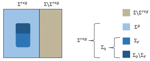
Figure 8. A schematic drawing which shows the relevant subsets of $\Sigma$. The shaded regions $\Sigma\backslash\Sigma^{reg}$ and $\Sigma_{0}\backslash\Sigma_{F}$ are subsets of $\Sigma$ which are of zero measure.

Appendix B Contracting an edge in a graph

As pointed out by Band and Lévy in [4, Appendix A], when the length of an edge tends to zero, the eigenvalues of the graph converge to the eigenvalues of the graph with this edge contracted. The edge to be contracted has Neumann conditions at its two end vertices and upon contraction, those vertices are merged, and the Neumann conditions are imposed on the newly formed vertex (see Figure 9). Here, we consider what happens when the torus variable corresponding to this edge is set to zero, which is needed for the proof of Theorem 4.3 given in Appendix C.

Lemma B.1.

Let $\Gamma$ be a magnetic standard graph. Let $e$ be an edge with no magnetic potential on it and with distinct endpoints both endowed with Neumann conditions. Let $\Gamma_{c}$ be the graph obtained from $\Gamma$ by contracting the edge $e$ and imposing Neumann condition at the newly formed vertex. Setting $\varkappa_{e}=0$ in the secular function of $\Gamma$ we obtain

(73) $$F((0,\vec{\varkappa}_{c});\vec{\alpha})=2\frac{d_{1}+d_{2}-2}{d_{1}d_{2}}F_{c}(\vec{\varkappa}_{c};\vec{\alpha}),$$

where $F_{c}$ is the secular function of $\Gamma_{c}$ , and $d_{1},d_{2}$ are the degrees of the endpoints of $e$.

Remark B.2.

If a graph $\Gamma$ has a loop and we set the corresponding variable to zero in the graph’s secular function, the secular function becomes identically zero. This is why we explicitly assumed in Lemma B.1 that the edge to be contracted has distinct endpoints.

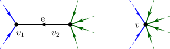
Figure 9. Contracting the edge $e$ in a graph. Here $d_{1}=3$ and $d_{2}=5$.

Proof.

[Proof of Lemma B.1] Assume we are contracting an edge connecting vertices $v_{1}$ and $v_{2}$ of degrees $d_{1}$ and $d_{2}$ correspondingly, see Figure 9. Let $e$ refer to the directed label of this edge going towards $v_{1}$ and $\hat{e}$ denote its reversal. Upon contraction of the edge $e$ the new joined vertex $v=v_{1}=v_{2}$ will have the degree $d_{1}+d_{2}-2$. The new graph will be denoted $\Gamma_{c}$ and its torus coordinates are $\vec{\varkappa}_{c}$.

Further assume that $e$ comes first in the numbering of edges (15) used in the set up of the secular equation (16). As a result, $\vec{\varkappa}=(\varkappa_{1},\vec{\varkappa}_{c})$. Once we set $\varkappa_{1}=0$, the matrix used in the definition of the secular function $F(\vec{\varkappa};\vec{\alpha})$ takes the form

(74) $$\boldsymbol{I}-e^{i(\vec{\varkappa}+\vec{\alpha})}\boldsymbol{S}=\left(\begin{array}[]{cc|c}1&1-\frac{2}{d_{2}}&-\frac{2}{d_{2}}\vec{r}_{2}\\ 1-\frac{2}{d_{1}}&1&-\frac{2}{d_{1}}\vec{r}_{1}\\ \hline\cr-\frac{2}{d_{1}}e^{i\xi}\vec{c}_{1}&-\frac{2}{d_{2}}e^{i\xi}\vec{c}_{2}&\boldsymbol{I}-e^{i\xi}\boldsymbol{S}_{r}\end{array}\right),$$

where $\xi=(\varkappa_{2}+\alpha_{2},\varkappa_{2}-\alpha_{2},\varkappa_{3}+\alpha_{3},\ldots)$ is the vector of torus coordinates and fluxes of all edges except the edge $e$ and $\boldsymbol{S}_{r}$ is the matrix $\boldsymbol{S}$ without its first two rows and columns. We have the relation $\vec{r}_{j}=(Jc_{j})^{T}$, where $J$ is a matrix which switches around the directed labels of the edges (see equation (43) and preceding discussion). Furthermore, the vectors $\vec{c}_{j}$ and $\vec{r}_{j}=(Jc_{j})^{T}$ contain zeros and ones only; for example, $\vec{r}_{2}$ has ones only in the entries corresponding to the edge labels coming into vertex $v_{2}$ while $\vec{c}_{1}$ has ones corresponding to edge labels coming out of $v_{1}$.

We would like to evaluate the determinant of (74) using Schur’s determinant identity in the form

(75) $$\det\begin{pmatrix}A&B\\ C&D\end{pmatrix}=\det(A)\det\left(D-CA^{-1}B\right).$$

We get

(76) $$F((0,\vec{\varkappa}_{c});\vec{\alpha})=2\frac{d_{1}+d_{2}-2}{d_{1}d_{2}}\det\left(\boldsymbol{I}-e^{i\xi}\boldsymbol{S}_{c}\right),$$

where the prefactor is the determinant of the top left corner and

$$\boldsymbol{S}_{c} =\boldsymbol{S}_{r}+\begin{pmatrix}\vec{c}_{1}&\vec{c}_{2}\end{pmatrix}\begin{pmatrix}\frac{2}{d_{1}}&0\\ 0&\frac{2}{d_{2}}\end{pmatrix}\begin{pmatrix}1&1-\frac{2}{d_{2}}\\ 1-\frac{2}{d_{1}}&1\end{pmatrix}^{-1}\begin{pmatrix}\frac{2}{d_{2}}&0\\ 0&\frac{2}{d_{1}}\end{pmatrix}\begin{pmatrix}\vec{r}_{2}\\ \vec{r}_{1}\end{pmatrix}$$

$$=\boldsymbol{S}_{r}+\begin{pmatrix}\vec{c}_{1}&\vec{c}_{2}\end{pmatrix}\begin{pmatrix}\frac{2}{d_{1}+d_{2}-2}&\frac{2}{d_{1}+d_{2}-2}-\frac{2}{d_{1}}\\ \frac{2}{d_{1}+d_{2}-2}-\frac{2}{d_{2}}&\frac{2}{d_{1}+d_{2}-2}\end{pmatrix}\begin{pmatrix}\vec{r}_{2}\\ \vec{r}_{1}\end{pmatrix}.$$

The effect of adding the term is best understood on some examples. If $e_{in}$ is one of the edges going to $v_{2}$ and $e_{out}$ is one of the edges coming out of $v_{1}$, then

$$(\boldsymbol{S}_{c})_{e_{out},e_{in}}=0+\begin{pmatrix}1&0\end{pmatrix}\begin{pmatrix}\frac{2}{d_{1}+d_{2}-2}&\frac{2}{d_{1}+d_{2}-2}-\frac{2}{d_{1}}\\ \frac{2}{d_{1}+d_{2}-2}-\frac{2}{d_{2}}&\frac{2}{d_{1}+d_{2}-2}\end{pmatrix}\begin{pmatrix}1\\ 0\end{pmatrix}=\frac{2}{d_{1}+d_{2}-2}.$$

If $e_{in}$ is one of the edges going to $v_{1}$ and $e_{out}$ is its reversal,

$$(\boldsymbol{S}_{c})_{e_{out},e_{in}}=\frac{2}{d_{1}}-1+\begin{pmatrix}1&0\end{pmatrix}\begin{pmatrix}\frac{2}{d_{1}+d_{2}-2}&\frac{2}{d_{1}+d_{2}-2}-\frac{2}{d_{1}}\\ \frac{2}{d_{1}+d_{2}-2}-\frac{2}{d_{2}}&\frac{2}{d_{1}+d_{2}-2}\end{pmatrix}\begin{pmatrix}0\\ 1\end{pmatrix}=\frac{2}{d_{1}+d_{2}-2}-1.$$

In both cases the answer is the correct scattering amplitude for the vertex $v$ of degree $d_{1}+d_{2}-2$ which resulted from the contraction of $e$ (see, for example, Figure 9, right). The remaining cases are checked analogously and we find that $\boldsymbol{S}_{c}$ is the bond scattering matrix of the graph $\Gamma_{c}$, so that

$$F_{c}(\vec{\varkappa}_{c};\vec{\alpha})=\det\left(\boldsymbol{I}-e^{i\xi}\boldsymbol{S}_{c}\right).$$

This, together with (76) gives (73).∎

We note that Lemma B.1 indeed implies the claim in [4, Appendix A], that graph eigenvalues are continuous with respect to edge length when the length goes to zero. Next, we provide another proof for this statement. The proof is insightful as it is done via the eigenfunctions. Yet, it does not reproduce the exact prefactor given in (73). More precisely, we now prove that

(77) $$F\left(0,\vec{\varkappa}_{c};\vec{\alpha}\right)=0\iff F_{c}\left(\vec{\varkappa}_{c};\vec{\alpha}\right)=0,$$

with notations similar to those in Lemma B.1.

First, we generalize the notion of canonical eigenfunction as given in Theorem 3.6(3). We do so by taking a canonical eigenfunction to be any eigenfunction belonging to the eigenvalue $k=1$ for a graph with edge lengths given by $\vec{l}=\vec{\varkappa}\in\Sigma$ (not just for $\vec{\varkappa}\in\Sigma^{reg}$ as in Theorem 3.6(3)). Now, the proof is based on showing a one to one correspondence between canonical eigenfunctions of $\Gamma$ with edge lengths $\vec{l}=\left(2\pi,\vec{\varkappa}_{c}\right)$ and canonical eigenfunctions of $\Gamma_{c}$ with edge lengths $\vec{l}_{c}=\vec{\varkappa}_{c}$. Let $f$ be a canonical eigenfunction of $\Gamma$ for edge lengths $\vec{l}=\left(2\pi,\vec{\varkappa}_{c}\right)$. Denote its restriction $\tilde{f}=f|_{\Gamma\setminus e_{0}}$ and consider $\tilde{f}$ to be a function on $\Gamma_{c}$ with $\vec{l}_{c}=\vec{\varkappa}_{c}$ under the identification of $v_{1}\sim v_{2}$. We will show that $\tilde{f}$ is actually a canonical eigenfunction of $\Gamma_{c}$. Note that we may write $f$ as

(78) $$f_{e}\left(t\right)=\begin{cases}\tilde{f}_{e}\left(t\right)&e\neq e_{0}\\ B\cos\left(t+\theta\right)&e=e_{0}\end{cases},$$

for some values of $B,\theta$. First of all, since $e_{0}$ is not a loop, $\tilde{f}$ cannot be identically zero. Otherwise the function $f$ would have zero value and zero derivative at $v_{1}$ and therefore would be identically zero on the edge $e_{0}$ as well. Denote the set of edge labels coming into $v_{i}$ and not including the labels $e_{0}$, $\hat{e}_{0}$ by $\mathcal{E}_{i}$ (blue and green edges in Figure 9). Let $e_{0}$ be oriented from $v_{2}$ to $v_{1}$ (see Figure 9). The Neumann conditions on the vertices imply that

$$\forall e\in\mathcal{E}_{1}\quad\quad f_{e}\left(l_{e}\right)=f_{e_{0}}\left(2\pi\right)=B\cos\left(\theta\right)$$

$$\forall e\in\mathcal{E}_{2}\quad\quad f_{e}\left(l_{e}\right)=f_{e_{0}}\left(0\right)=B\cos\left(\theta\right)$$

$$\sum_{e\in\mathcal{E}_{1}}\left(i\frac{d}{dx}+\frac{\alpha_{e}}{l_{e}}\right)f_{e}\left(l_{e}\right) =-i\frac{d}{dx}f_{e_{0}}\left(2\pi\right)=iB\sin\left(\theta\right)$$

$$\sum_{e\in\mathcal{E}_{2}}\left(i\frac{d}{dx}+\frac{\alpha_{e}}{l_{e}}\right)f_{e}\left(l_{e}\right) =i\frac{d}{dx}f_{e_{0}}\left(0\right)=-iB\sin\left(\theta\right),$$

where for convenience we have chosen the magnetic potential to be constant along each edge, $A_{e}\equiv\frac{\alpha_{e}}{l_{e}}$ (see (10)). It follows that

$$\forall e\in\left(\mathcal{E}_{1}\cup\mathcal{E}_{2}\right)\quad\quad f_{e}\left(l_{e}\right)=B\cos\left(\theta\right)$$

$$\sum_{e\in\left(\mathcal{E}_{1}\cup\mathcal{E}_{2}\right)}\left(i\frac{d}{dx}+\frac{\alpha_{e}}{l_{e}}\right)f_{e}\left(l_{e}\right) =0.$$

We get that if $f$ satisfies the Neumann boundary conditions at $v_{1}$ and $v_{2}$ then $\tilde{f}$ satisfies the Neumann boundary conditions at the merged vertex $v$. Obviously, $\tilde{f}$ satisfies the same vertex conditions as $f$ at all other vertices and it obeys $-\tilde{f}^{\prime\prime}=\tilde{f}$. Therefore $\tilde{f}$ is a canonical eigenfunction of $\Gamma_{c}$ with $\vec{l}=\vec{\varkappa}$.

In the other direction, assume that $\tilde{f}$ is a canonical eigenfunction of $\Gamma_{c}$ with edge lengths $\vec{l}_{c}=\vec{\varkappa}_{c}$. It can be extended to a canonical eigenfunction $f$ on $\Gamma$ with edge lengths $\vec{l}=\left(2\pi,\vec{\varkappa}_{c}\right)$, by setting $f$ to be as in (77), where $B,\theta$ are chosen to satisfy

$$B\cos\left(\theta\right) =\tilde{f}\left(v\right)$$

$$iB\sin\left(\theta\right) =\sum_{e\in\mathcal{E}_{1}}\left(i\frac{d}{dx}+\frac{\alpha_{e}}{l_{e}}\right)\tilde{f}|_{e}\left(l_{e}\right).$$

This proves (77). Furthermore, from the above also follows that the multiplicities of corresponding zeros of $F\left(0,\vec{\varkappa}_{c};\vec{\alpha}\right)$ and $F_{c}\left(\vec{\varkappa}_{c};\vec{\alpha}\right)=0$ are equal.

Appendix C Proof of Theorem 4.3

Proof of Theorem 4.3.

Let us have an in-depth look at the bond scattering matrix $\boldsymbol{S}$ of the graph $\Gamma$. We order the directed edge labels as follows: edge labels of $\Gamma_{1}$, edge labels of $\mathfrak{C}$ in the direction from $\Gamma_{1}$ to $\Gamma_{2}$, edge labels of $\mathfrak{C}$ in the opposite direction and then edge labels of $\Gamma_{2}$. With this order and edge groupings, the matrix $\boldsymbol{S}$ has the following block structure

(79) $$\boldsymbol{S}=\begin{pmatrix}\boldsymbol{S}_{1}&0&t_{1}&0\\ t_{1}^{\prime}&0&r_{1}&0\\ 0&r_{2}&0&t_{2}^{\prime}\\ 0&t_{2}&0&\boldsymbol{S}_{2}\end{pmatrix},$$

where, for example, the matrix $t_{1}$ corresponds to scattering of waves from $\mathfrak{C}$ into the subgraph $\Gamma_{1}$ and $r_{1}$ represents reflection of the waves from $\mathfrak{C}$, off $\Gamma_{1}$ and back into $\mathfrak{C}$. We have the relations $t_{i}^{\prime}=(J_{i}t_{i})^{T}$, where the permutation matrix $J_{i}$ switches the orientation of the edge labels in the subgraph $\Gamma_{i}$ (see equation (43) and preceding discussion).

We now multiply the matrix $\boldsymbol{S}$ by the diagonal matrix $e^{i\vec{\varkappa}+i\vec{\alpha}}$ which, in the block form similar to (79), is given by

(80) $$e^{i\vec{\varkappa}+i\vec{\alpha}}=\begin{pmatrix}e^{i\vec{\varkappa}_{1}+i\vec{\alpha}_{1}}&0&0&0\\ 0&e^{i\varkappa_{0}+i\vec{\alpha}_{0}}&0&0\\ 0&0&e^{i\varkappa_{0}-i\vec{\alpha}_{0}}&0\\ 0&0&0&e^{i\vec{\varkappa}_{2}+i\vec{\alpha}_{2}}\end{pmatrix}.$$

We would like to apply Schur’s determinant identity

(81) $$\det\begin{pmatrix}A&B\\ C&D\end{pmatrix}=\det(D)\det\left(A-BD^{-1}C\right),$$

to the determinant of the matrix $\boldsymbol{I}-e^{i\vec{\varkappa}+i\vec{\alpha}}\boldsymbol{S}$ written as

(82) $$\boldsymbol{I}-e^{i\vec{\varkappa}+i\vec{\alpha}}\boldsymbol{S}=\left(\begin{array}[]{ccc|c}\boldsymbol{I}_{1}-e^{i\vec{\varkappa}_{1}+i\vec{\alpha}_{1}}\boldsymbol{S}_{1}&0&-e^{i\vec{\varkappa}+i\vec{\alpha}_{1}}t_{1}&0\\ -e^{i\vec{\varkappa}_{0}+i\vec{\alpha}_{0}}t_{1}^{\prime}&\boldsymbol{I}_{0}&-e^{i\vec{\varkappa}_{0}+i\vec{\alpha}_{0}}r_{1}&0\\ 0&-e^{i\vec{\varkappa}_{0}-i\vec{\alpha}_{0}}r_{2}&\boldsymbol{I}_{0}&-e^{i\vec{\varkappa}_{0}-i\vec{\alpha}_{0}}t_{2}^{\prime}\\ \hline\cr 0&-e^{i\vec{\varkappa}_{2}+i\vec{\alpha}_{2}}t_{2}&0&\boldsymbol{I}_{2}-e^{i\vec{\varkappa}_{2}+i\vec{\alpha}_{2}}\boldsymbol{S}_{2}\end{array}\right).$$

The block $D$ is going to be $\boldsymbol{I}_{2}-e^{i\vec{\varkappa}_{2}+i\vec{\alpha}_{2}}\boldsymbol{S}_{2}$ and, as a first step, we would like to determine when it is invertible. Suppose, for a choice of $\vec{\varkappa}_{2}$ and $\vec{\alpha}_{2}$, the vector $\vec{v}_{2}$ is an eigenvector of $e^{i\vec{\varkappa}_{2}+i\vec{\alpha}_{2}}\boldsymbol{S}_{2}$ with eigenvalue $1$. Then the vector

(83) $$\vec{v}=(0,0,0,\vec{v}_{2}^{T})^{T}$$

is the eigenvector of $e^{i\vec{\varkappa}+i\vec{\alpha}}\boldsymbol{S}$ with eigenvalue $1$. Indeed, we know that the last entry $e^{i\vec{\varkappa}+i\vec{\alpha}}\boldsymbol{S}\vec{v}$ is going to be $\vec{v}_{2}$ and if any other entry is non-zero, it would mean that an application of $e^{i\vec{\varkappa}+i\vec{\alpha}}\boldsymbol{S}$ increases the norm of $\vec{v}$ which is impossible for a unitary matrix.

We conclude that $\boldsymbol{I}_{2}-e^{i\vec{\varkappa}_{2}+i\vec{\alpha}_{2}}\boldsymbol{S}_{2}$ is non-invertible only when the graph has an eigenfunction vanishing on the connector set $\mathfrak{C}$ and the entire subgraph $\Gamma_{1}$. When this is the case we have that (48) holds with $D_{2}=0$. To add on that, when this happens for $\vec{\alpha}=\vec{0}$, the eigenfunction mentioned above implies $\vec{\varkappa}\notin\Sigma^{g}$, which proves the claim at the end of the theorem.

Assuming the matrix is invertible, we have for $BD^{-1}C$

$$\begin{pmatrix}0\\ 0\\ -e^{i\varkappa_{0}-i\vec{\alpha}_{0}}t_{2}^{\prime}\end{pmatrix}\left(\boldsymbol{I}_{2}-e^{i\vec{\varkappa}_{2}+i\vec{\alpha}_{2}}\boldsymbol{S}_{2}\right)^{-1}\begin{pmatrix}0&-e^{i\vec{\varkappa}_{2}+i\vec{\alpha}_{2}}t_{2}&0\end{pmatrix}=\begin{pmatrix}0&0&0\\ 0&0&0\\ 0&e^{i\varkappa_{0}-i\vec{\alpha}_{0}}(Z_{2}-r_{2})&0\end{pmatrix},$$

where $Z_{2}$ is given

(84) $$Z_{2}(\vec{\varkappa}_{2};\vec{\alpha}_{2})=r_{2}+t_{2}^{\prime}\left(\boldsymbol{I}_{2}-e^{i\vec{\varkappa}_{2}+i\vec{\alpha}_{2}}\boldsymbol{S}_{2}\right)^{-1}e^{i\vec{\varkappa}_{2}+i\vec{\alpha}_{2}}t_{2},$$

which coincides with the definition of the scattering matrix of the subgraph $\Gamma_{2}$, see (45).

Subtracting this from the block $A$ we get

$$\det\left(\boldsymbol{I}-e^{i\vec{\varkappa}+i\vec{\alpha}}\boldsymbol{S}\right)=\det\left(\boldsymbol{I}_{2}-e^{i\vec{\varkappa}_{2}+i\vec{\alpha}_{2}}\boldsymbol{S}_{2}\right)\det\begin{pmatrix}\boldsymbol{I}_{1}-e^{i\vec{\varkappa}_{1}+i\vec{\alpha}_{1}}\boldsymbol{S}_{1}&0&-e^{i\vec{\varkappa}+i\vec{\alpha}_{1}}t_{1}\\ -e^{i\varkappa_{0}+i\vec{\alpha}_{0}}t_{1}^{\prime}&\boldsymbol{I}_{0}&-e^{i\vec{\varkappa}_{0}+i\vec{\alpha}_{0}}r_{1}\\ 0&-e^{i\vec{\varkappa}_{0}-i\vec{\alpha}_{0}}Z_{2}&\boldsymbol{I}_{0}\end{pmatrix}.$$

Applying Schur’s determinant identity again now with $\boldsymbol{I}_{1}-e^{i\vec{\varkappa}_{1}+i\vec{\alpha}_{1}}\boldsymbol{S}_{1}$ acting as a factor to bring outside, we get

$$\det\left(\begin{array}[]{c|cc}\boldsymbol{I}_{1}-e^{i\vec{\varkappa}_{1}+i\vec{\alpha}_{1}}\boldsymbol{S}_{1}&0&-e^{i\vec{\varkappa}+i\vec{\alpha}_{1}}t_{1}\\ \hline\cr-e^{i\varkappa_{0}+i\vec{\alpha}_{0}}t_{1}^{\prime}&\boldsymbol{I}_{0}&-e^{i\vec{\varkappa}_{0}+i\vec{\alpha}_{0}}r_{1}\\ 0&-e^{i\vec{\varkappa}_{0}-i\vec{\alpha}_{0}}Z_{2}&\boldsymbol{I}_{0}\end{array}\right)\\ =\det\left(\boldsymbol{I}_{1}-e^{i\vec{\varkappa}_{1}+i\vec{\alpha}_{1}}\boldsymbol{S}_{1}\right)\det\begin{pmatrix}\boldsymbol{I}_{0}&-e^{i\vec{\varkappa}_{0}+i\vec{\alpha}_{0}}Z_{1}\\ -e^{i\vec{\varkappa}_{0}-i\vec{\alpha}_{0}}Z_{2}&\boldsymbol{I}_{0}\end{pmatrix},$$

where in the above we used an expression of $Z_{1}$ similar to (84) and also assumed the invertibility of $\boldsymbol{I}_{1}-e^{i\vec{\varkappa}_{1}+i\vec{\alpha}_{1}}\boldsymbol{S}_{1}$. If it is not invertible, we get just as before that $D_{1}=0$ and (48) still holds. Evaluating the last determinant (using Schur’s identity once more), we get

$$\det\begin{pmatrix}\boldsymbol{I}_{0}&-e^{i\vec{\varkappa}_{0}+i\vec{\alpha}_{0}}Z_{1}\\ -e^{i\vec{\varkappa}_{0}-i\vec{\alpha}_{0}}Z_{2}&\boldsymbol{I}_{0}\end{pmatrix}=\det(\boldsymbol{I}_{0})\det\left(\boldsymbol{I}_{0}-e^{i\vec{\varkappa}_{0}+i\vec{\alpha}_{0}}Z_{1}e^{i\vec{\varkappa}_{0}-i\vec{\alpha}_{0}}Z_{2}\right).$$

If all entries of $\vec{\varkappa}_{0}$ are different than zero, collecting all the factors above together gives (48) with the prefactor $c=1$ at its right hand side. Otherwise, for any vanishing entry of $\vec{\varkappa}_{0}$, we apply Lemma B.1 to conclude that (48) still holds. This time, the prefactor $c$ in (48) equals the product of prefactors at the right hand side of (73), applied for each of the vanishing entries in $\vec{\varkappa}_{0}$. ∎

Appendix D Examples of nodal surplus distribution

In this appendix we will calculate, analytically or numerically, the nodal surplus distribution of the graphs shown in the Figure 10. We say that a graph is a $[p_{1},p_{2},\ldots,p_{n}]$ chain if the graph consists of a sequence of $n+1$ vertices with $p_{k}$ edges connecting vertices $v_{k}$ and $v_{k+1}$. Note that the graphs we call “figure of 8” (Figure 10(a)) and “dumbbell” (Figure 10(b)) can be considered as a $[2,2]$ chain and a $[2,1,2]$ chain correspondingly. This terminology for “chains” comes from the notion of “mandarin chain” or “pumpkin chain” graphs which appeared in [38, 4].

Figure 10. Graphs considered in Section D: (a) “figure of 8”, (b) “dumbbell”, (c) “$[1,2,2,1]$ chain”, (d) “$[3,2,1]$ chain”.

The results are summarized in Table 1. Example (b) satisfies the assumptions of Theorem 2.3 and therefore has a binomial distribution, which we confirm both analytically and numerically. Examples (a), (d) show that these assumptions are essential as there are graphs with non-binomial distribution. Example (c) shows that not all graphs with binomial distribution can be characterized as edge-separated, so the interesting question of characterizing all the graphs with binomial distributions remains open.

	Edge-separated	Not edge-separated
Binomial distribution	(b) “dumbbell”	(c) “$[1,2,2,1]$ chain”
Non-binomial distribution		(a) “figure of 8”, (d) “$[3,2,1]$ chain”

Table 1. A summary of the results of Section D.

D.1. A figure of 8 graph

Consider the graph shown in Figure 10(a) (A figure of 8 graph). The torus which describes this graph is $\mathbb{T}^{2}=\mathbb{R}^{2}/(2\pi\mathbb{Z})^{2}$. Using the coordinates $\left(x_{1},x_{2}\right)\in\mathbb{T}^{2}$, the real secular function (28) can be calculated to be

(85) $$F_{R}\left(x_{1},x_{2};\alpha_{1},\alpha_{2}\right)=2\left(\cos\alpha_{2}\sin x_{1}+\cos\alpha_{1}\sin x_{2}-\sin\left(x_{1}+x_{2}\right)\right).$$

For $\vec{\alpha}=0$ we get a nice form of

$$F_{R}\left(x_{1},x_{2};0,0\right) =8\sin\left(\frac{x_{1}}{2}\right)\sin\left(\frac{x_{2}}{2}\right)\sin\left(\frac{x_{1}+x_{2}}{2}\right).$$

It is not hard to show that (see also Figure 11),

$$\Sigma^{reg} =\left\{\left(x_{1},x_{2}\right)\in\mathbb{T}^{2}~{}:~{}\,x_{1}=0~{}\textrm{or}~{}x_{2}=0~{}\textrm{or}~{}x_{1}+x_{2}\equiv 0\thinspace\thinspace(\textrm{mod }2\pi)\right\}\backslash\left\{\left(0,0\right)\right\}$$

$$\Sigma_{0}=\Sigma_{F} =\left\{\left(\pi,\pi\right)\right\}\cup\left\{\left(x_{1},x_{2}\right)\in\mathbb{T}^{2}~{}:~{}\,x_{1}=0~{}\textrm{or}~{}x_{2}=0\right\}\backslash\left\{\left(0,0\right)\right\}$$

$$\Sigma^{g}=\Sigma^{reg}\backslash\Sigma_{0}=\left\{\left(x_{1},x_{2}\right)\in\mathbb{T}^{2}~{}:~{}\,x_{1}+x_{2}\equiv 0\thinspace\thinspace(\textrm{mod }2\pi)\right\}\backslash\left\{\left(0,0\right),\thinspace\left(\pi,\pi\right)\right\}.$$

Note that $\Sigma_{0}$ is defined in (30) as a subset of $\Sigma^{reg}$ for which the corresponding eigenfunctions vanish at some vertex. Also, $\Sigma_{F}$ is defined in (72) as a subset of $\Sigma{0}$, for which the corresponding eigenfunctions are supported on a loop. See also Figure 8 which shows this decomposition of the secular manifold.

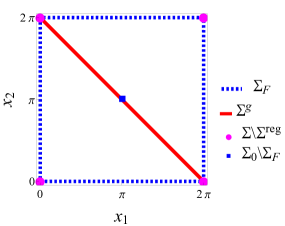
(a)   (b)

Figure 11. (a) The secular manifold of the “figure of 8” graph with different subsets ($\Sigma^{reg}$, $\Sigma_{0}$, $\Sigma_{F}$ and $\Sigma^{g}$) highlighted by different colors. (b) The “figure of 8” graph.

In addition, a straightforward calculation shows that for $\vec{\varkappa}\in\Sigma^{g}$ (for which $\sin\left(\frac{x_{1}+x_{2}}{2}\right)=0$) we get

$$\nabla_{x}F_{R}\cdot\vec{l}=4\sin\left(\frac{x_{1}}{2}\right)\sin\left(\frac{x_{2}}{2}\right)\cos\left(\frac{x_{1}+x_{2}}{2}\right)\left(l_{1}+l_{2}\right)=-4\sin\left(\frac{x_{1}}{2}\right)\sin\left(\frac{x_{2}}{2}\right)\left(l_{1}+l_{2}\right)<0.$$

Thus

(86) $$-\frac{H_{\alpha}F_{R}}{\nabla_{x}F_{R}\cdot\vec{l}} =-\frac{1}{4\sin\left(\frac{x_{1}}{2}\right)\sin\left(\frac{x_{2}}{2}\right)\left(l_{1}+l_{2}\right)}\begin{pmatrix}2\sin\left(x_{2}\right)&0\\ 0&2\sin\left(x_{1}\right)\end{pmatrix},$$

(87) $$\sigma\left(\vec{\varkappa}\right) =\mathcal{M}\left(-\frac{H_{\alpha}F_{R}}{\nabla_{x}F_{R}\cdot\vec{l}}\right)=\mathcal{M}\begin{pmatrix}-\sin\left(x_{2}\right)&0\\ 0&-\sin\left(x_{1}\right)\end{pmatrix}$$

and as for $\vec{\varkappa}\in\Sigma^{g}$ we have $x_{1}+x_{2}=2\pi$, this gives

(88) $$\sigma\left(\vec{\varkappa}\right)=\mathcal{M}\begin{pmatrix}\sin\left(x_{1}\right)&0\\ 0&-\sin\left(x_{1}\right)\end{pmatrix}\equiv 1,$$

with the following local surplus functions

$$\forall\vec{\varkappa}\in\Sigma^{g}\,\,,\sigma^{\left(i\right)}\left(x_{i}\right) =\begin{cases}0&x_{i}\in\left(0,\pi\right)\\ 1&x_{i}\in\left(\pi,2\pi\right)\end{cases}.$$

It is obvious from (88) that the surplus distribution is not binomial. In addition, this example nicely demonstrates that local surpluses may be anti correlated, $\mathbb{P}\left(\sigma^{(1)}=j\left|\sigma^{(2)}=j\right.\right)=0$.

Remark D.1.

Another approach in this simple case, would be to notice that for a given choice of rationally independent lengths $\vec{l}$, we have two kinds of eigenfunctions. The first kind are the eigenfunctions supported on one of the loops and zero on the other, with corresponding eigenvalues in $k\in\frac{2\pi}{l_{1}}\mathbb{Z}\cup\frac{2\pi}{l_{2}}\mathbb{Z}$. The second kind of eigenfunctions can be obtained from an eigenfunction of a circle of length $l_{1}+l_{2}$, under identification of two points with the same function value which are at $l_{1}$ distance apart. Such eigenfunctions, which are generic, would correspond to eigenvalues $k\in\frac{2\pi}{l_{1}+l_{2}}\mathbb{Z}$ and their nodal count will therefore be $\phi=\frac{k\left(l_{1}+l_{2}\right)}{\pi}$. It remains to figure the position in the spectrum of such an eigenvalue. One can check that the two sets $A=\frac{2\pi}{l_{1}}\mathbb{Z}\cup\frac{2\pi}{l_{2}}\mathbb{Z}$ and $B=\frac{2\pi}{l_{1}+l_{2}}\mathbb{Z}$ interlace and as the second eigenvalue after $k_{1}=0$ will be $k_{2}=\frac{2\pi}{l_{1}+l_{2}}$, then we get that the generic eigenvalues will be the even ones $k_{2n}=n\frac{2\pi}{l_{1}+l_{2}}$ with

$$\phi_{2n}=\frac{k_{2n}\left(l_{1}+l_{2}\right)}{\pi}=2n~{}~{}\Rightarrow~{}~{}\sigma\equiv 1$$

D.2. A dumbbell graph

Consider the graph shown in Figure 12(b) (“dumbbell” graph).

Its real secular function (28) can be calculated to be

(89) $$F_{R}\left(x_{1},x_{2},x_{3};\alpha_{1},\alpha_{2}\right)=\frac{16}{9}\cos x_{2}\Big{(}\cos\alpha_{1}\sin x_{3}+\cos\alpha_{2}\sin x_{1}-\sin\left(x_{1}+x_{3}\right)\Big{)}\\ -\frac{8}{9}\sin x_{2}\Big{(}4\left(\cos\alpha_{1}-\cos x_{1}\right)\left(\cos\alpha_{2}-\cos x_{3}\right)-\sin x_{1}\sin x_{3}\Big{)}.$$

Observe that by taking the limit $x_{2}\rightarrow 0$ we recover the secular function of the figure of 8 graph, (85), up to a factor of $\frac{8}{9}$, which demonstrates the result of Lemma B.1.

For $\vec{\alpha}=0$ we get for the secular function

(90) $$F_{R}\left(x_{1},x_{2},x_{3};0,0\right)=\frac{16}{9}\sin\frac{x_{1}}{2}\sin\frac{x_{3}}{2}\left(-\sin x_{2}\left(3\cos\frac{x_{1}-x_{3}}{2}-5\cos\frac{x_{1}+x_{3}}{2}\right)\right.\\ \left.+4\cos x_{2}\sin\frac{x_{1}+x_{3}}{2}\right)$$

and correspondingly the Hessian is

(91) $$H_{\alpha}F_{R}\left(x_{1},x_{2},x_{3};0,0\right)\\ =\frac{8}{9}\begin{pmatrix}4\sin x_{2}\left(1-\cos x_{3}\right)-2\cos x_{2}\sin x_{3}&0\\ 0&4\sin x_{2}\left(1-\cos x_{1}\right)-2\cos x_{2}\sin x_{1}\end{pmatrix}.$$

We may use (90) in order to extract $x_{2}\left(x_{1},x_{3}\right)$ for points $\vec{\varkappa}\in\Sigma^{g}$ and thus get the following expressions in terms of $x_{1},x_{3}$ solely,

$$-\frac{H_{\alpha}\left(F\right)}{\nabla F_{R}\cdot\vec{l}}=\frac{\begin{pmatrix}4\sin\frac{x_{3}}{2}\cos\frac{x_{1}}{2}C(x_{3})&0\\ 0&4\sin\frac{x_{1}}{2}\cos\frac{x_{3}}{2}C(x_{1})\end{pmatrix}}{2\sin\frac{x_{1}}{2}\sin\frac{x_{3}}{2}\left(2C(x_{3})l_{1}+C(x_{3})C(x_{1})l_{2}+2C(x_{1})l_{3}\right)},\\$$

where $C(x)=5-3\cos x$ is never zero. Therefore,

$$\sigma\left(\vec{\varkappa}\right)=\mathcal{M}\left(-\frac{H_{\alpha}\left(F\right)}{\nabla F_{R}\cdot\vec{l}}\right)=\mathcal{M}\begin{pmatrix}\cot\frac{x_{1}}{2}&0\\ 0&\cot\frac{x_{3}}{2}\end{pmatrix}.$$

By the above, the local surplus functions are given by

$$\sigma^{\left(1\right)}\left(x_{1}\right)=\begin{cases}0&x_{1}\in\left(0,\pi\right)\\ 1&x_{1}\in\left(\pi,2\pi\right)\end{cases}, \quad\quad\sigma^{\left(2\right)}\left(x_{3}\right)=\begin{cases}0&x_{3}\in\left(0,\pi\right)\\ 1&x_{3}\in\left(\pi,2\pi\right)\end{cases}.$$

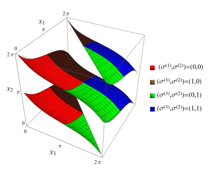
(a) (b)

Figure 12. The generic secular manifold $\Sigma^{g}$ for the “dumbbell graph”. It is depicted in four colors, according to all possible values for the local surpluses. (b) The “dumbbell” graph with torus coordinates and magnetic fluxes marked on corresponding edges.

Figure 12(a) shows the secular manifold of the “dumbbell” graph with different local nodal surpluses indicated by color. In Figure 13, we give a normalized histogram of the nodal surplus for the first $10^{6}$ eigenfunctions calculated numerically for the rationally independent lengths $\vec{l}=\left(\pi,e,1\right)$. We compare it in the figure to the binomial distribution $\operatorname{Bin}\left(2,\frac{1}{2}\right)$ and find a perfect match according to the prediction of Theorem 2.3.

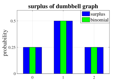
Figure 13. The normalized histogram of the nodal surplus of the “dumbbell” graph calculated from the first $10^{6}$ eigenfunctions, compared to the relevant binomial distribution.

D.3. A $[1,2,2,1]$ pumpkin chain

Consider the $[1,2,2,1]$ chain graph shown in Figure 14(b). In Figure 14(a), we give a normalized histogram of the nodal surplus for the first $10^{6}$ eigenfunctions calculated numerically for the rationally independent lengths

$$\vec{l}=\left(\pi,e,1,\sqrt{2},\sqrt{3},\sqrt{5}\right).$$

We compare it in the figure to the binomial distribution $\operatorname{Bin}\left(2,\frac{1}{2}\right)$ and find that they match. This is in spite of the fact that this graph does not satisfy the assumptions of Theorem 2.3, as its cycles are not edge-separated. This numerical finding calls for a further investigation.

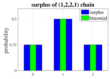
(a)   (b)

Figure 14. (a) The normalized histogram of the nodal surplus of the $[1,2,2,1]$ pumpkin chain calculated from the first $10^{6}$ eigenfunctions, compared to the relevant binomial distribution. (b) The $[1,2,2,1]$ pumpkin chain graph.

D.4. A $[3,2,1]$ pumpkin chain

Consider the $[3,2,1]$ chain graph shown in Figure 15(b). In Figure 15(a), we show a normalized histogram of the nodal surplus for the first $10^{6}$ eigenfunctions calculated numerically for the rationally independent lengths $\vec{l}=\left(\pi,e,1,\sqrt{2},\sqrt{3},\sqrt{5}\right)$. We compare it in the figure to the binomial distribution $\operatorname{Bin}\left(3,\frac{1}{2}\right)$ as $\beta=3$ for this graph.

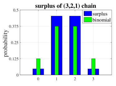
(a)   (b)

Figure 15. (a) The normalized histogram of the nodal surplus of the $[3,2,1]$ chain graph calculated from the first $10^{6}$ eigenfunctions, compared to the relevant binomial distribution. (b) The $[3,2,1]$ chain graph.

It is easy to notice that there is no match and the nodal surplus probability of the $\left(3,2,1\right)$ chain graph is not binomial. We further investigate this graph by examining the conditional probabilities of its local surpluses. Note that this graph has two vertex-separated blocks, of Betti numbers, $\beta^{(1)}=2,~{}\beta^{(2)}=1$. First, we calculate numerically the conditional probability, $\mathbb{P}\left(\sigma^{(2)}=s\left|\sigma^{(1)}\right.\right)$ for different values of $\sigma^{(1)}$ and see that it is not symmetric (shown in Figure 16(a)). Then, we do the same for the other conditional probability, $\mathbb{P}\left(\sigma^{(1)}=s\left|\sigma^{(2)}\right.\right)$ in Figure 16(b)) and once again find no symmetry. This demonstrates that the property of independently symmetric local surpluses (see Theorem 4.18) does not hold for this graph.

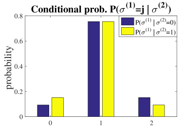
(a) (b)

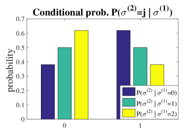
Figure 16. The normalized histograms of the conditional probability of local surpluses for the graph in Figure 10(d) calculated from the first $10^{6}$ eigenfunctions. (a) $\mathbb{P}\left(\sigma^{(1)}=j\left|\sigma^{(2)}\right.\right)$, (b) $\mathbb{P}\left(\sigma^{(2)}=j\left|\sigma^{(1)}\right.\right)$

References

- [1] R. Band. The nodal count implies the graph is a tree. Philos. Trans. R. Soc. Lond. A, 372(2007):20120504, 24, 2014. preprint arXiv:1212.6710.
- [2] R. Band and G. Berkolaiko. Universality of the momentum band density of periodic networks. Phys. Rev. Lett., 111:130404, Sep 2013.
- [3] R. Band, G. Berkolaiko, and U. Smilansky. Dynamics of nodal points and the nodal count on a family of quantum graphs. Annales Henri Poincare, 13(1):145–184, 2012.
- [4] R. Band and G. Lévy. Quantum graphs which optimize the spectral gap. preprint arXiv:1608.00520, 2016.
- [5] R. Band, I. Oren, and U. Smilansky. Nodal domains on graphs—how to count them and why? In Analysis on graphs and its applications, volume 77 of Proc. Sympos. Pure Math., pages 5–27. Amer. Math. Soc., Providence, RI, 2008.
- [6] R. Band, T. Shapira, and U. Smilansky. Nodal domains on isospectral quantum graphs: the resolution of isospectrality? J. Phys. A, 39(45):13999–14014, 2006.
- [7] F. Barra and P. Gaspard. On the level spacing distribution in quantum graphs. J. Statist. Phys., 101(1–2):283–319, 2000.
- [8] D. Beliaev and Z. Kereta. On the Bogomolny-Schmit conjecture. J. Phys. A, 46(45):455003, 5, 2013.
- [9] G. Berkolaiko. A lower bound for nodal count on discrete and metric graphs. Comm. Math. Phys., 278(3):803–819, 2008.
- [10] G. Berkolaiko. Nodal count of graph eigenfunctions via magnetic perturbation. Anal. PDE, 6:1213–1233, 2013. preprint arXiv:1110.5373.
- [11] G. Berkolaiko. Elementary introduction to quantum graphs. preprint arXiv:1603.07356 [math-ph], 2016.
- [12] G. Berkolaiko and P. Kuchment. Introduction to Quantum Graphs, volume 186 of Mathematical Surveys and Monographs. AMS, 2013.
- [13] G. Berkolaiko, Yu. Latushkin, and S. Sukhtaiev. On limits of quantum graph operators with shrinking edges. in preparation, 2017.
- [14] G. Berkolaiko and W. Liu. Simplicity of eigenvalues and non-vanishing of eigenfunctions of a quantum graph. J. Math. Anal. Appl., 445(1):803–818, 2017. preprint arXiv:1601.06225.
- [15] G. Berkolaiko and T. Weyand. Stability of eigenvalues of quantum graphs with respect to magnetic perturbation and the nodal count of the eigenfunctions. Philos. Trans. R. Soc. Lond. Ser. A Math. Phys. Eng. Sci., 372(2007):20120522, 17, 2014.
- [16] G. Berkolaiko and B. Winn. Relationship between scattering matrix and spectrum of quantum graphs. Trans. Amer. Math. Soc., 362(12):6261–6277, 2010.
- [17] G. Blum, S. Gnutzmann, and U. Smilansky. Nodal domains statistics: A criterion for quantum chaos. Phys. Rev. Lett., 88(11):114101, 2002.
- [18] E. Bogomolny and C. Schmit. Percolation model for nodal domains of chaotic wave functions. Phys. Rev. Lett., 88:114102, Mar 2002.
- [19] Y. Colin de Verdière. Magnetic interpretation of the nodal defect on graphs. Anal. PDE, 6:1235–1242, 2013. preprint arXiv:1201.1110.
- [20] Y. Colin de Verdière. Semi-classical measures on quantum graphs and the Gauß map of the determinant manifold. Annales Henri Poincaré, 16(2):347–364, 2015. also arXiv:1311.5449.
- [21] Y. Colin de Verdière and F. Truc. Topological resonances on quantum graphs. preprint arXiv:1604.01732, 2016.
- [22] R. Courant. Ein allgemeiner Satz zur Theorie der Eigenfunktione selbstadjungierter Differentialausdrücke. Nach. Ges. Wiss. Göttingen Math.-Phys. Kl., pages 81–84, July 1923.
- [23] E. B. Davies, P. Exner, and J. Lipovský. Non-Weyl asymptotics for quantum graphs with general coupling conditions. J. Phys. A, 43(47):474013, 16, 2010.
- [24] E.B. Davies and A. Pushnitski. Non-Weyl resonance asymptotics for quantum graphs. Analysis & PDE, 4:729–756, 2011.
- [25] Reinhard Diestel. Graph theory, volume 173 of Graduate Texts in Mathematics. Springer, Heidelberg, fourth edition, 2010.
- [26] P. Exner and O. Turek. Periodic quantum graphs from the Bethe–Sommerfeld perspective. preprint arXiv:1705.07306, 2017.
- [27] L. Friedlander. Genericity of simple eigenvalues for a metric graph. Israel J. Math., 146:149–156, 2005.
- [28] S. A. Fulling, P. Kuchment, and J. H. Wilson. Index theorems for quantum graphs. J. Phys. A, 40(47):14165–14180, 2007.
- [29] N. I. Gerasimenko and B. S. Pavlov. A scattering problem on noncompact graphs. Teoret. Mat. Fiz., 74(3):345–359, 1988.
- [30] A. Ghosh, A. Reznikov, and P. Sarnak. Nodal domains of Maass forms I. Geom. Funct. Anal., 23(5):1515–1568, 2013.
- [31] S. Gnutzmann, P. D. Karageorge, and U. Smilansky. Can one count the shape of a drum? Phys. Rev. Lett., 97(9):090201, 4, 2006.
- [32] S. Gnutzmann and U. Smilansky. Quantum graphs: Applications to quantum chaos and universal spectral statistics. Adv. Phys., 55(5–6):527–625, 2006.
- [33] S. Gnutzmann, U. Smilansky, and N. Sondergaard. Resolving isospectral ‘drums’ by counting nodal domains. J. Phys. A, 38(41):8921–8933, 2005.
- [34] S. Gnutzmann, U. Smilansky, and J. Weber. Nodal counting on quantum graphs. Waves Random Media, 14(1):S61–S73, 2004.
- [35] J. Jung and S. Zelditch. Number of nodal domains and singular points of eigenfunctions of negatively curved surfaces with an isometric involution. J. Differential Geom., 102(1):37–66, 2016.
- [36] J. Jung and S. Zelditch. Number of nodal domains of eigenfunctions on non-positively curved surfaces with concave boundary. Math. Ann., 364(3-4):813–840, 2016.
- [37] P. D. Karageorge and U. Smilansky. Counting nodal domains on surfaces of revolution. J. Phys. A, 41(20):205102, 2008.
- [38] J. B. Kennedy, P. Kurasov, G. Malenová, and D. Mugnolo. On the spectral gap of a quantum graph. Ann. Henri Poincaré, 17(9):2439–2473, 2016.
- [39] K. Konrad. Asymptotic statistics of nodal domains of quantum chaotic billiards in the semiclassical limit. Senior Thesis Dartmouth College, 2012.
- [40] V. Kostrykin and R. Schrader. Kirchhoff’s rule for quantum wires. J. Phys. A, 32(4):595–630, 1999.
- [41] V. Kostrykin and R. Schrader. The generalized star product and the factorization of scattering matrices on graphs. J. Math. Phys., 42(4):1563–1598, 2001.
- [42] V. Kostrykin and R. Schrader. Quantum wires with magnetic fluxes. Comm. Math. Phys., 237(1-2):161–179, 2003. Dedicated to Rudolf Haag.
- [43] T. Kottos and U. Smilansky. Quantum chaos on graphs. Phys. Rev. Lett., 79(24):4794–4797, 1997.
- [44] T. Kottos and U. Smilansky. Periodic orbit theory and spectral statistics for quantum graphs. Ann. Physics, 274(1):76–124, 1999.
- [45] T. Kottos and U. Smilansky. Chaotic scattering on graphs. Phys. Rev. Lett., 85(5):968–971, 2000.
- [46] D. Mugnolo. Semigroup methods for evolution equations on networks. Understanding Complex Systems. Springer, Cham, 2014.
- [47] M. Nastasescu. The number of ovals of a random real plane curve. Senior Thesis Princeton University, 2011.
- [48] F. Nazarov and M. Sodin. On the number of nodal domains of random spherical harmonics. Amer. J. Math., 131(5):1337–1357, 2009.
- [49] Åke Pleijel. Remarks on Courant’s nodal line theorem. Comm. Pure Appl. Math., 9:543–550, 1956.
- [50] Yu. V. Pokornyĭ, V. L. Pryadiev, and A. Al′-Obeĭd. On the oscillation of the spectrum of a boundary value problem on a graph. Mat. Zametki, 60(3):468–470, 1996.
- [51] C. Rouvinez and U. Smilansky. A scattering approach to the quantization of Hamiltonians in two dimensions—application to the wedge billiard. J. Phys. A, 28(1):77–104, 1995.
- [52] H. Schanz and U. Smilansky. Quantization of Sinai’s billiard—a scattering approach. Chaos Solitons Fractals, 5(7):1289–1309, 1995.
- [53] P. Schapotschnikow. Eigenvalue and nodal properties on quantum graph trees. Waves Random Complex Media, 16(3):167–178, 2006.
- [54] G. Shmuel and R. Band. Universality of the frequency spectrum of laminates. Journal of the Mechanics and Physics of Solids, 92:127 – 136, 2016.
- [55] Uzy Smilansky. Exterior-interior duality for discrete graphs. J. Phys. A, 42(3):035101, 13, 2009.
- [56] C Sturm. Mémoire sur les équations différentielles linéaires du second ordre. J. Math. Pures Appl., 1:106–186, 1836.
- [57] W. T. Tutte. Graph theory, volume 21 of Encyclopedia of Mathematics and its Applications. Addison-Wesley Publishing Company, Advanced Book Program, Reading, MA, 1984.
- [58] J. von Below. A characteristic equation associated to an eigenvalue problem on -networks. Linear Algebra Appl., 71:309–325, 1985.
- [59] H. Weyl. Über die Gleichverteilung von Zahlen mod. Eins. Math. Ann., 77(3):313–352, 1916.