“Haldane” phases with ultracold fermionic atoms in double-well optical lattices

Abstract

We propose to realize one-dimensional topological phases protected by SU($N$) symmetry using alkali or alkaline-earth atoms loaded into a bichromatic optical lattice. We derive a realistic model for this system and investigate it theoretically. Depending on the parity of $N$, two different classes of symmetry-protected topological (SPT) phases are stabilized at half-filling for physical parameters of the model. For even $N$, the celebrated spin-1 Haldane phase and its generalization to SU($N$) are obtained with no local symmetry breaking. In stark contrast, at least for $N=3$, a new class of SPT phases, dubbed chiral Haldane phases, that spontaneously break inversion symmetry, emerge with a two-fold ground-state degeneracy. The latter ground states with open-boundary conditions are characterized by different left and right boundary spins which are related by conjugation. Our results show that topological phases are within close reach of the latest experiments on cold fermions in optical lattices.

Introduction – Symmetry protected topological (SPT) phases have attracted a lot of attention over recent years. These new quantum phases exhibit short-range entanglement and possess only conventional gapped excitations in the bulk, while hosting non-trivial symmetry-protected surface states wenbook ; senthilreview . A paradigmatic example of one-dimensional (1D) bosonic SPT phases is the Haldane phase found in the spin-1 antiferromagnetic spin chain haldane . In the bulk, the phase looks ordinary, but, in the case of an open-boundary condition Kennedy-90 or when the chain is cut by doping impurities hagiwara , non-trivial spin-1/2 edge states appear. This phase is protected by the SO(3) symmetry underlying the Heisenberg model, and more generally, by at least one of the three discrete symmetries: the dihedral group of $\pi$-rotations along the $x,y,z$ axes, time-reversal or inversion symmetries gu ; pollmann .

A fairly complete understanding of 1D bosonic SPT phases has been obtained through various approaches such as group cohomology, matrix-product states, entanglement spectroscopy, and field-theoretical arguments chenx ; schuch ; fidowski ; Pollmann2010 ; xu . The possible 1D SPT phases associated with a given protecting symmetry $G$ are classified by its projective representations, i.e., the second cohomology group ${\cal H}^{2}(G,\text{U(1)})$. For instance, in the presence of SO(3) symmetry, there is a $\mathbb{Z}_{2}$ classification and the Haldane phase is the only SPT phase whose edge states obey a non-trivial projective representation gu ; pollmann .

Richer SPT phases can be obtained when $G$ is a more general Lie group. For instance, the group SU($N$) leads to a $\mathbb{Z}_{N}$ classification predicting $N-1$ non-trivial SPT phases Duivenvoorden-Q-13 protected by SU($N$) (PSU($N$), more precisely comment ) or by its discrete subgroup $\mathbb{Z}_{N}$ $\times$ $\mathbb{Z}_{N}$ Else-B-D-13 ; Duivenvoorden-Q-ZnxZn-13 . The edge states of these SPT phases are labeled by the inequivalent projective representations of SU($N$) which are specified by $\mathbb{Z}_{N}$ quantum numbers $n_{\rm top}=n_{\text{Y}}({\rm mod}\;N)$, with $n_{\text{Y}}$ being the number of boxes in the Young diagram corresponding to the representation of the boundary spins Duivenvoorden-Q-13 ; Capponi-L-T-15 . In stark contrast to the $N=2$ case, i.e. $G=\text{SO(3)}$, where all the projective representations are self-conjugate, the left and right edge states of the SU($N$) SPT phases with $N>2$ might belong to different projective representations that are related by conjugation. This leads to an interesting class of SPT phases, dubbed chiral Haldane ($\chi$H), which spontaneously break the inversion symmetry. These phases are partially characterized by local order parameters and exist in pairs; in one phase, the left and right edge states transform respectively in the SU($N$) representation $\mathcal{R}$ and its conjugate $\bar{\mathcal{R}}$, and vice-versa in the other Furusaki2014 ; greiter ; AKLT ; Quella2015 . In the following, we label the SPT phases by the number of boxes in the Young diagrams as $(n_{\text{Y}}(\mathcal{R}),n_{\text{Y}}(\bar{\mathcal{R}}))$ (mod $N$). In reflection-symmetric systems, the two topological ground states $(n_{\text{Y}}(\mathcal{R}),n_{\text{Y}}(\bar{\mathcal{R}}))$ and $(n_{\text{Y}}(\bar{\mathcal{R}}),n_{\text{Y}}(\mathcal{R}))$ are degenerate.

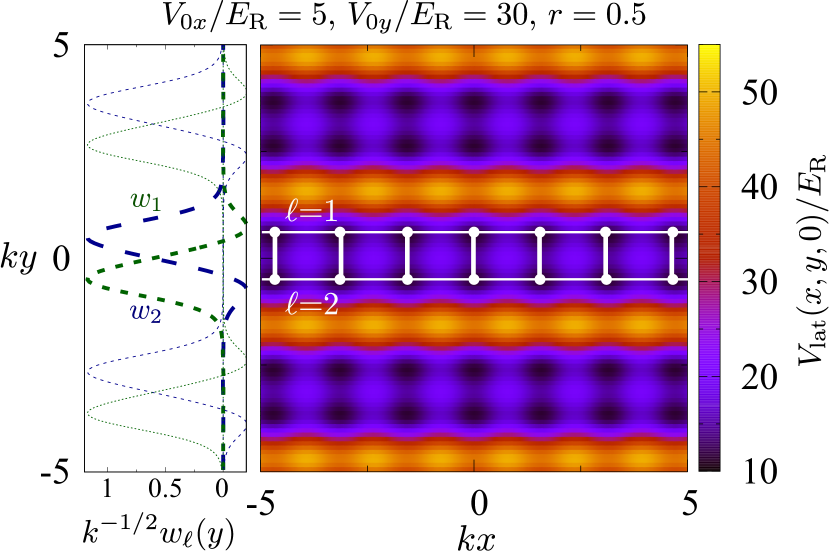
Figure 1: (Color online) The potential $V_{\mathrm{lat}}$ in the $xy$ plane (right panel): three double-well ladder systems are visible. The two independent Wannier functions $w_{1}(y)$ and $w_{2}(y)$ along $y$ (left, green and blue) are centered on the two chains ($\ell=1,2$). Lengths and energies are respectively expressed in units of the reduced wavelength $1/k$ and the recoil energy $E_{R}=\hbar^{2}k^{2}/2m$. This optical potential yields $t_{\perp}/t=2.9$ and $V/U=0.086$.

In this Letter, we propose an implementation of the Haldane phase ($N=2$) and its generalizations to even-$N$, as well as the $\chi$H phases for $N=3$, with half-filled ultracold fermions loaded into 1D double-well optical lattices. Thanks to their cleanness and controllability, these systems offer an ideal framework for the realization of the SPT phases, which requires precise symmetries. The $N=2$ case may be realized using the two lowest hyperfine states of ${}^{6}\mathrm{Li}$. Larger values of $N$ may be explored experimentally using ${}^{87}\mathrm{Sr}$ or ${}^{173}\mathrm{Yb}$ atoms in their ${}^{1}S_{0}$ ground states, which possess SU($N$)-symmetry ($N\leq 10$) Cazalilla-H-U-09 ; Gorshkov-et-al-10 ; Cazalilla-R-14 ; Taie2012 ; Pagano2014 ; Zhang2014 ; Scazza2014 . By means of complementary strong-coupling and numerical techniques, we show that, for all even $N\geq 2$ and (at least) $N=3$, fully gapped featureless Mott-insulating phases show up in the phase diagram of the underlying lattice fermion models with repulsive interactions. The phases occurring for even-$N$ are identified as the Haldane phase ($N=2$) or its generalization ($N\geq 4$). On the other hand, for odd $N$ (at least for $N=3$), we find that $\chi$H phases emerge breaking the inversion symmetry spontaneously. As we will see, these SPT phases are stabilized for realistic parameters of the model, a result which paves the way to their experimental investigation for $N\leq 10$.

Model – We consider ultracold (alkali, alkaline–earth, or ytterbium) fermions with SU($N$) symmetry, trapped inside the following potential representing a three–dimensional array of double wells (see Fig. 1):

$$\begin{split}V_{\text{lat}}(x,y,z)=&V_{0y}\left[\sin^{2}(ky)+r\cos^{2}(2ky)\right]\\ &+V_{0x}\sin^{2}(2kx)+V_{0z}\sin^{2}(2kz)\ ,\end{split}$$ (1)

where $1/k$ denotes the reduced wavelength and $r$ is a tunable parameter. This potential can be realized optically, using a bichromatic lattice atala or exploiting interference patterns involving two light beams with different polarizations sebbystrabley . Choosing sufficiently large values of $V_{0y}$ and $V_{0z}$, we obtain a single 1D two-leg ladder whose legs ($\ell=1$ or $2$) and rungs (labeled $i$) are respectively parallel to the $x$ and $y$ axes.

We restrict our analysis to the lowest bands in the $x$ and $y$ directions. In the $y$-direction, we keep the two lowest bands so as to resolve the two minima of each double well. This leads to the following lattice model:

$$\begin{split}{\cal H}_{0}=&-t\sum_{i,\ell}\sum_{\alpha=1}^{N}\left(c_{\ell\alpha,i+1}^{\dagger}c_{\ell\alpha,i}+\text{H.c.}\right)-\mu\sum_{i}n_{i}\\ &-t_{\perp}\sum_{i}\sum_{\alpha=1}^{N}\left(c_{1\alpha,i}^{\dagger}c_{2\alpha,i}+\text{H.c.}\right),\end{split}$$ (2)

where the operator $c^{\dagger}_{\ell\alpha,\,i}$ creates a fermion in the nuclear-spin state $\alpha(=1,\cdots,N)$ on the leg $\ell(=1,2)$ and the rung $i$. In Eq. (2), the total density operator on the rung $i$ is $n_{i}=\sum_{\ell\alpha}c_{\ell\alpha,i}^{\dagger}c_{\ell\alpha,i}=\sum_{\ell\alpha}n_{\ell\alpha,i}$, and the tunneling amplitudes $t$ along a leg and $t_{\perp}$ along a rung are different in general. We now account for $\operatorname{SU}(N)$-symmetric 2-body interactions modeled by the contact Hamiltonian $g\sum_{\alpha\neq\beta}\int d^{3}r\,n_{\alpha}(\boldsymbol{r})n_{\beta}(\boldsymbol{r})$, where $n_{\alpha}(\boldsymbol{r})$ is the density operator for fermions in the internal nuclear state $\alpha$ Cazalilla-H-U-09 ; Gorshkov-et-al-10 ; Cazalilla-R-14 . Retaining the same bands as in Eq. (2), we obtain the following interaction Hamiltonian:

$$\begin{split}{\cal H}_{\mathrm{int}}=&\frac{U}{2}\sum_{i}\sum_{\ell=1}^{2}\sum_{\alpha\neq\beta}n_{\ell\alpha,i}n_{\ell\beta,i}\\ &+V\sum_{i}\sum_{\alpha\neq\beta}\biggl{\{}n_{1\alpha,i}n_{2\beta,i}+c_{1\alpha,i}^{\dagger}c_{2\beta,i}^{\dagger}c_{1\beta,i}c_{2\alpha,i}\\ &+\frac{1}{2}\left(c_{1\alpha,i}^{\dagger}c_{1\beta,i}^{\dagger}c_{2\beta,i}c_{2\alpha,i}+\text{H.c.}\right)\biggr{\}}\;,\end{split}$$ (3)

where $U$ is the on-site interaction, and $V$ encodes the off-site interaction between the two sites on a given rung. There are three types of off-site processes: (i) density-density interaction, (ii) spin-exchange interaction, and (iii) pair-hopping of fermions with different spins from one leg to the other. Hence, Eq. (3) can be viewed as a generalized two-leg fermionic SU($N$) ladder model with pair-hopping processes. The coefficients $t$, $t_{\perp}$, $U$ and $V$ characterizing the lattice model $\mathcal{H}=\mathcal{H}_{0}+\mathcal{H}_{\mathrm{int}}$ are determined by the Wannier functions corresponding to $V_{\text{lat}}(\mathbf{r})$ bloch:RMP2008 , which we calculate numerically following Ref. bloch:AAMO2006 . In particular, along the rung direction $y$, we choose the Wannier functions $w_{1}(y)$ and $w_{2}(y)$ to be real and localized on the legs $\ell=1$ and $2$, respectively (see Fig. 1). The orthogonality of the Wannier functions requires that $w_{1}(y)$ and $w_{2}(y)$ have finite extent around their center with changing signs. The coefficient $V$ is proportional to $g\int dy\>w_{1}^{2}w_{2}^{2}$, and is finite because of a non-zero overlap between the positive functions $w_{1}^{2}$ and $w_{2}^{2}$. Besides the above three interactions, density-assisted hopping terms werner:PRL2005 , proportional to the integral $g\int dy\>w_{1}w_{2}^{3}$, are also present. However, now the sign change of the Wannier functions strongly suppresses the integral, so that we can safely drop them in Eq. (3). The ratios $t_{\perp}/t$ and $V/U$ are fixed by the optical potential $V_{\text{lat}}(x,y,z)$: $t_{\perp}/t$ can be tuned from $1$ to a few units by varying the parameter $r$ in Eq. (1) note1 , whereas $V/U$ is of the order of $10^{-1}$. The ratio $U/t$ can be tuned using a magnetic Feshbach resonance in the case of alkali atoms chin:RMP2010 , or an optical Feshbach resonance for alkaline–earth atoms enomoto:PRL2008 ; taie:PRL2016 .

Strong-coupling analysis – We now consider the atomic limit of the model (3) to investigate the possible existence of SPT phases in the large-$U$ limit. If we introduce the antisymmetric and symmetric combinations $d_{1\alpha,i}=(c_{1\alpha,i}-c_{2\alpha,i})/\sqrt{2}$ and $d_{2\alpha,i}=(c_{1\alpha,i}+c_{2\alpha,i})/\sqrt{2}$, $\mathcal{H}$ takes the form of the $p$-band model of Refs. Kobayashi-O-O-Y-M-12 ; Kobayashi-O-O-Y-M-14 ; Bois-C-L-M-T-15 in an (effective) orbital magnetic field proportional to $t_{\perp}$:

$$\begin{split}\mathcal{H}=&-t\sum_{i,\alpha}\sum_{m=1,2}\left(d_{m\alpha,\,i}^{\dagger}d_{m\alpha,\,i+1}+\text{H.c.}\right)\\ &-\left(\mu+\frac{U+V}{2}\right)\sum_{i}n_{i}+2t_{\perp}\sum_{i}T_{i}^{z}\\ &+\frac{U+V}{4}\sum_{i}n_{i}^{2}+2V\sum_{i}(T_{i}^{z})^{2}+(U-V)\sum_{i}(T_{i}^{x})^{2}\;,\end{split}$$ (4)

where $T_{i}^{a}=\frac{1}{2}\sum_{m,n,\alpha}d_{m\alpha,\,i}^{\dagger}\sigma^{a}_{mn}d_{n\alpha,\,i}$ is the pseudo-spin operator for the orbital degrees of freedom and $\sigma^{a}(a=x,y,z)$ the Pauli matrices. In what follows, we restrict ourselves to half-filling (i.e., $N$ fermions per rung). The atomic-limit ($U,V,t_{\perp}\gg t$) energy spectrum of the model (4) is characterized by the SU($N$) and the pseudo-spin ($\mathbf{T}$) irreducible representations supp . For even $N$, in most part of the region $U>V>0$, the orbital pseudo-spin $\mathbf{T}$ is quenched to a singlet, while the SU($N$) spin is maximized into a self-conjugate representation of SU($N$) described by a Young diagram with two columns with lengths $N/2$ Bois-C-L-M-T-15 . To second order in $t$, the effective Hamiltonian is given by the SU($N$) Heisenberg model Bois-C-L-M-T-15 :

$${\cal H}_{\rm eff}^{\text{(even)}}=J\sum_{i}\sum_{A=1}^{N^{2}-1}{\cal S}^{A}_{i+1}{\cal S}^{A}_{i},$$ (5)

where $J=2t^{2}/(U+V)$ is the spin-exchange constant, and ${\cal S}^{A}_{i}$ are the local SU($N$) spin operators belonging to the self-conjugate representation mentioned above. For $N=2$, Eq. (5) reduces to the spin-1 Heisenberg chain, whose ground state is in the Haldane phase. For generic even $N$, the ground-state properties of the model (5) have recently been investigated in detail in Refs. Nonne-M-C-L-T-13 ; Bois-C-L-M-T-15 ; Totsuka-15 ; Capponi-L-T-15 ; Mila-16 , where the ground state has been identified with an SU($N$) SPT phase with $\mathbb{Z}_{N}$ quantum numbers $n_{\text{top}}=N/2$ (mod $N$) characterized by edge states transforming in the antisymmetric $(N/2)$-tensor representation of SU($N$). Remarkably, for odd $N$, the orbital degrees of freedom play a crucial role. To see this, let us consider the $N=3$ case and start from $U=V$ and $t_{\perp}=0$, where each site of a rung is occupied either by $\mathbf{3}$ (${\tiny\yng(1)}$) or $\bar{\mathbf{3}}$ (${\tiny\yng(1,1)}$) in the atomic-limit ground state. Regarding $\mathbf{3}$ and $\bar{\mathbf{3}}$ as the two orbital states (e.g., up and down) and carrying out the second-order perturbation in $U-V$ and $t_{\perp}$, we obtain a spin-orbital effective Hamiltonian, which, when $U>V$, reduces to an SU(3) two-leg ladder with different spins ($\mathbf{3}$ and $\bar{\mathbf{3}}$) on the two legs 3-3bar-ladder . The point is that the couplings now depend on the orbital part and, after tracing it out, the system further reduces to the two-leg ladder with diagonal interactions. We numerically investigated the model to find that the $\chi\text{H}$ phase is stabilized only when finite diagonal interactions exist 3-3bar-ladder . A relatively large $t_{\perp}(>0)$ freezes the orbital pseudo-spins and the diagonal couplings, that are crucial to the SPT phase, disappear. In fact, both the strong-coupling expansion assuming large $t_{\perp}$ and direct numerical simulations for large enough $t_{\perp}$ found only a featureless trivial phase supp in agreement with the above scenario.

Numerical calculations – We mapped out the zero-temperature phase diagram of the model (4) at half-filling by means of density-matrix renormalization-group (DMRG) calculations DMRG . We have used open boundary conditions, keeping between 2000 and 4000 states depending on the model parameters and sizes in order to keep a discarded weight below $10^{-5}$. We fix $t=1$ as the unit of energy and, instead of the full SU($N$) symmetry, we have implemented the $\text{U(1)}^{N}$ symmetry corresponding to the conservation of each species of fermions ($\alpha=1,\ldots,N$). Starting with the simplest $N=2$ case, we reveal that the SU($N$) SPT phases, predicted in the strong-coupling regime, persist down to realistic regions. Figure 2(a) shows the presence of exponentially localized edge states in the spin-resolved local densities $n_{\ell\alpha,i}$, which is a clear signature of the spin-Haldane (SH) phase with spin–1/2 edge states.

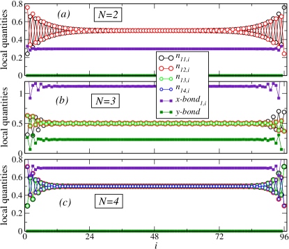
Figure 2: (Color online) Local densities and bond energies obtained by DMRG for a chain of length $L=96$ in the cases $N=2$, $3$ and $4$, using $t_{\perp}=1$, $U=12$, $V=4$. The densities and $x$-bond (i.e., rung) energies are found to be equal on both chains, and we show them for $\ell=1$. The clear evidence of edge states signals the three SPT phases.

The possible SPT phases in the $N=3$ and $N=4$ cases can also be probed using their particular edge states [Fig. 2(b,c)], or their corresponding entanglement spectra (ES) [Fig. 3(b,c)]. The precise nature of the edge states can be inferred from Fig. 2 and, for SU(3), we find that the phase for $t=t_{\perp}=1$ is a $\chi$H phase $(n_{\text{Y}}(\mathcal{R}),n_{\text{Y}}(\bar{\mathcal{R}}))=(1,2)$ with the left and right edge states respectively transforming in the ${\bf 3}$ and ${\bf\bar{3}}$ representations of SU(3) supp . As has been mentioned above, when the system is inversion-symmetric, this and the second $\chi$H phase $(2,1)$ must be degenerate; DMRG simulations randomly pick one of the two minimally entangled states. In fact, we found that another run with a different sweeping procedure gave access to the second one supp . This signals the emergence of the $\chi$H phase $(1,2)$ or $(2,1)$ for $t=t_{\perp}=1$ which spontaneously breaks the inversion symmetry Furusaki2014 ; greiter . Similarly, for $N=4$, the edge states in Fig. 2(c) strongly suggest one of the three SPT phases $(2,2)$ protected by SU(4). Specifically, the edge states are found to belong to the self-conjugate antisymmetric representation of SU(4) with dimension 6, in agreement with previous studies on the $N=4$ case Capponi-L-T-15 ; Nonne-M-C-L-T-13 ; Bois-C-L-M-T-15 ; Totsuka-15 .

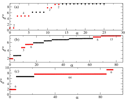
Figure 3: (Color online) The ES obtained by DMRG on $L=48$ chain in the $N=2$, $3$ and $4$ model (from top to bottom) using $t_{\perp}=1$, $U=20$, $V=2$. In all three cases, the system is in the SPT phase. Bosonic (fermionic) levels are shown by red (black) circles. Numbers denote the number of quasi-degenerate levels.

In order to provide additional insight into these SPT phases, we plot their ES obtained by cutting the chain in the middle and computing the Schmidt eigenvalues of the ground-state wavefunction. The ES of the SH phase is known to exhibit double-degeneracy for all levels Pollmann2010 , which is a signature of the underlying SPT phase. Figure 3(a) shows the correct even-fold degeneracy in the low-lying part of the entanglement spectrum, which further confirms the presence of the SH phase. A remark is in order about the interpretation of ES shown in Fig. 3. Since our ES are obtained for the fermionic model (4), some of the higher-lying levels belong to the “fermionic sector” of the spectrum and may not exhibit the structure expected in bosonic SPT phases, as is demonstrated in, e.g., Refs. Hasebe-T-13 ; Pollmann2015 . To resolve this, we separate the bosonic sector (shown by red circles) from the fermionic one (black circles) in Fig. 3. The degeneracy structure of the bosonic sector now perfectly agrees with what we expect for the corresponding SPT phases. In view of the recent developments in entanglement measurements in cold-atom settings Islam-et-al-entanglement-15 , our proposal would make precise characterization of SPT phases possible in experiments. In order to show that the SU($N$) SPT phases found above are not restricted to the strong-coupling regime, we plot their extent as a function of $U$ along the physical line $U/V=10$ in Fig. 4 at fixed $t_{\perp}=t(=1)$. These phases occur in the large-$U$ regime and, for weaker interactions, quantum phase transitions are expected towards fully gapped trivial or dimerized phases which break the translation symmetry spontaneously.

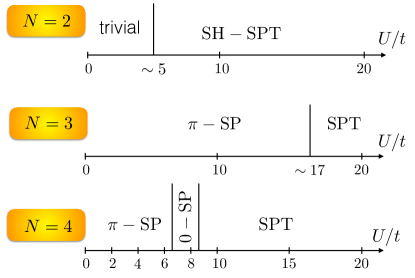
Figure 4: (Color online) Phase diagram for $N=2$, $3$ and $4$ at fixed $t_{\perp}=t=1$, as a function of $U$ (with $U/V=10$, see text) obtained from DMRG simulations. In all three cases, we find different SPT phases at strong coupling. For weaker interactions, we find trivial non-degenerate gapped phases, or the out-of-phase (respectively in-phase) dimerized spin-Peierls-like $\pi$-SP (respectively $0$-SP) phase.

Summary and experimental prospects – We have introduced a simple one-dimensional microscopic model to describe alkali or alkaline-earth ultracold fermionic atoms loaded into a bichromatic optical lattice. Using analytical and numerical insight, we have shown how SU($N$) SPT phases can emerge in a large range of parameters. This provides a physical route to realize the SH phase ($N=2$), its generalization for even $N$, as well as the $\chi$H phase with $N=3$ which breaks spontaneously the inversion symmetry. The experimental realization of the SH phase with $N=2$ may be obtained using the two lowest hyperfine states of ${}^{6}\mathrm{Li}$. In this case, the ratio $U/t$ may be tuned using the broad Feshbach resonance involving these two states zurn_PRL2013 . Furthermore, detection resolved in both density and spin is possible by combining a Fermi-gas microscope with Stern-Gerlach techniques as done in Ref. boll_Science2016 or by ejecting unwanted spin states using resonant pulses as in Ref. parsons_Science2016 . The typical temperature scale of recent experiments with ${}^{6}\mathrm{Li}$ atoms is $T\simeq(0.5-0.8)4t^{2}/U$ boll_Science2016 . Interestingly enough, this temperature scale is of the same order of magnitude as the gap of the SH phase DMRG : $\Delta_{\rm SH}\simeq 0.41J\simeq 0.8t^{2}/U$ obtained in the large-$U$ limit. As was recently shown numerically in Ref. Becker2017 , the main characteristics of the thermal spectral functions of the SH phase with localized edge states are still visible at finite size for $T\simeq\Delta_{\rm SH}$, a temperature scale which is within the reach of forthcoming experiments. Larger values of $N$ are experimentally accessible using fermionic alkaline-earth or ytterbium atoms. Using typical experimental values for ${}^{173}\mathrm{Yb}$ which corresponds to the case of $N=6$ (scattering length $a_{g}=10.55\,\mathrm{nm}$ kitagawa:PRA2008 and lattice spacing $\pi/k\approx 400\,\mathrm{nm}$ hofrichter:PRX2016 ), we find $U/V\sim 10$. Spin-resolved measurements may be performed on these systems using optical Stern–Gerlach techniques stellmer_PRA2011 . In the light of the recent experimental achievements with cold fermionic quantum gases, we expect the SPT phases discussed in this Letter to be observed in the near future.

Supplemental Materials: “Haldane” phases with ultracold fermionic atoms in double–well optical lattices

I Strong-coupling expansion for SU(3)

In this section, we consider the strong-coupling limit of SU($N$) cold fermions confined in a double-well optical lattice described by the following Hubbard-like Hamiltonian:

$$\begin{split}{\cal H}=&-t\sum_{i}\sum_{\ell=1}^{2}\sum_{\alpha=1}^{N}\left(c_{\ell\alpha,i+1}^{\dagger}c_{\ell\alpha,i}+\text{H.c.}\right)-t_{\perp}\sum_{i}\sum_{\alpha=1}^{N}\left(c_{1\alpha,i}^{\dagger}c_{2\alpha,i}+\text{H.c.}\right)-\mu\sum_{i}n_{i}\\ &+\frac{U}{2}\sum_{i}\sum_{\ell=1}^{2}\sum_{\alpha\neq\beta}n_{\ell\alpha,i}n_{\ell\beta,i}\\ &+V\sum_{i}\sum_{\alpha\neq\beta}\biggl{\{}n_{1\alpha,i}n_{2\beta,i}+c_{1\alpha,i}^{\dagger}c_{2\beta,i}^{\dagger}c_{1\beta,i}c_{2\alpha,i}+\frac{1}{2}\left(c_{1\alpha,i}^{\dagger}c_{1\beta,i}^{\dagger}c_{2\beta,i}c_{2\alpha,i}+\text{H.c.}\right)\biggr{\}}\;.\end{split}$$ (S1)

Dropping the inter-chain interactions (i.e., $V=0$), we recover the SU($N$) Hubbard ladder. The atomic limit ($t=0$) of the above Hamiltonian is most conveniently described using the antisymmetric (anti-bonding) and symmetric (bonding) combinations of the $c$-fermions introduced in the Letter:

$$d_{1\sigma,i}=\frac{1}{\sqrt{2}}\left(c_{1\sigma,i}-c_{2\sigma,i}\right)\;,\;\;d_{2\sigma,i}=\frac{1}{\sqrt{2}}\left(c_{1\sigma,i}+c_{2\sigma,i}\right)\;,$$ (S2)

in terms of which the atomic-limit Hamiltonian reads as [$t=0$ limit of Eq. (4) of the Letter]:

$$\begin{split}&\mathcal{H}_{0}=\sum_{i}\mathcal{H}_{\text{on-site}}(i)\\ &\mathcal{H}_{\text{on-site}}(i)=-\left(\mu+\frac{U+V}{2}\right)n_{i}+2t_{\perp}T_{i}^{z}+\frac{U+V}{4}n_{i}^{2}+2V(T_{i}^{z})^{2}+(U-V)(T_{i}^{x})^{2}\;.\end{split}$$ (S3)

The orbital pseudo-spin $\mathbf{T}$ is defined with respect to the $d$-fermions: $T_{i}^{a}=\frac{1}{2}\sum_{m,n,\alpha}d_{m\alpha,\,i}^{\dagger}\sigma^{a}_{mn}d_{n\alpha,\,i}$. Note that the hopping between the two wells ($\ell=1,2$) now translates to the number difference: $t_{\perp}(n^{(d)}_{1,i}-n^{(d)}_{2,i})$. The spectrum of $\mathcal{H}_{\text{on-site}}$ (S3) is labeled by various quantum numbers, i.e., (i) the total number of particle $n_{i}$, (ii) the orbital pseudo-spin squared $\mathbf{T}_{i}^{2}=T(T+1)$ ($T^{z}$ is not a good quantum number in general) as well as (iii) the SU($N$) irreducible representations which are most conveniently specified by Young diagrams with at most two columns Itzykson and Nauenberg (1966); Georgi (1999). Although the on-site part of the Hamiltonian does not contain SU($N$)-dependent interactions, the optimal SU($N$) representation is selected by the orbital($\mathbf{T}$)-dependent part through the Fermi statistics (see, e.g., Appendix A of Ref. Bois et al. (2015)). The condition of half filling is imposed by setting

$$\mu=\frac{N}{2}(U+V)$$ (S4)

for which the spectrum exhibits the particle-hole symmetry: $n\leftrightarrow 2N-n$. To ease the notations, we will drop the site index for the on-site limit spectrum.

I.1 Atomic-limit spectrum

The atomic-limit Hamiltonian (S3) commutes with the SU($N$) generators and the orbital pseudo-spin $\mathbf{T}$, we can diagonalize it for given SU($N$) representation and $\mathbf{T}$. Due to the fermionic statistics, only special combinations of SU($N$) representations and $\mathbf{T}$ appear for a given local fermion number $n$ ($0\leq n\leq 2N$) Bois et al. (2015):

$$\yng(1)\sim(\underbrace{\yng(1)}_{\text{SU}(N)},\underbrace{\yng(1)}_{\text{SU(2)}})\quad(n=1)$$ (S5a)

$$\yng(1,1)\sim\left(\yng(2),\bullet\right)\oplus\left(\yng(1,1),\yng(2)\right)\quad(n=2)$$ (S5b)

$$\yng(1,1,1)\sim\left(\yng(2,1),\yng(1)\right)\oplus\left(\yng(1,1,1),\yng(3)\right)\quad(n=3)$$ (S5c)

$$\yng(1,1,1,1)\sim\left(\yng(2,2),\bullet\right)\oplus\left(\yng(2,1,1),\yng(2)\right)\oplus\left(\yng(1,1,1,1),\yng(4)\right)\quad(n=4)$$ (S5d)

$$\yng(1,1,1,1,1)\sim\left(\yng(2,2,1),\yng(1)\right)\oplus\left(\yng(2,1,1,1),\yng(3)\right)\oplus\left(\yng(1,1,1,1,1),\yng(5)\right)\quad(n=5)$$ (S5e)

$$\qquad\qquad\qquad\vdots$$

$$\text{\scriptsize$2N$}\left\{\yng(1,1,1,1,1)\right.\sim\left(\bullet,\bullet\right)\quad(n=2N)$$ (S5f)

As the Hamiltonian (S3) does not depend on SU($N$), given $n$, we just diagonalize (S3) for all allowed $T$.

When $N=3$, the fermion number can take $n=0,1,\ldots,6\,(=2N)$. The energy-spectrum for the fermion number $n$ is given by:

$$E_{n=0,6}(\bullet,T=0)=0$$ (S6a)

$$E_{n=1,5}((\mathbf{3},\bar{\mathbf{3}}),T=1/2)=\begin{cases}t_{\perp}-\left(U+V\right)&(T^{z}=+1/2;\times 3)\\ -t_{\perp}-\left(U+V\right)&(T^{z}=-1/2;\times 3)\end{cases}$$ (S6b)

$$E_{n=2,4}((\mathbf{6},\bar{\mathbf{6}}),T=0)=-2\left(U+V\right)\;(\times 6)$$ (S6c)

$$E_{n=2,4}((\bar{\mathbf{3}},\mathbf{3}),T=1)=\begin{cases}-\frac{3}{2}U-\frac{1}{2}V-\sqrt{4t_{\perp}^{2}+\left(\frac{U-V}{2}\right)^{2}}&(\times 3)\\ -\frac{3}{2}U-\frac{1}{2}V+\sqrt{4t_{\perp}^{2}+\left(\frac{U-V}{2}\right)^{2}}&(\times 3)\\ -U-3V&(T^{z}=0;\times 3)\end{cases}$$ (S6d)

$$E_{n=3}(\mathbf{8},T=1/2)=\begin{cases}t_{\perp}-2(U+V)&T^{z}=+1/2\;\;(\times 8)\\ -t_{\perp}-2(U+V)&T^{z}=-1/2\;\;(\times 8)\end{cases}$$ (S6e)

$$E_{n=3}(\bullet,T=3/2)=\begin{cases}t_{\perp}-U-V-\sqrt{4t_{\perp}^{2}-2t_{\perp}U+U^{2}+10t_{\perp}V-4UV+7V^{2}}&\\ t_{\perp}-U-V+\sqrt{4t_{\perp}^{2}-2t_{\perp}U+U^{2}+10t_{\perp}V-4UV+7V^{2}}&\\ -t_{\perp}-U-V-\sqrt{4t_{\perp}^{2}+2t_{\perp}U+U^{2}-10t_{\perp}V-4UV+7V^{2}}&\\ -t_{\perp}-U-V+\sqrt{4t_{\perp}^{2}+2t_{\perp}U+U^{2}-10t_{\perp}V-4UV+7V^{2}}&,\end{cases}$$ (S6f)

where the irreducible representations of the SU(3) group are labeled by their dimension:

$$\begin{split}&\mathbf{3}\;\leftrightarrow\;\yng(1)\;,\;\;\bar{\mathbf{3}}\;\leftrightarrow\;\yng(1,1)\;,\\ &\mathbf{6}\;\leftrightarrow\;\yng(2)\;,\;\bar{\mathbf{6}}\;\leftrightarrow\;\yng(2,2)\\ &\mathbf{8}\;\leftrightarrow\;\yng(2,1)\;.\end{split}$$ (S7)

The lowest of these energies for different parameters ($U,V$) are displayed in Fig. (S1).

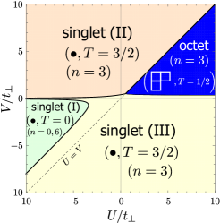
Figure S1: Atomic-limit phase diagram of $\mathcal{H}_{\text{on-site}}$ for $N=3$. There are four phases: (i) SU(3) octet phase with $n=3$, $\mathbf{8}$ (adjoint), and $(T=1/2,T^{z}=-1/2)$ [blue; second of Eq. (S6e)], (ii) SU(3)-singlet phase (I) with $n=0$ or $6$, $\bullet$, and $T=0$ [green; Eq. (S6a)], (iii) SU(3)-singlet phase (II) with $n=3$, $\bullet$, and $T=3/2$ [pale orange; first of Eq. (S6f)], and (iv) SU(3)-singlet phase (III) with $n=3$, $\bullet$, and $T=3/2$ [pale yellow; third of Eq. (S6f)]. The SU(3)-singlet phase (I) suggests that a period-2 charge-density wave might be stabilized there. Chemical potential is fixed to $\mu=3(U+V)/2$.

I.2 Effective Hamiltonian for octet phase

Now let us consider the octet phase (shown by blue in Fig. S1) where an SU(3) “magnetic moment” in the $\mathbf{8}$ (adjoint) representation is formed at each rung (i.e., double well) and the orbital pseudo-spin $\mathbf{T}$ is quenched to $T=1/2,T^{z}=-1/2$. In this phase, the low-energy effective Hamiltonian is expected to be SU(3)-invariant and written only in terms of the SU(3) “spins” in $\mathbf{8}$. First, we restrict the form of possible interactions by symmetry consideration. From the Clebsch-Gordan decomposition

$$\begin{split}&\yng(2,1)\otimes\yng(2,1)\quad\simeq\quad\underbrace{\yng(4,2)}_{\mathbf{27}}\;\oplus\;\underbrace{\yng(3)}_{\mathbf{10}}\;\oplus\;\underbrace{\yng(3,3)}_{\overline{\mathbf{10}}}\;\oplus\;\underbrace{\yng(2,1)}_{\mathbf{8}_{\text{S}}}\;\oplus\;\underbrace{\yng(2,1)}_{\mathbf{8}_{\text{A}}}\;\oplus\;\bullet\\ &(\mathbf{8}\times\mathbf{8}=\mathbf{27}\oplus\mathbf{10}\oplus\overline{\mathbf{10}}\oplus\mathbf{8}_{\text{S}}\oplus\mathbf{8}_{\text{A}}\oplus\mathbf{1})\;,\end{split}$$ (S8)

(the subscripts “S” and “A” label the two $\mathbf{8}$ representations) one sees (by the Schur’s lemma) that any SU(3)-invariant (two-site) interactions can be completely parametrized by six independent coefficients corresponding to the six irreducible representations appearing on the right-hand side:

$$a_{\mathbf{27}}P_{\mathbf{27}}+a_{\mathbf{10}}P_{\mathbf{10}}+a_{\overline{\mathbf{10}}}P_{\overline{\mathbf{10}}}+a_{\mathbf{8}_{\text{S}}}P_{\mathbf{8}_{\text{S}}}+a_{\mathbf{8}_{\text{A}}}P_{\mathbf{8}_{\text{A}}}+a_{\mathbf{1}}P_{\mathbf{1}}$$ (S9)

with $P_{R}$ being the projection operator onto the irreducible represenation $R$ and $a_{R}$ the corresponding real coefficient. In the case of SU(2), the projection operators are uniquely expressed in terms of polynomials of the quadratic Casimir $\mathcal{C}_{2}$ (or, $\mathbf{S}_{1}{\cdot}\mathbf{S}_{2}$). On the other hand, in SU($N$) ($N\geq 3$), higher-order Casimirs and other operators may also be necessary to recast the general form (S9) into the “spin” Hamiltonian. Specifically, for a pair of SU(3) spins $\mathcal{S}_{1}^{A}$, $\mathcal{S}_{2}^{B}$ in $\mathbf{8}$, the most general SU(3)-invariant two-site interaction may be written as:

$${\cal H}^{(\text{octet})}_{\text{eff}}=\alpha\mathbf{1}+J_{1}\sum_{A}\mathcal{S}^{A}_{1}\mathcal{S}^{A}_{2}+J_{2}\left(\sum_{A}\mathcal{S}^{A}_{1}\mathcal{S}^{A}_{2}\right)^{2}+J_{3}\left(\sum_{A}\mathcal{S}^{A}_{1}\mathcal{S}^{A}_{2}\right)^{3}+J_{4}\mathcal{C}_{3}(\mathcal{S}_{1},\mathcal{S}_{2})+p\mathcal{P}_{\mathbf{8},\mathbf{8}},$$ (S10)

where $\mathcal{P}_{\mathbf{8},\mathbf{8}}$ is the permutation operators of the neighboring sites 1 and 2, and $\mathcal{C}_{3}$ is the cubic Casimir made of $\mathcal{S}_{1,2}^{A}$. The “exchange interaction” $\sum_{A=1}^{8}\mathcal{S}^{A}_{1}\mathcal{S}^{A}_{2}$ is directly related to the quadratic Casimir as:

$$\begin{split}\sum_{A=1}^{8}\mathcal{S}^{A}_{1}\mathcal{S}^{A}_{2}&=\sum_{A}\frac{1}{2}\left\{\left(\mathcal{S}^{A}_{1}+\mathcal{S}^{A}_{2}\right)^{2}-\left(\mathcal{S}^{A}_{1}\right)^{2}-\left(\mathcal{S}^{A}_{2}\right)^{2}\right\}\\ &=\frac{1}{2}\left\{\mathcal{C}_{2}(R)-2\mathcal{C}_{2}(\mathbf{8})\right\},\end{split}$$ (S11)

which enables us to use $\sum_{A=1}^{8}\mathcal{S}^{A}_{1}\mathcal{S}^{A}_{2}$ instead of the full quadratic Casimir operator. The reason for the necessity of $\mathcal{P}_{\mathbf{8},\mathbf{8}}$ is that the two adjoint representations $\mathbf{8}$ share the same set of the Casimirs $(\mathcal{C}_{2},\mathcal{C}_{3})$ (see Table 1) and are distinguished only by $\mathcal{P}_{\mathbf{8},\mathbf{8}}$. As $\mathcal{C}_{3}$ is odd under the conjugation $R\to\overline{R}$ (which, in the fermion language, translates to the particle-hole transformation), $J_{4}=0$ at half-filling.

Second-order processes in $t$ give an effective interaction between a pair of SU(3) spins in $\mathbf{8}$, whose coupling constants $\{\alpha,J_{1},J_{2},J_{3},p\}$ are given in terms of $(t,t_{\perp},U,V)$ as:

$$\alpha=\frac{1}{6}\left(\frac{A}{6}-\frac{B}{2}\right)$$ (S12a)

$$J_{1}=\frac{A}{9}+\frac{2B}{9}\,,\;\;J_{2}=-\frac{10}{27}\left(A-B\right)\,,\;\;J_{3}=-\frac{2}{27}\left(A-B\right)$$ (S12b)

$$p=\frac{1}{6}\left(A-B\right),$$ (S12c)

where

$$\begin{split}A&\equiv\frac{t^{2}\left(8t_{\perp}+3U+V\right)}{U\left(U+V\right)+t_{\perp}\left(3U+V\right)}\\ B&\equiv\frac{3t^{2}\left(8t_{\perp}+U+3V\right)}{V\left(U+V\right)+t_{\perp}\left(U+3V\right)}\;.\end{split}$$ (S12d)

The spectrum of the two-site effective Hamiltonian ${\cal H}_{\text{eff}}$ (S10) reads as:

$$E_{0}\quad(\times 27;\;\;\mathbf{27})$$ (S13a)

$$E_{0}-\frac{B}{3}\quad(\times 20;\;\;\mathbf{10},\overline{\mathbf{10}})$$ (S13b)

$$E_{0}-\frac{4A}{3}\quad(\times 1;\;\;\mathbf{1})$$ (S13c)

$$E_{0}-\frac{5(A+B)}{12}\quad(\times 8;\;\mathbf{8}_{\text{S}})\,,\;\;E_{0}-\frac{3A}{4}-\frac{B}{12}\quad(\times 8;\;\mathbf{8}_{\text{A}}).$$ (S13d)

with $E_{0}=2E_{n=3}(\mathbf{8},T=1/2)=-2t_{\perp}-4(U+V)$. For values of parameters corresponding to the octet phase of Fig. S1, we have $J_{1}\sim J_{2}$ and we must retain the biquadratic term $\left(\sum_{A}\mathcal{S}^{A}_{1}\mathcal{S}^{A}_{2}\right)^{2}$, and hence nothing more can be said about the physics described without a direct numerical investigation of the effective Hamiltonian (S10). Furthermore a numerical derivation of the full two-site spectrum shows that the effective Hamiltonian description is valid for $t_{\perp}\gtrsim t$ ($t_{\perp}>1.7t$ in the case of $U=100$, $V=10$ for unit $t$ according to Fig. S2). Given the parameters dependences of $J_{1},J_{2},J_{3}$ and $p$, their values stay qualitatively the same on all the octet region of Fig. S1. Hence Fig. S3 obtained by DMRG for $t_{\perp}=10$, $t=1$, $U=100$, and $V=10$ provides also a valid depiction of the phase described by the effective Hamiltonian (S10) for realistic parameters. One thus concludes that for $N=3$ a featureless fully gapped phase is stabilized without any edge states. However, this description breaks down when $t_{\perp}\lesssim t$, the typical regime where a SPT phase can emerge, as shown below, where we have to use the other approach presented in the Letter.

irreps.	${\tiny\yng(4,2)}$	${\tiny\yng(3)}$	${\tiny\yng(3,3)}$	${\tiny\yng(2,1)}$	${\tiny\yng(2,1)}$	$\bullet$
dimensions	$\mathbf{27}$	$\mathbf{10}$	$\overline{\mathbf{10}}$	$\mathbf{8}_{\text{S}}$	$\mathbf{8}_{\text{A}}$	$\mathbf{1}$
quadratic Casimir $\mathcal{C}_{2}$	8	6	6	3	3	0
cubic Casimir $\mathcal{C}_{3}$	0	9	$-9$	0	0	0
symmetry ($\mathcal{P}_{\mathbf{8},\mathbf{8}}$)	$1$	$-1$	$-1$	$1$	$-1$	$1$

Table 1: Quadratic and cubic Casimirs for the six irreducible representations appearing in the decomposition of $\mathbf{8}\otimes\mathbf{8}$ [eq.(S8)].

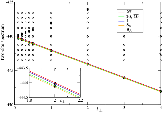
Figure S2: Exact two-site spectrum for $U=100$, $V=10$ and unit $t$ versus $t_{\perp}$. The spectrum (S13) predicted by the effective Hamiltonian (S10) is drawn in color lines. A zoom on the ground states around $t_{\perp}=2$ is provided on the bottom left corner. The effective Hamiltonian description breaks down for $t_{\perp}<1.7t$.

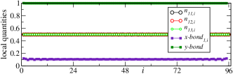
Figure S3: Local quantities for the $N=3$ model obtained by DMRG simulations for $L=96$, $(U,V)=(100,10)$ and $t_{\perp}/t=10$.

II Numerical results

II.1 Edge states in $N=3$ model

As is well-known, the sharpest characterization of (bosonic) SPT phases is obtained by analyzing the projective representation appearing at the edges (whether physical or virtual). Nevertheless, for practical purposes, the observation of the physical edge states still provides us with a useful method of accessing the underlying topological properties (especially when we consider bosonic SPT phases realized in fermionic systems). To demonstrate how this strategy works, let us consider the two SU(3) valence-bond solid (VBS) states Affleck et al. (1988) and calculate the expectation values of the two Cartan generators $G^{3}_{r}$ and $G^{8}_{r}$ in the 8-dimensional adjoint representation ($\mathbf{8}$) at site $r$ (the SU(3) generators are normalized as $\text{Tr}G^{A}G^{B}=6\delta^{AB}$). The two VBS states break the reflection symmetry spontaneously and are known Morimoto et al. (2014) to belong to the two different SPT phases predicted by group cohomology Duivenvoorden and Quella (2013) (see Fig. S4).

We begin with the $(\mathbf{3},\bar{\mathbf{3}})$ VBS state shown in Fig. S4(a). Using the matrix-product state formalism, it is straightforward to calculate the local expectation values of $G^{3}_{r}$ and $G^{8}_{r}$ for a semi-infinite system (we have chosen a semi-infinite system just to suppress the effects from the other edge):

$$\left(\langle G^{3}_{r}\rangle,\langle G^{8}_{r}\rangle\right)=\begin{cases}\left(-\frac{9}{\sqrt{2}}\left(-\frac{1}{8}\right)^{r},-\frac{3\sqrt{3}}{\sqrt{2}}\left(-\frac{1}{8}\right)^{r}\right)&\text{for L-edge state 1}\\ \left(+\frac{9}{\sqrt{2}}\left(-\frac{1}{8}\right)^{r},-\frac{3\sqrt{3}}{\sqrt{2}}\left(-\frac{1}{8}\right)^{r}\right)&\text{for L-edge state 2}\\ \left(0,3\sqrt{6}\left(-\frac{1}{8}\right)^{r}\right)&\text{for L-edge state 3}\;.\end{cases}$$ (S14)

Summing up these values, we obtain the edge moment localized around the left edge:

$$\sum_{r=1}^{\infty}\left(\langle G^{3}_{r}\rangle,\langle G^{8}_{r}\rangle\right)=\begin{cases}\left(\frac{1}{\sqrt{2}},\frac{1}{\sqrt{6}}\right)=\lambda_{\text{\bf 3}}(1)&\text{for L-edge state 1 (heighest weight state (hws) of $\mathbf{3}$)}\\ \left(-\frac{1}{\sqrt{2}},\frac{1}{\sqrt{6}}\right)=\lambda_{\text{\bf 3}}(2)&\text{for L-edge state 2}\\ \left(0,-\sqrt{\frac{2}{3}}\right)=\lambda_{\text{\bf 3}}(3)&\text{for L-edge state 3}\end{cases}$$ (S15)

which is to be compared with the SU(3) weights of $\mathbf{3}$ shown in Fig. S5 (a). A similar calculation leads us to the following set of weights at the right edge:

$$\sum_{r=\text{right edge}}\left(\langle G^{3}_{r}\rangle,\langle G^{8}_{r}\rangle\right)=\begin{cases}\left(-\frac{1}{\sqrt{2}},-\frac{1}{\sqrt{6}}\right)=\lambda_{\bar{\text{\bf 3}}}(1)&\text{for R-edge state 1}\\ \left(\frac{1}{\sqrt{2}},-\frac{1}{\sqrt{6}}\right)=\lambda_{\bar{\text{\bf 3}}}(2)&\text{for R-edge state 2 (hws of $\bar{\mathbf{3}}$)}\\ \left(0,\sqrt{\frac{2}{3}}\right)=\lambda_{\bar{\text{\bf 3}}}(3)&\text{for R-edge state 3}\;,\end{cases}$$ (S16)

which then implies that $\bar{\mathbf{3}}$ appears at the right edge. (For the other topological VBS state $(\bar{\mathbf{3}},\mathbf{3})$, we just obtain the weights with $\mathbf{3}$ and $\bar{\mathbf{3}}$ interchanged.)

In the Letter, we have shown that, in some region of the Mott-insulating phase, the above SU(3) SPT phases are stabilized. In the region, we may expect that the following fermion operators reduce to the SU(3) “spins” $G_{r}^{A}$ in $\mathbf{8}$:

$$\begin{split}\widehat{G}_{r}^{A}&=\sum_{\alpha,\beta=1}^{3}c_{1\alpha,r}^{\dagger}\left(G^{A}\right)_{\alpha\beta}c_{1\beta,r}+\sum_{\alpha,\beta=1}^{3}c_{2\alpha,r}^{\dagger}\left(G^{A}\right)_{\alpha\beta}c_{2\beta,r}\\ &=\sum_{\alpha,\beta=1}^{3}d_{1\alpha,r}^{\dagger}\left(G^{A}\right)_{\alpha\beta}d_{1\beta,r}+\sum_{\alpha,\beta=1}^{3}d_{2\alpha,r}^{\dagger}\left(G^{A}\right)_{\alpha\beta}d_{2\beta,r}\quad(A=3,8)\\ &=\begin{cases}\frac{1}{\sqrt{2}}(n_{r}(1)-n_{r}(2))&A=3\\ \frac{1}{\sqrt{6}}(n_{r}(1)+n_{r}(2)-2n_{r}(3))&A=8\;,\end{cases}\end{split}$$ (S17)

where $n_{r}(\alpha)=\sum_{\ell=1,2}c_{\ell\alpha,r}^{\dagger}c_{\ell\alpha,r}=\sum_{\ell=1,2}d_{\ell\alpha,r}^{\dagger}d_{\ell\alpha,r}$.

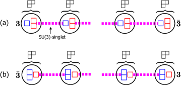
Figure S4: Two SU(3) VBS states that break reflection symmetry spontaneously. They are distinguished by the edge states: in (a), $\mathbf{3}$ and $\bar{\mathbf{3}}$ respectively appear at the left and right edges, while, in (b), $\mathbf{3}$ and $\bar{\mathbf{3}}$ are interchanged. We call these VBS states $(\mathbf{3},\bar{\mathbf{3}})$ [(a)] and $(\bar{\mathbf{3}},\mathbf{3})$ [(b)].

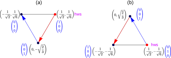
Figure S5: Weights of 3 representation ($\mathbf{3}$) and its conjugate ($\bar{\mathbf{3}}$). Red (blue) arrows denote the action of simple root $-\boldsymbol{\alpha}_{1}$ ($-\boldsymbol{\alpha}_{2}$).

Figure S6: Weights 8-dimensional (adjoint) representation. The weight $(0,0)$ is doubly degenerate [corresponding to the two Cartan generators of SU(3)]. Red (blue) arrows denote the action of simple root $-\boldsymbol{\alpha}_{1}$ ($-\boldsymbol{\alpha}_{2}$).

In the SU(3) SPT phase, we thus expect an overall $2\times 3\times 3=18$ degeneracy of the ground-state corresponding to all possible edge states as well as inversion symmetry. In a numerical DMRG simulation, it is well-known that the algorithm will converge to one of these ground-states randomly (i.e. convergence depends on the sweeping procedure and other details). Note also that since we are implementing U(1) quantum numbers corresponding to the color conservation, left- and right-edge states are related so that $(G^{3}_{\mathrm{tot}},G^{8}_{\mathrm{tot}})=(0,0)$, which reduces the degeneracy to $2\times 3=6$. In order to characterize a given edge states, we can simply use the local densities $n_{\ell\alpha,i}$ to compute quantities in Eqs. (S15)-(S16). For instance, the data presented in Fig. 2 of the main text for $N=3$ correspond to a left-edge having $\lambda_{\bar{\text{\bf 3}}}(1)$.

In order to further reduce the degeneracy, we can also work in a “polarized” case (by analogy with the spin-1 case for instance) by fixing the total number of particles per color as $(n_{1},n_{2},n_{3})=(L+1,L-1,L)$ so that $(G^{3}_{\mathrm{tot}},G^{8}_{\mathrm{tot}})=(\sqrt{2},0)$ for which there are only two candidates, namely left-edge having $\lambda_{\text{\bf 3}}(1)$ and right-edge $\lambda_{\bar{\text{\bf 3}}}(2)$, or vice-versa. In Fig. S7, we provide two different of set of parameters corresponding to these two possible ground-states, hence showing explicitly the inversion symmetry breaking.

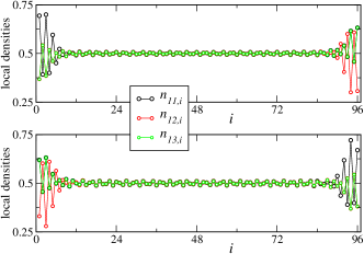
Figure S7: Local densities for the $N=3$ model obtained by DMRG simulations for $L=96$, $t=t_{\perp}=1$ and $(U,V)=(20,2)$ (top) or $(U,V)=(100,10)$ (bottom) respectively. We fix the total number of particles per color as $(n_{1},n_{2},n_{3})=(L+1,L-1,L)$ and we do observe the two possible edge states (corresponding to the two ground-states in this sector, see text). Top: left-edge has $\lambda_{\bar{\text{\bf 3}}}(1)$ and right-edge $\lambda_{\bar{\text{\bf 3}}}(2)$. Bottom: opposite situation showing the inversion symmetry breaking.

II.2 Entanglement spectrum in finite-size systems

In the Letter, we have used the structure of the entanglement spectrum to identify the topological properties underlying the ground-state wave function. However, our calculations were done for finite-size systems and it is not obvious to what extent the theoretical predictions, that are made using the properties of infinite-size matrix-product states Pérez-García et al. (2008); Pollmann et al. (2010); Tanimoto and Totsuka , are valid. To illustrate how finite-size calculations work in getting getting the information on the topological properties, we calculate the entanglement spectrum (i.e., the Schmidt eigenvalues) of the $(\mathbf{3},\bar{\mathbf{3}})$ VBS state Affleck et al. (1988); Morimoto et al. (2014) discussed above. Following the standard procedure Shi et al. (2006), we can obtain the entanglement spectrum for a finite-size ($L$) system:

$$\frac{\sqrt{1+2(-1/8)^{\ell_{\text{L}}}}\sqrt{1+2(-1/8)^{\ell_{\text{R}}}}}{\sqrt{3}\sqrt{1+2(-1/8)^{L}}}\;,\;\;\frac{\sqrt{1-(-1/8)^{\ell_{\text{L}}}}\sqrt{1-(-1/8)^{\ell_{\text{R}}}}}{\sqrt{3}\sqrt{1+2(-1/8)^{L}}}\;\;(\times 2)\;,$$ (S18)

where $\ell_{\text{L}}$ and $\ell_{\text{R}}$ respectively are the sizes of the left and right subsystems ($L=\ell_{\text{L}}+\ell_{\text{R}}$), and the edge states are fixed to $\lambda_{\text{\bf 3}}(1)$ (left) and $\lambda_{\bar{\text{\bf 3}}}(1)$ (right). For finite-size systems, the three-fold degeneracy, which is a clear signature of the topological property, is weakly broken (with an exponentially small splitting). Roughly, the fictitious SU(3) spins $\mathbf{3}$ and $\bar{\mathbf{3}}$ at the entanglement cut feel the (exponentially small) effects of the actual (emergent) edge spins on the boundaries thereby breaking the perfect degeneracy characteristic of free spins.

II.3 Quantum phase transition induced by $t_{\perp}$ in the $N=3$ model

As discussed in the strong coupling section above, the effective model is highly non-trivial for $N=3$ and in particular, there is a crucial role played by $t_{\perp}$ which acts as an effective magnetic field for the $d$ orbitals. In Fig. S3 and Fig. S8 , we plot the local quantities (see main text) for large interactions and various $t_{\perp}$, so that we can identify several phases. At small $t_{\perp}/t=0.4$, one clearly observes in-phase dimerization, corresponding to a uniform spin Peierls-like phase $0$-SP. When $t_{\perp}=t$, we recover the $N=3$ chiral SPT phase, which in this particular simulation corresponds to a left-edge having $\lambda_{\text{\bf 3}}(2)$ (hence a right-edge corresponding to $\lambda_{\bar{\text{\bf 3}}}(2)$). Finally, for large $t_{\perp}/t=10$, there is a quantum phase transition to a featureless fully gapped phase. Note that in this case, the rung energy is very close to $1$, as expected when orbital fluctuations are suppressed.

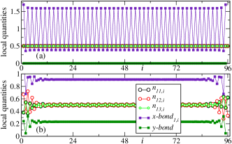
Figure S8: Local quantities for the $N=3$ model obtained by DMRG simulations for $L=96$, $(U,V)=(100,10)$ and varying $t_{\perp}/t=0.4$ (a) and $1$ (b) respectively.

References

- Itzykson and Nauenberg (1966) C. Itzykson and M. Nauenberg, Rev. Mod. Phys. 38, 95 (1966).
- Georgi (1999) H. Georgi, Lie Algebras in Particle Physics (Perseus Books, 1999).
- Bois et al. (2015) V. Bois, S. Capponi, P. Lecheminant, M. Moliner, and K. Totsuka, Phys. Rev. B 91, 075121 (2015).
- Affleck et al. (1988) I. Affleck, T. Kennedy, E. H. Lieb, and H. Tasaki, Comm. Math. Phys. 115, 477 (1988), 10.1007/BF01218021.
- Morimoto et al. (2014) T. Morimoto, H. Ueda, T. Momoi, and A. Furusaki, Phys. Rev. B 90, 235111 (2014).
- Duivenvoorden and Quella (2013) K. Duivenvoorden and T. Quella, Phys. Rev. B 87, 125145 (2013).
- Pérez-García et al. (2008) D. Pérez-García, M. M. Wolf, M. Sanz, F. Verstraete, and J. I. Cirac, Phys. Rev. Lett. 100, 167202 (2008).
- Pollmann et al. (2010) F. Pollmann, A. M. Turner, E. Berg, and M. Oshikawa, Phys. Rev. B 81, 064439 (2010).
- (9) K. Tanimoto and K. Totsuka, ArXiv:1508.07601.
- Shi et al. (2006) Y.-Y. Shi, L.-M. Duan, and G. Vidal, Phys. Rev. A 74, 022320 (2006).