Perturbed angular distributions with LaBr₃ detectors: the $\bm{g}$ factor of the first $\bm{10^{+}}$ state in ¹¹⁰Cd revisited

Abstract

The Time Differential Perturbed Angular Distribution technique with LaBr₃ detectors has been applied to the $I^{\pi}=\frac{11}{2}^{-}$ isomeric state ($E_{x}=846$ keV, $\tau=107$ ns) in ¹⁰⁷Cd, which was populated and recoil-implanted into a gadolinium host following the ⁹⁸Mo(¹²C, $3n$)¹⁰⁷Cd reaction. The static hyperfine field strength of Cd recoil implanted into gadolinium was thus measured, together with the fraction of nuclei implanted into field-free sites, under similar conditions as pertained for a previous implantation perturbed angular distribution $g$-factor measurement on the $I^{\pi}=10^{+}$ state in ¹¹⁰Cd. The ¹¹⁰Cd $g(10^{+})$ value was thereby re-evaluated, bringing it into agreement with the value expected for a seniority-two $\nu h_{\nicefrac{{11}}{{2}}}$ configuration.

I Introduction

The recent development of Lanthanum Bromide (LaBr₃) scintillator detectors provides an opportunity to perform perturbed angular distribution $g$-factor measurements under new experimental conditions. In such measurements, the time-dependent spin-rotation of a nuclear state subjected to a known magnetic field can be observed to deduce the nuclear $g$ factor. One limitation of time-differential techniques is the maximum frequency that can be resolved by the experimental system. High-purity germanium (HPGe) detectors are commonly used for in-beam spectroscopy due to their excellent energy resolution. However, the time resolution of HPGe detectors (${\sim}10$ ns) is insufficient for many time-differential measurements Mihailescu et al. (2007); Crespi et al. (2010). In particular, HPGe detectors cannot be used in cases that use strong hyperfine magnetic fields with resultant high precession frequencies corresponding to periods $\lesssim 10$ ns.

LaBr₃ detectors have excellent time resolution (${\sim}300$ ps is readily achievable Iltis et al. (2006); Règis et al. (2010); Mason et al. (2013); Alharbi et al. (2013); Roberts et al. (2014); Mărginean et al. (2010); Régis et al. (2009); Zhu et al. (2011)), and energy resolution much superior to other commonly used scintillators such as NaI and BaF₂, making them an excellent choice for fast in-beam Time Differential Perturbed Angular Distribution (TDPAD) measurements Fraile (2017). Thus the new opportunities for application of LaBr₃ detectors include the measurement of ${g}$ factors of shorter-lived nuclear states in known, intense, static hyperfine magnetic fields in magnetic hosts, satisfying the condition $\tau\gtrsim T_{L}=\pi/\omega_{L}$, where $\tau$ is the nuclear mean life, and $T_{L}(\omega_{L})$ is the Larmor period (frequency) Recknagel (1974). Cases where the period $T_{L}$ is of the order of a few nanoseconds become accessible for in-beam measurement. The measurements typically have the target backed by a ferromagnetic foil into which the nuclei of interest are recoil implanted. Available ferromagnetic hosts include iron, nickel, cobalt, and gadolinium. Gadolinium is an advantageous ferromagnetic host due to its higher $Z$, which allows nuclei with $Z\lesssim 60$ to be created in-beam at energies below the Coulomb barrier of the beam on gadolinium, resulting in cleaner $\gamma$-ray spectra.

As a first application of LaBr₃ detectors to in-beam TDPAD techniques, the hyperfine field of Cd implanted into gadolinium has been investigated. The motivation was to revisit the $g$-factor measurement on the $I^{\pi}=10^{+}$ state in ¹¹⁰Cd Regan et al. (1995). Even though the $I^{\pi}=10^{+}$ itself is too short lived ($\tau\sim 1$ ns Piiparinen et al. (1993); Juutinen et al. (1994); Kostov et al. (1998); Harissopulos et al. (2001)) to apply the TDPAD method directly, in-beam TDPAD measurements can determine the effective hyperfine field at Cd nuclei implanted into gadolinium hosts. Additionally, the original measurement was time-integral, and reported $g(10^{+})=-0.09(3)$, at least a factor of two smaller than $g\approx-0.2$ to $-0.3$ that would be expected for a rather pure $(h_{\nicefrac{{11}}{{2}}})^{2}$ neutron configuration Regan et al. (1995). In contrast, recent laser spectroscopy on odd-mass Cd isotopes shows a sequence of low-lying $\nu h_{\nicefrac{{11}}{{2}}}$ states with $g\sim-0.2$ Frömmgen et al. (2015); Yordanov et al. (2013), and the $I^{\pi}=10^{+}$ state in ¹¹⁰Cd is expected to have a similar $g$ factor.

The reaction used in Ref. Regan et al. (1995) was ¹⁰⁰Mo(¹³C, $3n$)¹¹⁰Cd. An attempt was made in Ref. Regan et al. (1995) to calibrate the effective hyperfine field, $B_{\rm hf}$, of Cd in gadolinium after recoil implantation. The ¹⁰⁰Mo(¹²C, $5n$)¹⁰⁷Cd reaction on the same target populated a convenient $I^{\pi}=\frac{11}{2}^{-}$, $\tau=107$ ns isomer in ¹⁰⁷Cd, with a known $g$ factor Bertschat et al. (1974a). The attempt was unsuccessful, however, because the expected precession period $T_{L}\approx 12$ ns could not be resolved by the HPGe detectors. We have revisited this measurement using LaBr₃ detectors and the ⁹⁸Mo(¹²C, $3n$)¹⁰⁷Cd reaction, under similar conditions to the ¹¹⁰Cd $g$-factor measurement.

The motivation for the experiment was therefore threefold: first, to gain experience using LaBr₃ detectors in the context of in-beam TDPAD techniques; second, to evaluate gadolinium as a ferromagnetic host for in-beam $g$-factor measurements; and third, to understand why the measured $g$ factor in ¹¹⁰Cd was lower than expected.

II Experiment

The experiment used a 48-MeV ¹²C beam delivered by the ANU 14UD Pelletron accelerator. Figure 1 shows the excitation functions used to select the most favourable beam energy. The beam was pulsed in bunches of ${\sim}2$ ns full width at half maximum (FWHM) separated by 963 ns. A two-layer target consisting of 97.7% ⁹⁸Mo 280-$\mu$g/cm² thick evaporated onto a 99.9% pure natural gadolinium foil was used. This foil was rolled to a thickness of 3.94 mg/cm², before being annealed at ${\sim}770^{\circ}$ C in vacuum for 20 minutes. The reaction ⁹⁸Mo(¹²C, $3n$)¹⁰⁷Cd occurs in the first target layer, and the ¹⁰⁷Cd nuclei recoil and stop in the second (gadolinium) layer.

Figure 1: Excitation function for $\gamma$-ray energies from different channels for ¹²C beams on a ⁹⁸Mo target with fits to guide the eye.

The ANU hyperfine spectrometer Stuchbery et al. was used for the experiment. The target was cooled to ${\sim}$ 6 K, and an external field of ${\sim}$ 0.1 T applied in the vertical direction to polarize the ferromagnetic gadolinium layer. Four LaBr₃ detectors placed in the horizontal plane at $\pm 45^{\circ}$ and $\pm 135^{\circ}$ with respect to the beam direction were located 79 mm from the target. The LaBr₃ crystals were 38 mm in diameter and 51 mm long. Mu-metal shielding, both around the target chamber and each detector, served to eliminate the stray field from the electromagnet. The magnetic field direction was reversed periodically to reduce systematic errors.

A single Ortec 567 Time to Amplitude Converter on the $1$ $\mu$s range collected timing information for all four detectors with respect to the beam pulse.

The reaction excited the ¹⁰⁷Cd nucleus, populating the 846-keV, $I^{\pi}=\frac{11}{2}^{-}$ state of interest with mean life $\tau~{}=~{}107(3)$ ns Regan et al. (1995), and $g$ factor $g=-0.189(2)$ Raghavan (1989). For a hyperfine field strength of $B_{\rm hf}=-34.0(7)$ T Krane (1983); Forker and Hammesfahr (1973) the expected precession period is $T_{L}=\pi/\omega_{L}\approx 12$ ns.

A HPGe detector was also present for a high energy-resolution monitor at $\theta\approx-90^{\circ}$ with respect to the beam axis. To measure angular distributions, the LaBr₃ detectors at negative angles were removed, and the angle of the HPGe detector varied to $\lvert\theta\rvert=0^{\circ},25^{\circ},45^{\circ},65^{\circ},$ and $90^{\circ}$.

A post-experiment inspection of the target by eye showed no obvious physical damage, however build-up of carbon on the back of the foil was observed.

III Results

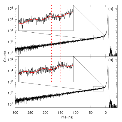
Figure 3: Time spectra for the 640-keV transition depopulating the $I^{\pi}=\frac{11}{2}^{-}$ isomer in ¹⁰⁷Cd. (a): Group $N_{1}$ defined in Eq. 2, (b): group $N_{2}$ defined in Eq. 3. Fits to guide the eye show the oscillations in the two groups out of phase. The prompt peak is due to a prompt 632-keV transition in ¹⁰⁶Cd which cannot be resolved from the 640-keV line by the LaBr₃ detectors.

Out-of-beam $\gamma$-ray energy spectra from HPGe and LaBr₃ detectors are shown in Fig. 2. Background-subtracted beam-$\gamma$ time spectra of the 640-keV transition are shown in Fig. 3. The fitted mean life of $\tau~{}=~{}101(2)$ ns agrees with previous measurements of $\tau=97(9)$ ns Hagemann et al. (1974) and $\tau~{}=~{}111(10)$ ns Bertschat et al. (1974a), and is within two standard deviations of the only other measurement, $\tau~{}=~{}107(3)$ ns Regan et al. (1995). The fit accounts for $\approx 20\%$ feeding from the higher $I^{\pi}=\frac{21}{2}^{+}$, $\tau=79(6)$ ns isomer in ¹⁰⁷Cd Hagemann et al. (1974); Regan et al. (1995). The amount of feeding was estimated from the HPGe energy spectrum, where the 520-keV transition can be resolved. If the feeding from the higher isomer is neglected, a value of $\tau=108(2)$ ns results. The treatment of feeding might explain the discrepancy between the present result and the lifetime reported in Ref. Regan et al. (1995).

The data were histogrammed in two groups to analyze the perturbed angular distribution. The first group comprised Detectors 1 ($+45^{\circ}$) and 3 ($-135^{\circ}$) when the field orientation was up, together with Detectors 2 ($+135^{\circ}$) and 4 ($-45^{\circ}$) when the field orientation was down. The second group was the converse: Detectors 2 and 4 for field up; and Detectors 1 and 3 for field down. Each detector within a group is affected by the precession of the angular distribution in the same way, whilst oscillations in the two groups should be 180^∘ out of phase. Figure 3 shows time spectra which display this behavior.

\begin{overpic}[width=216.81pt]{Fig2.pdf} \put(38.0,65.0){ \leavevmode\resizebox{128.0374pt}{}{ \sansmath \leavevmode\hbox to166.67pt{\vbox to106.44pt{\text{[drawing]}}} }} \end{overpic}

Figure 2: Out-of-beam $\gamma$-ray energy spectra recorded by (a) HPGe and (b) LaBr₃ detectors following reactions of 48-MeV ¹²C on ⁹⁸Mo. The inset in (b) shows the region around the 640-keV transition of interest and indicates the peak and background regions used to project the time spectra in Fig. 3.

III.1 Angular distributions

Angular distributions were measured using a HPGe detector. The anisotropy of the angular distribution depopulating the isomer cannot be measured directly because it loses its alignment during the long lifetime; however, decays of surrounding shorter-lived states give an indication of the initial anisotropy of the transition depopulating the isomer. Figure 4 shows the angular distributions of two of the transitions feeding the isomeric state. Both transitions have pure $E2$ multipolarity; the 956-keV is a transition between $I^{\pi}=\frac{23}{2}^{-}$ and $I^{\pi}=\frac{19}{2}^{-}$ states, whilst the 798-keV is between $I^{\pi}=\frac{19}{2}^{-}$ and $I^{\pi}=\frac{15}{2}^{-}$ states. The solid lines represent fits to the data with the spin alignment specified by a Gaussian distribution of width $\sigma$ Stuchbery and Robinson (2002); Diamond et al. (1966); Yamazaki (1967). The fit has two free parameters: $\sigma/I$ and a normalization factor. For the 798-keV and 956-keV transitions the fitted values are $\sigma/I=0.32(5)$ and $\sigma/I=0.30(6)$, respectively. A value of $\sigma/I\approx 0.3$ is common for heavy-ion fusion-evaporation reactions Stuchbery and Robinson (2002); Carpenter et al. (1990); Grau et al. (1974); Simms et al. (1974). The $\sigma/I$ parameter determines the anisotropy of the angular distribution depopulating the $I^{\pi}=\frac{11}{2}^{-}$ isomer, and has an impact on the amplitude of the $R(t)$ functions described in the following subsection.

Figure 4: Angular distribution of the (a) 798-keV and (b) 956-keV transitions in ¹⁰⁷Cd after population by the ⁹⁸Mo(¹²C, 3n) reaction. These stretched $E2$ transitions both feed the 846-keV isomer of interest and give a good indication of its spin alignment.

III.2 Ratio functions

A ratio function formed from the time spectra shows the precession of the angular distribution. The standard form for two detectors at $\pm 45^{\circ}$ to the beam-axis is

$$R(t)=\frac{N_{1}(t)-N_{2}(t)}{N_{1}(t)+N_{2}(t)}\approx\frac{3A_{2}}{4+A_{2}}\sin(2\omega_{L}t),$$ (1)

where $N_{1}(t)$ ($N_{2}(t)$) denotes the number of counts in the first (second) detector Recknagel (1974). The approximate expression applies when the unperturbed angular distribution can be written as $W(\theta)=1+A_{2}P_{2}(\cos(\theta))$, where $\theta$ is the angle with respect to the beam axis, $P_{2}$ is a second order Legendre polynomial, and $A_{2}$ is an orientation parameter Recknagel (1974); Witthuhn and Engel (1983). This form applies to our setup if we assign

$$N_{1}(t) =N(+45^{\circ})\uparrow+N(+135^{\circ})\downarrow$$ (2)

$$\qquad\qquad+N(-135^{\circ})\uparrow+N(-45^{\circ})\downarrow,$$

and

$$N_{2}(t) =N(+45^{\circ})\downarrow+N(+135^{\circ})\uparrow$$ (3)

$$\qquad\qquad+N(-135^{\circ})\downarrow+N(-45^{\circ})\uparrow,$$

where $N(\theta)\uparrow$ ($N(\theta)\downarrow$) denotes a detector at angle $\theta$ with respect to the beam axis with the field up (down). A modified definition is used to subtract background:

$$R(t)=\frac{T_{1}(t)-B_{1}(t)-T_{2}(t)+B_{2}(t)}{T_{1}(t)+T_{2}(t)-B_{1}(t)-B_{2}(t)},$$ (4)

where $T_{i}(t)$ represents the total peak area (without background subtraction) for the relevant group of detector/field direction combinations, and $B_{i}(t)$ is the area of the background region, multiplied by a scaling factor equal to the ratio of their widths (see Fig. 2(b) inset). In the present case, the background region shows no evidence of precession effects, and $B_{1}(t)\approx B_{2}(t)$, thus the form

$$R(t)=\frac{T_{1}(t)-T_{2}(t)}{T_{1}(t)+T_{2}(t)-B_{1}(t)-B_{2}(t)}$$ (5)

is used.

Figure 5: Ratio functions for ¹⁰⁷Cd in gadolinium. (a)-(d) correspond to data sets I-IV in Table 1 and in the text. Data sets are arranged in order of collection. The missing data near $t=0$ is on account of only using data well away from the (contaminant) prompt peak.

Ratio functions for a sequence of runs are shown in Fig. 5. Each function is formed from ${\sim}8$ hours of data collection. The ratio function has been fitted with the form

$$R(t)=Ce^{-\nicefrac{{t}}{{\kappa}}}\sin(2\omega_{L}t),$$ (6)

where the exponential term is phenomenological, and commonly used to account for decreasing alignment Mohanta et al. (2013); Mahnke (1989). Table 1 shows the fitted parameters for the relevant data sets.

Table 1: Fitted parameters for ratio functions.

Data Set	$\omega_{L}$ (Grad/s)	$\kappa$ (ns)	$C$
I	$-0.228(12)$	$18(4)$	$0.11(3)$
II	$-0.262(5)$	$30(4)$	$0.100(10)$
III	$-0.188(5)$	$31(8)$	$0.062(12)$
IV	$-0.209(8)$	$19(6)$	$0.07(2)$

IV Analysis of Ratio Functions

Two major features of the ratio functions shown in Fig. 5 are immediately apparent. First, the fitted amplitudes and frequencies vary significantly among data sets. The reasons for this observation will be discussed in Section IV.1.

Second, the amplitudes clearly attenuate rapidly, with no more than three or four periods visible. One possible explanation for this attenuation is that there are multiple oscillation frequencies present. If there were only two or three distinct frequencies (equivalent to the same number of field strengths), the frequency components would beat in and out of phase. There is no evidence of such behaviour occurring across the ${\sim}3$ mean lives observed, even using autocorrelation or Fourier-transform analysis. Thus a near continuous distribution of fields is implied. This conclusion will be discussed, and alternative explanations of the observed $R(t)$ data will be explored, in Sections IV.2 and IV.3.

IV.1 Accumulating Radiation Damage

Both the initial amplitude ($C$) and the frequency ($\omega_{L}$) of the $R(t)$ data changed on macroscopic time scales. As well as being determined by the anisotropy of the unperturbed angular distribution, $C$ is dependent on the proportion of nuclei that are implanted into field-free sites, $f$. When $f$ is high, many nuclei decay without undergoing precession, reducing the amplitude of the ratio function.

Data sets gathered later in the experiment show a decrease in both $\omega_{L}$ and $C$, which can be attributed to accumulating radiation damage to the gadolinium host. Thus, to relate the present observations to the previous measurement of $g(10^{+})$ in ¹¹⁰Cd, it is important to match the level of accumulated beam dose. The present work used beam intensities up to an order of magnitude higher than those in the previous ¹¹⁰Cd $g$-factor measurement Regan et al. (1995). As a consequence, the equivalent cumulative dose to the gadolinium host was reached before the end of data set II (see Fig. 5 and Table 1). For this reason we use only data sets I and II to re-evaluate $g(10^{+})$ in ¹¹⁰Cd in Section V below.

IV.2 Electric Field Gradients

Along with the magnetic dipole interaction, the electric quadrupole interaction associated with an electric field gradient (EFG) must be considered in the case of a gadolinium host. The hexagonal close-packed (hcp) crystal structure means that the quadrupole interactions do not cancel Witthuhn and Engel (1983). The frequency ($\omega_{Q}$) associated with the EFG is given by

$$\omega_{Q}=\frac{eQ}{4I(2I-1)\hbar}V_{zz},$$ (7)

where $Q$ and $I$ are the electric quadrupole moment and angular momentum of the nuclear state respectively, and $V_{zz}$ is the $z$-component of the EFG Witthuhn and Engel (1983).

The combined electric-magnetic interaction has been examined thoroughly for the $I^{\pi}=\frac{5}{2}_{1}^{+}$ state of ¹¹¹Cd in gadolinium by studying the $\gamma$-$\gamma$ angular correlations after ¹¹¹In decay Bostrom et al. (1971); Forker and Hammesfahr (1973); de la Presa et al. (2004). Each of these experiments used an amorphous sample with no polarizing field. Thus the EFG and $B_{\rm hf}$ are randomly oriented; however, there is a preferred angle ($\beta$) between $V_{zz}$ and $B_{\rm hf}$ for any individual gadolinium microcrystal Boström et al. (1970); Forker and Hammesfahr (1973); Bostrom et al. (1971); de la Presa et al. (2004). In such experiments, the time-dependent angular correlation function can be expressed as

$$W(\theta,t)=1+A_{22}G_{22}(t)P_{2}(\cos\theta),$$ (8)

where the $A_{22}$ coefficient is the $\gamma$-$\gamma$ angular correlation equivalent of the $A_{2}$ discussed in Section III.2; the $A_{44}$ term is neglected Frauenfelder and Steffen (1966). These experiments measured the perturbation factor $G_{22}(t)$ to obtain the angle $\beta$, electric quadrupole frequency $\omega_{Q}$, and magnetic dipole frequency $\omega_{L}$. It should be noted that $G_{22}(t)$ and $R(t)$ are fundamentally different observables that apply to different experimental setups, although they reflect the same physical phenomena. A direct comparison between the $G_{22}(t)$ functions obtained in the off-line measurements, (Refs. Bostrom et al. (1971); Forker and Hammesfahr (1973); de la Presa et al. (2004)), and $R(t)$ of the present measurements that apply a polarizing field, is not meaningful. However, $G_{22}(t)$ and the corresponding $R(t)$ applicable to our experiment resulting from the combined electric-magnetic interaction can be evaluated. Examples of calculations for ¹¹¹Cd and ¹⁰⁷Cd in gadolinium are shown in Fig. 6 and Fig. 7, respectively. The $G_{22}(t)$ calculations assume a polycrystaline source with no external field applied, as in Refs. Bostrom et al. (1971); Forker and Hammesfahr (1973); de la Presa et al. (2004). The calculated $R(t)$ functions, however, have an external polarizing magnetic field applied perpendicular to the plane of the detectors as in the present experimental setup.

Figure 6 shows a simulation of $G_{22}(t)$ and $R(t)$ from the combined magnetic and electric interactions for the $I^{\pi}=\frac{5}{2}^{+}$ state in ¹¹¹Cd ($E_{x}=254$ keV, $\tau~{}=~{}121.9$ ns) in gadolinium. A conservative estimate of $V_{zz}~{}=~{}1.4~{}\times~{}10^{17}$ V/cm² is used, with $B_{\rm hf}=-34$ T, $\beta=30^{\circ}$ de la Presa et al. (2004), $Q=0.77$ Raghavan et al. (1973), and $g=-0.306$ Bertschat et al. (1974b). The calculated $G_{22}(t)$ matches that shown in Fig. 1 of Ref. de la Presa et al. (2004). Note that the ratio function for the same parameters shows very different behavior: the attenuation due to the electric quadrupole interaction is slower because the magnetic interaction is held in the direction of the polarizing field.

Similarly, Fig. 7 shows both $G_{22}(t)$ and $R(t)$ for the $E_{x}=846$ keV, $I^{\pi}=\frac{11}{2}^{-}$ state of ¹⁰⁷Cd in gadolinium. The same $B_{\rm hf}$ and $V_{zz}$ are used, with $Q=0.94$ Sprouse et al. (1978) and $g=-0.189$ Raghavan (1989). Apart from the change in Larmor frequency due to the change in $g$ factor, the striking difference in $G_{22}(t)$ compared to Fig. 6 stems from the change in nuclear spin. It is clear from Fig. 7(b) that the electric quadrupole interaction is not nearly strong enough to explain the decay of the ratio function as displayed by the experimental data in Fig. 5. In terms of the effective decay constant, $\kappa$, the experimental data show $\kappa\approx 18\text{--}30$ ns (Table 1), whereas the evaluation of the effect of the EFG in Fig. 7 implies $\kappa\approx 114$ ns. It should be noted that the calculations are conservative (maximizing the electric quadrupole interaction): $V_{zz}=1.4\times 10^{17}$ V/cm² was reported in Ref. de la Presa et al. (2004), whereas two other measurements report smaller electric field gradients, $V_{zz}=0.85\times 10^{17}$ V/cm² Forker and Hammesfahr (1973) and $V_{zz}=0.21\times 10^{17}$ V/cm² Bostrom et al. (1971). Also, in the case of our experimental geometry it is highly likely the $c$-axis of the hexagonal close packed structure (and so the EFG direction) is perpendicular to the foil and hence parallel to the beam direction. This is a known property of cold-rolled and annealed gadolinium foils, which has been observed in X-ray diffraction measurements and confirmed by magnetization versus temperature curves Stuchbery et al. (2006); Robinson et al. (1999). With the $c$ axis along the beam direction, $\beta=90^{\circ}$ and the effect of the EFG on the ratio function is reduced.

In summary, it is evident that the effect of the EFG is not nearly significant enough to account for the attenuation in the observed $R(t)$ functions, and that EFG effects can be neglected in further analysis.

Figure 6: Simulation of (a) $G_{22}(t)$ and (b) $R(t)$ from combined magnetic and electric interactions for the $I^{\pi}=\frac{5}{2}^{+}$ state in ¹¹¹Cd ($E_{x}=254$ keV, $\tau=121.9$ ns) in gadolinium. If the form of Eq. 6 is assumed for $R(t)$, $\kappa\approx 61$ ns. The $G_{22}(t)$ function corresponds to a polycrystalline source with no external field, whilst the $R(t)$ function is applicable to the present experiment with a polarizing external field at $90^{\circ}$ to the plane of detection.

Figure 7: A simulation analogous to Fig. 6, showing (a) $G_{22}(t)$ and (b) $R(t)$ for the $E_{x}=846$ keV, $I^{\pi}=\frac{11}{2}^{-}$ ¹⁰⁷Cd state in gadolinium. The solid line is for $\beta=30^{\circ}$, and the dashed for $\beta=90^{\circ}$. If the form of Eq. 6 is assumed for $R(t)$, $\kappa\approx 114$ ns. See also Fig. 6 caption.

IV.3 Distribution of field strengths

Another explanation for the attenuation of the ratio function is that a continuous distribution of field strengths is present across a range of implantation sites instead of a single, well-defined $B_{\rm hf}$. A ratio function can be calculated using the angular distributions measured to set the initial anisotropy, assuming alternative distributions of field-strengths, and a field-free fraction $f$. The distribution parameters, such as the width and average value, can then be fitted to the experimental data. The calculated ratio functions were also attenuated to $0.87$ of the full amplitude to account for the convolution of the beam pulse and time resolution of the LaBr₃ detectors (${\sim}2$ ns) with the $R(t)$ function. This factor was calculated by evaluating the convolution of a sinusoid of an appropriate frequency with a Gaussian with FWHM of $2$ ns. The factor is not sensitive to small changes in the frequency.

A Gaussian distribution of hyperfine fields was found to reproduce the observed $R(t)$ data, however as shown in Fig. 8 and Table 2, the ratio function is not sensitive to the precise shape of the field distribution. As evident from Fig. 8 and the fit parameters in Table 2, fits of equal quality were obtained with Gaussian, Lorentzian, and Half-Gaussian field distributions for data set II (reduced $\chi^{2}=0.99,0.99,$ and $1.00$, respectively). Along with the shape of the field distribution, the fraction of nuclei on field-free sites ($f$) was also fitted. For convenience, Gaussian field distributions were adopted for the re-analysis of the ¹¹⁰Cd $g(10^{+})$ measurement which follows.

Table 2: Field distribution parameters from fitting the ¹⁰⁷Cd ratio function data (Fig. 5) in the process described in Section IV.3. $\Delta B_{\rm hf}$ is the FWHM of the distribution.

Data Set	$\overline{B_{\rm hf}}$ (T)	$\Delta B_{\rm hf}$ (T)	Distribution	$f$
p I	$-24.3(4)$	$6.6(8)$	Gaussian	$0.54(5)$
II	$-29.0(2)$	$4.7(4)$	Gaussian	$0.53(3)$
II	$-29.0(2)$	$3.6(3)$	Lorentzian	$0.45(3)$
II	$-27.8(2)$	$4.2(3)$	Half-Gaussian	$0.52(3)$
III	$-20.7(3)$	$4.4(5)$	Gaussian	$0.72(3)$
IV	$-22.9(4)$	$6.6(8)$	Gaussian	$0.70(4)$

Figure 8: Ratio functions from different field distributions: red solid line, Gaussian; blue dashed line, Half-Gaussian; green dashed-dotted line, Lorentzian. (a): Fits of the ratio functions to data set II. (b): Field distributions, parameters specified in rows two to four in Table 2.

V Correcting the $\bm{g(10^{+})}$ measurement

The field-free fraction plays a dominant role in determining the effective hyperfine-field strength for integral precession measurements like the $g(10^{+})$ measurement in ¹¹⁰Cd of Ref. Regan et al. (1995). The usual expression for the integral perturbed angular distribution in the case where there is a unique field and hence unique Larmor frequency $\omega$, is:

$$W(\theta)=\sum_{k}\frac{b_{k}}{\sqrt{1+(k\omega\tau)^{2}}}\cos(k[\theta-\Delta\theta_{k}]),$$ (9)

where $\Delta\theta_{k}$ are the solutions of $\tan(k\Delta\theta_{k})=k\omega\tau$, and the $b_{k}$ coefficients ($k=0,2,4)$ are related to the $A_{k}$ orientation parameters as given in Refs. Recknagel (1974); Regan et al. (1995). With a distribution of fields, the expression becomes

$$W(\theta)=\sum_{ki}\frac{p_{i}b_{k}}{\sqrt{1+(k\omega_{i}\tau)^{2}}}\cos(k[\theta-\Delta\theta_{ki}]),$$ (10)

where $\tan(k\Delta\theta_{ki})=k\omega_{i}\tau$, and $p_{i}$ is the fraction of nuclei implanted into a site with field $B_{i}$, causing a precession at Larmor frequency $\omega_{i}$.

Equation 10 can be fitted to the original perturbed angular distribution data from Ref. Regan et al. (1995), using the field distribution, including the field-free fraction, taken from the present ¹⁰⁷Cd measurement. A value of $\tau=700(30)$ ps has been adopted for the mean life of the $I^{\pi}=10^{+}$ state in ¹¹⁰Cd Kostov et al. (1998); Juutinen et al. (1994); Piiparinen et al. (1993); Harissopulos et al. (2001). The distributions found in data sets I and II (parameters on the first two rows of Table 2) were used separately and together. If the distribution formed by taking the weighted average of the parameters from data sets I and II is used, $g(10^{+})=-0.29(16)$ is found from the resultant fit shown in Fig. 9. To assess the changes in effective field strength on a macroscopic time scale, the $g$ factor was also evaluated based only on data set I, giving $g(10^{+})=-0.34$, and data set II alone giving $g(10^{+})=-0.28$, a difference of only 0.06 compared to the 0.16 uncertainty in the weighted average. These results show that the statistical error from the original perturbed angular distribution measurement is much more significant than the uncertainty from the variation in fields between data sets I and II.

Figure 9: Fits to perturbed angular distribution data from Ref. Regan et al. (1995). A field distribution formed by taking a weighted average of the parameters extracted from data sets I and II was used (see the first two rows of Table 2). The $g$ factor was varied to obtain the best fit. The blue solid line is the perturbed angular distribution fit, the dotted red line is the unperturbed angular distribution.

It is worth noting that the decay of the ratio function is of little importance for the interpretation of the integral $g$-factor measurement because the precession in the integral measurement takes place in only the first few nanoseconds. The most significant impact on the $g$-factor evaluation originated from the fraction of nuclei implanted onto field-free sites.

In summary, we adopt the weighted average of data sets I and II to fit to the perturbed angular distribution data from Ref. Regan et al. (1995). The result is $g(10^{+})=-0.29(16)$. For a $\nu(h_{\nicefrac{{11}}{{2}}})^{2}$ configuration the Schmidt value is $g=-0.348$, or with quenching of the spin $g$ factor to 70% of the free nucleon value, $g=-0.243$. Thus the experimental value is consistent with the $(h_{\nicefrac{{11}}{{2}}})^{2}$ neutron description of the state Castel and Towner (1990); Bohr and Mottelson (1969); Frömmgen et al. (2015); Yordanov et al. (2013).

VI Discussion

VI.1 Comparison with previous work

An in-beam time differential measurement of the hyperfine fields of Cd in gadolinium has been reported here for the first time. The frequencies observed in Fig. 5 imply hyperfine fields close to, but slightly less than, what is expected from offline measurements on Cd in gadolinium Krane (1983); Forker and Hammesfahr (1973). However, the ratio functions observed in-beam attenuate more rapidly than expected based on the off-line data. This strong attenuation is attributed to an effectively continuous distribution of hyperfine field values on the implantation sites. The width of the field-strength distribution is significantly larger than that reported by previous offline observations of hyperfine fields for Cd in gadolinium Forker and Hammesfahr (1973). However, the distribution widths (as a fraction of average field strength) observed are comparable with previous in-beam measurements on Ga, Ge, and As implanted into gadolinium: between about $5\%$ and $18\%$ Raghavan et al. (1979); Raghavan and Raghavan (1985).

VI.2 Implications for other measurements

The fraction of nuclei in field-free sites was significant. The consequence is that the effective hyperfine field for in-beam integral Perturbed Angular Correlation/Distriubtion measurements of Cd in gadolinium is much reduced compared to offline measurements. Extracting the field-free fraction precisely proved difficult as the dependence of the initial amplitude of the ratio function on the width and shape of the field-strength distribution makes the quantitative analysis complex and multiplies uncertainties.

The precession frequency was also observed to vary on macroscopic time scales. This variation can only be attributed to a change in the hyperfine field strength. The timing electronics were proven to be stable because the mean-life measurements on subsets of the data were consistent throughout the experiment. The changes in field-strength are most likely due to the accumulation of radiation damage. In the case where the field strength increased, we assume that the beam spot moved to an undamaged or less damaged location on the target, resulting in a temporary return to a higher average hyperfine-field strength.

The observation that the later data sets have a much higher field-free fraction is consistent with the suggestion that increasing accumulated radiation damage is responsible. Unfortunately it was difficult to replicate the accumulated radiation dose of the $g(10^{+})$ measurement precisely. However, the difference in effective fields and deduced $g$ factors for data sets I and II is small compared to the uncertainties for the perturbed angular distribution data from the integral $g$-factor measurement. Thus, despite the uncertainties in the evaluation of the effective hyperfine field strength, it is now clear that the experimental $g(10^{+})$ value is consistent with that of the expected seniority-two $\nu h_{\nicefrac{{11}}{{2}}}$ configuration. A more extensive $g$-factor experiment might involve measuring both the time-integral ¹¹⁰Cd and the time-differential ¹⁰⁷Cd simultaneously, with a low beam current to avoid accumulating radiation damage. However, such experimental conditions are not easily implemented. An alternative host, which does not accumulate radiation damage so severely, should be sought for future experiments. For example, it would be worthwhile to explore the behaviour of Cd ions implanted into iron hosts. Previous experiments implanting Ge into iron show no loss of alignment over more than ${\sim}500$ ns Raghavan et al. (1979); Raghavan and Raghavan (1985), in contrast to implantation into gadolinium where the alignment is lost within ${\sim}100$ ns Lee (1988); Lee et al. (1991).

VII Conclusion

LaBr₃ detectors have been applied to the in-beam TDPAD technique and their effectiveness has been demonstrated by the measurement of a frequency that proved too fast to resolve with HPGe detectors. Future applications of LaBr₃ detectors to measure precessions with periods of ${\sim}5$ ns in-beam are feasible.

There are, however, unanswered questions about gadolinium as a ferromagnetic host for in-beam $g$-factor measurements of this type. Whether the behavior observed here (significant distribution of fields, variation of field strength on macroscopic time scales) is typical of gadolinium as a host in general, or specific to the case of Cd in gadolinium studied here, remains to be investigated more thoroughly.

Despite these uncertainties, it is clear that the previous $g(10^{+})$ measurement in ¹¹⁰Cd was based on an incorrect value for the effective hyperfine field. With the field corrected from the present study, the $g$ factor becomes consistent with the theoretical understanding that the $I^{\pi}=10^{+}$ state is associated with a seniority-two $\nu h_{\nicefrac{{11}}{{2}}}$ configuration. This example demonstrates the value of time-differential techniques as a complimentary tool to validate or calibrate time-integral $g$-factor measurements.