Distributed Join-the-Idle-Queue for Low Latency Cloud Services

Abstract

Low latency is highly desirable for cloud services. To achieve low response time, stringent timing requirements are needed for task scheduling in a large-scale server farm spanning thousands of servers. In this paper, we conduct an in-depth analysis for distributed Join-the-Idle-Queue (JIQ), a promising new approximation of an idealized task-scheduling algorithm. In particular, we derive semi-closed form expressions for the delay performance of distributed JIQ, and we propose a new variant of distributed JIQ that offers clear advantages over alternative algorithms for large systems.

I INTRODUCTION

I-A Motivation

In cloud communication, low latency is highly desirable for online services spanning thousands of servers. For example, Google search typically returns the query results within a few hundreds of milliseconds. According to Google and Amazon, an extra latency of $500$ milliseconds in response time could result in a $1.2\%$ loss of users and revenue [1]. The demand for fast response time, which significantly impacts user experience and service-provider revenue, is translated into stringent timing requirements for task scheduling in a large-scale server farm.

Join-the-Shortest-Queue (JSQ) is an idealized algorithm to achieve short response time. It tracks the queue lengths of all the servers and selects the least loaded server for a newly arrival task. Although JSQ is proven to be latency optimal [2], it doesn’t scale well as the system size increases. The reason is that tracking the global queue-length information is both time and resource consuming. To alleviate this problem, the Power-of-$d$-Choices (Po$d$) algorithm ($d\geq 2$) has been proposed as an “approximation" of the idealized JSQ. Instead of tracking the global information, Po$d$ only probes $d$ servers uniformly at random upon a task arrival and selects the least loaded one for the new task. Although Po$d$ achieves reasonably good average response time [3], its tail response time still remains high for large-scale systems [4, 5] and its probing operation incurs additional delay.

Recently, distributed Join-the-Idle-Queue (JIQ) [6] has emerged as a promising new approximation of JSQ. JIQ employs a number of distributed schedulers, each maintaining an I-queue that stores a list of idle servers. When a new task arrives at the system, it randomly visits a scheduler, asking to join an idle server in its I-queue. Compared to JSQ, each scheduler in JIQ only maintains local information and is scalable to large systems. Compared to Po$d$, each scheduler in JIQ avoids the probing operation and assigns a new task to an idle server directly as long as its I-queue is non-empty. Due to its clear advantages, JIQ has begun to attract research attention from both industry and academia [7, 8, 9, 10]. Despite these significant research achievements made recently, distributed JIQ is not yet well understood from a theoretical perspective. For example, there is no closed-form expression yet that exactly characterizes the delay performance of distributed JIQ [7]. Also, there seems no theoretical guarantee that the distributed JIQ (or any of its variants) is strictly better than Po$d$.

I-B Contributions

In this paper, we take a further step in understanding the performance of distributed JIQ. As our first contribution, we apply a mean-field analysis to derive semi-closed form expressions of the stationary tail distribution and the expected response time for distributed JIQ. Our expressions contain a parameter $\hat{p}_{0}\in(0,1)$ that can be efficiently calculated by a binary search. We show that, in the large-system limit, the tail probability $\hat{s}_{i}$ of a server having at least $i$ tasks is given by $\hat{s}_{i}=\hat{p}_{0}^{i-1}\lambda^{i}$, where $\lambda$ is the normalized arrival rate. We also show that the expected task response time is $1+\hat{p}_{0}\sum_{i=1}^{\infty}\hat{s}_{i}$. These two expressions allow us to compare JIQ and Po$d$ directly and find that JIQ is not always better than Po$d$.

As our second contribution, we propose a new variant of JIQ called JIQ-Po$d$ that strictly outperforms Po$d$. JIQ-Po$d$ enjoys the best of both worlds. Similar to JIQ, a scheduler with a non-empty I-queue in JIQ-Po$d$ assigns a new task to an idle server on its I-queue. Similar to Po$d$, a scheduler with an empty I-queue in JIQ-Po$d$ probes $d$ servers and selects the least loaded one. Intuitively, JIQ-Po$d$ improves upon JIQ in that it makes schedulers with empty I-queues “smarter"; it improves upon Po$d$ in that schedulers with non-empty I-queues can assign new tasks directly to idle servers without the probing operation. Using the mean-field analysis, we are able to quantify the improvements of JIQ-Po$d$ over JIQ and Po$d$ in the large-system limit.

I-C Related Work

The Po$d$ algorithm and its variants have been widely studied and applied in today’s cloud systems. One variant is called batch filling [5], which is designed for batch arrivals. It achieves lower tail response time than the Po$d$ algorithm and guarantees a bounded maximum queue-length for the system. Another variant is a hybrid algorithm that combines the Po$d$ with a centralized helper [11]. In particular, such hybrid algorithm achieves a bounded maximum queue-length and lower response time even when the helper has a small portion of processing capacity. Unlike these variants, JIQ and JIQ-Po$d$ neither rely on batch arrivals nor rely on a centralized helper.

The JIQ algorithm was originally proposed in a seminal work [6] in 2011. The authors assumed that all servers in I-queues are idle as a simplification of their performance analysis. As pointed out in [6], this assumption is violated when an idle server receives a random arrival. In this work, we do not make such assumption. Instead, we introduce delete request messages (as explained later) to ensure that all servers in I-queue are idle.

Recently, Mitzenmacher studied the distributed JIQ algorithm through a fluid-limit approach [7]. He proposed an elegant classification of the states of servers and derived families of differential equations that describe the JIQ system in the large-system limit. Due to the high complexity of those differential equations, there is no expression of the equilibrium in a convenient form in terms of $\lambda$ [7]. Our work is inspired by Mitzenmacher’s fluid-limit approach. By introducing delete request messages, we are able to simplify the differential equations and obtain semi-closed form expressions for distributed JIQ. Based on the insights from our analysis, we propose and analyzed a new variant of JIQ that outperforms both JIQ and Po$d$ in all conditions.

In a series of papers [8, 9, 10], Stolyar studied a centralized JIQ algorithm where there is only one scheduler (or a fixed number of schedulers) in the system through mean-field analysis. It shows that centralized JIQ approaches the performance of JSQ in the large-systems limit. This exciting result means that a centralized scheduler only needs to track idle servers instead of all the servers. Our work is complementary to Stolyar’s work in that we focus on distributed JIQ rather than cetralized JIQ.

Also, several recent studies explored the tradeoff between the communication overheads and the task/job response times  [12, 13] as well as the tradeoff between the energy consumption and the task/job response times  [14] for JIQ-like algorithms. The techniques developed in this work might be useful to these studies as well.

I-D Organization of the Paper

Section II introduces our system model and main results. In Section III, we perform the mean-field analysis for both JIQ and JIQ-Po$d$. In Section IV, extensive simulations are conducted to validate our analysis. Finally, Section V concludes the paper.

II System Model and Main Results

In this section, we will introduce the system model of the distributed JIQ algorithm as well as a new variant—distributed JIQ-Po$d$ algorithm. We will then compare these two algorithms with the Po$d$ algorithm in terms of tail distribution of servers and expected task response time.

II-A Distributed JIQ Algorithm

Consider a system with $N$ identical servers and $M$ schedulers, where the ratio $r$ is defined as $r=N/M$. Each scheduler is equipped with an I-queue that stores a list of idle servers (which will be specified later).

TABLE I: summary of queue length distribution under JIQ, JIQ-Po$d$ and Po$d$.

	JIQ	JIQ-Po$d$	Po$d$
Tail distribution of server ($\hat{s}_{i}$ for $i\geq 1$)	$\hat{p}_{0}^{i-1}{\lambda^{i}}$	${\lambda^{\frac{{{d^{i}}-1}}{{d-1}}}}\hat{p}_{0}^{\frac{{{d^{i-1}}-1}}{{d-1}}}$	${\lambda^{\frac{{{d^{i}}-1}}{{d-1}}}}$
Expected task response time ($T(\lambda)$)	$1+{\hat{p}_{0}}\sum\limits_{i=1}^{\infty}{{{{\hat{s}_{i}}}}}$	$1+{\hat{p}_{0}}\sum\limits_{i=1}^{\infty}{{{({\hat{s}_{i}})}^{d}}}$	$1+\sum\limits_{i=1}^{\infty}{{{({\hat{s}_{i}})}^{d}}}$

The system evolves as follows:

• Task arrivals: Tasks arrive at the system according to a Poisson process of rate $\lambda N$, where $\lambda<1$, and are sent to a scheduler uniformly at random. Thus, each scheduler observes a Poisson arrival process of rate $\lambda N/M$.

• Schedulers with I-queues: Each scheduler has an I-queue, which maintains a list of idle servers. Upon a task arrival, each scheduler checks its I-queue and assigns the task to a server according to the following rule: If the I-queue is non-empty, the scheduler selects an idle server uniformly at random from its I-queue. If the I-queue is empty, the scheduler selects a server uniformly at random from all the servers.

• Servers: Each server has an infinite buffer and processes tasks in a first-in first-out (FIFO) manner. The task processing times are exponentially distributed with mean $1$. Whenever a server becomes idle, it joins an I-queue selected uniformly at random among all I-queues. Whenever an idle server becomes busy, it leaves its associated I-queue in one of the following two ways:

  

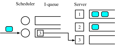
  Figure 1: Server $3$ is selected by Scheduler $2$ and leaves its I-queue, where 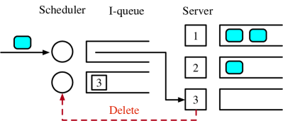$N=3$ and $M=2$.

  

  Figure 2: Server $3$ is selected by Scheduler $1$ and sends a “delete request” message to Scheduler $2$, where $N=3$ and $M=2$.

  1. If it is selected by a scheduler with a non-empty I-queue, then it simply leaves the I-queue, as shown in Figure 1.

  2. If it is selected by a scheduler with an empty I-queue, then it has to inform its associated I-queue by sending a “delete request” message, as shown in Figure 2.

Remark 1:

We note that some distributed JIQ algorithm doesn’t use the “delete request” messages (e.g., in [7]), allowing I-queues having non-idle servers. Although it reduces the communication overhead, it complicates the theoretical analysis. As we will see in Section IV-B, such extra communication overhead is acceptable.

II-B Distributed JIQ-Po$d$ Algorithm

The distributed JIQ algorithm described above doesn’t always outperform the Po$d$ algorithm, especially under heavy workload where most I-queues are empty. To address this issue, we propose a new variant of JIQ, namely JIQ-Po$d$, which combines the advantages of JIQ and Po$d$. It works as follows.

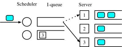
Schedulers under JIQ-Po$d$. Upon a task arrival, each scheduler checks its I-queue and assigns the task to a server according to the following rule: If its I-queue is non-empty, the scheduler selects an idle server uniformly at random from its I-queue. If its I-queue is empty, the scheduler probes $d$ servers uniformly at random and assigns the task to the least loaded one, as shown in Figure 3. Essentially, each scheduler with an empty I-queue is applying the Po$d$ strategy.

All other steps remain the same as the distributed JIQ algorithm. Clearly, when $d=1$, our JIQ-Po$d$ algorithm reduces to the distributed JIQ.

Figure 3: Scheduler $1$ probes Server $1$ and Server $3$, and assigns a new task to Server $3$, where $N=3$ and $M=2$.

II-C Main Results

Table I presents our main results that characterize the stationary tail distribution and the expected task response time in the large-system limit (i.e., $N\rightarrow\infty$ and $M\rightarrow\infty$ with the ratio $r=N/M$ fixed), where $\hat{p}_{0}$ is some parameter in $(0,1)$ (which will be specified later). The stationary tail distribution $\hat{s}_{i}$ is the fraction of servers having no less than $i$ tasks in their task queues. (Note that $\hat{s}_{0}$ is always equal to $1$, and that the $\{\hat{s}_{i}\}$ are non-increasing.) The smaller $\hat{s}_{i}$ is, the shorter the task delay. The expected task response time $T(\lambda)$ measures the average completion time for a task in steady state.

First, we observe that JIQ-Po$d$ gives the best tail distribution $\hat{s}_{i}$. Compared to Po$d$, JIQ-Po$d$ has an additional factor of ${\hat{p}_{0}^{\frac{{{d^{i-1}}-1}}{{d-1}}}}<1$, since $\hat{p}_{0}\in(0,1)$. For instance, when $d=2$, $i=2$ and $p_{0}=0.5$, such factor equals to $0.5$. Compared to JIQ, JIQ-Po$d$ has larger exponents of $\lambda$ and $\hat{p}_{0}$. For example, when $d=2$ and $i=3$, the exponent of $\lambda$ under JIQ-Po$d$ is ${\frac{{{d^{i}}-1}}{{d-1}}}=7>i=3$, and the exponent of $\hat{p}_{0}$ under JIQ-Po$d$ is ${\frac{{{d^{i-1}}-1}}{{d-1}}}=3>i-1=2$.

Figure 4: Comparison of the expected task response time among JIQ, JIQ-Po$d$ and Po$d$, when $r=10$ and $d=2$.

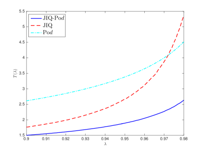
Second, we observe that JIQ-Po$d$ achieves the shortest expected task response time $T(\lambda)$. Compared to Po$d$, JIQ-Po$d$ has an additional factor of $\hat{p}_{0}<1$. Compared to JIQ, JIQ-Po$d$ has larger exponents of $\hat{s}_{i}$. To better illustrate the advantage of JIQ-Po$d$, we provide a concrete numerical example in Figure 4, which shows that, when $\lambda=0.98$, $T(\lambda)$ of JIQ-Po$d$ is only around $2.6$, whereas $T(\lambda)$ of JIQ and Po$d$ are $5.3$ and $4.5$, respectively.

III Mean-Field Analysis

In this section, we will use the mean-field analysis to study the stationary distributions of the queue lengths, as well as the corresponding expected task response time, under JIQ. We will then apply the same analysis to JIQ-Po$d$. The underlying assumptions behind the mean-field analysis will be validated through simulations in Sec. IV-A. In fact, these assumptions can be rigorously validated using proof techniques such as Kurtz’s theorem, which is beyond the scope of this paper.

First, we look at the state of a single server in the system. Let $\left(X_{i}^{(N)}(t),Y_{i}^{(N)}(t)\right)$ denote the state of the $i$th server at time $t$ in a system of $N$ servers and $M$ I-queues, where $X_{i}^{(N)}(t)$ is the queue length of the $i$th server at time $t$ and $Y_{i}^{(N)}(t)$ is the index of the associated I-queue. If the $i$th server doesn’t belong to any I-queue at time $t$, we set $Y_{i}^{(N)}(t)=0$. It is easy to check that $\left\{\left(X_{i}^{(N)}(t),Y_{i}^{(N)}(t)\right)\right\}_{i=1}^{N}$ forms an irreducible, aperiodic, continuous-time Markov chain under our system model. Moreover, the following theorem shows that this Markov chain is positive recurrent. Thus, it has a unique stationary distribution.

Theorem 1:

The Markov Chain $\left\{\left(X_{i}^{(N)}(t),Y_{i}^{(N)}(t)\right)\right\}_{i=1}^{N}$ under the JIQ algorithm is positive recurrent.

Proof:

We first construct a potential function and then apply Foster-Lyapunov theorem. Please see Appendix -A for details. ∎

We now introduce a new representation of the system state to conduct the mean-field analysis. Let $Q_{i}^{(N)}(t)$ denote the number of servers with $i$ tasks at time $t$. Let $Q_{(0,j)}^{(N)}(t)$ denote the number of idle servers that belong to I-queues of size $j$ at time $t$. Then, the system state at time $t$ can be described by

$${{\mathbf{Q}}^{(N)}}(t)=\left\{{Q_{(0,1)}^{(N)}(t),Q_{(0,2)}^{(N)}(t),\cdots,Q_{1}^{(N)}(t),Q_{2}^{(N)}(t),\cdots}\right\}.$$

One can verify that ${{\mathbf{Q}}^{(N)}}(t)$ also forms a continuous-time Markov chain under our system model, because the individual servers (or I-queues) of the same queue-length are indistinguishable for system evolution. In other words, our new Markov chain ${{\mathbf{Q}}^{(N)}}(t)$ captures the “essential" information of our original Markov chain $\left\{\left(X_{i}^{(N)}(t),Y_{i}^{(N)}(t)\right)\right\}_{i=1}^{N}$. In particular, if our original Markov chain has a unique stationary distribution, so does our new Markov chain.

For convenience, we further introduce a normalized version of ${{\mathbf{Q}}^{(N)}}(t)$ defined as

$${\widetilde{\mathbf{Q}}^{(N)}}(t)=\frac{1}{N}{{\mathbf{Q}}^{(N)}}(t).$$

Note that $\tilde{Q}_{(0,j)}^{(N)}(t)$ is the fraction of servers that belong to I-queues of size $j$ at time $t$, and $\tilde{Q}_{i}^{(N)}(t)$ is the fraction of servers with $i$ tasks at time $t$. Clearly, ${\widetilde{\mathbf{Q}}^{(N)}}(t)$ is also positive recurrent and has a unique stationary distribution. In addition, we can show that ${\widetilde{\mathbf{Q}}^{(N)}}(t)$ is density dependent.

The mean-field analysis proceeds as follows. We assume that the $N$ servers are in the steady state. We also assume that the states of these servers are identically and independently distributed (i.i.d.) [5]. This i.i.d. assumption will be validated later through simulations. We now consider the state evolution of one server in the system under the i.i.d. assumption. Note that the possible server states are from the set

$$\{(0,1),(0,2),\ldots,1,2,\ldots\}$$

where the state-$(0,j)$ means that the server is idle and belongs to an I-queue of size $j$, and the state-$i$ means that the server has $i$ tasks in its queue. Let

$${\mathbf{q}}=\left\{{{q_{(0,1)}},{q_{(0,2)}},\cdots,{q_{1}},{q_{2}},\cdots}\right\}$$

denote the stationary distribution of the server state. (Note that ${\mathbf{q}}$ is unique because ${\widetilde{\mathbf{Q}}^{(N)}}(t)$ is positive recurrent.) Then, by the Strong Law of Large Numbers, $q_{0,j}$ can be interpreted as the fraction of servers belonging to an I-queue of size $j$, and $q_{i}$ can be interpreted as the fraction of servers with $i$ tasks in the large-system limit. This means that the stationary distribution of ${\widetilde{\mathbf{Q}}^{(N)}}(t)$ “concentrates" on ${\mathbf{q}}$ as $N\to\infty$.

We are now ready to derive the stationary distributions under JIQ and JIQ-Po$d$ in the large-system limit.

III-A The Stationary Distribution Under JIQ

In this subsection, we will derive the stationary distribution of one server in the system under JIQ. The i.i.d. assumption described above allows us to obtain the transition rates for the state evolution of the server. In fact, this assumption holds asymptotically in the large-system limit. In other words, the stationary distribution derived here is sufficiently accurate for large-scale systems.

To derive the transition rates, we need some additional notations. Let $p_{i}$ be the fraction of I-queues of size $i$ in the large-system limit. Then we have

$$p_{i}=\left\{\begin{array}[]{ll}\frac{{r{q_{(0,i)}}}}{i},&i\geq 1,\\ 1-\sum\limits_{j=1}^{\infty}\frac{{r{q_{(0,j)}}}}{j},&i=0\end{array}\right.$$

where the first equation follows from the fact that the number of servers in state-$(0,i)$ is equal to $i$ times the number of I-queues of size $i$, and the second equation follows from the fact that $\sum_{j=0}^{\infty}p_{j}=1$.

We now derive the transition rates for the state evolution of a single server as follows:

• ${r_{i,i-1}}=1$ for $i\geq 2$.
  The processing rate of a task is exponentially distributed with mean $1$.

• ${r_{i-1,i}}=\lambda{p_{0}}$ for $i\geq 2$.
  The task arrival rate is $\lambda N$, the probability of joining an empty I-queue is $p_{0}$, and the probability of selecting the target server over all servers is $\frac{1}{N}$.

• ${r_{1,(0,j)}}={p_{j-1}}$ for $j\geq 1$.
  The processing rate of a task is exponentially distributed with mean $1$, and the probability of joining an I-queue of size $j-1$ is $p_{j-1}$.

• ${r_{(0,j),1}}=\lambda({p_{0}}+\frac{r}{j})$ for $j\geq 1$.
  The task arrival rate is $\lambda N$. There are two events leading to this state change because of a newly arrival task. The first event is that the new task is routed to an empty I-queue and then directed to the target server. The probability of this event is $p_{0}\cdot\frac{1}{N}$. The second event is that the new task is routed to the I-queue associated with the target server and then directed to the target server. The probability of this event is $\frac{1}{M}\cdot\frac{1}{j}=\frac{r}{N}\cdot\frac{1}{j}$. Hence, the transition rate is $\lambda N\left(p_{0}\cdot\frac{1}{N}+\frac{r}{N}\cdot\frac{1}{j}\right)$.

• ${r_{(0,j-1),(0,j)}}=r{q_{1}}$ for $j\geq 2$.
  The generating rate of idle servers is $q_{1}N$, and the probability of selecting the I-queue associated with the target server is $\frac{1}{M}$.

• ${r_{(0,j),(0,j-1)}}=\lambda(j-1)({p_{0}}+\frac{r}{j})$ for $j\geq 2$.
  The task arrival rate is $\lambda N$. There are two events resulting in this state change. The first event is that the new task is routed to an empty I-queue and then directed to an idle server having the same I-queue as the target server. The probability of this event is $p_{0}\cdot\frac{j-1}{N}$. The second event is that the new task is routed to the I-queue associated with the target server and then directed to another idle server. The probability of this event is $\frac{1}{M}\cdot\frac{j-1}{j}$. Hence, the transition rate is $\lambda N\left(p_{0}\cdot\frac{j-1}{N}+\frac{r}{N}\cdot\frac{j-1}{j}\right)$.

Based on the above transition rates, one can easily write down the local balance equations as

$$\left\{\begin{array}[]{l}{q_{i}}{r_{i,i-1}}={q_{i-1}}{r_{i-1,i}},\mbox{ for }i\geq 2,\\ {q_{(0,j)}}{r_{(0,j),1}}={q_{1}}{r_{1,(0,j)}},\mbox{ for }j\geq 1,\\ {q_{(0,j)}}{r_{(0,j),(0,j-1)}}={q_{(0,j-1)}}{r_{(0,j-1),(0,j)}},\mbox{ for }j\geq 2.\end{array}\right.$$ (1)

The following theorem computes the stationary distribution of the state of a single server in the large-system limit by finding a particular distribution that satisfies the local balance equations (1).

Theorem 2:

The stationary distribution of the state of a single server under JIQ in the large-system limit is

$$\left\{\begin{array}[]{l}{\hat{q}_{(0,i)}}=\frac{{{r^{i-1}}{{(1-\lambda{\hat{p}_{0}})}^{i}}}}{{\mathop{\prod}\limits_{j=1}^{i}(r+j{\hat{p}_{0}})}}i{\hat{p}_{0}},{\mbox{ for }}i\geq 1,\\ {\hat{q}_{i}}=\hat{p}_{0}^{i-1}{\lambda^{i}}(1-{\hat{p}_{0}}\lambda),{\mbox{ for }}i\geq 1\end{array}\right.$$ (2)

where $\hat{p}_{0}$ is the unique solution to the following equation

$$p_{0}+\sum\limits_{i=1}^{\infty}\frac{{{r^{i}}{{(1-\lambda{{p}_{0}})}^{i}}}}{{\mathop{\prod}\limits_{j=1}^{i}(r+j{{p}_{0}})}}{{p}_{0}}=1$$ (3)

over the interval $(0,1)$.

Remark 2:

Let

$$f(p_{0})\triangleq p_{0}+\sum\limits_{i=1}^{\infty}\frac{{{r^{i}}{{(1-\lambda{{p}_{0}})}^{i}}}}{{\mathop{\prod}\limits_{j=1}^{i}(r+j{{p}_{0}})}}{{p}_{0}}.$$

Then (3) can be written as $f(p_{0})=1$. Interestingly, $f(p_{0})$ can be expressed in terms of Gamma functions

$$f({p_{0}})={p_{0}}+{e^{r(-\lambda+\frac{1}{{{p_{0}}}})}}{\left[r\left(-\lambda+\frac{1}{{{p_{0}}}}\right)\right]^{-\frac{r}{{{p_{0}}}}}}\\ \times\left[{\Gamma\left(\frac{{r+{p_{0}}}}{{{p_{0}}}}\right)-\Gamma\left(\frac{{r+{p_{0}}}}{{{p_{0}}}},r\left(-\lambda+\frac{1}{{{p_{0}}}}\right)\right)}\right]p_{0}$$ (4)

where the Gamma functions $\Gamma(x)$ and $\Gamma(x,a)$ are respectively defined as

$$\Gamma(x)=\int_{0}^{\infty}{{t^{x-1}}{e^{-t}}dt}$$

and

$$\Gamma(x,a)=\int_{a}^{\infty}{{t^{x-1}}{e^{-t}}dt}.$$

To see this, notice that

$$\Gamma(x)-\Gamma(x,a) =\int_{0}^{a}{{t^{x-1}}{e^{-t}}dt}$$

$$=a^{x}e^{-a}\sum_{k=0}^{\infty}\frac{a^{k}}{x(x+1)\cdots(x+k)}.$$

Setting $x=\frac{{r+{p_{0}}}}{p_{0}}$ and $a=r\left(-\lambda+\frac{1}{{{p_{0}}}}\right)$ gives the expression of $f(p_{0})$.

Proof:

We will prove Theorem 2 through two steps. First, we will show that  (3) indeed has a unique solution. Second, we will show that the distribution $\mathbf{\hat{q}}$ satisfies the local balance equations (1).

To prove the first step, we will show in Appendix -B that $f(p_{0})$ is differentiable and monotonically increasing over the interval $(0,1)$. Notice that $f(0)=0$ and $f(1)>1$ when $\lambda<1$. Hence, by the Intermediate Value Theorem, the equation $f(p_{0})=1$ has a unique solution over the interval $(0,1)$.

To prove the second step, we only need to verify that the distribution $\mathbf{\hat{q}}$ (constructed in (2)) satisfies the local balance equations (1). This verification is straightforward. ∎

Remark 3:

In order to numerically compute the value of $\hat{p}_{0}$, we consider a truncated version of $f(p_{0})$ defined as

$$f_{n}(p_{0})\triangleq p_{0}+\sum\limits_{i=1}^{n}\frac{{{r^{i}}{{(1-\lambda{{p}_{0}})}^{i}}}}{{\mathop{\prod}\limits_{j=1}^{i}(r+j{{p}_{0}})}}{{p}_{0}}.$$

Intuitively, $f_{n}(p_{0})$ tends to $f(p_{0})$ as $n$ increases, because the terms of $f(p_{0})$ are decreasing exponentially to $0$. We can bound the “approximation error" $f(p_{0})-f_{n}(p_{0})$ as follows:

$$f(p_{0})-f_{n}(p_{0}) =\sum\limits_{i=n+1}^{\infty}{\frac{{{r^{i}}{{(1-\lambda{p_{0}})}^{i}}}}{{\prod\limits_{j=1}^{i}{(r+j{p_{0}})}}}}{p_{0}}$$

$$={\frac{{{r^{n}}{{(1-\lambda{p_{0}})}^{n}}}}{{\prod\limits_{j=1}^{n}{(r+j{p_{0}})}}}}{p_{0}}\cdot\sum_{i=1}^{\infty}\frac{r^{i}(1-\lambda{p_{0}})^{i}}{\prod_{j=n+1}^{n+i}(r+j{p_{0}})},$$

where ${\frac{{{r^{n}}{{(1-\lambda{p_{0}})}^{n}}}}{{\prod_{j=1}^{n}{(r+j{p_{0}})}}}}{p_{0}}$ is the last term of $f_{n}(p_{0})$. Note that

$$\sum_{i=1}^{\infty}\frac{r^{i}(1-\lambda{p_{0}})^{i}}{\prod_{j=n+1}^{n+i}(r+j{p_{0}})}<\sum_{i=1}^{\infty}\frac{r^{i}(1-\lambda{p_{0}})^{i}}{(r+n{p_{0}})^{i}}=\frac{r(1-\lambda{p_{0}})}{(n+r\lambda)p_{0}}.$$

Hence, the approximation error is less than a fraction of $\frac{r(1-\lambda{p_{0}})}{(n+r\lambda)p_{0}}$ of the last term of $f_{n}(p_{0})$, which is negligible for large $n$. In fact, our numerical simulation suggests that $f_{n}(p_{0})$ is sufficiently close to $f(p_{0})$ and is monotonically increasing when $n>20$. This allows us to apply a simple binary search to solve the equation $f_{n}(p_{0})=1$.

We can derive the stationary tail distribution and the expected task response time based on Theorem 2.

Corollary 1:

In the large-system limit, the stationary tail distribution under JIQ is

$${\hat{s}_{i}}=\left\{\begin{array}[]{l}1,\mbox{ for }i=0,\\ \hat{p}_{0}^{i-1}{\lambda^{i}},\mbox{ for }i\geq 1\end{array}\right.$$

and the expected task response time under JIQ is $\frac{1}{{1-{\hat{p}_{0}}\lambda}}$.

Proof:

The stationary tail distribution

$${\hat{s}_{i}}=\sum\limits_{j=i}^{\infty}{{\hat{q}_{j}}}=\sum\limits_{j=i}^{\infty}{\hat{p}_{0}^{j-1}{\lambda^{j}}(1-{{\hat{p}}_{0}}\lambda)}=\hat{p}_{0}^{i-1}{\lambda^{i}}.$$

This proves the first part. To compute the expected task response time, we consider the following two cases.

1. A new task is sent to a non-empty I-queue (with probability $1-\hat{p}_{0}$). The expected task response time in this case is $1$.

2. A new task is sent to an empty I-queue (with probability $\hat{p}_{0}$). The expected task response time in this case is $\sum\limits_{i=0}^{\infty}{(i+1){\hat{q}_{i}}}$.

Combining the above two cases, the expected task response time is

$$(1-{\hat{p}_{0}})+{\hat{p}_{0}}\sum\limits_{i=0}^{\infty}{(i+1){\hat{q}_{i}}}=\frac{1}{{1-{\hat{p}_{0}}\lambda}}.$$

This completes the second part. ∎

III-B The Stationary Distribution Under JIQ-Po$d$

Similar to our previous analysis for JIQ, we can derive the transition rates for JIQ-Po$d$ as follows:

$$\left\{\begin{array}[]{l}{r_{i,i-1}}=1,\mbox{ for }i\geq 2,\\ \lambda{p_{0}}\left[{\frac{{{{\left({\sum\limits_{j=i-1}^{\infty}{{q_{j}}}}\right)}^{d}}-{{\left({\sum\limits_{j=i}^{\infty}{{q_{j}}}}\right)}^{d}}}}{{{q_{i-1}}}}}\right],\mbox{ for }i\geq 2,\\ {r_{1,(0,j)}}={p_{j-1}},\mbox{ for }j\geq 1,\\ {r_{(0,j),1}}=\lambda\left[{{p_{0}}\frac{{1-{{\left({\sum\limits_{j=i-1}^{\infty}{{q_{j}}}}\right)}^{d}}}}{{{q_{0}}}}+\frac{r}{j}}\right],\mbox{ for }j\geq 1,\\ {r_{(0,j-1),(0,j)}}=r{q_{1}},\mbox{ for }j\geq 2.\\ {r_{(0,j),(0,j-1)}}=\lambda(j-1)\left[{{p_{0}}\frac{{1-{{\left({\sum\limits_{j=i-1}^{\infty}{{q_{j}}}}\right)}^{d}}}}{{{q_{0}}}}+\frac{r}{j}}\right],\mbox{ for }j\geq 2.\\ \end{array}\right.$$

The local balance equations are the same as those in  (1). Based on  (1), we can calculate the stationary distribution of the status of single server in the large-system limit.

Theorem 3:

The stationary distribution of the state of a single server under JIQ-Po$d$ in the large-system limit is

$$\left\{\begin{array}[]{l}{\hat{q}_{(0,i)}}=\frac{{{r^{i-1}}{{(1-{\lambda^{d}}{\hat{p}_{0}})}^{i}}}}{{\mathop{\prod}\limits_{j=1}^{i}\left[{r+j{\hat{p}_{0}}(\frac{{1-{\lambda^{d}}}}{{1-\lambda}})}\right]}}i{\hat{p}_{0}},{\mbox{ for }}i\geq 1,\\ {\hat{q}_{i}}={\lambda^{\frac{{{d^{i}}-1}}{{d-1}}}}{\hat{p}_{0}^{\frac{{{d^{i-1}}-1}}{{d-1}}}}(1-{\lambda^{{d^{i}}}}{\hat{p}_{0}^{{d^{i-1}}}}),\mbox{ for }i\geq 1\end{array}\right.$$ (5)

where $\hat{p}_{0}$ is the unique solution to the following equation

$$p_{0}+\sum\limits_{i=1}^{\infty}\frac{{{r^{i}}{{(1-\lambda{{p}_{0}})}^{i}}}}{{\mathop{\prod}\limits_{j=1}^{i}(r+j{{p}_{0}})}}{{p}_{0}}=1$$ (6)

over the interval $(0,1)$.

Proof:

The proof is omitted here as it is essentially the same as the proof for Theorem 2. ∎

Corollary 2:

In the large-system limit, the stationary tail distribution under JIQ-Po$d$ is

$${\hat{s}_{i}}=\left\{\begin{array}[]{l}1,\mbox{ for }i=0,\\ {\lambda^{\frac{{{d^{i}}-1}}{{d-1}}}}\hat{p}_{0}^{\frac{{{d^{i-1}}-1}}{{d-1}}},\mbox{ for }i\geq 1\end{array}\right.$$

and the expected task response time under the JIQ-Po$d$ algorithm is $1+{\hat{p}_{0}}\sum\limits_{i=0}^{\infty}{{{({\hat{s}_{i}})}^{d}}}$.

Proof:

The proof is omitted here as it is essentially the same as the proof for Corollary  1. ∎

Under the JIQ-Po$d$ algorithm, the tail distribution of server queue length is lighter. Hence, task is processed faster.

IV simulations

In this section, we will validate our theoretical results, measure the impact of “delete request” messages and compare various JIQ algorithms in finite-sized systems. In all of our simulations, we start from an empty system with the number of servers, $N$, set to be either $500$ or $1000$. The number of I-queues, $M$, is chosen as $M=\frac{N}{r}$, where $r$ will be specified later. The simulation results are based on the average of $10$ runs, where each run lasts for $100,000$ unit times.

IV-A Validation of the Mean-Field Analysis

In this subsection, we evaluate our predictions for the stationary distribution and the expected task response time.

Table II compares the stationary distributions for JIQ and JIQ-Po$d$ obtained from prediction and simulation. We observe that the larger the system size is, the higher the accuracy becomes. When the server size is only $500$, the maximum relative error rate under JIQ is as small as $3.3\%$ for $\hat{q}_{5}$.

TABLE II: Prediction versus Simulations for JIQ and JIQ-Po$d$ when $r=10$ and $\lambda=0.9$.

	Prediction (JIQ)	$n=500$ (JIQ)	$n=1000$ (JIQ)	Prediction (JIQ-Po$d$)	$n=500$ (JIQ-Po$d$)	$n=1000$ (JIQ-Po$d$)
$\hat{q}_{(0,1)}$	$0.0260$	$0.0259$	$0.0261$	$0.0267$	$0.0266$	$0.0266$
$\hat{q}_{(0,2)}$	$0.0269$	$0.0266$	$0.0268$	$0.0281$	$0.0279$	$0.0278$
$\hat{q}_{(0,3)}$	$0.0200$	$0.0200$	$0.0199$	$0.0206$	$0.0203$	$0.0204$
$\hat{q}_{(0,4)}$	$0.0126$	$0.0128$	$0.0127$	$0.0125$	$0.0124$	$0.0125$
$\hat{q}_{(0,5)}$	$0.0072$	$0.0074$	$0.0072$	$0.0067$	$0.0068$	$0.0066$
$\hat{q}_{1}$	$0.5097$	$0.5071$	$0.5089$	$0.5571$	$0.5523$	$0.5532$
$\hat{q}_{2}$	$0.2210$	$0.2206$	$0.2207$	$0.2931$	$0.2931$	$0.2939$
$\hat{q}_{3}$	$0.0958$	$0.0963$	$0.0960$	$0.0487$	$0.0529$	$0.0517$
$\hat{q}_{4}$	$0.0416$	$0.0424$	$0.0418$	$0.0010$	$0.0016$	$0.0014$
$\hat{q}_{5}$	$0.0180$	$0.0186$	$0.0183$	$0.0000$	$0.0000$	$0.0000$

Figure 5: Response time of JIQ and JIQ-Po$d$ when $N=1000$, $r=10$ and $\lambda$ changes from $0.9$ to $0.98$.

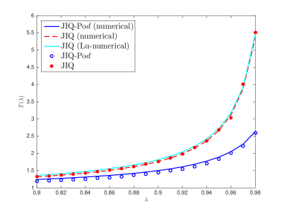
Figure 5 shows the task response times of JIQ and JIQ-Po$d$ obtained from prediction and simulation. As we can see, when the server size is $1000$, the maximum relative error is only $3.4\%$ and the corresponding absolute error is $0.178$. Hence, our theoretical predictions are fairly accurate even for systems of relatively small size. In Figure 5, we also compared the prediction of task response times from [6] with ours. The higher arrival rate is, the more accuracy [6] acquires.

IV-B Impact of “Delete Request” Messages

Recall that in Section II, we applied a “delete request” strategy to the conventional JIQ algorithm (e.g., JIQ-Original) to simplify theoretical analysis. In the subsection, we explore the impact of such “delete request” strategy on our JIQ algorithm in terms of the communication overhead and mean task response time.

Figure 6: Average number of “request” messages per unit time per server of JIQ and JIQ-Original when $r=10$ and $\lambda$ changes from $0.9$ to $0.99$.

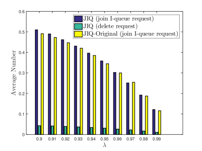
First, idle servers not only send “join I-queue request”, but also send “delete request” under our JIQ algorithm, which will increase the number of “request” messages for each server. Figure 6 studies the average number of “request” messages per unit time per server under JIQ-Original and JIQ. It turns out that the “delete request” only contributes to a small portion of the overall requests. For instance, when $\lambda=0.9$, the number of “delete request” messages is no more than $8\%$ of overall requests.

Second, such “delete request” strategy has little impact on the mean task response time. Figure 8 compares the mean task response times of different JIQ algorithms. It shows that the mean task response times of both JIQ-Original and JIQ are close to each other. To sum up, the “delete request” strategy has little impact on JIQ.

IV-C Comparison of JIQ Algorithms

Finally, we compare our JIQ-Po$d$ with two other variants, JIQ-Threshold and JIQ-SQ($d$) [7, 6].

• JIQ-Threshold: There is a threshold $z$ for server queue length. As long as a server has less than or equal to $z$ tasks, it will send a “join I-queue request” message to an I-queue. Thus, I-queues contain all servers with less than or equal to $z$ tasks.

• JIQ-SQ($d$): When an idle server needs to send a “join I-queue request” message to an I-queue, it adopts the Po$d$ algorithm to select which I-queue to report.

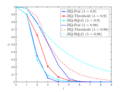
For comparison, we use the tail distribution $\hat{s}_{i}$ and the mean task response time. Figure 7 compares the tail distributions $\hat{s}_{i}$ among those three algorithms when $d=2$ and $z=1$. In Figure 7, the JIQ-Po$d$ algorithm always has the lightest tail in the heavy workload region. Figure 8 compares the mean task response time of different JIQ algorithms. It is shown that the mean task response time of JIQ-Po$d$ is the shortest among five alternative algorithms. Overall, our JIQ-Po$d$ algorithm achieves the best delay performance compared with other alternative JIQ algorithms.

Figure 7: Tail distribution of three algorithms under light workload ($\lambda=0.9$) and heavy workload ($\lambda=0.98$).

Figure 8: A comparison of average task response time for five algorithms.

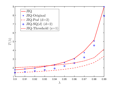
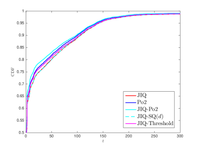
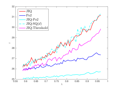
Finally, we conduct trace-driven simulations using real-world data from Google clusters, which contains more than 12,000 tasks over seven hours. In Figure 9, we compare the cumulative distribution function of task response time among five different algorithms. It shows that the JIQ-Po$2$ algorithm attains the best performance when $\lambda=0.88$, $d=2$, $r=10$ (where the threshold is $1$). In Figure 10, we vary the arrival rate $\lambda$ from $0.58$ to $0.96$. We observe that the JIQ-Po$2$ algorithm achieve the shortest mean task response time and the smallest growth rate.

Figure 9: The cumulative distribution function of task response time when $\lambda=0.88$, $d=2$, $r=10$ and threshold is $1$.

Figure 10: A comparison of average task response time for five algorithms.

V Conclusions

In this paper, we analyzed the JIQ algorithm by the mean-field analysis. Then, we proposed a hybrid algorithm called JIQ-Po$d$, which takes the advantage of both JIQ and Po$d$. Under the large-system limit, we obtained semi-closed form expressions of the stationary distributions of JIQ and JIQ-Po$d$. Our theoretical results fit the simulation results well in reasonable large systems, e.g., $N=1000$. In addition, our simulation results show that our JIQ-Po$d$ outperforms many JIQ variants in all conditions.

-A Proof of Theorem 1

Set the potential equation ${V}({\mathbf{z}})$ as

$${V}({\mathbf{z}})=\sum\limits_{i=1}^{N}{z_{i,1}^{2}}+\sum\limits_{i=1}^{N}{z_{i,2}^{2}}$$ (7)

where ${\mathbf{z}}=\left\{{\left({z_{i,1}^{(N)}(t),z_{i,2}^{(N)}(t)}\right)}\right\}_{i=1}^{N}$.

Let ${{q_{{\mathbf{z}},{\mathbf{w}}}}}$ be the transition rate from system state $\mathbf{z}$ to $\mathbf{w}$. The system state changes only when there is a task-arrival or a task-departure event happens. We consider the Lyapunov drift as follows:

$$\begin{split}&\sum\limits_{{\mathbf{w}}\neq{\mathbf{z}}}{{q_{{\mathbf{z}},{\mathbf{w}}}}\left[{{V}({\mathbf{w}})-{V}({\mathbf{z}})}\right]}\\ &=\sum\limits_{{\mathbf{w}}\neq{\mathbf{z}}}{{q_{{\mathbf{z}},{\mathbf{w}}}}\left[{\sum\limits_{i=1}^{N}{(w_{i,1}^{2}-z_{i,1}^{2})}+\sum\limits_{i=1}^{N}{(w_{i,2}^{2}-z_{i,2}^{2})}}\right].}\end{split}$$ (8)

By the Foster-Lyapunov theorem, we only need to show that for any fixed $N$ and $M$,

$$\begin{split}&\sum\limits_{{\mathbf{w}}\neq{\mathbf{z}}}{{q_{{\mathbf{z}},{\mathbf{w}}}}\left[{{V}({\mathbf{w}})-{V}({\mathbf{z}})}\right]}\\ &\leq 2(\lambda-1)\sum\limits_{i=1}^{N}{{z_{i,1}}}+(1+{M^{2}}+\lambda)N\end{split}$$ (9)

This is because:

1. If $\sum\limits_{i=1}^{N}{{z_{i,1}}}>\frac{{(1+{M^{2}}+\lambda)N}}{{2(1-\lambda)}}$, we have

   $$\begin{split}&\sum\limits_{{\mathbf{w}}\neq{\mathbf{z}}}{{q_{{\mathbf{z}},{\mathbf{w}}}}\left[{{V}({\mathbf{w}})-{V}({\mathbf{z}})}\right]}<0.\hfill\\ \end{split}$$

2. If $\sum\limits_{i=1}^{N}{{z_{i,1}}}\leq\frac{{(1+{M^{2}}+\lambda)N}}{{2(1-\lambda)}}$, we have

   $$\begin{split}&\sum\limits_{{\mathbf{w}}\neq{\mathbf{z}}}{{q_{{\mathbf{z}},{\mathbf{w}}}}\left[{{V}({\mathbf{w}})-{V}({\mathbf{z}})}\right]}<\infty.\hfill\\ \end{split}$$

In terms of ${z_{i,2}}$, it increases from $0$ to a positive number in $[1,M]$ when the $i$th server becomes idle. In other cases, ${z_{i,2}}$ remains unchanged or decreases to $0$. As ${z_{i,2}}\in[0,M]$ and the processing rate for each server is $1$, we obtain

$$\sum\limits_{{\mathbf{w}}\neq{\mathbf{z}}}{{q_{{\mathbf{z}},{\mathbf{w}}}}\left[{\sum\limits_{i=1}^{N}{(w_{i,2}^{2}-z_{i,2}^{2})}}\right]}\leq N({M^{2}}-{0^{2}})=N{M^{2}}.$$ (10)

In terms of ${z_{i,1}}$, it increases by $1$ when a task arrives to the $i$th server; it decrease by $1$ when a task departures the $i$th server. Let ${p_{0}^{(N)}}$ be the fraction of empty I-queues. Recall the evolution of a JIQ system, when a new task arrives, we obtain

$$\Pr\{\mbox{meet a non-empty I-queue}\}=1-{p_{0}^{(N)}}$$

and

$$\Pr\{\mbox{meet an empty I-queue}\}={p_{0}^{(N)}}.$$

For task-arrival events, we have

$$\begin{array}[]{l}\sum\limits_{{\mathbf{w}}\neq{\mathbf{z}}}{q_{{\mathbf{z}},{\mathbf{w}}}^{\mbox{(arrival)}}\left[{\sum\limits_{i=1}^{N}{(w_{i,1}^{2}-z_{i,1}^{2})}}\right]}\\ \leq\lambda Np_{0}^{(N)}\sum\limits_{i=1}^{N}{\frac{{{{({z_{i,1}}-1)}^{2}}-z_{i,1}^{2}}}{N}}+\lambda N(1-p_{0}^{(N)})({1^{2}}-{0^{2}})\\ \leq 2\lambda\sum\limits_{i=1}^{N}{{z_{i,1}}}+\lambda N.\end{array}$$

For task-departure events, recall that the server processing rate is $1$, we have

$$\begin{array}[]{l}\sum\limits_{{\mathbf{w}}\neq{\mathbf{z}}}{q_{{\mathbf{z}},{\mathbf{w}}}^{\mbox{(departure)}}\left[{\sum\limits_{i=1}^{N}{(w_{i,1}^{2}-z_{i,1}^{2})}}\right]}\\ \leq\sum\limits_{i=1}^{N}{\left[{{{({z_{i,1}}+1)}^{2}}-z_{i,1}^{2}}\right]}\\ =-2\sum\limits_{i=1}^{N}{{z_{i,1}}}+N.\end{array}$$

Thus, we have

$$\sum\limits_{{\mathbf{w}}\neq{\mathbf{z}}}{{q_{{\mathbf{z}},{\mathbf{w}}}}\left[{\sum\limits_{i=1}^{N}{(w_{i,1}^{2}-z_{i,1}^{2})}}\right]}\leq 2(\lambda-1)\sum\limits_{i=1}^{N}{{z_{i,1}}}+(1+\lambda)N.$$ (11)

Finally, we sum up  (10) and  (11) to have  (9). This completes the proof.

-B $f(p_{0})$ is differentiable and monotonically increasing

First of all, we will show that $f(p_{0})$ is differentiable over the interval $(0,1)$. According to (4), it suffices to prove that

$$h(p_{0})\triangleq{\Gamma\left(\frac{{r+{p_{0}}}}{{{p_{0}}}}\right)-\Gamma\left(\frac{{r+{p_{0}}}}{{{p_{0}}}},r\left(-\lambda+\frac{1}{{{p_{0}}}}\right)\right)}$$

is differentiable over $(0,1)$. Recall that $h(p_{0})$ can be rewritten as

$$h(p_{0})=\int_{0}^{a(p_{0})}g(p_{0},t)dt$$

where $a(p_{0})=r\left(-\lambda+\frac{1}{p_{0}}\right)$ and $g(p_{0},t)=t^{\frac{r}{p_{0}}}e^{-t}$. By the Leibniz’s integral rule, $h(p_{0})$ is differentiable as long as

• $a(p_{0})$ has continuous derivative over $(0,1)$;

• $g(p_{0},t)$ and its partial derivative $\frac{\partial}{\partial p_{0}}g(p_{0},t)$ are continuous in the region of $0<p_{0}<1$ and $0\leq t\leq a(p_{0})$.

Both requirements can be easily verified.

Next, we will show that $f(p_{0})$ is monotonically increasing over $(0,1)$. It suffices to show that $f^{\prime}(p_{0})>0$ over $(0,1)$, since $f(p_{0})$ is differentiable. To this end, we define $g_{i}(p_{0})$ as

$${g_{i}}({p_{0}})\triangleq\left\{\begin{array}[]{l}{p_{0}},i=0,\\ \frac{{{r^{i}}{{(1-\lambda{p_{0}})}^{i}}}}{{\prod\limits_{j=1}^{i}{(r+j{p_{0}})}}}{p_{0}},i\geq 1.\end{array}\right.$$ (12)

Clearly, we have $f(p_{0})=\sum\limits_{i=0}^{\infty}{{g_{i}}({p_{0}})}$. Hence, we need to show that $\sum\limits_{i=0}^{\infty}{{g^{\prime}_{i}}({p_{0}})}>0$. A key observation is the following.

Lemma 1:

If there exists an integer $k$ such that $g^{\prime}_{k}(p_{0})<0$, then for all $i>k$ we have $g^{\prime}_{i}(p_{0})<0$.

Proof:

By  (12), we have

$$g_{i+1}(p_{0})=\frac{{r(1-\lambda{p_{0}})}}{r+(i+1){p_{0}}}g_{i}(p_{0}),\mbox{ for }i\geq 0.$$ (13)

Taking derivatives on both sides, we obtain

$$g^{\prime}_{i+1}(p_{0})=-\frac{{r(r\lambda+(i+1))}}{{{{(r+(i+1){p_{0}})}^{2}}}}g_{i}(p_{0})+\frac{{r(1-\lambda{p_{0}})}}{{r+(i+1){p_{0}}}}g^{\prime}_{i}(p_{0}).$$ (14)

Note that $1-\lambda{p_{0}}>0$. Hence, if $g^{\prime}_{k}(p_{0})<0$, then we have $g^{\prime}_{k+1}(p_{0})<0$. ∎

By Lemma 1, we only need to consider two cases:

1. For all $i\geq 1$, $g^{\prime}_{i}(p_{0})\geq 0$.

2. There exists an integer $k$ such that for all $i<k$, $g^{\prime}_{i}(p_{0})\geq 0$ and for all $i\geq k$, $g^{\prime}_{i}(p_{0})<0$.

For Case 1), we have $\sum\limits_{i=0}^{\infty}{{g^{\prime}_{i}}({p_{0}})}>0$, because $g^{\prime}_{0}(p_{0})=1$ and ${g^{\prime}_{i}}({p_{0}})\geq 0$ when $i\geq 1$.

For Case 2), we need some additional argument. By (13), we have

$$(r+(i+1){p_{0}})g_{i+1}(p_{0})=r(1-\lambda{p_{0}})g_{i}(p_{0}),\mbox{ for }i\geq 0.$$

Hence,

$$\sum_{i=1}^{\infty}(r+i{p_{0}})g_{i}(p_{0})=r(1-\lambda{p_{0}})\sum_{i=0}^{\infty}g_{i}(p_{0}).$$

It follows that

$$\sum\limits_{i=0}^{\infty}{i{g_{i}}(p_{0})}=r-r\lambda\sum\limits_{i=0}^{\infty}{{g_{i}}(p_{0})}$$

and

$$\sum\limits_{i=0}^{\infty}{i{g^{\prime}_{i}}(p_{0})}=-r\lambda\sum\limits_{i=0}^{\infty}{{g^{\prime}_{i}}(p_{0})}.$$

Recall that $k$ is the smallest integer such that $g^{\prime}_{k}(p_{0})<0$. Thus, we have

$$\sum\limits_{i=0}^{\infty}kg^{\prime}_{i}(p_{0})>\sum\limits_{i=0}^{\infty}ig^{\prime}_{i}(p_{0}).$$

Therefore,

$$\sum\limits_{i=0}^{\infty}kg^{\prime}_{i}(p_{0})>-r\lambda\sum\limits_{i=0}^{\infty}{{g^{\prime}_{i}}(p_{0})}.$$

This implies that $\sum\limits_{i=0}^{\infty}{{g^{\prime}_{i}}({p_{0}})}>0$.

References

- [1] E. Schurman and J. Brutlag, “The user and business impact of server delays, additional bytes, and http chunking in web search,” in O’Reilly Velocity Web Performance and Operations Conference, 2009.
- [2] A. Eryilmaz and R. Srikant, “Asymptotically tight steady-state queue length bounds implied by drift conditions,” Queueing Systems: Theory and Applications, vol. 72, no. 3–4, pp. 311–359, Dec. 2012.
- [3] M. Mitzenmacher, “The power of two choices in randomized load balancing,” Ph.D. dissertation, U. C. Berkeley, 1996.
- [4] K. Ousterhout, P. Wendell, M. Zaharia, and I. Stoica, “Sparrow: Distributed, low latency scheduling,” in Proc. of SOSP, Farminton, Pennsylvania, Nov. 3–6, 2013, pp. 69–84.
- [5] L. Ying, R. Srikant, and X. Kang, “The power of slightly more than one sample in randomized load balancing,” in Prof. of INFOCOM, Hong Kong, Apr. 26 – May 1, 2015, pp. 1131–1139.
- [6] Y. Lu, Q. Xie, G. Kliot, A. Geller, J. R. Larus, and A. Greenberg, “Join-idle-queue: A novel load balancing algorithm for dynamically scalable web services,” Performance Evaluation, vol. 68, no. 11, pp. 1056–1071, Nov. 2011.
- [7] M. Mitzenmacher, “Analyzing distributed join-idle-queue: A fluid limit approach,” CoRR, vol. abs/1606.01833, 2016. [Online]. Available: http://arxiv.org/abs/1606.01833
- [8] A. L. Stolyar, “Pull-based load distribution in large-scale heterogeneous service systems,” Queueing Systems, vol. 80, no. 4, pp. 341–361, 2015.
- [9] ——, “Pull-based load distribution among heterogeneous parallel servers: The case of multiple routers,” Queueing Syst. Theory Appl., vol. 85, no. 1-2, pp. 31–65, Feb. 2017.
- [10] S. Foss and A. Stolyar, “Large-scale join-idle-queue system with general service times,” ArXiv e-prints, May 2016.
- [11] C. Wang, C. Feng, and J. Cheng, “Randomized load balancing with a helper,” in Proc. of International Conference on Computing, Networking and Communications (ICNC), Silicon Valley, USA, Jan. 26–29, 2017, pp. 518–524.
- [12] E. Baccarelli, P. Vinueza Naranjo, M. Shojafar, and M. Scarpiniti, “Q*: Energy and delay-efficient dynamic queue management in TCP/IP virtualized data centers,” Computer Communications, vol. 102, pp. 1–37, Dec 2016.
- [13] M. Shojafar, C. Canali, R. Lancellotti, and E. Baccarelli, “Minimizing computing-plus-communication energy consumptions in virtualized networked data centers,” in Proc. of IEEE Symposium on Computers and Communication (ISCC), Messina, Italy, Jan. 27–30, 2016, pp. 1137–1144.
- [14] D. Mukherjee, S. Dhara, S. C. Borst, and J. S. van Leeuwaarden, “Optimal service elasticity in large-scale distributed systems,” ACM Meas. Anal. Comput. Syst., vol. 1, no. 25, pp. 1–28, Jun. 2017.