An Extended Analytic Model for the Heating of Bondwires

Abstract

We present an extended analytic formula for the calculation of the temperature profile along a bondwire embedded in a package. The resulting closed formula is built by coupling the heat transfer equations of the bondwire and the surrounding moulding compound by means of auxiliary variables that stem from an ad-hoc linearisation and mediate the wire-mould thermal interaction. The model, which corrects typical simplifications in previously introduced analytic models, is also optimised against carefully taken experimental samples representing fusing events of bondwires within real packages.

I Introduction

The ever tightening specifications imposed on modern integrated circuits (ICs) by the fast pacing semiconductor industry demand the manufacturing of more energy-efficient chips which are constantly smaller in size. These smart-power ICs must undergo and withstand a whole range of electrostatic discharges (ESD), automotive pulses drive and short-circuit tests which require high currents during short times flowing through the electric connections. Therefore, a good understanding of the interplay of the parameters defining the time-to-failure in these tests is essential to realise cost-effective, robust and fault-tolerant designs.

Among the techniques to establish electric connection between a chip and the lead frame (pins) during device assembly, wire-bonding stands up as the most cost-effective one [1, 2, 3, 4, 5]. In wire-bonding, tiny and fine gold, aluminium, or copper wires are used as electric path between the chip and its package. As miniaturisation of the chips becomes inevitable, the required diameter of the bondwires must also decrease. Since the electric power to the chip must be supplied through these wires, high current densities may occur that heat up the wires causing a substantial increase of their temperature. If the temperature exceeds a predefined value, damage of the compound or bondwire melting are among the most common source of failure in IC devices [3].

From the afore-described scenario, the need among package engineers for an accurate formula that enables the fast dimensioning of bondwires and predicts their safe operation range in a particular application is very important. Ideally, these calculations should be carried out expediently and must involve all the parameters describing a package. Heretofore, several simplified analytic formulas for the calculation of the heating of bondwires and thus the estimation of their current capacities have already been published [1, 2, 3, 4, 5]. However, most of these formulas do not take into account the temperature dependency of the wire parameters and introduced simplifications upon the relevant heat transfer problem that the resulting solution lacks all the geometric information defining the package. In particular, in [1] by retaining the cylindrical symmetry of the wire, the surrounding compound is also deformed into a cylinder in order to facilitate coping with the heat boundary conditions along the wire-compound interface and this is done despite disregarding heat flow along the cross section of the wire. At end, the model only accounts for radially outward heat conduction through a cylindrical moulding compound of infinite extent and provides a loose treatment of the temperature dependency of the wire parameters. More recently in [6], the ideas presented in [1] are expanded. In particular, the moulding compound is still deformed into a material of cylindrical shape upon which on its outer surface either adiabatic or isothermal boundary conditions are imposed. In this manner, a finite cylindrical compound surrounding the wire is considered. The model employs a coupling between the wire and compound heat equations and solves them numerically providing thus the flexibility of analysing current pulses of arbitrary shape. As before, only radial outward heat conduction is accounted for. and the geometric information of the package is again lost.

In this paper, we address these typical shortcomings by developing yet an analytic formulation for the determination of the temperature in bondwires. The more robust analytic formula does involve the essential physical parameters that define the package, i.e., moulding compound material and dimensions, bond-wire characteristics, etc., by using an appropriate set of heat transfer boundary conditions (BCs) and constructing the heat kernel of the compound section. The model couples the wire and compound heat equations and mediates the interaction between them. Subsequent validation of the model is performed and optimisation with experimental data is also carried out.

This paper is organised as follows: In Section II, we formulate the heat transfer problem at hand together with the relevant BCs. In Section III, we provide the solutions to the stated thermal system and perform several numerical tests to validate them. In Section IV, we describe the procedure for optimising the model against experimental data, and also how this data is acquired. This section ends with a comparison on the perfomance of the model before and after optimisation. Finally, in Section V, conclusions are given.

II Problem Formulation

A simple diagram of a classic IC lead-frame package is depicted in Fig. 1.

Figure 1: Diagram of a classic IC lead-frame package.

Because of the often complicate arrangement of the conductors within the package, simplifications are needed to formulate the relevant analytic heat transfer problem.

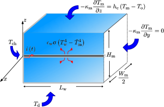
Figure 2: Alternative bondwire heat transfer problem.

In Fig. 2 we depict a simplified parametrical bondwire heat transfer problem. This problem consists of the rectangular compound of height $H_{\text{m}}$ and width $W_{\text{m}}$ that defines the package. The compound is characterised by a homogeneous and isotropic thermal conductivity $\kappa_{\text{m}}$, specific heat $c_{\text{e};\text{m}}$, and mass density $\rho_{\text{m}}$ whose temperature dependence is neglected for simplicity. Similarly, the bondwire of length $L_{\text{w}}$ is characterised by a homogeneous and isotropic thermal conductivity $\kappa_{\text{w}}$, specific heat $c_{\text{e};\text{w}}$, mass density $\rho_{\text{w}}$, and electric resistivity $\uprho_{\text{e};\text{w}}$. The temperature dependence of $\kappa_{\text{w}}$ and $\uprho_{\text{e};\text{w}}$ is taken into account in the calculation of the temperature $T_{\text{w}}(x,y,z,t)$ along the wire, viz.

$$\kappa_{\text{w}}(\widetilde{T}_{\text{w}}) :=\kappa_{\text{o}}\left(1+\alpha_{\kappa}\widetilde{T}_{\text{w}}\right), \quad\uprho_{\text{e;w}}(\widetilde{T}_{\text{w}}) :=\uprho_{\text{e;0}}\left(1+\alpha_{\uprho}\widetilde{T}_{\text{w}}\right),$$ (1)

with $\widetilde{T}_{\text{w}}\equiv T_{\text{w}}-T_{\text{0}}$, $T_{\text{0}}$ the reference (ambient) temperature, $\alpha_{\kappa}$ the temperature coefficient of the thermal conductivity, and $\alpha_{\uprho}$ the temperature coefficient of the electric resistivity. The bondwire will be heated up, during a time $t_{\text{p}}$, by the action of an electric current $i(t)$. We aim at determining the time evolution of $T_{\text{w}}$.

To provide an analytic solution, we impose suitable boundary conditions (BCs) on the domain of interest $\Upomega=[0,W_{\text{m}}]\times[0,L_{\text{w}}]\times[0,H_{\text{m}}]$. Namely, on the rightmost wall, we require that the heat flux mainly occurs through the wire itself (see Fig. 2); therefore, an adiabatic condition is enforced upon this wall, while the wire still remains at the lead temperature $T_{\text{ld}}$, viz.

$$-\kappa_{\text{m}}\frac{\partial}{\partial y}T_{\text{m}}\left(x,L_{\text{w}},z,t\right) =0, \quad T_{\text{w}}\left(x,L_{\text{w}},z,t\right) =T_{\text{ld}}.$$ (2)

Here, $T_{\text{m}}$ is the compound temperature. On the leftmost wall the IC or chip is adjacently located (see Fig. 1); thus we assume a constant temperature $T_{\text{ch}}$ because of the chip high thermal capacitance, viz.

$$T_{\text{m}}\left(x,0,z,t\right) =T_{\text{ch}}, \quad T_{\text{w}}\left(x,0,z,t\right) =T_{\text{ch}}.$$ (3)

On the lateral and top walls of the compound, we assume convective heat transfer because of the background medium [7], viz.

$$-\kappa_{\text{m}}\frac{\partial}{\partial z}T_{\text{m}}\left(x,y,\frac{H_{\text{m}}}{2},t\right) =h_{\text{c}}\left(T_{\text{m}}(x,y,\frac{H_{\text{m}}}{2},t)-T_{0})\right),$$

$$-\kappa_{\text{m}}\frac{\partial}{\partial x}T_{\text{m}}\left(\pm\frac{W_{\text{m}}}{2},y,z,t\right) =h_{\text{c}}\left(T_{\text{m}}(\pm\frac{W_{\text{m}}}{2},y,z,t)-T_{0})\right),$$ (4)

where $h_{\text{c}}$ is the convective transfer coefficient [7]. On the bottom wall, we assume a constant temperature $T_{\text{d}}$ imposed by the die-attach (see Fig. 2), viz.

$$T_{\text{m}}\left(x,y,-\frac{H_{\text{m}}}{2},t\right)=T_{\text{d}}.$$ (5)

Finally on the wire surface $S_{\text{w}}$ we assume that both thermal conductivity and thermal radiation take place. The latter is given by the Stefan-Boltzmann law [7]. Therefore upon the wire-mould interface we state

$$-\int\limits_{S_{\text{w}}}\kappa_{\text{w}}\nabla_{\text{T}}T_{\text{w}}\cdot\mathrm{d}\boldsymbol{S}=\text{TH}_{\text{c}}+\int\limits_{S_{\text{w}}}\epsilon_{\text{w}}\upsigma\left(T^{4}_{\text{w}}-T^{4}_{0}\right)\mathrm{d}S,$$ (6)

where $\nabla_{\text{T}}T_{\text{w}}$ is the transverse gradient of the wire temperature, that is the gradient along the $xz$-plane (see Fig. 2), TH${}_{\text{c}}$ just denotes the conductive part of the thermal flux that occurs on the wire surface, $\epsilon_{\text{w}}$ is the wire emissivity [7], and $\upsigma$ is the Stefan-Boltzmann constant [7].

II-A Bondwire Heat Equation

The heat equation for a stationary wire of constant mass density reads [7]

$$\rho_{\text{w}}c_{\text{e;w}}\frac{\partial T_{\text{w}}}{\partial t}=\nabla\cdot\left(\kappa_{\text{w}}\nabla T_{\text{w}}\right)+\dot{q}_{\text{i}},$$ (7)

where $\dot{q}_{\text{i}}$ is the impressed volumetric thermal power density within the wire. By expanding the above gradient operator as $\nabla=\partial_{y}\boldsymbol{a}_{y}+\nabla_{\text{T}}$, with $\boldsymbol{a}_{y}$ the unit vector along the $y$-axis, and assuming that the Biot number [7] of the wire is small along the $xz$-plane , that is $T_{\text{w}}$ mainly varies along the wire axis, we may express (7) by means of (6) in a form that explicitly involves the radiation condition, viz.

$$\rho_{\text{w}}c_{\text{e};\text{w}}\frac{\partial}{\partial t}T_{\text{w}}=\frac{\partial}{\partial y}\left(\kappa_{\text{w}}\frac{\partial}{\partial y}T_{\text{w}}\right)-\epsilon_{\text{w}}\upsigma\left(T^{4}_{\text{w}}-T^{4}_{0}\right)\frac{C_{\text{w}}}{A_{\text{w}}}+\dot{q}_{\text{i}},$$ (8)

where $A_{\text{w}}(y)$ and $C_{\text{w}}(y)$ are the cross-section area and perimeter of the wire, respectively. In (8) we may think as if the contribution of TH${}_{\text{c}}$ is apparently vanished. However, as we will see in section III, the contribution of TH${}_{\text{c}}$ is again accounted for with the introduction of a linearising constant in the wire and compound heat equations.

II-B Moulding Compound Heat Equation

The moulding compound heat equation in integral form reads [7, 8]

$$\rho_{\text{m}}c_{\text{e;m}}\frac{\partial}{\partial t}\int\limits_{V_{\text{m}}}T_{\text{m}}\mathrm{d}V=\kappa_{\text{m}}\int\limits_{S_{\text{w}}}\nabla T_{\text{m}}\cdot\mathrm{d}\boldsymbol{S}+\kappa_{\text{m}}\int\limits_{\tilde{S}_{\text{m}}}\nabla T_{\text{m}}\cdot\mathrm{d}\boldsymbol{S},$$ (9)

where $V_{\text{m}}$ is the compound volume, $S_{\text{w}}$ is the wire-compound common interface, and $\tilde{S}_{\text{m}}$ is the compound remaining surface. With the help of (6) and the low-Biot-number assumption, we may express (9) as follows

$$\rho_{\text{m}}c_{\text{e;m}}\frac{\partial}{\partial t}\int\limits_{V_{\text{m}}}T_{\text{m}}\mathrm{d}V=\kappa_{\text{m}}\int\limits_{\tilde{S}_{\text{m}}}\nabla T_{\text{m}}\cdot\mathrm{d}\boldsymbol{S}+\\ \int\limits_{V_{\text{w}}}\epsilon_{\text{w}}\upsigma\left(T^{4}_{\text{w}}-T^{4}_{0}\right)\frac{C_{\text{w}}}{A_{\text{w}}}\mathrm{d}V,$$ (10)

with $V_{\text{w}}$ the wire volume. The above equation permits to regard the problem at hand by one in which the wire is considered infinitesimally thin. To this end, we take $\lim_{A_{\text{w}}\rightarrow 0}$ on (10); thus, this can be written point-wise as follows

$$\rho_{\text{m}}c_{\text{e;m}}\frac{\partial}{\partial t}T_{\text{m}}=\kappa_{\text{m}}\nabla^{2}T_{\text{m}}+\epsilon_{\text{w}}\upsigma\left(T^{4}_{\text{w}}-T^{4}_{0}\right)C_{\text{w}}\delta(x)\delta(z),$$ (11)

where $\delta(.)$ is the Dirac delta [9]. Equation (11) is the heat equation of the compound with the wire as an impressed heat source, and its solution involves the heat kernel (Green’s function) of the compound [10].

III Heat Transfer Problem Solution

Equations (8) and (11) constitute a non-linear coupled thermal system. In this section, we carry out the solution of this system by means of an ad-hoc linearisation.

III-A Bondwire Solution

We start by linearising the radiation term in (8) as follows

$$\begin{split}T^{4}_{\text{w}}-T^{4}_{0}&=\left(T^{3}_{\text{w}}+T^{2}_{\text{w}}T_{0}+T_{\text{w}}T^{2}_{0}+T^{3}_{0}\right)\left(T_{\text{w}}-T_{0}\right)\\ &\approx\chi_{\text{w}}\left(T_{\text{w}}-T_{0}\right),\end{split}$$ (12)

with $\chi_{\text{w}}$ a constant. This approximation is reasonable insofar as thermal radiation is not the heat transfer dominant term [7]. Therefore in this manner, with the introduction of the constant $\chi_{\text{w}}$ we are globing in one both the contribution of conduction and radiation to the thermal flux at the wire surface. Next, we employ the following transformation

$$\widetilde{\theta}_{\text{w}}\left(\widetilde{T}_{\text{w}}\right):=\frac{1}{\kappa_{0}}\int\limits_{0}^{\widetilde{T}_{\text{w}}}\kappa_{\text{w}}\left(s\right)\mathrm{d}s,$$ (13)

which implies that $\widetilde{\theta}_{\text{w}}=\widetilde{T}_{\text{w}}+\alpha_{\kappa}/2\,\widetilde{T}^{2}_{\text{w}}$ and $\partial_{y}\widetilde{\theta}_{\text{w}}=\kappa_{\text{w}}/\kappa_{0}\,\partial_{y}\widetilde{T}_{\text{w}}$; thus, enabling us to write (8) as

$$\rho_{\text{w}}c_{\text{e};\text{w}}\frac{\partial}{\partial t}\widetilde{\theta}_{\text{w}}=\kappa_{\text{o}}\frac{\partial^{2}}{\partial y^{2}}\widetilde{\theta}_{\text{w}}-F_{\text{o;w;r}}\widetilde{\theta}_{\text{w}}+G_{\text{o;w}}+\frac{1}{2}H_{\text{o;w;r}},$$ (14)

with

$$G_{\text{o;w}} =\frac{I^{2}_{0}\uprho_{\text{e;o}}}{A^{2}_{\text{w}}}, \quad F_{\text{o;w;r}} =\epsilon_{\text{w}}\upsigma\chi_{\text{w}}\frac{C_{\text{w}}}{A_{\text{w}}},$$

$$H_{\text{o;w;r}}=\frac{2I^{2}_{0}\uprho_{\text{e;o}}\alpha_{\uprho}\widetilde{T}_{\text{w;e}}}{A^{2}_{\text{w}}}+\epsilon_{\text{w}}\upsigma\chi_{\text{w}}\frac{C_{\text{w}}}{A_{\text{w}}}\alpha_{\kappa}\widetilde{T}^{2}_{\text{w;e}},$$ (15)

and where we have approximated $\partial_{t}\widetilde{\theta}_{\text{w}}\approx\partial_{t}\widetilde{T}_{\text{w}}$ so as to keep linear the transient term in (14) and have introduced $\widetilde{T}_{\text{w;e}}$ as an auxiliary constant dubbed the wire effective temperature.

We solve (14) by separation of variables with $\widetilde{\theta}_{\text{w}}(y,t)=\tilde{\theta}_{\text{w};1}(y,t)+\tilde{\theta}_{\text{w};2}(y)$, thus yielding

$$\begin{split}\tilde{\theta}_{\text{w}}(y,t)&=\sum_{k}C^{\text{t}}_{\text{w};k;\text{r}}e^{-\frac{\kappa_{\text{o}}}{\rho_{\text{w}}c_{\text{e;w}}}\lambda^{2}_{y;\text{w},k}t}e^{-\frac{F_{\text{o;w;r}}}{\rho_{\text{w}}c_{\text{e;w}}}t}\sin\left(\lambda_{y;\text{w},k}y\right)\\ &+C^{\text{s}}_{1;y;\text{w;r}}\cosh\left(\sqrt{\frac{F_{\text{o;w;r}}}{\kappa_{\text{o}}}}y\right)+C^{\text{s}}_{2;y;\text{w;r}}\sinh\left(\sqrt{\frac{F_{\text{o;w;r}}}{\kappa_{\text{o}}}}y\right)\\ &+\frac{1}{2}\frac{H_{\text{o;w;r}}}{F_{\text{o;w;r}}}+\frac{G_{\text{o;w}}}{F_{\text{o;w;r}}};\;\lambda_{y;\text{w},k}=\frac{k\pi}{L_{\text{w}}},\,k>0.\end{split}$$ (16)

Above, the coefficients $\{C^{\text{t}}_{\text{w};k;\text{r}},C^{\text{s}}_{1;y;\text{w;r}},C^{\text{s}}_{2;y;\text{w;r}}\}$ are determined by means of the initial condition at $t=0$ and the relevant BCs in (2) and (3), respectively. We observe that the auxiliary constants $\widetilde{T}_{\text{w;e}}$ and $\chi_{\text{w}}$ in (15) are yet to be determined.

III-B Moulding Compound Solution

Let us rewrite (11) with the help of $\chi_{\text{w}}$, viz.

$$\rho_{\text{m}}c_{\text{e;m}}\frac{\partial}{\partial t}T_{\text{m}}=\kappa_{\text{m}}\nabla^{2}T_{\text{m}}+\epsilon_{\text{w}}\upsigma\chi_{\text{w}}\widetilde{T}_{\text{w}}C_{\text{w}}\delta(x)\delta(z).$$ (17)

We notice in (17) that if the impressed source were zero, the compound temperature would be solely imposed by the chip and die-attach temperatures (see Fig. 2). Once the electric current is switched on, another temperature component superimpose. Let us denote by $T_{\text{m}}$ the first of these components and solve for it by defining $\widetilde{T}_{\text{m}}\equiv T_{\text{m}}-T_{0}$, expanding $\widetilde{T}_{\text{m}}\left(x,y,z,t\right)=\widetilde{T}_{\text{m};1}\left(x,y,z,t\right)+\widetilde{T}_{\text{m};2;1}\left(x,y,z\right)+\widetilde{T}_{\text{m};2;2}\left(x,y,z\right)$, and substituting in (17) together with BCs (2)–(5). The second component is obtained by means of the compound heat kernel (Green’s function). In Appendix A, we briefly describe how these component functions are exactly determined.

Having calculated the aforementioned temperature components, the moulding compound temperature can be expressed as

$$T_{\text{m}}\left(x,y,z,t\right)=T_{0}+\widetilde{T}_{\text{m};1}\left(x,y,z,t\right)+\widetilde{T}_{\text{m};2;1}\left(x,y,z\right)+\\ \widetilde{T}_{\text{m};2;2}\left(x,y,z\right)+\int\limits_{0}^{t}\int\limits_{0}^{L_{\text{w}}}G_{\text{m}}\left(x,y,z,t-\tau,y^{\prime}\right)\dot{q}_{\text{i}}\left(y^{\prime},\tau\right)\mathrm{d}y^{\prime}\mathrm{d}\tau,$$

$$\dot{q}_{\text{i}}\left(y^{\prime},\tau\right)=\epsilon_{\text{w}}\upsigma\chi_{\text{w}}\widetilde{T}_{\text{w}}\left(y^{\prime},\tau\right)C_{\text{w}}.$$ (18)

The above expression provides the temperature at any point within the compound for any time-variant current. Both auxiliary constants $\widetilde{T}_{\text{w;e}}$ and $\chi_{\text{w}}$ also appear in (18) within $\widetilde{T}_{\text{w}}\left(y^{\prime},\tau\right)$. In Appendix B, we describe how these two constants are determined by mediating the thermal interaction between the compound and the wire.

III-C Numerical Test

We have implemented the afore-described model and have performed numerical tests for Gold ($\mathrm{Au}$), Copper ($\mathrm{Cu}$), and Aluminium ($\mathrm{Al}$) wires of diameters $D_{\text{w}}=\{0.8,1.0,\ldots,1.8,2.0\}\,\mathrm{mil}$ and length $L_{\text{w}}=2.5\,\mathrm{mm}$. A moulding compound with $W_{\text{m}}=4.45\,\mathrm{mm}$ and $H_{\text{m}}=1.48\,\mathrm{mm}$, and made of an Epoxy resin with $\kappa_{\text{m}}=0.870\,\mathrm{W/(m\cdot K)}$, $c_{\text{e};\text{m}}=882\,\mathrm{J/(Kg\cdot K)}$, and $\rho_{\text{m}}=1860\,\mathrm{kg/m^{3}}$ is assumed.

To verify our solution, we compute $T_{\text{m}}$ at the $xy$- and $yz$-planes (see Fig. 2) for an $\mathrm{Au}$-wire of $D_{\text{w}}=2\,\mathrm{mil}$, which carries an electric current of $I_{0}=3.7\,\mathrm{A}$ during a time $t_{\text{p}}=500\,\mathrm{ms}$. In concrete, we want verify the compound temperature expansion coefficients (see Appendix A) when satisfying the relevant BCs. We have also assumed herein that $T_{\text{ch}}=80\,\mathrm{{}^{\circ}C}$, $T_{\text{ld}}=40\,\mathrm{{}^{\circ}C}$, $T_{\text{d}}=35\,\mathrm{{}^{\circ}C}$, $T_{0}=20\,\mathrm{{}^{\circ}C}$, and $h_{\text{c}}=25\,\mathrm{W/(m^{2}\cdot K)}$.

(a)

(b)

(c)

(d)

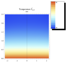
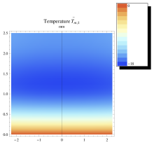
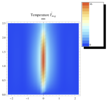
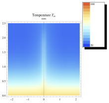
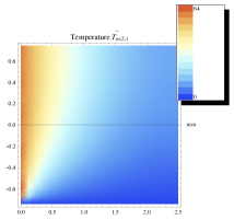
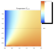
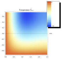
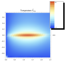
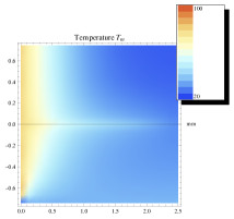
Figure 3: Compound temperature components at the $xy$-plane (top view) and $t=500\,\mathrm{ms}$; (a) steady $\widetilde{T}_{\text{m};2}=\widetilde{T}_{\text{m};2,1}+\widetilde{T}_{\text{m};2,2}$ component; (b) transient $\widetilde{T}_{\text{m};1}$ component; (c) heat kernel $\widetilde{T}_{\text{m;g}}$ component; (d) compound temperature $T_{\text{m}}$. The $\mathrm{Au}$-wire is depicted as a straight line.

(a)

(b)

(c)

(d)

(e)

Figure 4: Compound temperature components at the $yz$-plane (side view) and $t=500\,\mathrm{ms}$; (a) steady $\widetilde{T}_{\text{m};2,1}$ component; (b) steady $\widetilde{T}_{\text{m};2,2}$ component; (c) transient $\widetilde{T}_{\text{m};1}$ component; (d) heat kernel $\widetilde{T}_{\text{m;g}}$ component, (e) compound temperature $T_{\text{m}}$. The $\mathrm{Au}$-wire is depicted as a straight line.

Fig. 3 and 4 show the plots of the temperature component in (18) depicting the wire as a straight line. For example, Fig. 3a shows a top-view plot of the steady component $\widetilde{T}_{\text{m};2}=\widetilde{T}_{\text{m};2,1}+\widetilde{T}_{\text{m};2,2}$, whereas Fig. 4a and 4b shows a side-view plot of it separated into its constitutives $T_{\text{m};2,1}$ and $T_{\text{m};2,2}$. In particular Fig. 3a, 4a, and 4b show that the steady component $\widetilde{T}_{\text{m};2}$ along the chip and die-attach planes satisfies the required BCs in (34) and (35). Fig. 3b and 4c show the plot of the transient component $T_{\text{m};1}$, and as we can note, this component amounts to $\widetilde{T}_{\text{m};1}=0$ along the chip and die-attach planes, thus verifying the required BCs in (34) and (35).

Fig. 3c and 4d shows the plot of the heat kernel component $\widetilde{T}_{\text{m;g}}$, that is the integral in (18). These plots suggest that heat flux propagates radially away from the wire into the compound and show a maximum that occurs at the wire mid-point while two minima appear towards the extremes of the wire. We also notice that this component is consistent with the required BCs along the chip and die-attach planes, where it vanishes. Finally in Fig. 3d and 4e, the combined action of all these components; namely, the compound temperature $T_{\text{m}}$ is plotted. In particular, we can notice therein that $T_{\text{m}}=T_{\text{ch}}=80\,\mathrm{{}^{\circ}C}$ and $T_{\text{m}}=T_{\text{d}}=35\,\mathrm{{}^{\circ}C}$ along the chip and die-attach planes as demanded by the BCs. Furthermore, most of the compound is slightly above the (ambient) temperature $T_{0}=20\,\mathrm{{}^{\circ}C}$ used as the initial condition due to its low thermal conductivity. Nevertheless, we may expect the compound to become hotter as time progresses. It is important here to remark that $T_{\text{m}}$ is more an auxiliary scalar field that helps to estimate the effect of the compound on the wire temperature, rather than the true compound temperature.

(a) $\mathrm{Al}$-wire

(b) $\mathrm{Au}$-wire

(c) $\mathrm{Cu}$-wire

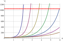
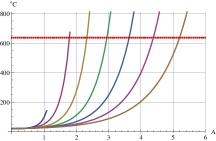
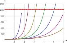
Figure 5: Bondwire current capacities for diameters $D_{\text{w}}=\{0.8,1.0,\ldots,1.8,2.0\}\,\mathrm{mil}$ and $L_{\text{w}}=2.5\,\mathrm{mm}$; a) $\mathrm{Al}$-wire; b) $\mathrm{Au}$-wire; c) $\mathrm{Cu}$-wire. The horizontal dotted line indicates the melting temperature.

Fig. 5 shows the estimated current capacity $T_{\text{w}}$ vs $I_{0}$ after a time of $50\,\mathrm{ms}$ for $\mathrm{Al}$-, $\mathrm{Au}$-, and $\mathrm{Cu}$-wires. The temperature $T_{\text{w}}$ plotted therein is at the wire mid-point. The results in Fig. 5 reveals current capacities lower than those estimated in [1] under similar setting. In other words, for a given bondwire configuration, the current amplitude in [1] that causes the wire to fuse after a certain time is higher than the amplitude estimated by our model. This seems to indicate a tendency of the model in [1] to underestimate the temperature in bondwires. Fig. 5 also demonstrates the capabilities of our model to provide a safe range of operation for the bondwires before melting and moulding deterioration is reached.

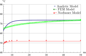
Figure 6: Temperature $T_{\text{w}}$ of the wire mid-point in time for a gold bondwire of length $L_{\text{w}}=2.5\,\mathrm{mm}$ and diameter $D_{\text{w}}=2.0\,\mathrm{mil}$. The current amplitude amounts to $I_{0}=2\,\mathrm{A}$.

Fig. 6 shows the a comparison between our analytic model and an implementation of Noebauer’s model [1]. For the reference, we have also included the solution obtained via a 3-D FEM simulation of the single bondwire heat problem depicted in Fig. 1. Clearly, the model in [1] underestimates the temperature profile. Similar results have been obtained for the other wire materials, namely copper and aluminium. Having verified numerically our solution, in the next section we conduct the optimisation of our model.

IV Bondwire Model Optimisation

As in any analytic model built upon simplifications, optimisation based on experimental data is necessary. In a real package, where bondwires are tightly disposed, the overall temperature distribution is governed by a non-linear thermo-electromagnetic coupling mechanism. Furthermore, the manufacturing imperfections, mould compound degradation, and current-induced ageing of the wires add uncertainties that are certainly not accounted for by a simplified analytic model. Hence, to counteract the accumulated effect of these uncertainties in the accuracy of the model, we carry out parameter optimisation in this section.

IV-A Optimisation Problem Statement

Let us consider the bondwire model as a function $\mathrm{B}_{\text{w}}:\underline{\mathbf{p}}\times\left(I_{0},t_{\text{p}}\right)\longmapsto T_{\text{w}}$ with $\underline{\mathbf{p}}=\left[\mathrm{p}_{1},\mathrm{p}_{2},\ldots,\mathrm{p}_{N_{\text{p}}}\right]^{{}^{\!\top}}$; namely a mapping from a parameter space $\underline{\mathbf{p}}$ into the temperature $T_{\text{w}}$ for a given pair $\left(I_{0},t_{\text{p}}\right)$ of the amplitude and duration of the current. Experimentally, we have collected a set of data $\left\{I_{0,i},t_{\text{p},i}\right\}$, with $i=1,\ldots,N_{\text{d}}$ that represents fusing events, that is the current amplitude $I_{0}$ with duration $t_{\text{p}}$ that causes a bondwire sample to fuse. In this optimisation we assume that fusing occurs at the wire mid-point where the hottest spot is expected [2, 3, 5]. In this manner, we define the model residual $\mathrm{R}_{\text{w},i}$ as follows

$$\mathrm{R}_{\text{w},i}(\underline{\mathbf{p}})\coloneqq\lvert T_{\text{w;f}}-\mathrm{B}_{\text{w}}\left(\underline{\mathbf{p}},I_{0,i},t_{\text{p},i}\right)\rvert^{2},$$ (19)

where $T_{\text{w;f}}$ is the corresponding fusing temperature, and $\mathrm{B}_{\text{w}}\left(\underline{\mathbf{p}},I_{0,i},t_{\text{p},i}\right)$ is the model estimation at the mid-point for a given $\left(I_{0,i},t_{\text{p},i}\right)$. Hence, the total residual for a set of experimental data will be

$$\begin{split}\mathrm{R}_{\text{w}}\left(\underline{\mathbf{p}}\right)&=\sum_{i=1}^{N_{\text{d}}}\mathrm{R}_{\text{w},i}(\underline{\mathbf{p}})\\ &=\left(\underline{\mathbf{T}}_{\text{w}}-\underline{\mathbf{B}}_{\text{w}}\left(\underline{\mathbf{p}}\right)\right)^{{}^{\!\top}}\cdot\left(\underline{\mathbf{T}}_{\text{w}}-\underline{\mathbf{B}}_{\text{w}}\left(\underline{\mathbf{p}}\right)\right)\\ &=\underline{\mathbf{T}}_{\text{w}}^{{}^{\!\top}}\cdot\underline{\mathbf{T}}_{\text{w}}-2\underline{\mathbf{T}}_{\text{w}}^{{}^{\!\top}}\cdot\underline{\mathbf{B}}_{\text{w}}\left(\underline{\mathbf{p}}\right)+\underline{\mathbf{B}}_{\text{w}}\left(\underline{\mathbf{p}}\right)^{{}^{\!\top}}\cdot\underline{\mathbf{B}}_{\text{w}}\left(\underline{\mathbf{p}}\right),\end{split}$$ (20)

with

$$\underline{\mathbf{T}}_{\text{w}} =\begin{bmatrix}T_{\text{w;f}}\\ T_{\text{w;f}}\\ \vdots\\ T_{\text{w;f}}\end{bmatrix}, \quad\underline{\mathbf{B}}_{\text{w}}\left(\underline{\mathbf{p}}\right) =\begin{bmatrix}\mathrm{B}_{\text{w}}\left(\underline{\mathbf{p}},I_{0,1},t_{\text{p},1}\right)\\ \mathrm{B}_{\text{w}}\left(\underline{\mathbf{p}},I_{0,2},t_{\text{p},2}\right)\\ \vdots\\ \mathrm{B}_{\text{w}}\left(\underline{\mathbf{p}},I_{0,N_{\text{d}}},t_{\text{p},N_{\text{d}}}\right)\end{bmatrix}.$$ (21)

Here, we want to determine $\underline{\mathbf{p}}^{\star}$ that minimises (20), viz.

$$\underline{\mathbf{p}}^{\star}\equiv\underset{\underline{\mathbf{p}}}{\operatorname{arg}\,\operatorname{min}}\;\mathrm{R}_{\text{w}}\left(\underline{\mathbf{p}}\right).$$ (22)

IV-B Parameter Sub-Set Identification

We solve for $\underline{\mathbf{p}}^{\star}$ in (22) by using a Newton-Raphson method [11] with an order reduction strategy that splits the space $\underline{\mathbf{p}}$ into well- and ill-conditioned parameters [12, 13, 14]. In this manner, robust optimisation is accomplished.

The Newton-Raphson method for our multidimensional optimisation problem is characterised by the system

$$\underline{\underline{\mathbf{H}}}_{\mathrm{R}_{\text{w}}}\cdot\Delta\underline{\mathbf{p}}=-\underline{\mathbf{J}}_{\mathrm{R}_{\text{w}}}^{{}^{\!\top}},$$ (23)

where $\Delta\underline{\mathbf{p}}=\underline{\mathbf{p}}_{k+1}-\underline{\mathbf{p}}_{k}$ is the difference between the next estimation $\underline{\mathbf{p}}_{k+1}$ and the actual one $\underline{\mathbf{p}}_{k}$, $\underline{\mathbf{J}}_{\mathrm{R}_{\text{w}}}$ and $\underline{\underline{\mathbf{H}}}_{\mathrm{R}_{\text{w}}}$ are the Jacobian and Hessian matrices of the residual [15] evaluated at $\underline{\mathbf{p}}_{k}$. Let us now assume that we have carried out the SVD of $\underline{\underline{\mathbf{H}}}_{\mathrm{R}_{\text{w}}}$ and have ordered the singular values within $\underline{\underline{\mathbf{\Sigma}}}_{\mathrm{R}_{\text{w}}}$ in decreasing order of magnitude. Then we nullify the entries of the smallest singular values in $\underline{\underline{\mathbf{\Sigma}}}_{\mathrm{R}_{\text{w}}}$ so as to approximate

$$\underline{\underline{\mathbf{\Sigma}}}_{\mathrm{R}_{\text{w}}}\approx\underline{\underline{\widetilde{\mathbf{\Sigma}}}}_{\mathrm{R}_{\text{w}}}=\begin{bmatrix}\underline{\underline{\mathbf{\Sigma}}}_{\mathrm{R}_{\text{w}},\text{uu}}&\underline{\underline{\mathbf{0}}}\\ \underline{\underline{\mathbf{0}}}&\underline{\underline{\mathbf{0}}}\end{bmatrix},$$ (24)

that is we cancel out the diagonal sub-matrix $\underline{\underline{\mathbf{\Sigma}}}_{\mathrm{R}_{\text{w}},\text{ll}}$ of smallest singular values, and the order of $\underline{\underline{\widetilde{\mathbf{\Sigma}}}}_{\mathrm{R}_{\text{w}}}$ determines the number of well-conditioned parameters. Approximation (24) leads to

$$\underline{\underline{\mathbf{H}}}_{\mathrm{R}_{\text{w}}}\approx\underline{\underline{\widetilde{\mathbf{H}}}}_{\mathrm{R}_{\text{w}}}=\underline{\underline{\mathbf{V}}}_{\mathrm{R}_{\text{w}},\text{1u}}\cdot\underline{\underline{\mathbf{\Sigma}}}_{\mathrm{R}_{\text{w}},\text{uu}}\cdot\underline{\underline{\mathbf{V}}}_{\mathrm{R}_{\text{w}},\text{u1}}^{\text{H}},$$ (25)

where $\underline{\underline{\mathbf{V}}}_{\mathrm{R}_{\text{w}},\text{1u}}$ is the matrix stemming from $\underline{\underline{\mathbf{V}}}_{\mathrm{R}_{\text{w}}}$ after cancelling out the singular vectors associated with the nullified singular values.

To identify the well-conditioned parameters of (23), we perform the QR-decomposition (with permutation) of $\underline{\underline{\mathbf{V}}}_{\mathrm{R}_{\text{w}},\text{u1}}^{\text{H}}$ [15], viz.

$$\underline{\underline{\mathbf{V}}}_{\mathrm{R}_{\text{w}},\text{u1}}^{\text{H}}\cdot\underline{\underline{\mathbf{P}}} =\underbrace{\begin{bmatrix}\underline{\underline{\mathbf{V}}}_{\mathrm{R}_{\text{w}},\text{uu}}^{\text{H}}&\underline{\underline{\mathbf{V}}}_{\mathrm{R}_{\text{w}},\text{ul}}^{\text{H}}\end{bmatrix}}_{\underline{\underline{Q}}\cdot\underline{\underline{R}}}\Rightarrow \;\underline{\underline{\mathbf{P}}}^{{}^{\!\top}}\cdot\underline{\underline{\mathbf{V}}}_{\mathrm{R}_{\text{w}},\text{1u}} =\underbrace{\begin{bmatrix}\underline{\underline{\mathbf{V}}}_{\mathrm{R}_{\text{w}},\text{uu}}\\ \underline{\underline{\mathbf{V}}}_{\mathrm{R}_{\text{w}},\text{lu}}\end{bmatrix}}_{\underline{\underline{R}}^{{}^{\!\top}}\cdot\underline{\underline{Q}}^{{}^{\!\top}}}.$$ (26)

Above, the permutation matrix $\underline{\underline{\mathbf{P}}}$ swaps columns of $\underline{\underline{\mathbf{V}}}_{\mathrm{R}_{\text{w}},\text{u1}}^{\text{H}}$ to split them into a set of linearly independent singular vectors $\underline{\underline{\mathbf{V}}}_{\mathrm{R}_{\text{w}},\text{uu}}^{\text{H}}$ and a set of linearly dependent singular vectors $\underline{\underline{\mathbf{V}}}_{\mathrm{R}_{\text{w}},\text{ul}}^{\text{H}}$. This splitting permits to separate the set of well-posed parameters from the ill-posed ones. Identities (25) and (26) lead to the sought reduced counterpart of (23), viz.

$$\underline{\underline{\widetilde{\mathbf{H}}}}_{\mathrm{R}_{\text{w}},\text{uu}}\cdot\Delta\underline{\widetilde{\mathbf{p}}}_{\text{u}}=-\underline{\mathbf{J}}_{\mathrm{R}_{\text{w}},\text{u}}^{{}^{\!\top}},$$ (27)

with

$$\underline{\underline{\widetilde{\mathbf{H}}}}_{\mathrm{R}_{\text{w}},\text{uu}} =\underline{\underline{\mathbf{V}}}_{\mathrm{R}_{\text{w}},\text{uu}}\cdot\underline{\underline{\mathbf{\Sigma}}}_{\mathrm{R}_{\text{w}},\text{uu}}\cdot\underline{\underline{\mathbf{V}}}_{\mathrm{R}_{\text{w}},\text{uu}}^{\text{H}}; \quad\underline{\underline{\mathbf{P}}}^{{}^{\!\top}}\cdot\Delta\underline{\mathbf{p}} =\begin{bmatrix}\Delta\underline{\widetilde{\mathbf{p}}}_{\text{u}}\\ \underline{\mathbf{0}}\end{bmatrix};$$

$$\underline{\underline{\mathbf{P}}}^{{}^{\!\top}}\cdot\underline{\mathbf{J}}_{\mathrm{R}_{\text{w}}}^{{}^{\!\top}}=\begin{bmatrix}\underline{\mathbf{J}}_{\mathrm{R}_{\text{w}},\text{u}}^{{}^{\!\top}}\\ \underline{\mathbf{J}}_{\mathrm{R}_{\text{w}},\text{l}}^{{}^{\!\top}}\end{bmatrix},$$ (28)

where we group and retain in (27) the entries corresponding to the well-posed parameters, while setting constant the ill-posed ones by stating that $\Delta\underline{\widetilde{\mathbf{p}}}_{\text{l}}=\underline{\mathbf{0}}$ in (28).

Finaly, we express $\underline{\mathbf{J}}_{\mathrm{R}_{\text{w}}}$ and $\underline{\underline{\mathbf{H}}}_{\mathrm{R}_{\text{w}}}$ in terms of $\underline{\underline{\mathbf{J}}}_{\mathrm{B}_{\text{w}}}$ and $\underline{\underline{\mathbf{H}}}_{\mathrm{B}_{\text{w}}}$; namely, the Jacobian and Hessian matrices of the bondwire model $\mathrm{B}_{\text{w}}$. Further mathematical analysis shows that these matrices are related as follows

$$\underline{\mathbf{J}}_{\mathrm{R}_{\text{w}}} =2\left(\underline{\mathbf{B}}^{{}^{\!\top}}_{\text{w}}\left(\underline{\mathbf{p}}\right)-\underline{\mathbf{T}}^{{}^{\!\top}}_{\text{w}}\right)\cdot\underline{\underline{\mathbf{J}}}_{\mathrm{B}_{\text{w}}},$$ (29)

$$\underline{\underline{\mathbf{H}}}_{\mathrm{R}_{\text{w}}} =2\underline{\underline{\mathbf{J}}}^{{}^{\!\top}}_{\mathrm{B}_{\text{w}}}\cdot\underline{\underline{\mathbf{J}}}_{\mathrm{B}_{\text{w}}}+2\sum_{i=1}^{N_{\text{d}}}\left(\mathrm{B}_{\text{w}}\left(\underline{\mathbf{p}},I_{0,i},t_{\text{p},i}\right)-T_{\text{w;f}}\right)\underline{\underline{\mathbf{H}}}_{\mathrm{B}_{\text{w}},i}.$$ (30)

In the next section, we briefly describe the experimental setup used to generate and measure the required bondwire fusing events.

IV-C Experimental Setup

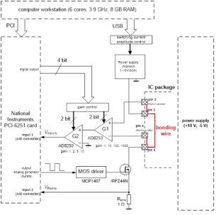
The experimental setup for the extraction of fusing events and the dynamical parameters of the encapsulated bondwires is described in this section. In Fig. 7 we show the schematic of the so-called bondwire tester. The setup permits statistical quantification of the current capabilities and fatigue of the bondwires. All integrated circuits and Kelvin probes were fabricated by ON-Semiconductor (Belgium).

Figure 7: Schematic of the bondwire tester.

The tester consists of a power supply ($16\,\mathrm{V}$ and $60\,\mathrm{A}$), a test interface (custom made board), a personal computer (with MATLAB™), and a data acquisition card (DAQ) (National Instruments 6251) capable of capturing $1\,\mathrm{MS/s}$ multichannel, $16\,\mathrm{bit}$ resolution and with a voltage range of $\pm 10\,\mathrm{V}$. The test interface consists of six power channels (for six bondwire pairs). To avoid using 12 acquisition channels, each channel is addressed by demultiplexing the driving signal to a specific bondwire. Thus, the current flowing through and the voltage drop along the bondwire are sensed, amplified, and multiplexed to outputs which are digitised by a NI card and thus returned back to the computer.

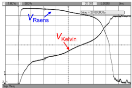
Figure 8: Details of $V_{\text{Rsens}}$ and $V_{\text{Kelvin}}$ captured with the oscilloscope.

In general, the experimental setup can be divided into two parts, namely the software which directly controls the NI card and consequently the tester, and the printed circuit board (PCB) of the tester with the multichannel switching power source. Each bondwire is addressed by the analog multiplexer (HCF4051BE) upon selecting the required channel among six possibilities. The PCB contains six power switches (MOSFET transistors IRFZ044); the same amount of amplifiers are connected to the bondwires via Kelvin probes. The amplifiers have differential voltage inputs and non-symmetric outputs with a digitally controlled gain (see Fig. 7). Since a high final gain is required, a two-stage cascade connection is employed. Up to four bits, which are directly set via a MATLAB script, can be used to set the final gain factor.

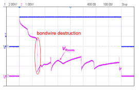
Figure 9: Dynamic behaviour after fusing of the bondwire.

To amplify the voltage $V_{\text{Kelvin}}$ sensed by the probes (see Fig. 7), a high-gain stage (AD8253 PGA) with gain $\in\,\{1,10,100,1000\}$ is combined with an integrated circuit (AD8250) whose gain $\in\,\{1,2,5,10\}$. All power transistors have their sources connected to a single sensing resistance of $1\,\mathrm{\Omega}\,(50\,\mathrm{W})$ that measures the voltage drop $V_{\text{Rsens}}$ inasmuch as the dominant current will always come from the branch of the active bondwire, while contributions from the other wires are negligible. Additionally a ringing snubber is added to compensate overshoots created by switching of an inductive load. The time evolution of $V_{\text{Kelvin}}$ and $V_{\text{Rsens}}$ is monitored with the oscilloscope (see Fig. 8). In parallel to the outputs $V_{\text{Rsens}}$ and $V_{\text{Kelvin}}$, Zener diodes (voltage limiters) are used to avoid damage of the external A/D converter when used in a sensitive range.

In Fig. 9 we show a selected screenshot of a fusing event that does not translate immediately into an open circuit. Various degradation processes have been identified with the delayed time-base features of the oscilloscope.

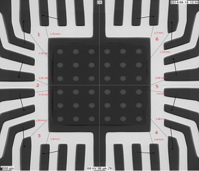
Figure 10: Example of an X-ray picture of a single package.

In Fig. 10 we show an X-ray picture of a sample package. Each sample package consists of 6 pairs of bondwires as enumerated in the picture. The length of each (in $\mathrm{mm}$) is also indicated therein. A fusing event is induced by using a long duration pulse. The characteristics of the pulse are controlled by the power supply Manson (capable of delivering up to $60\,\mathrm{A}$ at $16\,\mathrm{V}$) in order to obtain certain amount of current flowing through the bondwire. The time required to fuse the bondwire is measured and the results are then provided for all available types, that is material, diameter, and position within the package.

IV-D Optimisation Results

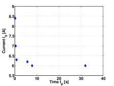
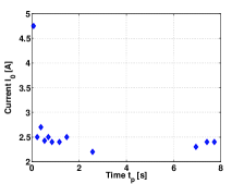
In this section we apply the afore-described parameter sub-set identification method to carry out the optimisation of the bondwire model. As stated before, each bondwire sample within a package (see Fig. 10) is characterised by a set of data points representing fusing events. Each fusing event corresponds to a pair $\{I_{0,i},t_{\text{p},i}\}$ representing the current amplitude $I_{0,i}$ that for given time $t_{\text{p},i}$ fuses the wire. In total 1077 bondwire samples within their package were deliberately fused in the data collection phase. Each data set is then filtered by means of a histogram to generate a sequence of smoother pairs $\{\bar{I}_{0,i},\bar{t}_{\text{p},i}\}$ that are used in the optimisation. Fig. 11 shows two examples of the resulting filtered data $\{\bar{I}_{0,i},\bar{t}_{\text{p},i}\}$ for $\mathrm{Au}$- and $\mathrm{Cu}$-wires of diameters $1.0\,\mathrm{mil}$ and $2.0\,\mathrm{mil}$ at position 1 in the package (see Fig. 10).

(a)

(b)

Figure 11: Experimental filtered data $\{\bar{I}_{0,i},\bar{t}_{\text{p},i}\}$ for gold and copper bondwires at position 1 in a package. (a) $\mathrm{Au}$-wire of $L_{\text{w}}=1.712\,\mathrm{mm}$ and $D_{\text{w}}=1.0\,\mathrm{mil}$; (b) $\mathrm{Cu}$-wire of $L_{\text{w}}=3.450\,\mathrm{mm}$ and $D_{\text{w}}=2.0\,\mathrm{mil}$.

Similar data is obtained for the bondwires at the other positions within the package. In Table. I and II, we collect the nominal geometric, electric, and thermic values of the bondwires. The nominal diameter $\bar{D}_{\text{w}}$ were provided by the package manufacturer, while the nominal length $\bar{L}_{\text{w}}$ has been obtained through averaging of the length measured via the x-ray scanning (see Fig. 10) and the length inferred from the lead-frame data-sheet.

TABLE I: Geometric characteristics of the bondwires within a package. The nominal $\bar{D}_{\text{w}}$ and $\bar{L}_{\text{w}}$ are given in $\mathrm{[mil]}$ and $\mathrm{[mm]}$.

	$\mathbf{Cu}$-wire			$\mathbf{Au}$-wire	Pos
	$1.0\,\mathrm{mil}$	$1.3\,\mathrm{mil}$	$2.0\,\mathrm{mil}$	$1.0\,\mathrm{mil}$
$\bar{L}_{\text{w}}$  $\mathrm{[mm]}$	$2.025\,\mathrm{}$	$3.445\,\mathrm{}$	$3.450\,\mathrm{}$	$1.712\,\mathrm{}$	$1$
	$1.267\,\mathrm{}$	$2.160\,\mathrm{}$	$2.160\,\mathrm{}$	$1.226\,\mathrm{}$	$2$
	$1.696\,\mathrm{}$	$3.458\,\mathrm{}$	$3.458\,\mathrm{}$	$1.889\,\mathrm{}$	$3$
	$1.670\,\mathrm{}$	$3.469\,\mathrm{}$	$3.469\,\mathrm{}$	$1.938\,\mathrm{}$	$4$
	$1.114\,\mathrm{}$	$2.126\,\mathrm{}$	$2.126\,\mathrm{}$	$1.369\,\mathrm{}$	$5$
	$1.884\,\mathrm{}$	$3.434\,\mathrm{}$	$3.434\,\mathrm{}$	$1.827\,\mathrm{}$	$6$

TABLE II: Nominal electric and thermic characteristics of the bondwires.

Elec	$\mathbf{Cu}$-wire	$\mathbf{Au}$-wire
$\bar{\uprho}_{\text{e;o}}\mathrm{[\Omega.m]}$	$1.678.10^{-8}$	$2.214.10^{-8}$
$\bar{\alpha}_{\uprho}\mathrm{[\frac{1}{K}]}$	$3.862.10^{-3}$	$3.400.10^{-3}$
Therm
$\bar{\rho}_{\text{w}}\mathrm{[\frac{Kg}{m^{3}}]}$	$8960$	$19300$
$\bar{\kappa}_{\text{o}}\mathrm{[\frac{W}{(m.K)}]}$	$398$	$315$
$\bar{\alpha}_{\kappa}\mathrm{[\frac{1}{K}]}$	$-4.675.10^{-4}$	$-2.744.10^{-4}$
$\bar{c}_{\text{e;w}}\mathrm{[\frac{J}{Kg.K}]}$	$353$	$129$
$\bar{\epsilon}_{\text{w}}$	$3.750.10^{-2}$	$2.475.10^{-1}$
$\bar{T}_{\text{ch}}\mathrm{[K]}$	$300.5$	$300.5$
$\bar{T}_{\text{ld}}\mathrm{[K]}$	$300.5$	$300.5$

The electric and thermic values collected in Table II are standard for these materials [16]. In particular, the value adopted for the emissivity $\bar{\epsilon}_{\text{w}}$ corresponds to polished copper and gold wires; nevertheless, for bondwires that are embedded in real packages, this polishness might not be the case. These values, together with the filtered data $\{\bar{I}_{0,i},\bar{t}_{\text{p},i}\}$, are substituted in (29)–(30) whence the well-posed parameters are established as explained above. In carrying out the optimisation of these parameters, we have adhered to the following principles stemming from the physicality of the problem.

• The bondwire length $L_{\text{w}}$ and diameter $D_{\text{w}}$ are always allowed to vary up to $30\%$ around their nominal values. This relative variation is the add up of the manufacturing tolerance, the tolerance in the x-ray scanning, the tolerance in the data-sheet, and a margin of safety.

• The chip and lead temperatures $T_{\text{ch}}$ and $T_{\text{ld}}$, although fixed as isothermal boundary conditions within the model, are allowed to vary up to $50\%$ above their nominal values. This is done to accommodate for the actual temperature increase these two bodies may undergo during a fusing event. This increase of temperature is certainly not negligible for fusing events characterised by long times to fuse.

• The dimensions of the moulding compound section around a bondwire at a given position, as required by the model, are directly taken from the package dimensions.

• The convective coefficient $h_{\text{c}}$ is assumed to be for air at normal conditions given that no special fluid dynamic condition in the room was expected.

• The remaining parameters are allowed to vary freely in a interval that makes physical sense, e.g., the emissivity is such that $0<\epsilon_{\text{w}}\leq 1$, while $\alpha_{\uprho}\geq 0$ and $\alpha_{\kappa}\leq 0$.

TABLE III: Overall average variation after optimisation of the parameters defining the bondwire model.

Geom	$\mathbf{Cu}$-wire			$\mathbf{Au}$-wire	$\mathbf{\Delta}_{\text{tot}}$
	$1.0\,\mathrm{mil}$	$1.3\,\mathrm{mil}$	$2.0\,\mathrm{mil}$	$1.0\,\mathrm{mil}$
$\Delta\bar{D}_{\text{w}}$	$-17.53\%$	$5.88\%$	$-20.39\%$	$-26.98\%$	$\mathbf{-14.76}\%$
$\Delta\bar{L}_{\text{w}}$	$12.88\%$	$-16.06\%$	$20.33\%$	$-3.92\%$	$\mathbf{3.31}\%$
Elec
$\Delta\bar{\uprho}_{\text{e;o}}$	$106.63\%$	$7.22\%$	$2.95\%$	$-18.54\%$	$\mathbf{24.57}\%$
$\Delta\bar{\alpha}_{\uprho}$	$-48.17\%$	$1.05\%$	$-21.07\%$	$-18.75\%$	$\mathbf{-21.74}\%$
Therm
$\Delta\bar{\rho}_{\text{w}}$	$144.43\%$	$142.44\%$	$341.53\%$	$181.43\%$	$\mathbf{202.46}\%$
$\Delta\bar{\kappa}_{\text{o}}$	$16.91\%$	$0.00\%$	$-15.00\%$	$-20.83\%$	$\mathbf{-4.73}\%$
$\Delta\bar{\alpha}_{\kappa}$	$36.42\%$	$-22.64\%$	$-322.67\%$	$-23.85\%$	$\mathbf{-83.19}\%$
$\Delta\bar{c}_{\text{e;w}}$	$126.04\%$	$298.23\%$	$125.96\%$	$187.63\%$	$\mathbf{184.47}\%$
$\Delta\bar{\epsilon}_{\text{w}}$	$390.81\%$	$-32.48\%$	$168.22\%$	$12.99\%$	$\mathbf{134.89}\%$
$\Delta\bar{T}_{\text{ch}}$	$19.73\%$	$10.00\%$	$24.17\%$	$30.00\%$	$\mathbf{20.98}\%$
$\Delta\bar{T}_{\text{ld}}$	$30.82\%$	$18.33\%$	$34.17\%$	$35.83\%$	$\mathbf{29.79}\%$

TABLE IV: Nominal electric and thermic characteristics of the bondwires within the package.

	$\mathbf{Cu}$-wire			$\mathbf{Au}$-wire	$\boldsymbol{\upvarepsilon}_{\text{tot}}$
	$1.0\,\mathrm{mil}$	$1.3\,\mathrm{mil}$	$2.0\,\mathrm{mil}$	$1.0\,\mathrm{mil}$
$\upvarepsilon^{\text{t}}_{\mathrm{B_{\text{w}}}}$	$31.52\%$	$21.70\%$	$27.83\%$	$35.87\%$	$\mathbf{29.23}\%$
$\upvarepsilon^{\text{s}}_{\mathrm{B_{\text{w}}}}$	$19.78\%$	$24.31\%$	$12.88\%$	$24.22\%$	$\mathbf{20.30}\%$
$\upvarepsilon^{\star\text{t}}_{\mathrm{B_{\text{w}}}}$	$6.95\%$	$3.26\%$	$3.26\%$	$8.81\%$	$\mathbf{5.57}\%$
$\upvarepsilon^{\star\text{s}}_{\mathrm{B_{\text{w}}}}$	$3.90\%$	$4.88\%$	$2.14\%$	$11.16\%$	$\mathbf{5.52}\%$

In Table III we have collected the average relative variation, with respect to their nominal values, of the parameters defining the bondwire model after optimisation. The variations are the average for each bondwire regardless of its position within the package. The overall total variation is given in the last column of the table. As we may see, all parameters undergo variations because the set of well-posed parameters, i.e., the parameters to be optimised, can be different from one data set to the other. Consequently, the parameters that are optimised for a bondwire at a given position may become the ill-posed ones for the bondwire at the next position.

As to the actual values of the variations, we first notice that the geometric parameters of the wire; namely its diameter and length, do not suffer major changes with respect to their nominal values. This implies that the model retains the physicality of the problem in this respect. Next, we start by recalling that the bondwire temperature formula in (16) consist of two distinguishable components; the first $\tilde{\theta}_{\text{w};2}(y)$ that accounts for the steady regime of the temperature, and second $\tilde{\theta}_{\text{w};1}(y,t)$ that gives account of the transient. By inspection of the corresponding formulas, we may identify which parameters play predominant roles in either regime. For instance, the parameters $\{\rho_{\text{w}},c_{\text{e;w}}\}$ have only influence on the transient (cf. (7)), whereas $\{\kappa_{\text{o}},\alpha_{\kappa},\uprho_{\text{e};\text{w}},\alpha_{\uprho},T_{\text{ch}},T_{\text{ld}}\}$ have mostly influence on the steady regime. Owing to the simplified configuration of the model and the dynamics of these two regimes in a real package, we may expect the model to yield better temperature estimations in the steady regime than in the transient. This fact manifest in the relatively high variation of $\{\rho_{\text{w}},c_{\text{e;w}}\}$ with respect to their nominal values as compared with the variation of $\{\kappa_{\text{o}},\alpha_{\kappa},\uprho_{\text{e};\text{w}},\alpha_{\uprho},T_{\text{ch}},T_{\text{ld}}\}$. With regard to the wire emissivity $\epsilon_{\text{w}}$, the overall high relative increase confirms that the assumption of polished wires is not a good initial guess.

To report on the accuracy of the model before and after optimisation, in Table IV we collect the average relative error of the model. The error therein is the average of the normalised residual (cf. (20)) for all bondwires regardless of their position within the package. We have split the error into the component $\upvarepsilon^{\text{t}}_{\mathrm{B_{\text{w}}}}$ that quantifies the error in the transient, and the component $\upvarepsilon^{\text{s}}_{\mathrm{B_{\text{w}}}}$ that does so in the steady regime. This splitting can be done by noticing in (16) that any fusing event occurring at a time less or equal than the relevant time constant is likely in the transient. The results in Table IV confirms what has been already inferred from Table III, that is the model yields better estimations for long time excitations. In general, the performance of the model before optimisation is pretty good, and is greatly improved with the optimisation.

V Conclusion

We have presented an extended analytic formula for the estimation of the heating of bondwires within real packages. The model retains the the shape and dimensions of the moulding compound surrounding the wire and imposes suitable boundary conditions for the temperature distribution. To yield the temperature along the wire, the model couples the heat transfer equations of both the wire and the compound by means of effective transfer coefficients that stems from the linearisation of the thermal radiation term on the wire surface. The resulting wire temperature formula consists of simple basic functions that make it suitable for a fast implementation into a numerical calculator. The model has also been optimised with a series of experimental measurements representing fusing events. The idea upon which the formula is built can be certainly extended to handle several bondwires in a package. This would entail defining as many effective transfer coefficients as bondwires.

Appendix A Moulding Compound Temperature Functions and Heat Kernel

Here, the functions comprising the compound temperature expression of (18) are derived. The component $\widetilde{T}_{\text{m}}\left(x,y,z,t\right)=\widetilde{T}_{\text{m};1}\left(x,y,z,t\right)+\widetilde{T}_{\text{m};2;1}\left(x,y,z\right)+\widetilde{T}_{\text{m};2;2}\left(x,y,z\right)$ must satisfy

$$\rho_{\text{m}}c_{\text{e};\text{m}}\frac{\partial\widetilde{T}_{\text{m}}}{\partial t}=\kappa_{\text{m}}\nabla^{2}\widetilde{T}_{\text{m}}.$$ (31)

Owing to their definition and the $yz$-plane of symmetry in Fig. 2, these components are subject to the following BCs

$$-\kappa_{\text{m}}\frac{\partial}{\partial z}\widetilde{T}_{\text{m};1}\left(x,y,\frac{H_{\text{m}}}{2},t\right)=h_{\text{c}}\widetilde{T}_{\text{m};1}\left(x,y,\frac{H_{\text{m}}}{2},t\right);$$

$$-\kappa_{\text{m}}\frac{\partial}{\partial z}\widetilde{T}_{\text{m};2,1}\left(x,y,\frac{H_{\text{m}}}{2}\right)=h_{\text{c}}\widetilde{T}_{\text{m};2,1}\left(x,y,\frac{H_{\text{m}}}{2}\right);$$ (32)

$$-\kappa_{\text{m}}\frac{\partial}{\partial z}\widetilde{T}_{\text{m};2,2}\left(x,y,\frac{H_{\text{m}}}{2}\right)=h_{\text{c}}\widetilde{T}_{\text{m};2,2}\left(x,y,\frac{H_{\text{m}}}{2}\right);$$

$$-\kappa_{\text{m}}\frac{\partial}{\partial x}\widetilde{T}_{\text{m};1}\left(\frac{W_{\text{m}}}{2},y,z,t\right)=h_{\text{c}}\widetilde{T}_{\text{m};1}\left(\frac{W_{\text{m}}}{2},y,z,t\right);$$

$$-\kappa_{\text{m}}\frac{\partial}{\partial x}\widetilde{T}_{\text{m};2,1}\left(\frac{W_{\text{m}}}{2},y,z\right)=h_{\text{c}}\widetilde{T}_{\text{m};2,1}\left(\frac{W_{\text{m}}}{2},y,z\right);$$ (33)

$$-\kappa_{\text{m}}\frac{\partial}{\partial x}\widetilde{T}_{\text{m};2,2}\left(\frac{W_{\text{m}}}{2},y,z\right)=h_{\text{c}}\widetilde{T}_{\text{m};2,2}\left(\frac{W_{\text{m}}}{2},y,z\right);$$

$$\widetilde{T}_{\text{m};1}\left(x,0,z,t\right) =0; \,-\kappa_{\text{m}}\frac{\partial}{\partial y}\widetilde{T}_{\text{m};1}\left(x,L_{\text{w}},z,t\right) =0;$$

$$\widetilde{T}_{\text{m};2,1}\left(x,0,z\right) =T_{\text{ch}}-T_{0}; \;-\kappa_{\text{m}}\frac{\partial}{\partial y}\widetilde{T}_{\text{m};2,1}\left(x,L_{\text{w}},z\right) =0;$$ (34)

$$\widetilde{T}_{\text{m};2,2}\left(x,0,z\right) =0; \;-\kappa_{\text{m}}\frac{\partial}{\partial y}\widetilde{T}_{\text{m};2,2}\left(x,L_{\text{w}},z\right) =0;$$

$$\frac{\partial}{\partial x}\widetilde{T}_{\text{m};1}\left(0,y,z,t\right) =0; \;\widetilde{T}_{\text{m};1}\left(x,y,-\frac{H_{\text{m}}}{2},t\right) =0;$$

$$\frac{\partial}{\partial x}\widetilde{T}_{\text{m};2,1}\left(0,y,z\right) =0; \;\widetilde{T}_{\text{m};2,1}\left(x,y,-\frac{H_{\text{m}}}{2}\right) =0;$$ (35)

$$\frac{\partial}{\partial x}\widetilde{T}_{\text{m};2,2}\left(0,y,z\right) =0; \;\widetilde{T}_{\text{m};2,2}\left(x,y,-\frac{H_{\text{m}}}{2}\right) =T_{\text{d}}-T_{0}.$$

Thus, by applying the method of separation of variables, we arrive at

$$\widetilde{T}_{\text{m};1}\!=\!\sum_{n}\sum_{m}\sum_{p}C^{\text{t}}_{\text{m};n,m,p}e^{-\frac{\kappa_{\text{m}}}{\rho_{\text{m}}c_{\text{e};\text{m}}}\left(\lambda^{2}_{x;\text{m},n}+\lambda^{2}_{y;\text{m},m}+\lambda^{2}_{z;\text{m},p}\right)t}\\ \cos\left(\lambda_{x;\text{m},n}x\right)\sin\left(\lambda_{y;\text{m},m}y\right)\sin\left(\lambda_{z;\text{m},p}\left(z+\frac{H_{\text{m}}}{2}\right)\right),$$ (36)

$$\widetilde{T}_{\text{m};2,1}\!=\!\sum_{n}\sum_{p}C^{\text{s}}_{\text{m};1;n,p}e^{\lambda_{y;\text{m};n,p}y}\left(1+e^{2\lambda_{y;\text{m};n,p}\left(L_{\text{w}}-y\right)}\right)\\ \cos\left(\lambda_{x;\text{m},n}x\right)\sin\left(\lambda_{z;\text{m},p}\left(z+\frac{H_{\text{m}}}{2}\right)\right),$$ (37)

$$\widetilde{T}_{\text{m};2,2}\!=\!\sum_{n}\sum_{m}C^{\text{s}}_{\text{m};2;n,m}\left(\!e^{\lambda_{z;\text{m};n,m}z}\!+\!\frac{\left(h_{\text{c}}+\kappa_{\text{m}}\lambda_{z;\text{m};n,m}\right)}{\left(\kappa_{\text{m}}\lambda_{z;\text{m};n,m}-h_{\text{c}}\right)}\right.\\ \left.e^{-\lambda_{z;\text{m};n,m}\left(z-H_{\text{m}}\right)}\right)\cos\left(\lambda_{x;\text{m},n}x\right)\sin\left(\lambda_{y;\text{m},m}y\right),$$ (38)

where $\lambda_{x;\text{m},n}$, $\lambda_{y;\text{m},m}$, and $\lambda_{z;\text{m},p}$ are solutions of the characteristic equations

$$\lambda_{x;\text{m},n}\tan\left(\lambda_{x;\text{m},n}\frac{W_{\text{m}}}{2}\right) =\!\frac{h_{\text{c}}}{\kappa_{\text{m}}}, \;\lambda_{z;\text{m},p}\cot\left(\lambda_{z;\text{m},p}H_{\text{m}}\right) =\!-\frac{h_{\text{c}}}{\kappa_{\text{m}}},$$

$$\lambda_{y;\text{m},m}=\frac{\left(2m+1\right)\pi}{2L_{\text{w}}},\;m\geq 0;$$ (39)

whereas $\lambda_{y;\text{m},n,p}$, and $\lambda_{z;\text{m},n,m}$ are given by

$$\lambda^{2}_{y;\text{m},n,p} =\lambda^{2}_{x;\text{m},n}+\lambda^{2}_{z;\text{m},p}, \;\lambda^{2}_{z;\text{m},n,m} =\lambda^{2}_{x;\text{m},n}+\lambda^{2}_{y;\text{m},m}.$$ (40)

Finally, the coefficients $\left\{C^{\text{t}}_{\text{m};n,m,p},C^{\text{s}}_{\text{m};1;n,p},C^{\text{s}}_{\text{m};2;n,m}\right\}$ are determined by the initial condition at $t=0$ and the relevant BCs in (34) and (35).

The compound heat kernel $G_{\text{m}}$ is calculated similarly. That is, we define $\widetilde{G}_{\text{m}}\equiv G_{\text{m}}-T_{0}$, and expand $\widetilde{G}_{\text{m}}=\widetilde{G}_{\text{m};1}+\widetilde{G}_{\text{m};2,1}+\widetilde{G}_{\text{m};2,2}$, and thus by recalling that $G_{\text{m}}$ for $t>0$ satisfies

$$\rho_{\text{m}}c_{\text{e;m}}\frac{\partial}{\partial t}G_{\text{m}}\left(x,y,z,t,y^{\prime}\right)=\kappa_{\text{m}}\nabla^{2}G_{\text{m}}\left(x,y,z,t,y^{\prime}\right),$$ (41)

it is not difficult to realise that the components $\widetilde{G}_{\text{m};1}$, $\widetilde{G}_{\text{m};2,1}$, and $\widetilde{G}_{\text{m};2,2}$ adopt expressions similar to those in (36)–(38) with coefficients $\left\{C^{\text{t}}_{\text{g};n,m,p},C^{\text{s}}_{\text{g};1;n,p},C^{\text{s}}_{\text{g};2;n,m}\right\}$, respectively. These coefficients are also obtained as before; for instance, $C^{\text{s}}_{\text{g};1;n,p}$ and $C^{\text{s}}_{\text{g};2;n,m}$ are obtained by replacing $T_{\text{ch}}-T_{0}$ and $T_{\text{d}}-T_{0}$ with $-T_{0}$ in the corresponding BCs of (34) and (35), while the transient coefficient $C^{\text{t}}_{\text{g};n,m,p}$ is obtained by considering (41) around $t=0$ where the impulse source $\dot{q}_{\text{i}}=\delta(x)\delta(y-y^{\prime})\delta(z)\delta(t)$ is defined. Therefore, it is the constant $C^{\text{t}}_{\text{g};n,m,p}$ that carries the dependence on $y^{\prime}$ associated with the Green’s function.

Appendix B Determination of the Model Auxiliary Constants

The constants $\widetilde{T}_{\text{w;e}}$ and $\chi_{\text{w}}$ are introduced in the model as consequence of the adopted linearisation. Strictly speaking, the actual wire effective temperature is the average of the wire exact temperature distribution. In the model, however, this value has become an auxiliary source term together with the wire-compound effective heat transfer coefficient $\chi_{\text{w}}$.

For starters, we realise that these auxiliary two constants do not allow us, as inferred from (16) and (18), to impose rigorously $T_{\text{w}}=T_{\text{m}};\,\forall y,\,\forall t$ at the common interface (see Fig. 2), and yet by introducing them, we facilitate accounting for the thermal interaction between the compound and the wire. Having said this, we are still allowed to state

$$\int\limits_{0}^{t_{\text{p}}}\int\limits_{0}^{L_{\text{w}}}\lim_{z\rightarrow 0}\lim_{x\rightarrow 0}\widetilde{T}_{\text{m}}\left(x,y,z,t\right)\mathrm{d}y\mathrm{d}t=\int\limits_{0}^{t_{\text{p}}}\int\limits_{0}^{L_{\text{w}}}\widetilde{T}_{\text{w}}\left(y,t\right)\mathrm{d}y\mathrm{d}t.$$ (42)

along the wire-compound interface. Such a condition holds true always, and it enables us to set an equation for computing $\widetilde{T}_{\text{w;e}}$ and $\chi_{\text{w}}$ in an iterative manner. Namely, at start we compute an effective wire temperature $\widetilde{T}^{(0)}_{\text{w;e}}$ as if there were no compound. Subsequently, a value $\chi^{(0)}_{\text{w}}$ is obtained from (42) by plugging $\widetilde{T}^{(0)}_{\text{w;e}}$ in (16) and (18); these two initial values of the constants are used to compute a new effective temperature $\widetilde{T}^{(1)}_{\text{w;e}}$ from (16), which in turn is used to derive $\chi^{(1)}_{\text{w}}$ from (42) again. This procedure is repeated until the pair $\{\widetilde{T}^{(i)}_{\text{w;e}},\chi^{(i)}_{\text{w}}\}$ stabilises. An important observation to keep in mind during the iterations is that the following constraint should hold true for every computed pair $\{\widetilde{T}^{(i)}_{\text{w;e}},\chi^{(i)}_{\text{w}}\}$

$$\widetilde{T}^{(i)}_{\text{w;e}}<\frac{2I^{2}_{0}\uprho_{\text{e;0}}\alpha_{\uprho}}{\epsilon_{\text{w}}\upsigma\chi^{(i)}_{\text{w}}A_{\text{w}}C_{\text{w}}\lvert\alpha_{\kappa}\rvert}.$$ (43)

This inequality stems from the very definition of these auxiliary constants and is readily obtained from (15).

References

• [1] G. T. Nöbauer and H. Moser, “Analytical Approach to Temperature Evaluation in Bonding Wires and Calculation of Allowable Current,” IEEE Trans. Adv. Packag., vol. 23, pp. 426–435, Aug 2000.
• [2] E. Loh, “Physical Analysis of Data of Fused-Open Bond Wires,” IEEE Trans. Comp., Hybrids, Manufact. Technol., vol. 6, pp. 209–217, Jun 1983.
• [3] A. Mertol, “Estimation of Aluminum and Gold Bond Wire Fusing Current and Fusing Time,” IEEE Trans. Comp., Hybrids, Manufact. Technol., vol. 18, pp. 210–214, Feb 1995.
• [4] E. Loh, “Heat Transfer of Fine-Wire Fuse,” IEEE Trans. Comp., Hybrids, Manufact. Technol., vol. 7, pp. 264–267, Sept 1984.
• [5] A. Mallik and R. Stout, “Simulation Methods for Predicting Fusing Current and Time for Encapsulated Wire Bonds,” IEEE Trans. Electron. Packag. Manufact., vol. 33, pp. 255–261, Oct 2010.
• [6] C. C. Jung, C. Silber, and J. Scheible, “Heat generation in bond wires,” IEEE Trans. Comp., Packag., Manufact. Technol. A, vol. 5, pp. 1465–1476, Oct 2015.
• [7] F. Incropera and D. DeWitt, Introduction to Heat Transfer.   Wiley, 1985.
• [8] J. Stewart, Vector Calculus, Calculus: Early Transcendentals.   Thompson Brooks/Cole, 2008.
• [9] W. Rudin, Functional Analysis.   McGraw-Hill, 1991.
• [10] S. Bayin, Mathematical Methods in Science and Engineering.   Wiley, 2006.
• [11] K. E. Atkinson, An Introduction to Numerical Analysis.   Wiley, 1989.
• [12] M. Velez-Reyes and G. C. Verghese, “Subset selection in identification, and application to speed and parameter estimation for induction machines,” in Proceedings of International Conference on Control Applications, Sep 1995, pp. 991–997.
• [13] M. Burth, G. C. Verghese, and M. Velez-Reyes, “Subset selection for improved parameter estimation in on-line identification of a synchronous generator,” IEEE Trans. Power Syst., vol. 14, no. 1, pp. 218–225, Feb 1999.
• [14] M. Fink, A. Attarian, and H. Tran, “Subset selection for parameter estimation in an hiv model,” PAMM, vol. 7, no. 1, pp. 1 121 501–1 121 502, 2007.
• [15] D. W. Lewis, Matrix Theory.   World Scientific, 1991.
• [16] The engineering toolbox. [Online]. Available: http://www.engineeringtoolbox.com