High-energy resummation in heavy-quark pair photoproduction

F.G. Celiberto^1,2†, D.Yu. Ivanov^3,4¶, B. Murdaca^2† and A. Papa^1,2†

¹ Dipartimento di Fisica, Università della Calabria

I-87036 Arcavacata di Rende, Cosenza, Italy

¹Istituto Nazionale di Fisica Nucleare, Gruppo collegato di Cosenza

I-87036 Arcavacata di Rende, Cosenza, Italy

³ Sobolev Institute of Mathematics, 630090 Novosibirsk, Russia

⁴ Novosibirsk State University, 630090 Novosibirsk, Russia

We present our predictions for the inclusive production of two heavy quark-antiquark pairs, separated by a large rapidity interval, in the collision of (quasi-)real photons at the energies of LEP2 and of some future electron-positron colliders. We include in our calculation the full resummation of leading logarithms in the center-of-mass energy and a partial resummation of the next-to-leading logarithms, within the Balitsky-Fadin-Kuraev-Lipatov (BFKL) approach.

^†e-mail: francescogiovanni.celiberto, beatrice.murdaca, alessandro.papa  @fis.unical.it

^¶e-mail: d-ivanov@math.nsc.ru

1 Introduction

The high energies reached at the LHC and in possible future hadron and electron-positron colliders represent a great chance in the search for long-waited signals of New Physics. They offer, however, also a unique opportunity to test the Standard Model in unprecedented kinematic ranges. A vast class of processes can be studied at high-energy colliders, called semihard processes, characterized by a clear hierarchy of scales, $s\gg Q^{2}\gg\Lambda_{\rm QCD}^{2}$, where $s$ is the squared center-of-mass energy, $Q$ is the hard scale given by the process kinematics and $\Lambda_{\rm QCD}$ is the QCD mass scale, which still represent a challenge for QCD in the high-energy limit. Here the fixed-order perturbative description, allowed by the presence of a hard energy scale, misses the effect of large energy logarithms, which compensate the smallness of the coupling $\alpha_{s}$ and must therefore be resummed to all orders. The theoretical framework for this resummation is provided by the Balitsky–Fadin–Kuraev–Lipatov (BFKL) approach [1], whereby a systematic procedure has become available for resumming all terms proportional to $(\alpha_{s}\ln(s))^{n}$, the so called leading logarithmic approximation (LLA), and also those proportional to $\alpha_{s}(\alpha_{s}\ln(s))^{n}$, the so called next-to-leading approximation (NLA). In both cases, within the BFKL approach, the (possibly differential) cross section of processes falling in the domain of perturbative QCD, takes a peculiar factorized form, whose ingredients are the impact factors describing the transition from each colliding particle to the respective final state object, and a process-independent Green’s function. The BFKL Green’s function obeys an integral equation, whose kernel is known at the next-to-leading order (NLO) both for forward scattering (i.e. for $t=0$ and color singlet in the $t$-channel) [2, 3] and for any fixed (not growing with energy) momentum transfer $t$ and any possible two-gluon color state in the $t$-channel [4, 5, 6].

The phenomenological reach of the BFKL approach is limited by the number of available impact factors. So far, only a few of them have been calculated with next-to-leading order accuracy: i) impact factors for colliding quarks and gluons [7, 8, 9, 10], which are at the basis of the calculation of the ii) forward jet impact factors (or jet vertices) in exact form [11, 12, 13] or in the small-cone approximations [14, 15] and of the iii) forward hadron impact factors [16], iv) impact factor for the $\gamma^{*}$ to light vector meson transition at leading twist [17], v) impact factor for the $\gamma^{*}$ to $\gamma^{*}$ transition [18, 19].

Jet vertices have extensively been used to produce with NLA accuracy a number of predictions [20, 21, 23, 22, 25, 24, 26, 27, 28, 29, 30, 31, 32] for the Mueller-Navelet jet production process at the LHC, resulting in nice agreement with experimental determinations [33]. The same vertices enter the calculation of several observables in the inclusive production of three and four jets, separated in rapidity, at the LHC [34, 35, 36, 37, 38].

The forward hadron impact factors were recently used to calculate the cross section and some azimuthal correlations in the inclusive production of two identified hadrons composed of light quarks and separated in rapidity [39, 40] which could also be studied at the LHC.

The impact factor for the $\gamma^{*}$ to light vector meson transition enters the imaginary part of the cross section for the exclusive production of two light vector mesons in the collision of two highly virtual photons [41, 42, 43, 44, 45], which could be considered in future linear colliders.

The $\gamma^{*}$ to $\gamma^{*}$ impact factor is the ingredient for the $\gamma^{*}\gamma^{*}$ total cross section, which is considered to be the gold-plated channel for the manifestation of the BFKL dynamics. A number of predictions for this cross section were built, with partial inclusion of NLA BFKL effects [46, 47, 48, 49] and with full NLA accuracy [50, 51], whose comparison with the only available data from LEP2 cannot be conclusive due to the relatively small center-of-mass energy and the limiting accuracy of LEP2 experiment.

In this paper we introduce another process which could serve as a probe of BFKL dynamics: the inclusive production of two heavy quark-antiquark pairs, separated in rapidity, in the collision of two real (or quasi-real) photons,

$$\gamma(p_{1})+\gamma(p_{2})\longrightarrow Q(q_{1})\ +X\ +Q(q_{2})\;,$$ (1)

where $Q$ here stands for a charm/bottom quark or antiquark. In Fig. 1 we present a schematic representation of this process, in the case when the tagged objects are a heavy quark with momentum $q_{1}$, detected in the fragmentation region of the photon with momentum $p_{1}$, and a heavy quark with momentum $q_{2}$, detected in the fragmentation region of the photon with momentum $p_{2}$. This process can be studied either at electron-positron or in nucleus-nucleus colliders via collisions of two quasi-real photons. In this first exploratory study, we will focus on the case of electron-positron colliders and will adopt the equivalent photon approximation (EPA) to parametrize the photon flux emitted by the colliding electrons and positrons. The main aim is to show that sensible predictions can be built, within the BFKL approach with NLA, which can be compared with experimental results. For the sake of definiteness, we will consider the center-of-mass energies of LEP2 and of the CLIC future collider.

The totally inclusive two heavy-quark pair production process has much in common with the above discussed inclusive interaction of two virtual photons (the $\gamma^{*}\gamma^{*}$ total cross section). Here the large values of masses of the produced heavy quarks play the role of hard scale, similar to the role that large photon virtualities play in $\gamma^{*}\gamma^{*}$ interactions. It is interesting to note that just this observable, the total inclusive cross section for two heavy-quark pairs photoproduction, was calculated first in QCD within BFKL resummation method, see the paper by I. Balitsky and L. Lipatov in [1]. Despite the fact that the BFKL resummation gives formally a finite result for this total cross section, it does not represent an observable that can be directly confronted with the experiment. Indeed, in order to be sure that two heavy-quark pairs are produced in the event, one needs to detect at least one of the heavy quarks in each quark pair. The other reason for the tagging of two heavy quarks is that the knowledge of their momenta (their rapidities) allows one to keep control on the energy of the collision of two quasi-real photons in $e^{+}e^{-}$ experiments. In our present study we restrict/fix the momenta of these two tagged quarks as if they were true final states. As a further step, one needs to include into the theoretical analysis the heavy-quark fragmentation describing the tagging procedure of heavy quarks in the particular experiment.

An attractive idea is to consider also similar experiments which assume the detection of the pair of heavy quarks, separated by a large rapidity interval, in photon-photon interactions via ultra-peripheral (UPC) nucleus-nucleus collisions at the LHC. In [52] the total cross section for the production of two heavy-quark pairs in such collisions was estimated in the LO BFKL approach at a sizeable value. However the kinematics of experiments with a tagged pair of heavy quarks separated by the rapidity interval of a few units requires rather large energies of the colliding quasi-real photons. Unfortunately at the LHC the energies of such photon-photon interactions in the UPC heavy nucleus-nucleus collisions fall in the kinematic range where the quasi-real photon fluxes from the colliding heavy nuclei are greatly suppressed due to electromagnetic nuclear form factors, and therefore such experiments look not feasible.

The paper is organized as follows: in Section 2 we explain the theoretical setup of our calculation; in Section 3 we present our results for the cross sections azimuthal angle correlations in dependence on the rapidity interval between the tagged heavy quarks; in Section 4 we discuss our results and draw conclusions.

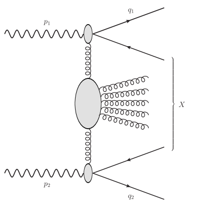
Figure 1: Diagrammatic representation of the heavy-quark pair photoproduction in the case when a heavy quark with transverse momentum $q_{1}$ ($q_{2}$) from the upper (lower) vertex is tagged.

2 Theoretical setup

For the process under consideration, given in Eq. (1), we plan to construct the cross section, differential in some of the kinematic variables of the tagged heavy quark or antiquark, and some azimuthal correlations between the tagged fermions. In the BFKL approach the cross section takes a factorized form, schematically represented in Fig. 2, given by the convolution of the impact factors for the transition from a (quasi-)real photon to a heavy quark-antiquark pair (the upper and lower ovals in Fig. 2, labeled by $\Phi$) with the BFKL Green’s function $G$. The crosses in Fig. 2 denote the tagged quarks, whose momenta are not integrated over in getting the expression for the cross section.

In our calculation we will partially include NLA resummation effects, by taking the BFKL Green’s function in the NLA, while keeping the impact factors at the leading order, since their next-to-leading order corrections are not yet known.

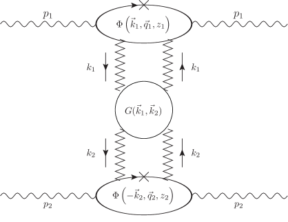
Figure 2: Schematic representation of the BFKL factorization for the process under consideration.

2.1 The impact factor

The (differential) impact factor for the photoproduction of a heavy quark pair reads

$$d{\Phi}=\frac{\alpha\alpha_{s}e_{Q}^{2}}{\pi}\left[m^{2}R^{2}+\vec{P}^{2}\left(z^{2}+\overline{z}^{2}\right)\right]d^{2}q\ dz\,,$$ (2)

where $R$ and $\vec{P}$ read

$$R=\frac{1}{m^{2}+\vec{q}^{\,\,2}}-\frac{1}{m^{2}+(\vec{q}-\vec{k})^{2}}\;,\;\;\;\;\;\vec{P}=\frac{\vec{q}}{m^{2}+\vec{q}^{\,\,2}}+\frac{\vec{k}-\vec{q}}{m^{2}+(\vec{q}-\vec{k})^{2}}\,.$$ (3)

Here $\alpha$ and $\alpha_{s}$ denote the QED and QCD couplings, $e_{Q}$ denotes the electric charge of the heavy quark, $m$ stands for the heavy-quark mass, $z$ and ${\overline{z}}\equiv 1-z$ are the longitudinal fractions of the quark and antiquark produced in the same vertex and $\vec{k}$, $\vec{q}$, $\vec{k}-\vec{q}$ represent the transverse momenta with respect to the photons collision axis of the Reggeized gluon, the produced quark and antiquark, respectively. The details of the derivation of this result may be found, for instance, in [53]. Such impact factor differs only by the coupling and overall normalization from the similar QED quantity known since long and used in the calculations of the lepton-pair production.

In the following we will need the projection of the impact factors onto the eigenfunctions of the leading-order BFKL kernel, to get their so called $\left(n,\nu\right)$-representation. We get

$$v_{R^{2}}\equiv\int\frac{d^{2}k}{\pi\sqrt{2}}\left(k^{2}\right)^{i\nu-3/2}e^{in\vartheta}R^{2}$$

$$=\frac{1}{\sqrt{2}}\frac{\Gamma\left(\frac{1}{2}+\frac{n}{2}-i\nu\right)\Gamma\left(\frac{1}{2}+\frac{n}{2}+i\nu\right)\left(\vec{q}^{\,\,2}\right)^{\frac{n}{2}}e^{in\varphi}\left(\frac{1}{2}+\frac{n}{2}-i\nu\right)}{\Gamma\left(n+1\right)\left(m^{2}+\vec{q}^{\,\,2}\right)^{\frac{5}{2}+\frac{n}{2}-i\nu}\left(\frac{n}{2}+i\nu-\frac{1}{2}\right)}$$

$$\times\left[\left(\frac{3}{2}+\frac{n}{2}-i\nu\right)\,_{2}F_{1}\left(\frac{n}{2}-\frac{1}{2}+i\nu,\,\frac{5}{2}+\frac{n}{2}-i\nu,\,1+n,\,\zeta\right)\right.$$

$$-\left.2\,_{2}F_{1}\left(\frac{n}{2}-\frac{1}{2}+i\nu,\,\frac{3}{2}+\frac{n}{2}-i\nu,\,1+n,\,\zeta\right)\right]$$ (4)

$$\equiv e^{in\varphi}\,c_{R^{2}}(n,\nu,\vec{q}^{\>2})$$

and

$$v_{\vec{P}^{\,2}}\equiv\int\frac{d^{2}k}{\pi\sqrt{2}}\left(k^{2}\right)^{i\nu-3/2}e^{in\vartheta}\vec{P}^{\,2}$$

$$=\frac{1}{\sqrt{2}}\frac{\Gamma\left(\frac{1}{2}+\frac{n}{2}-i\nu\right)\Gamma\left(\frac{1}{2}+\frac{n}{2}+i\nu\right)\left(\vec{q}^{\,\,2}\right)^{\frac{n}{2}}e^{in\varphi}\left(\frac{1}{2}+\frac{n}{2}-i\nu\right)}{\Gamma\left(1+n\right)\left(m^{2}+\vec{q}^{\,\,2}\right)^{\frac{3}{2}+\frac{n}{2}-i\nu}\left(-\frac{1}{2}+\frac{n}{2}+i\nu\right)}$$

$$\times\left\{\,\left[1+2i\nu\,(1-\zeta)\right]{{}_{2}}F_{1}\left(\frac{n}{2}-\frac{1}{2}+i\nu,\,\frac{3}{2}+\frac{n}{2}-i\nu,\,1+n,\,\zeta\right)\right.$$

$$+\left.\frac{\nu^{2}-i\nu+\frac{3}{4}+\frac{n^{2}}{4}}{i\nu-\frac{1}{2}-\frac{n}{2}}\,{{}_{2}}F_{1}\left(\frac{n}{2}-\frac{1}{2}+i\nu,\,\frac{1}{2}+\frac{n}{2}-i\nu,\,1+n,\,\zeta\right)\right\}$$ (5)

$$\equiv e^{in\varphi}\,c_{\vec{P}^{\,2}}(n,\nu,\vec{q}^{\>2})\;,$$

where $\zeta\equiv\frac{\vec{q}^{\,\,2}}{m^{2}+\vec{q}^{\,\,2}}$; the azimuthal angles $\vartheta$ and $\varphi$ are defined as $\cos\vartheta\equiv k_{x}/|\vec{k}|$ and $\cos\varphi\equiv q_{x}/|\vec{q}|$.

2.2 Kinematics of the process

For the tagged quark momenta we introduce the standard Sudakov decomposition, using as light-cone basis the momenta $p_{1}$ and $p_{2}$ of the colliding photons,

$$q=zp_{1}+\frac{m^{2}+\vec{q}^{\,\,2}}{zW^{2}}p_{2}+q_{\perp}\,,$$ (6)

with $W^{2}=\left(p_{1}+p_{2}\right)^{2}=2p_{1}p_{2}=4E_{\gamma_{1}}E_{\gamma_{2}}$; $p_{1}=\frac{E_{\gamma_{1}}}{2}\left(1,\vec{0},1\right)$ and $p_{2}=\frac{E_{\gamma_{2}}}{2}\left(1,\vec{0},-1\right)$, so that

$$2qp_{2}=W^{2}z=2E_{\gamma_{2}}\left(E+q_{\parallel}\right)\ ,$$

$$2qp_{1}=\frac{m^{2}+\vec{q}^{\,\,2}}{z}=2E_{\gamma_{1}}\left(E-q_{\parallel}\right)\;;$$

here $q=\left(E,\vec{q},q_{\parallel}\right)$ and the rapidity can be expressed as

$$y=\frac{1}{2}\ln\frac{E+q_{\parallel}}{E-q_{\parallel}}=\ln\frac{2E_{\gamma_{1}}z}{\sqrt{m^{2}+\vec{q}^{\,\,2}}}\;.$$

Therefore for the rapidities of the two tagged quarks in our process we have

$$y_{1}=\ln\frac{2E_{\gamma_{1}}z_{1}}{\sqrt{m^{2}+\vec{q}_{1}^{\,\,2}}}\;\;\;\text{and}\;\;\;y_{2}=-\ln\frac{2E_{\gamma_{2}}z_{2}}{\sqrt{m^{2}+\vec{q}_{2}^{\,\,2}}}\;,$$

whence their rapidity difference is

$$\Delta Y\equiv y_{1}-y_{2}=\ln\frac{W^{2}z_{1}z_{2}}{\sqrt{\left(m^{2}+\vec{q}_{1}^{\,\,2}\right)\left(m^{2}+\vec{q}_{2}^{\,\,2}\right)}}\;.$$

For the semihard kinematic we have the requirement

$$\frac{W^{2}}{\sqrt{\left(m^{2}+\vec{q}_{1}^{\,\,2}\right)\left(m^{2}+\vec{q}_{2}^{\,\,2}\right)}}=\frac{e^{\Delta Y}}{z_{1}z_{2}}\gg 1\;,$$

therefore we will consider the kinematic when $\Delta Y\geq\Delta_{0}\sim 1\div 2$.

In what follows we will need a cross section differential in the rapidities of the tagged quarks, therefore we have to make the following change of variables:

$$z_{1}\to y_{1}=\ln\frac{2E_{\gamma_{1}}z_{1}}{\sqrt{m^{2}+\vec{q}_{1}^{\,\,2}}}\;,\;\;\;dy_{1}=\frac{dz_{1}}{z_{1}}\;,$$

$$z_{2}\to y_{2}=-\ln\frac{2E_{\gamma_{2}}z_{2}}{\sqrt{m^{2}+\vec{q}_{2}^{\,\,2}}}\;,\;\;\;dy_{2}=-\frac{dz_{2}}{z_{2}}\;,$$

which implies

$$dz_{1}dz_{2}=\frac{e^{y_{1}-y_{2}}\sqrt{m^{2}+\vec{q}^{\,\,2}_{1}}\sqrt{m^{2}+\vec{q}^{\,\,2}_{2}}}{W^{2}}dy_{1}dy_{2}\;.$$

2.2.1 The BFKL cross section and azimuthal coefficients

Similarly to the Mueller-Navelet jet and the dihadron production processes (see Refs. [23, 40]), the differential cross section for the inclusive production of a pair of heavy quarks separated in rapidity (a “diquark” system in what follows) can be cast in the following form:

$$\frac{d\sigma}{dy_{1}dy_{2}d|\vec{q}_{1}|d|\vec{q}_{2}|d\phi_{1}d\phi_{2}}=\frac{1}{(2\pi)^{2}}\left[{\cal C}_{0}+2\sum_{n=1}^{\infty}\cos(n\varphi){\cal C}_{n}\right]\;,$$

where $\varphi=\varphi_{1}-\varphi_{2}-\pi$, while ${\cal C}_{0}$ gives the cross section averaged over the azimuthal angles $\varphi_{1,2}$ of the produced quarks and the other coefficients ${\cal C}_{n}$ determine the distribution of the relative azimuthal angle between the two quarks.

The expression for the ${\cal C}_{n}$ coefficient is the following ($q_{1,2}\equiv|\vec{q}_{1,2}|$):

$${\cal C}_{n}=\frac{q_{1}q_{2}\,\sqrt{m_{1}^{2}+q^{2}_{1}}\sqrt{m_{2}^{2}+q^{2}_{2}}}{W^{2}}e^{\Delta Y}$$

$$\times\int d\nu\left(\frac{W^{2}}{s_{0}}\right)^{{\overline{\alpha}_{s}}\left(\mu_{R}\right)\chi\left(n,\nu\right)+\overline{\alpha}_{s}^{2}\left(\mu_{R}\right)\left(\bar{\chi}\left(n,\nu\right)+\frac{\beta_{0}}{8N_{c}}\chi\left(n,\nu\right)\left(-\chi\left(n,\nu\right)+\frac{10}{3}+2\ln\frac{\mu_{R}^{2}}{\sqrt{s_{1}s_{2}}}\right)\right)}$$

$$\times\alpha_{s}^{2}\left(\mu_{R}\right)c_{1}(n,\nu,\vec{q}_{1}^{\>2},z_{1})c_{2}(n,\nu,\vec{q}_{2}^{\>2},z_{2})$$

$$\times\left\{1+{\overline{\alpha}_{s}}\left(\mu_{R}\right)\left(\frac{\bar{c}_{1}^{(1)}}{c_{1}}+\frac{\bar{c}_{2}^{(1)}}{c_{2}}\right)+{\overline{\alpha}_{s}}\left(\mu_{R}\right)\frac{\beta_{0}}{2N_{c}}\left(\frac{5}{3}+\ln\frac{\mu_{R}^{2}}{s_{1}s_{2}}+f\left(\nu\right)\right)\right.$$

$$\left.+\overline{\alpha}_{s}^{2}(\mu_{R})\,\ln\left({\frac{W^{2}}{s_{0}}}\right)\,\frac{\beta_{0}}{4N_{c}}\,\chi\left(n,\nu\right)f(\nu)\right\}\;,$$ (7)

where

$$\chi\left(n,\nu\right)=2\psi\left(1\right)-\psi\left(\frac{n}{2}+\frac{1}{2}+i\nu\right)-\psi\left(\frac{n}{2}+\frac{1}{2}-i\nu\right)$$

are the eigenvalues of the leading-order BFKL kernel, with $\psi(x)=\Gamma^{\prime}(x)/\Gamma(x)$, and

$$\beta_{0}=\frac{11}{3}N_{c}-\frac{2}{3}n_{f}$$

is the first coefficient of the QCD $\beta$-function, responsible for running-coupling effects. The function $f\left(\nu\right)$ is defined by

$$i\frac{d}{d\nu}\ln\frac{c_{1}}{c_{2}}=2\left[f\left(\nu\right)-\ln\left(\sqrt{s_{1}s_{2}}\right)\right]\;,$$

with $s_{i}$, $i=1,2$ being the hard scales in our two-tagged-quark process, which we chose equal to $m_{i}^{2}+\vec{q}_{i}^{\>2}$ , and

$$c_{1}(n,\nu,\vec{q}_{1}^{\>2},z_{1})=\frac{\alpha e_{Q_{1}}^{2}}{\pi}\left[m_{1}^{2}c_{R^{2}}(n,\nu,\vec{q}_{1}^{\>2})+\left(z_{1}^{2}+\overline{z}_{1}^{2}\right)c_{\vec{P}^{2}}(n,\nu,\vec{q}_{1}^{\>2})\right]\;,$$

$$c_{2}(n,\nu,\vec{q}_{2}^{\>2},z_{2})=\frac{\alpha e_{Q_{2}}^{2}}{\pi}\left[m_{2}^{2}c^{*}_{R^{2}}(n,\nu,\vec{q}_{2}^{\>2})+\left(z_{2}^{2}+\overline{z}_{2}^{2}\right)c^{*}_{\vec{P}^{2}}(n,\nu,\vec{q}_{2}^{\>2})\right]\;,$$

$$\frac{\bar{c}_{1}^{(1)}}{c_{1}}+\frac{\bar{c}_{2}^{(1)}}{c_{2}}=\chi\left(n,\nu\right)\ln\frac{s_{0}}{\sqrt{\left(m_{1}^{2}+\vec{q}^{\,\,2}_{1}\right)\left(m_{2}^{2}+\vec{q}^{\,\,2}_{2}\right)}}\;.$$

The scale $s_{0}$ can be arbitrarily chosen, within NLA accuracy; in our calculation we made the choice $s_{0}=\sqrt{s_{1}s_{2}}$. Equation (7) is written for the general case when two heavy quarks of different flavors with masses $m_{1}$ and $m_{2}$ are detected.

2.3 The $e^{+}e^{-}$ cross section

To pass from the photon-initiated process to the one initiated by $e^{+}e^{-}$ collisions, we must take into account the flux of quasi-real photons $dn$ emitted by each of the two colliding particles,

$$d\sigma_{e^{+}e^{-}}=dn_{1}dn_{2}d\sigma_{\gamma\gamma}\;,$$

with

$$dn=\frac{\alpha}{\pi}\frac{dx}{x}\left[1-x+\frac{x^{2}}{2}-\frac{m_{e}^{2}\left(1-x\right)x^{2}}{\vec{q}^{\,\,2}+m_{e}^{2}x^{2}}\right]\frac{d\vec{q}^{\,\,2}}{\vec{q}^{\,\,2}+m_{e}^{2}x^{2}}\;,$$ (8)

where $x=\frac{\omega}{E_{e}}$ is the fraction of the electron (positron) energy carried by the photon and $\vec{q}$ denotes now the transverse component of the photon momentum. The emission angle is $\theta\approx\frac{q_{\perp}}{E_{e}\left(1-x\right)}$ and we will consider the antitag experiment, so that $\theta\leq\theta_{0}$ whence $(\vec{q})_{\rm max}=E_{e}\left(1-x\right)\theta_{0}$.

Integrating in Eq. (8) over $\vec{q}^{\,\,2}$, we get

$$dn=\frac{\alpha}{\pi}\frac{dx}{x}\left[\left(1-x+\frac{x^{2}}{2}\right)\ln\left(\frac{E_{e}^{2}\theta_{0}^{2}\left(1-x\right)^{2}+m_{e}^{2}x^{2}}{m_{e}^{2}x^{2}}\right)-(1-x)\right]\;,$$

where some terms ${\cal O}(m_{e}^{2}/E_{e}^{2})$ were neglected.

Therefore the general expression for our observables is

$$\frac{d\sigma_{e^{+}e^{-}}}{d\left(\Delta Y\right)}=\int dq_{1}\int dq_{2}\int_{-y_{\rm max}^{(1)}}^{y_{\rm max}^{(1)}}dy_{1}\int_{-y_{\rm max}^{(2)}}^{y_{\rm max}^{(2)}}dy_{2}\,\delta\left(y_{1}-y_{2}-\Delta Y\right)$$

$$\times\int_{e^{-\left(y_{\rm max}^{(1)}-y_{1}\right)}}^{1}\frac{dn_{1}}{dx_{1}}dx_{1}\int_{e^{-\left(y_{\rm max}^{(2)}+y_{2}\right)}}^{1}\frac{dn_{2}}{dx_{2}}dx_{2}\,d\sigma_{\gamma\gamma}\;,$$ (9)

with $y_{\rm max}^{(1)}=\ln\sqrt{\frac{s}{m_{1}^{2}+\vec{q}^{\,\,2}_{1}}}$ and $y_{\rm max}^{(2)}=\ln\sqrt{\frac{s}{m_{2}^{2}+\vec{q}^{\,\,2}_{2}}}$.

In order to give predictions to be confronted with experiment, we have to integrate our fully differential cross section over some range of the tagged quarks transverse momenta. In what follows we label such integrated coefficients with $C_{n}$.

2.4 The “box” $q\bar{q}$ cross section

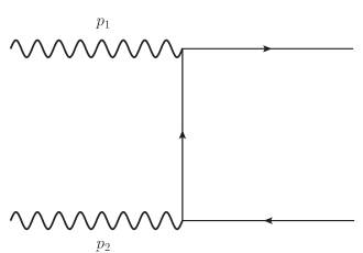
Figure 3: One of the two Feynman diagrams contributing at the lowest order to the $q\bar{q}$ photoproduction. The other one is the diagram with crossed fermionic lines.

As a background contribution for the case when a quark and an antiquark of the same flavor are detected, we have to consider the lowest-order QED cross section for the production of a heavy quark and antiquark in photon-photon collisions. In our notations the corresponding $e^{+}e^{-}$ cross section reads

$$\frac{d\sigma_{ee}}{d(\Delta Y)}=\int_{0}^{\frac{s_{ee}}{2(1+\cosh(\Delta Y))}-m^{2}}\frac{dq^{2}}{(m^{2}+q^{2})^{2}}\frac{2\pi\alpha^{2}e_{q}^{4}N_{c}}{\left(1+\cosh(\Delta Y)\right)^{2}}$$

$$\times\left[\frac{\cosh(\Delta Y)}{2}+\frac{m^{2}}{m^{2}+q^{2}}-\left(\frac{m^{2}}{m^{2}+q^{2}}\right)^{2}\right]$$

$$\times\left(\frac{\alpha}{\pi}\right)^{2}\left[f(y)\left(\ln\left(\frac{\Lambda^{2}}{m_{e}^{2}y}\right)-1\right)^{2}-\frac{1}{3}\left(\ln\frac{1}{y}\right)^{3}\right]\;,$$ (10)

where

$$y=\frac{w^{2}}{s_{ee}}=\frac{2\left(1+\cosh(\Delta Y)\right)\left(m^{2}+q^{2}\right)}{s_{ee}}\;,$$

with

$$f(y)=\left(1+\frac{y}{2}\right)^{2}\ln\frac{1}{y}-\frac{1}{2}\left(1-y\right)\left(3+y\right)$$

and $\Lambda\simeq m^{2}$.

In the case when the heavy quarks of different flavor, two quarks or two antiquark of the same flavor, are detected, the “box” mechanism does not represent, of course, a background channel.

3 Numerical analysis

3.1 Results

In this Section we present our results for the dependence on the rapidity separation between the two tagged quarks, $\Delta Y=y_{1}-y_{2}$, of the $\varphi$-averaged cross section $C_{0}$ and of the ratios $R_{10}\equiv C_{1}/{C}_{0}$ and $R_{20}\equiv C_{2}/{C}_{0}$ ratios. We consider here only the case of charm quark and fix the mass $m$ at the value 1.2 GeV/$c^{2}$.

Introducing some reasonable kinematic cuts, we integrate the quark transverse momenta in the symmetric range $q_{\rm min}<q_{1,2}<q_{\rm max}$. We fix $q_{\rm max}$ to 10 GeV and consider below the three cases $q_{\rm min}=0$, 1, 3 GeV. We fix the center-of-mass energy to $\sqrt{s}=200$ GeV, typical of LEP2 analyses, and study the behavior of our observables in the rapidity range $1<\Delta Y<6$. For comparison, we give predictions of $C_{0}$ and $R_{10}$ also at $\sqrt{s}=3$ TeV, characteristic of the future $e^{+}e^{-}$ CLIC linear accelerator. In the last case, we allow for a larger rapidity interval between the two quarks, i.e. $1<\Delta Y<11$. We fix the maximum for the lepton emission angle $\theta_{0}=0.0835$, which is inside of the acceptance range of the OPAL forward detectors [54, 55]. All calculations are done in the $\overline{\rm MS}$ scheme.

Pure LLA and NLA BFKL predictions, together with the “box” $q\bar{q}$ calculation of $C_{0}$ for $q_{\rm min}=0$ GeV and $\sqrt{s}=200$ GeV, are shown respectively in Table 1 and 2.

Results for $C_{0}$, $R_{10}$, and $R_{20}$ for $q_{\rm min}=1$, 3 GeV and $\sqrt{s}=200$ GeV are shown in Fig. 4. For comparison, predictions for $C_{0}$ and $R_{10}$ for $q_{\rm min}=1$, 3 GeV and $\sqrt{s}=3$ TeV are shown in Fig. 5.

Table 1: $\Delta Y$-dependence of the $\varphi$-averaged cross section $C_{0}$ [pb] for $q_{\rm min}=0$ GeV and $\sqrt{s}=200$ GeV. LLA and NLA predictions are compared with the “box” $q\bar{q}$ cross section. $C$ stands for $\mu_{R}^{2}/(s_{1}s_{2})$.

$\Delta Y$	Box $q\bar{q}$	$\begin{array}[]{c}\rm LLA\\ C=1/2\end{array}$	$\begin{array}[]{c}\rm LLA\\ C=1\end{array}$	$\begin{array}[]{c}\rm LLA\\ C=2\end{array}$	$\begin{array}[]{c}\rm NLA\\ C=1/2\end{array}$	$\begin{array}[]{c}\rm NLA\\ C=1\end{array}$	$\begin{array}[]{c}\rm NLA\\ C=2\end{array}$
1.5	98.26	51.87(17)	8.155(39)	3.618(18)	2.120(13)	1.4046(91)	1.2861(93)
2.5	42.73	90.46(26)	11.080(44)	4.322(21)	2.197(11)	1.1976(71)	1.0623(70)
3.5	14.077	150.42(43)	14.166(54)	4.876(20)	2.315(12)	0.9986(54)	0.8296(45)
4.5	3.9497	231.45(62)	16.705(65)	5.053(24)	2.301(11)	0.7763(39)	0.6116(32)
5.5	0.9862	319.93(89)	17.529(69)	4.648(21)	2.121(10)	0.5411(27)	0.3922(19)

Table 2: $\Delta Y$-dependence of the $\varphi$-averaged cross section $C_{0}$ [pb] for $q_{\rm min}=0$ GeV and $\sqrt{s}=3$ TeV. LLA and NLA predictions are compared with box $q\bar{q}$ cross section. $C$ stands for $\mu_{R}^{2}/(s_{1}s_{2})$.

$\Delta Y$	Box $q\bar{q}$	$\begin{array}[]{c}\rm LLA\\ C=1/2\end{array}$	$\begin{array}[]{c}\rm LLA\\ C=1\end{array}$	$\begin{array}[]{c}\rm LLA\\ C=2\end{array}$	$\begin{array}[]{c}\rm NLA\\ C=1/2\end{array}$	$\begin{array}[]{c}\rm NLA\\ C=1\end{array}$	$\begin{array}[]{c}\rm NLA\\ C=2\end{array}$
1.5	280.98	1361.6(6.1)	66.40(30)	24.44(11)	12.45(11)	7.292(72)	6.521(73)
3.5	48.93	6856(18)	196.12(95)	54.93(26)	23.07(14)	8.153(62)	6.798(59)
5.5	4.9819	31860(71)	551.2(2.4)	116.33(53)	47.53(23)	9.479(67)	6.903(45)
7.5	0.4318	130215(271)	1365.1(5.5)	217.9(1.0)	94.54(44)	10.243(56)	6.435(33)
9.5	0.0323	428626(977)	2691.2(9.9)	327.3(1.5)	158.38(76)	9.092(45)	4.858(24)
10.5	0.0081	683469(1833)	3278(13)	345.2(1.5)	180.42(90)	7.497(37)	3.651(18)

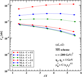
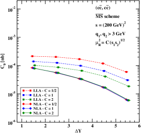
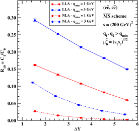
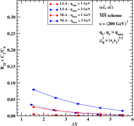
Figure 4: $\Delta Y$-dependence of $C_{0}$, $R_{10}$, and $R_{20}$ for $q_{\rm min}=1$, 3 GeV, $\sqrt{s}=200$ GeV, and for different values of $C=\mu_{R}^{2}/\sqrt{s_{1}s_{2}}$, with $s_{1,2}=m_{1,2}^{2}+q_{1,2}^{2}$. Data points have been slightly shifted along the horizontal axis for the sake of readability.

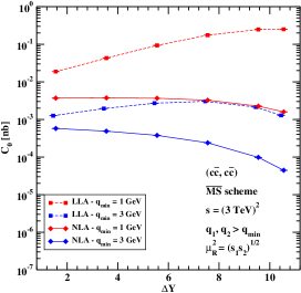
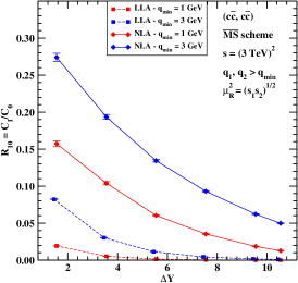
Figure 5: $\Delta Y$-dependence of $C_{0}$ and $R_{10}$ for $q_{\rm min}=1$, 3 GeV, $\sqrt{s}=3$ TeV, and for $\mu_{R}^{2}=\sqrt{s_{1}s_{2}}$, with $s_{1,2}=m_{1,2}^{2}+q_{1,2}^{2}$. Data points have been slightly shifted along the horizontal axis for the sake of readability.

3.2 Numerical tools and uncertainty estimation

All numerical calculations were done in Fortran. Numerical integrations were performed using routines implemented in the Cuba library [56, 57], making extensive use of the Monte Carlo Vegas [58] integrator. The numerical stability of our results was crosschecked by separate calculations performed using both Mathematica and the Dadmul CERNLIB routine [59].

The most important source of uncertainty comes from the numerical six-dimensional integration over the variables $|\vec{q}_{1}|$, $|\vec{q}_{2}|$, $y_{1}$, $\nu$, $x_{1}$, and $x_{2}$ and was directly estimated by the Vegas integration routine [58]. We checked that other sources of uncertainties, related with the upper cutoff in the integrations over $|\vec{q}_{1}|$, $|\vec{q}_{2}|$, and $\nu$, are negligible with respect to the first one. Thus, the error bars of all predictions are just those given by Vegas. The other, internal source of uncertainty of our calculation is related with the scale of the running QCD coupling. Below we quantify this uncertainty studying the renormalization scale dependence. We vary $\mu_{R}^{2}$ around its “natural” value $\sqrt{s_{1}s_{2}}$ in the range 1/2 to two. The parameter $C$ entering Tables 1 and 2 gives the ratio $\mu_{R}^{2}/\sqrt{s_{1}s_{2}}$.

3.3 Discussion

The inspection of results in Table 1 suggests that the cross section $C_{0}$ is smaller than the reference “box” cross section. This is similar to what occurred in the calculations of the total $\gamma^{*}\gamma^{*}$ cross section, where it was found that the “box” mechanism gives still a very important contribution at LEP2 energies. The situation changes if we pass to the larger energies and therefore larger rapidity differences that are possibly available at future $e^{+}e^{-}$ colliders. Here the BFKL mechanism with the gluonic exchange in the $t$-channel starts to win over the “box” one with the fermionic $t$-channel exchange, see our results in Table 2. We stress, however, that for our two heavy-quark (or two heavy-antiquark) tagged process, contrary to the $\gamma^{*}\gamma^{*}$ case, the “box” mechanism is not a background. The cross section exhibits the expected trends: it increases when moving from the LEP2 energies to the CLIC ones and decreases when moving from the LLA to the NLA, a typical feature in the BFKL approach. We note also that our partial inclusion of NLA effects leads to results that are less sensitive to the variation of the renormalization scale than the results of LLA BFKL resummation.

Azimuthal correlations are in all cases much smaller than one and decrease when $\Delta Y$ increases, as it must be due to the larger emission of undetected partons. The reason for this smallness, with respect to the case of Mueller-Navelet jets or di-hadron systems (see, e.g., Refs. [23, 40]) is that in this case there is not any kinematic constraint, even at the lowest order in perturbation theory, between the transverse momenta of the two tagged quarks, since they are produced in two different vertices (each of them together with an antiquark). When the minimum value of the tagged quark transverse momentum $q_{\rm min}$ is increased, azimuthal correlations increase due to the more limited available phase space in the transverse space and the consequently more constrained transverse kinematics. We can see that the inclusion of NLA effects increases the correlations, which can only be explained with the larger suppression of $C_{0}$ with respect to $C_{1,2}$ when these effects are included.

4 Summary and outlook

We have considered the inclusive photoproduction of two heavy quarks separated in rapidity, taking into account the resummation to all orders of the leading energy logarithms and the resummation of the next-to-leading ones entering the BFKL Green’s function. We have calculated the cross section for this process averaged over the relative azimuthal angle of the two tagged quarks and presented results for the azimuthal angle correlations, considering for definiteness the case in which photons are emitted by electron and positrons colliding at the energies of the LEP2 and the CLIC colliders.

The trends of our results with the energy of the collision beam and the behavior of the considered observables with the rapidity interval $\Delta Y$ between the tagged quarks is just as expected: azimuthal correlations decrease with increasing $\Delta Y$. Moreover, just as in the case of Mueller-Navelet jets and dihadron production, the inclusion of next-to-leading order correction reduces the decorrelation. In absolute value, azimuthal correlations are much smaller with respect to Mueller-Navelet jets and dihadrons, a result which is not surprising since here we have a two heavy-quark pair production mechanism and the two tagged quarks are produced in the leading order in different interaction vertices, having independent transverse momenta.

This process extends the list of semihard processes by which strong interactions in the high-energy limit, and in particular the BFKL resummation procedure, can be probed in the future $e^{+}e^{-}$ linear colliders.

There are several obvious developments of this work. One is the calculation of the next-to-leading order impact factor for the photoproduction of a heavy quark-antiquark pair, which would allow for the full NLA treatment of the process under consideration. The other is to include into the theoretical analysis heavy-quark fragmentation describing the experimental tagging procedure of heavy quarks.

As we already noted, the possibility for the experimental study of our process in UPC collisions of heavy ions at the LHC kinematics is not feasible, unfortunately. Nevertheless, the study of heavy-quark observables that reveal BFKL resummation effects looks promising in the LHC proton-proton collisions. Recently, in [60] the process of inclusive forward $J/\Psi$-meson and very backward jet production was suggested. The other interesting possibility is to extend the methods used in our work to the case of two detected heavy-quark inclusive hadroproduction, i.e. a process similar to the one considered here, but initiated by quarks and gluons emitted by protons (in collinear factorization) rather than by photons.

References

- [1] V.S. Fadin, E. Kuraev, L. Lipatov, Phys. Lett. B 60, 50 (1975); Sov. Phys. JETP 44, 443 (1976); E. Kuraev, L. Lipatov, V.S. Fadin, Sov. Phys. JETP 45, 199 (1977); I. Balitsky, L. Lipatov, Sov. J. Nucl. Phys. 28, 822 (1978).
- [2] V.S. Fadin, L.N. Lipatov, Phys. Lett. B 429 (1998) 127.
- [3] M. Ciafaloni, G. Camici, Phys. Lett. B 430 (1998) 349.
- [4] V.S. Fadin, R. Fiore, A. Papa, Phys. Rev. D 60 (1999) 074025.
- [5] V.S. Fadin, D.A. Gorbachev, Pisma v Zh. Eksp. Teor. Fiz. 71 (2000) 322 [JETP Letters 71 (2000) 222]; Phys. Atom. Nucl. 63 (2000) 2157 [Yad. Fiz. 63 (2000) 2253].
- [6] V.S. Fadin, R. Fiore, Phys. Lett. B610 (2005) 61 [Erratum-ibid. 621 (2005) 61]; Phys. Rev. D 72 (2005) 014018.
- [7] V.S. Fadin, R. Fiore, M.I. Kotsky, A. Papa, Phys. Lett. D61 (2000) 094005.
- [8] V.S. Fadin, R. Fiore, M.I. Kotsky, A. Papa, Phys. Lett. D61 (2000).
- [9] M. Ciafaloni and D. Colferai, Nucl. Phys. B 538 (1999) 187.
- [10] M. Ciafaloni and G. Rodrigo, JHEP 0005 (2000) 042.
- [11] J. Bartels, D. Colferai and G.P. Vacca, Eur. Phys. J. C 24 (2002) 83.
- [12] J. Bartels, D. Colferai and G.P. Vacca, Eur. Phys. J. C 29 (2003) 235.
- [13] F. Caporale, D.Yu. Ivanov, B. Murdaca, A. Papa and A. Perri, JHEP 1202, 101 (2012).
- [14] D.Yu. Ivanov, A. Papa, JHEP 1205, 086 (2012).
- [15] D. Colferai, A. Niccoli, JHEP 1504, 071 (2015).
- [16] D.Yu. Ivanov, A. Papa, JHEP 1207 (2012) 045.
- [17] D.Yu. Ivanov, M.I. Kotsky and A. Papa, Eur. Phys. J. C 38 (2004) 195.
- [18] J. Bartels, S. Gieseke and C. F. Qiao, Phys. Rev. D 63 (2001) 056014 [Erratum-ibid. D 65 (2002) 079902]; J. Bartels, S. Gieseke and A. Kyrieleis, Phys. Rev. D 65 (2002) 014006; J. Bartels, D. Colferai, S. Gieseke and A. Kyrieleis, Phys. Rev. D 66 (2002) 094017; J. Bartels, Nucl. Phys. (Proc. Suppl.) (2003) 116; J. Bartels and A. Kyrieleis, Phys. Rev. D 70 (2004) 114003; V.S. Fadin, D.Yu. Ivanov and M.I. Kotsky, Phys. Atom. Nucl. 65 (2002) 1513 [Yad. Fiz. 65 (2002) 1551]; Nucl. Phys. B 658 (2003) 156.
- [19] I. Balitsky, G.A. Chirilli, Phys. Rev. D 87 (2013) 014013.
- [20] D. Colferai, F. Schwennsen, L. Szymanowski, S. Wallon, JHEP 1012 (2010) 026.
- [21] M. Angioni, G. Chachamis, J.D. Madrigal, A. Sabio Vera, Phys. Rev. Lett. 107, 191601 (2011).
- [22] B. Ducloué, L. Szymanowski, S. Wallon, JHEP 1305 (2013) 096.
- [23] F. Caporale, D.Yu. Ivanov, B. Murdaca, A. Papa, Nucl. Phys. B 877 (2013) 73.
- [24] F. Caporale, B. Murdaca, A. Sabio Vera, C. Salas, Nucl. Phys. B 875 (2013) 134.
- [25] B. Ducloué, L. Szymanowski, S. Wallon, Phys. Rev. Lett. 112 (2014) 082003.
- [26] B. Ducloué, L. Szymanowski, S. Wallon, Phys. Lett. B 738 (2014) 311.
- [27] F. Caporale, D.Yu. Ivanov, B. Murdaca, A. Papa, Eur. Phys. J. C 74, no. 10, 3084 (2014) [Erratum-ibid. 75, no. 11, 535 (2015)].
- [28] B. Ducloué, L. Szymanowski and S. Wallon, Phys. Rev. D 92 (2015) no.7, 076002.
- [29] F. Caporale, D.Yu. Ivanov, B. Murdaca, A. Papa, Phys. Rev. D 91 (2015) no.11, 114009.
- [30] F.G. Celiberto, D.Yu. Ivanov, B. Murdaca, A. Papa, Eur. Phys. J. C 75 (2015) no.6, 292.
- [31] F.G. Celiberto, D.Yu. Ivanov, B. Murdaca, A. Papa, Eur. Phys. J. C 76 (2016) no.4, 224.
- [32] G. Chachamis, arXiv:1512.04430 [hep-ph].
- [33] V. Khachatryan et al. [CMS Collaboration], JHEP 1608 (2016) 139.
- [34] F. Caporale, G. Chachamis, B. Murdaca, A. Sabio Vera, Phys. Rev. Lett. 116 (2016) no.1, 012001 [arXiv:1508.07711 [hep-ph]].
- [35] F. Caporale, F.G. Celiberto, G. Chachamis, A. Sabio Vera, Eur. Phys. J. C 76 (2016) no.3, 165 [arXiv:1512.03364 [hep-ph]].
- [36] F. Caporale, F.G. Celiberto, G. Chachamis, D. Gordo G mez, A. Sabio Vera, Nucl. Phys. B 910 (2016) 374 [arXiv:1603.07785 [hep-ph]].
- [37] F. Caporale, F.G. Celiberto, G. Chachamis, D. Gordo G mez, A. Sabio Vera, Eur. Phys. J. C 77 (2017) no.1, 5 [arXiv:1606.00574 [hep-ph]].
- [38] F. Caporale, F.G. Celiberto, G. Chachamis, D. Gordo G mez, A. Sabio Vera, Phys. Rev. D 95 (2017) no.7, 074007 [arXiv:1612.05428 [hep-ph]].
- [39] F.G. Celiberto, D.Yu. Ivanov, B. Murdaca, A. Papa, Phys. Rev. D 94 (2016) no.3, 034013.
- [40] F.G. Celiberto, D.Yu. Ivanov, B. Murdaca, A. Papa, Eur. Phys. J. C 77 (2017) no.6, 382.
- [41] D.Yu. Ivanov and A. Papa, Nucl. Phys. B732 (2006) 183.
- [42] D.Yu. Ivanov and A. Papa, Eur. Phys. J. C49 (2007) 947.
- [43] M. Segond, L. Szymanowski and S. Wallon, Eur. Phys. J. C52 (2007) 93.
- [44] R. Enberg, B. Pire, L. Szymanowski and S. Wallon, Eur. Phys. J. C45 (2006) 759 [Erratum-ibid. C51 (2007) 1015].
- [45] B. Pire, L. Szymanowski and S. Wallon, Eur. Phys. J. C44 (2005) 545.
- [46] S.J. Brodsky, V.S. Fadin, V.T. Kim, L.N. Lipatov, G.B. Pivovarov, JETP Lett. 76 (2002) 249 [Pisma Zh. Eksp. Teor. Fiz. 76 (2002) 306].
- [47] S.J. Brodsky, V.S. Fadin, V.T. Kim, L.N. Lipatov, G.B. Pivovarov, JETP Lett. 70 (1999) 155.
- [48] F. Caporale, D.Yu. Ivanov, A. Papa, Eur. Phys. J. C 58 (2008) 1-7.
- [49] X.-C. Zheng, X.-G. Wu, S.-Q. Wang, J.-M. Shen, Q.-L. Zhang, JHEP 1310 (2013) 117.
- [50] G.A. Chirilli, Yu.V. Kovchegov, JHEP 1405 (2014) 099.
- [51] D.Yu. Ivanov, B. Murdaca, A. Papa, JHEP 1410 (2014) 058.
- [52] V.P. Goncalves and M.V.T. Machado, Eur. Phys. J. C 29 (2003) 37.
- [53] I.F. Ginzburg and D.Yu. Ivanov, Phys. Rev. D 54, 5523 (1996) [hep-ph/9604437].
- [54] K. Ahmet et al. [OPAL Collaboration], Nucl. Instrum. Meth. A 305 (1991) 275.
- [55] G. Abbiendi et al. [OPAL Collaboration], Phys. Lett. B 539 (2002) 13 [hep-ex/0206021].
- [56] T. Hahn, Comput. Phys. Commun. 168 (2005) 78 [arXiv:1408.6373 [hep-ph]].
- [57] T. Hahn, J. Phys. Conf. Ser. 608 (2015) 1 [arXiv:hep-ph/0404043].
- [58] G.P. Lepage, J. Comput. Phys. 27 (1978) 192.
- [59] CERNLIB Homepage: http://cernlib.web.cern.ch/cernlib
- [60] R. Boussarie, B. Duclou , L. Szymanowski and S. Wallon, arXiv:1709.01380 [hep-ph].