1 Equiangular nets in $\bbS^{2}$

We demonstrate that certain polyhedral cones are integrable, in the sense of Definition LABEL:def:integrable. First, we demonstrate that $\mathbf{Y}\times\mathbb{R}$ and $\mathbf{T}$ (under certain circumstances) admit no hole conditions.

1.1 No-holes for $\mathbf{Y}$ and $\mathbf{T}$

The $\mathbf{Y}^{1}\times\mathbb{R}^{m}$ cone is very special, in that closeness to thise cone always guarantees the existence of good density points. No extra assumptions on the class or structure of the varifold are necessary.

Proposition 1.1.

There is an $\varepsilon(m,k,\delta)$ so that if $M^{1+m}\subset\mathbb{R}^{1+k+m}$ lies in $M\in\mathcal{N}_{\varepsilon}(\mathbf{Y}\times\mathbb{R}^{m})$, then $M$ satisfies the $\delta$-no-holes condition in $B_{1/2}$ w.r.t. $\mathbf{Y}\times\mathbb{R}^{m}$.

Proof.

By Lemma LABEL:lem:global-graph, provided $\varepsilon$ is sufficiently small $M\cap B_{3/4}\setminus B_{\delta}({\{0\}\times\mathbb{R}^{m}})$ is a $C^{1,\alpha}$-perturbation of $\mathbf{Y}\times\mathbb{R}^{m}$. We claim that

$$\mathrm{sing}M\cap(\mathbb{R}^{1+k}\times\{y\})\cap B_{1/2}\neq\emptyset\quad\forall y\in B_{1/2}^{m}.$$ (1)

Otherwise, since $\mathrm{sing}M$ is relatively closed, by Sard’s theorem, we could choose a $y^{*}$ arbitrarily near $y$ so that $M\cap(\mathbb{R}^{1+k}\times\{y^{*}\})\cap B_{1/2}$ would consist of a smooth $1$-manifold having three boundary components, which is impossible.

Therefore, using Almgren’s stratification we have for $\mathcal{H}^{m}$-a.e. $y\in B_{1/2}^{m}$ a singular point $X_{y}\in\mathrm{sing}M\cap(B_{\delta}(0)^{1+k}\times\{y\})$ which is $m$-symmetric. So there is a tangent cone at $X_{y}$ which is either a multiplicity $\geq 2$ plane, or a union of $\geq 3$ half-planes, either of which has density $\geq\theta_{\mathbf{Y}}(0)$. ∎

Unfortunately, the tetrahedral cones $\mathbf{T}^{2}\times\mathbb{R}^{m}$ do not admit so nice a property, without imposing further restrictions: we can find piecewise-smooth varifolds of bounded mean curvature which look very close to $\mathbf{T}$ at scale $B_{1}$, but which only have singularities of type $\mathbf{Y}\times\mathbb{R}$. To rule this out one can enforce a boundary/orientability structure.

Lemma 1.2.

Let $\mathbf{C}=\mathbf{C}_{0}^{2}\times\mathbb{R}^{m}\subset\mathbb{R}^{3+m}$, where $\mathbf{C}_{0}$ is $2$-dimensional, stationary and singular. If (up to rotation) $\mathbf{C}_{0}$ is not a multiplicity $1$ plane or the $\mathbf{Y}\times\mathbb{R}$, then we have

$$\theta_{\mathbf{C}}(0)\geq\theta_{\mathbf{T}}(0).$$ (2)

Proof.

If $\mathbf{C}_{0}$ is planar, then it must be with multiplicity $\geq 2>\theta_{\mathbf{T}}(0)$. If $\mathbf{C}_{0}$ has $1$-degree of symmetry, then since we are not regular nor are we the $\mathbf{Y}$, then $\mathbf{C}_{0}$ must consist of $\geq 4$ half-planes meeting along an edge, which also has multplicity $\geq 2$.

Suppose $\mathbf{C}_{0}$ has no symmetries. Consider the geodesic net $\Gamma:=\mathbf{C}_{0}\cap\partial B_{1}\subset\bbS^{2}$. If any geodesic has multiplicity $\geq 2$, or any junction has $\geq 4$ vertices, then $\theta_{\mathbf{C}}(0)\geq 2$ and we are done. Let us suppose therefore that $\Gamma$ consists only of multiplicity-$1$ geodesics, which meet at $120^{\circ}$.

These nets are classified, and listed in the following subsection. One can readily verify that the net with least length, aside from the circle and $\mathbf{Y}$, is the tetrahedral net. ∎

Lemma 1.3.

Let $M^{2}$ be a set in $\mathbb{R}^{3}$ which coincides with $\mathbf{T}^{2}$ in $B_{1}\setminus B_{\delta}$. Suppose $\mathcal{H}^{2}\llcorner M$ is an integral varifold with an associated cycle structure in $B_{1}$. Then there is a point $x\in M\cap B_{1}$, so that $M$ near $x$ is not a $C^{1}$ perturbation of $\mathbb{R}^{2}$ or $\mathbf{Y}\times\mathbb{R}$.

Proof.

By assumption $M$ divides the annulus $B_{1}\setminus B_{\delta}$ into four regions $A_{1},A_{2},A_{3},A_{4}$. Any two $A_{i}$, $A_{j}$ share a boundary wedge $W\subset\mathbf{T}$.

Suppose, towards a contradiction, that around every point $M$ is locally a $C^{1}$ perturbation of $\mathbb{R}^{2}$ or $\mathbf{Y}\times\mathbb{R}$. Then $M\cap B_{1}$ consists of a finite collection of $C^{1}$ embedded surfaces $M_{i}$ meeting at $120^{\circ}$ along $C^{1}$ embedded curves $\gamma_{i}$. Since $M$ coincides with $\mathbf{T}$ outside $B_{\delta}$, we see that up to renumbering the curves $\gamma_{1}$, $\gamma_{2}$ start and end at vertices of $\mathbf{T}\cap S^{2}$, while curves $\gamma_{3},\gamma_{4},\ldots$ must be closed. See figure 1 for an idealized picture.

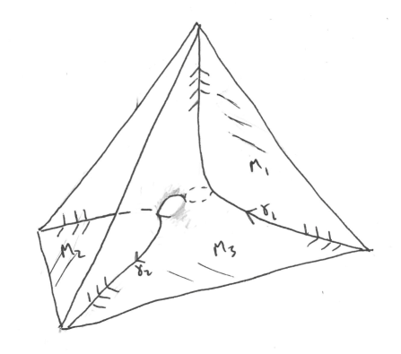
Figure 1: A surfaces with only $\mathbf{Y}$-type singularities which coincides with $\mathbf{T}$ outside a small ball.

We can assume $\gamma_{1}$ starts at the vertex adjoined by regions $A_{1},A_{2},A_{3}$, while $\gamma_{1}$ ends at the vertex adjoined by regions $A_{1},A_{2},A_{4}$. A small tubular neighborhood of $\gamma_{1}$ is diffeomorphic $\mathbf{Y}\times\mathbb{R}$, and therefore if we push $\gamma_{1}$ away from any bounding surface in the conormal direction, the resulting curve $\hat{\gamma}_{1}$ induces a path connecting $A_{i}$ ($i=1,2,3$) to some $A_{j}$ ($j=1,2,4$). After relabeling as necessary, we can thicken $\hat{\gamma}_{1}$ to obtain an open set $A$, disjoint from $M$, with $A\supset A_{3}\cup A_{4}$.

Since each associated current is codimension $1$ and without boundary, we can assume WLOG that $\mathcal{H}^{2}\llcorner M$ is associated to a countable union of boundaries $\partial[U_{i}]$, where $U_{i}$ are open sets, and we take the boundaries as $3$-currents. From the above we have $A\subset U_{i}$ or $A\cap U_{i}=\emptyset$ for every $i$. But now if $W$ is the boundary wedge shared by $A_{3},A_{4}$, then the previous sentence implies

$$W\cap(B_{1/2}\setminus B_{2\delta})\cap\mathrm{spt}\partial[U_{i}]=\emptyset\quad\forall i.$$ (3)

And so $W$ cannot be part of $M$. This is a contradiction. ∎

Remark 1.4.

If one could show either curve $\gamma_{1}$ or $\gamma_{2}$ is unknotted (as in Figure 1), then one could construct a Lipschitz deformation of $M$ onto two faces of the solid tetrahedron (plus one edge). This would prove Lemma 1.3 for general $(\mass,\varepsilon,\delta)$-sets (at least for $\varepsilon$ sufficiently small) without any extra orientation or codimension requirements. Unfortunately, we have very little idea whether Lemma 1.2 holds in general codimension.

Proposition 1.5.

There is an $\varepsilon(m,\delta)$ so that the following holds. Let $M^{n=2+m}\subset\mathbb{R}^{3+m}$ be an integral varifold with associated cycle structure in $B_{1}$, and suppose $M\in\mathcal{N}_{\varepsilon}(\mathbf{T}^{2}\times\mathbb{R}^{m})$. Then $M$ satisfies the $\delta$-no-holes condition in $B_{1/2}$.

Proof.

By Lemma LABEL:lem:poly-global-graph, $M\cap B_{3/4}\setminus B_{\delta}({\{0\}\times\mathbb{R}^{m}})$ is a $C^{1,\alpha}$-perturbation of $\mathbf{T}\times\mathbb{R}^{m}$, for $\varepsilon(m,\delta)$ sufficiently small. So

$$\mathrm{sing}M\cap B_{3/4}\subset B_{\delta}({\{0\}\times\mathbb{R}^{m}}),$$ (4)

and there is no loss in assuming $M\cap B_{3/4}\setminus B_{\delta}({\{0\}\times\mathbb{R}^{m}})$ coincides with $\mathbf{T}\times\mathbb{R}^{m}$.

We claim that, for every $y\in B_{1/2}^{m}$, there is some singular point

$$X_{y}\in\mathrm{sing}M\cap(\mathbb{R}^{3}\times\{y\})\cap B_{1/2}$$ (5)

which is not a (multiplicity-1) $\mathbf{Y}\times\mathbb{R}^{1+m}$. We prove this by contradiction.

First, observe that by Simon’s regularity Theorem LABEL:thm:Y-reg, the set of singular points which are not a multiplicity-1 $\mathbf{Y}\times\mathbb{R}^{1+m}$ is relatively closed in $\mathrm{sing}M$, and hence closed. Therefore, if the claim failed, it would fail for $y$ in some open set $U$. Using Allard’s and Simon’s regularity we obtain that $M\cap(\mathbb{R}^{3}\times U)$ consists of embedded, multiplicity-one $C^{1}$ $n$-surfaces, meeting at $120^{0}$ along embedded $C^{1}$ $(n-1)$-surfaces.

Therefore by Sard’s theorem, for a.e. $y\in U$, the $M\cap(\mathbb{R}^{3}\times\{y\})$ consists of embedded $C^{1}$ surfaces meeting at $120^{\circ}$ along embedded $C^{1}$ curves, which coincides with $\mathbf{T}^{2}$ in an annulus. However, by slicing we also have that for a.e. $y\in U$, $\mathcal{H}^{2}\llcorner M\cap(\mathbb{R}^{3}\times\{y\})$ has an associated cycle structure in $B_{1/4}(0,y)$, contradicting Lemma 1.3. This proves the claim.

The Proposition is completed by combining (4) and the above claim with Lemma 1.2. ∎

1.2 Integrability

We establish integrability of those polyhedral cones which arise from an equiangular geodesic net in $\bbS^{2}$. As discussed in Remark LABEL:rem:maybe-non-int, it seems possible to us that in higher-codimension there exist non-integrable polyhedral cones (for either definition of integrability). Indeed, even in the codimension-$1$ case we are unable to give a general abstract proof, but instead we make use of the classification of equiangular geodesics nets in $\bbS^{2}$ due to [lamarle], [heppes] and proceed on a case-by-case basis.

Theorem 1.6.

Suppose $\mathbf{C}^{2}\subset\mathbb{R}^{3}\subset\mathbb{R}^{2+k}$ is a polyhedral cone. Then $\mathbf{C}$ is integrable in $\mathbb{R}^{2+k}$. In particular the tetrahedron $\mathbf{T}^{2}\subset\mathbb{R}^{2+k}$ is integrable.

Proof.

Fix a polyhedral cone $\mathbf{C}^{2}\subset\mathbb{R}^{3}\subset\mathbb{R}^{2+k}$, composed of wedges $\cup_{i=1}^{d}W(i)$. Write $\Gamma=\mathbf{C}\cap\bbS^{1+k}$ for the corresponding equiangular geodesic net, and $\ell(i)\equiv W(i)\cap\bbS^{1+k}$ for the geodesic segments. After relabeling as necessary we can assume $\ell(1),\ell(2),\ell(3)$ share a common vertex.

Let $v:\mathbf{C}\to\mathbf{C}^{\perp}$ be a linear, compatible Jacobi field. We wish to show that $v=\pi_{\mathbf{C}^{\perp}}\circ A$ for some skew-symmetric matrix $A:\mathbb{R}^{2+k}\to\mathbb{R}^{2+k}$. From Proposition LABEL:prop:baby-linear we know this holds locally, in the sense that there is a skew-symmetric $A_{0}$, so that

$$v(i)=\pi_{\mathbf{C}^{\perp}}\circ A_{0}\quad i=1,2,3.$$ (6)

Therefore, by considering the field $v-\pi_{\mathbf{C}^{\perp}}\circ A_{0}$, we can and shall reduce to the case when $v(1)=v(2)=v(3)=0$.

In fact we shall prove that any linear, compatible Jacobi field $v$ satsifying $v(1)=v(2)=v(3)=0$ must be identically zero. It is reasonable to expect this to be true, as the $v(i)$s with their compatibility conditions effectively form a system of linear equations, and one can easily verify that the total number of variables equals the total number of conditions (equals $2kd$). However an abstract counting argument seems insufficient to establish $v\equiv 0$, as the linear independence of this system depends strongly on both the global topology and geometry of the underlying net. Thankfully, the possible nets $\Gamma$ are very well understood, and we can prove our assertion on a case-by-case basis.

Let us first assume $k=1$. For each $i$, fix a unit speed paramterization of $\ell(i)$, and write $\hat{\ell}(i)$ for the induced unit tangent vector. We take $\hat{\ell}(i)\wedge\hat{x}$ to be the choice of unit normal to $W(i)$ (and hence an orientation on $W(i)^{\perp}$), where $\hat{x}$ is the unit position vector.

Define scalar functions $f(i):\ell(i)\cong[0,\mathrm{length}(\ell(i))]\to\mathbb{R}$ by setting

$$f(i)(\theta)=v(i)(\theta)\cdot(\hat{\ell}(i)\wedge\hat{x}).$$ (7)

Then each $f(i)$ completely determines $v(i)$, and takes the form

$$f(i)(\theta)=a(i)\sin(\theta)+b(i)\cos(\theta),\quad\theta\in\ell(i)\cong[0,\mathrm{length}(\ell(i))],$$ (8)

for real constants $a(i),b(i)$.

We shall prove that every $f(i)$ must be identically $0$. Recall that by hypothesis we have

$$f(1)=f(2)=f(3)=0,$$ (9)

while using Lemma LABEL:lem:vect-vs-scalar-cond, the $C^{0}$- and $C^{1}$-compatibility conditions on $v$ imply that

$$\sum_{j=1}^{3}(n(i_{j})\cdot\hat{\ell}(i_{j}))f(i_{j})(p)=0,\quad\text{ and }\quad f^{\prime}(i_{1})(p)=f^{\prime}(i_{2})(p)=f^{\prime}(i_{3})(p),$$ (10)

whenever $\ell(i_{1}),\ell(i_{2}),\ell(i_{3})$ share a common vertex $p$. Here $n(i)$ is the outer conormal of $\ell(i)$, and $f^{\prime}(i)\equiv\partial_{\hat{\ell}(i)}f(i)$ is the derivative in the direction $\hat{\ell}(i)$.

From the work of [lamarle], [heppes], and since $\mathbf{C}\subset\mathbb{R}^{3}$ cannot have additional symmetries, then up to rotation $\Gamma$ can be only one of $8$ possible nets. We prove integrability case-by-case by establishing that the corresponding system of $f(i)$s satisfying (9), (10) must vanish. In each case we give a topological diagram indicating numbering, orientation, and length (a single arrow indicates length $\theta_{1}$, a double arrow indicates $\theta_{2}$, etc.). We will additionally use the following notation: if $p$ is the vertex joining edges $\ell(1),\ell(2),\ell(3)$ (e.g.), then we refer to $p$ by the triple $(1,2,3)$.

The possible nets (presented in the same order as in [taylor]), with their corresponding proofs of integrability, are as follows. Each edge length is given to $3$ decimal places.

1. Regular tetrahedron, having $6$ edges, each of length $\theta_{1}=109.471^{\circ}$.

   We can apply the $C^{1}$ condition (10) at each end of $\ell(4)$ to obtain $f(4)^{\prime}(0)=f(4)^{\prime}(\theta_{1})=0$. We deduce $f(4)\equiv 0$, and by symmetry we have $f(i)\equiv 0$ for all $i$.

   

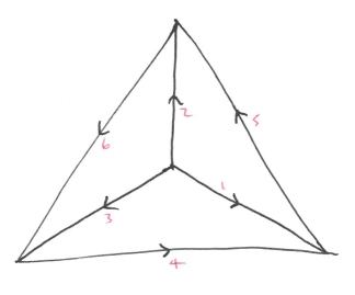
   Figure 2: Regular tetrahedron

2. Regular cube, having $12$ edges of length $\theta_{1}=70.529^{\circ}$.

   Applying the $C^{0}$ and $C^{1}$ conditions (10), and using that all edges have the same length, gives directly the relations

   $$f(6)=-A\cos(\theta),\quad f(7)=A\cos(\theta),\quad f(9)=A\cos(\theta),\quad f(10)=-A\cos(\theta),$$ (11)

   $$\quad f(5)=-A\cos(\theta),\quad f(4)=A\cos(\theta),$$ (12)

   where $A$ is the same constant. But then, applying (10) at vertex $(4,10,12)$ gives the relation $A\cos(\theta_{1})=-A\cos(\theta_{1})$, which can only hold if $A=0$. By symmetry we deduce that every $f(i)\equiv 0$.

   

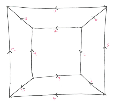
   Figure 3: Regular cube

3. Prism over regular pentagon, forming $15$ edges: “with the pentagonal arcs having length $\theta_{1}=41.810^{\circ}$ and the other arcs being of length $\theta_{2}=105.245^{\circ}$.”

   By the same reasoning as in the cube, taking into account the different lengths $\theta_{1}$, $\theta_{2}$, we have

   $$f(6)=A\cos(\theta),\quad f(5)=-A\cos(\theta),\quad f(14)=A\cos(\theta),\quad f(11)=-A\cos(\theta),$$ (13)

   for some constant $A$. We can therefore apply the $C^{1}$ condition at each end of $\ell(9)$, to see that

   $$f(9)=-A\sin(\theta_{1})\sin(\theta)-A(\cos(\theta_{1})+1)\cos(\theta).$$ (14)

   Apply both conditions at vertex $7,5,4$ to obtain

   $$f(7)=A\sin(\theta_{2})\sin(\theta)-A(\cos(\theta_{2})+\sin(\theta_{2})\frac{\cos(\theta_{1})}{\sin(\theta_{1})})\cos(\theta).$$ (15)

   These, together with $f(6)$, give three conditions on $f(8)$, and we obtain the relation

   $$A(4\sin\theta_{2}\cos\theta_{1}+2\sin\theta_{1}\cos\theta_{2}-\sin\theta_{2})=0.$$ (16)

   The term in the brackets is $-3.5$, to one decimal place. We deduce that $A=0$, and it’s straightforward to verify that $f(i)\equiv 0$ for every $i$.

   

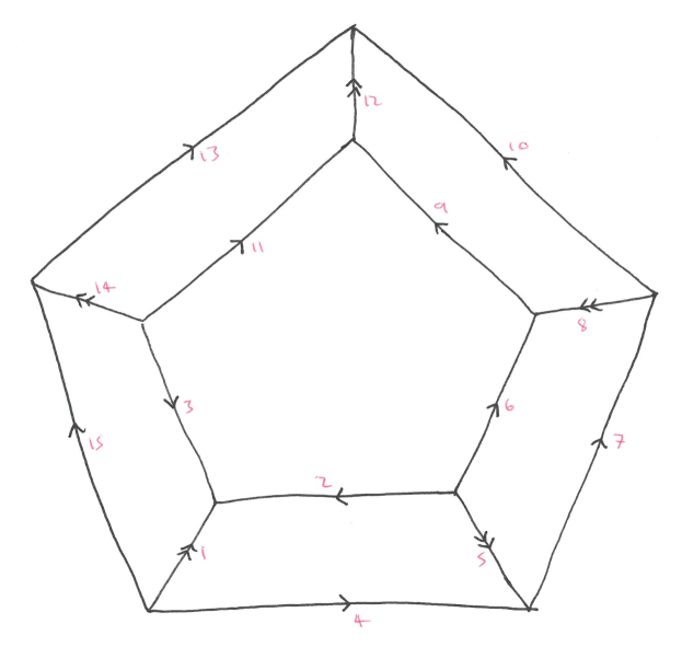
   Figure 4: Prism over regular pentagon

4. Prism over a regular triangle, forming $9$ edges: “the triangular arcs being of length $109.471^{\circ}$ and the other arcs of length $38.942^{\circ}$.”

   By same reasoning as the tetrahedron, we can apply the $C^{1}$ condition on each side of $\ell(7)$ to see $f(7)=0$. Apply both $C^{0}$- and $C^{1}$-condition at vertex $(2,6,7)$ to obtain $f(6)(0)=f(6)^{\prime}(0)=0$, and hence $f(6)=0$. Similarly, we have $f(8)=0$. We then deduce directly that $f(5)=f(9)=f(4)=0$.

   

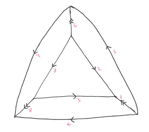
   Figure 5: Prism over regular triangle

5. Regular dodecahedron, having $30$ edges, each of length $\theta_{1}=41.810^{\circ}$.

   

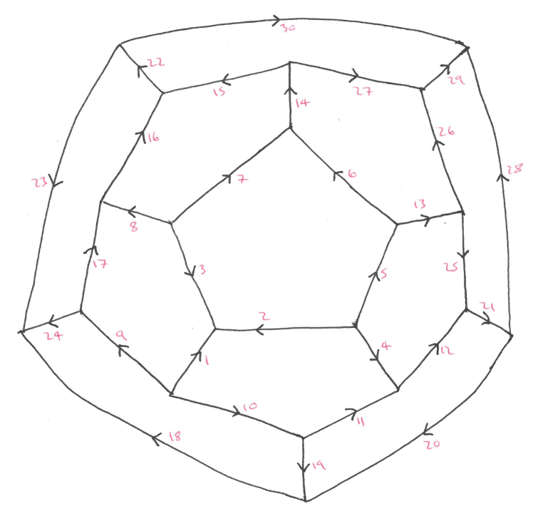
   Figure 6: Regular dodecahdron

   We have immediately the equations

   $$f(5)=A\cos\theta,\quad f(4)=-A\cos\theta,\quad f(10)=B\cos\theta,\quad f(9)=-B\cos\theta,$$ (17)

   $$\quad f(8)=G\cos\theta,\quad f(7)=-G\cos\theta,$$ (18)

   for some constants $A,B,G$. By symmetry it will suffice to show that $A=B=G=0$. We obtain, using the above and the compatibility conditions,

   $$f(11)=-B\sin\theta_{1}\sin\theta-(B\cos\theta_{1}+A)\cos\theta,$$ (19)

   $$f(17)=B\sin\theta_{1}\sin\theta+(G+B\cos\theta_{1})\cos\theta,$$ (20)

   $$f(6)=-A\sin\theta_{1}\sin\theta-(A\cos\theta_{1}+G)\cos\theta,$$ (21)

   $$f(13)=-A\sin\theta_{1}\sin\theta+(G+2A\cos\theta_{1})\cos\theta,$$ (22)

   $$f(12)=A\sin\theta_{1}\sin\theta-(2A\cos\theta_{1}+B)\cos\theta,$$ (23)

   $$f(24)=B\sin\theta_{1}\sin\theta-(2B\cos\theta_{1}+G)\cos\theta,$$ (24)

   $$f(19)=-B\sin\theta_{1}\sin\theta+(A+2B\cos\theta_{1})\cos\theta,$$ (25)

   $$f(25)=-(G+3A\cos\theta_{1})\sin\theta_{1}\sin\theta-(G\cos\theta_{1}+3A\cos^{2}\theta_{1}+3A\cos\theta_{1}+B)\cos\theta,$$ (26)

   and

   $$f(21)=(3A\sin\theta_{1}\cos\theta_{1}+B\sin\theta_{1})\sin\theta+(-G-2B\cos\theta_{1}-6A\cos^{2}\theta_{1}-3A\cos\theta_{1}+A)\cos\theta.$$ (27)

   And

   $$f(20) =\left[A(9\cos^{2}\theta_{1}+3\cos\theta_{1}\sin\theta_{1}-\sin\theta_{1})+3B\sin\theta_{1}\cos\theta_{1}+G\sin\theta_{1}\right]\sin\theta$$ (28)

   $$\quad\left[A(9\cos^{3}\theta_{1}+3\cos^{2}\theta_{1}-\cos\theta_{1}+1)+B(3\cos^{2}\theta_{1}+3\cos\theta_{1})+G\cos\theta_{1}\right]\cos\theta.$$ (29)

   From $19$ and $24$, we obtain

   $$f(18)=-(3B\sin\theta_{1}\cos\theta_{1}+A\sin\theta_{1})\sin\theta-(A\cos\theta_{1}+3B\cos^{2}\theta_{1}+3B\cos\theta_{1}+G)\cos\theta.$$ (30)

   But we have additionally $20$, which implies the relation:

   $$2G=A(-9\cos^{2}\theta_{1}-6\cos\theta_{1}+1)+B(-9\cos^{2}\theta_{1}-6\cos\theta_{1}+1).$$ (31)

   We work upwards. We have

   $$f(14)=G\sin\theta_{1}\sin\theta-(2G\cos\theta_{1}+A)\cos\theta,$$ (32)

   $$f(16)=-G\sin\theta_{1}\sin\theta+(B+2G\cos\theta_{1})\cos\theta,$$ (33)

   $$f(15)=(3G\cos\theta_{1}\sin\theta_{1}+A\sin\theta_{1})\sin\theta+(3G\cos^{2}\theta_{1}+3G\cos\theta_{1}+A\cos\theta_{1}+B)\cos\theta$$ (34)

   And

   $$f(26)=-(3A\sin\theta_{1}\cos\theta_{1}+G\sin\theta_{1})\sin\theta+(2G\cos\theta_{1}+B+6A\cos^{2}\theta_{1}+3A\cos\theta_{1}-A)\cos\theta$$ (35)

   We calculate $27$. Using $14$, $15$, we obtain

   $$f(27)=(3G\sin\theta_{1}\cos\theta_{1}+A\sin\theta_{1})\sin\theta+(G-6G\cos^{2}\theta_{1}-3G\cos\theta_{1}-2A\cos\theta_{1}-B)\cos\theta.$$ (36)

   Combining this with $26$ gives the relation:

   $$2B=A(-9\cos^{2}\theta_{1}-6\cos\theta_{1}+1)+G(-9\cos^{2}\theta_{1}-6\cos\theta_{1}+1).$$ (37)

   Let us proceed to the left. We have

   $$f(22)=-(3G\sin\theta_{1}\cos\theta_{1}+B\sin\theta_{1})\sin\theta+(6G\cos^{2}\theta_{1}+3G\cos\theta_{1}-G+A+2B\cos\theta_{1})\cos\theta.$$ (38)

   Using $22$ and $24$ we obtain

   $$f(23)=\left[G(-9\cos^{2}\theta_{1}\sin\theta_{1}-3\cos\theta_{1}\sin\theta_{1}+\sin\theta_{1})-A\sin\theta_{1}-3B\sin\theta_{1}\cos\theta_{1}\right]\sin\theta$$ (39)

   $$\quad+\left[G(-9\cos^{3}\theta_{1}-3\cos^{2}\theta_{1}+\cos\theta_{1}-1)-A\cos\theta_{1}-B(3\cos^{2}\theta_{1}+3\cos\theta_{1})\right]\cos\theta.$$ (40)

   But now using additionally $18$, we obtain the relation

   $$2A=G(-9\cos^{2}\theta_{1}-6\cos\theta_{1}+1)+B(-9\cos^{2}\theta_{1}-6\cos\theta_{1}+1).$$ (41)

   We thus have the three equations

   $$A=\alpha(B+G),\quad B=\alpha(A+G),\quad G=\alpha(A+B),$$ (42)

   where $\alpha=1.5$ (to one decimal place). One easily verifies the only solution to (42) is when $A=B=G=0$, and by symmetry we deduce that $f(i)=0$ for every $i$.

6. Two regular quadrilaterals and eight equal pentagons, forming $24$ edges: “each quadrilateral surrounded by four pentagons, and each pentagons surrounded by four pentagons and one quadrilateral, the quadrilateral arcs being of length $\theta_{2}=70.529^{\circ}$, the arcs adjacent to no quadrilateral vertex being of length $\theta_{3}=52.448^{\circ}$, and the remaining edges being of length $\theta_{1}=21.428^{\circ}$.”

   

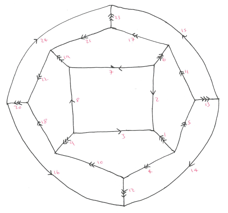
   Figure 7: Two regular quadrilaterals and eight equal pentagons

   We have directly that

   $$f(4)=-A\cos\theta,\quad f(5)=A\cos\theta,$$ (43)

   $$\quad f(6)=-B\cos\theta,\quad f(7)=B\cos\theta,\quad f(8)=B\cos\theta,\quad f(9)=-B\cos\theta,$$ (44)

   for some constants $A,B$. Using the compatability conditions at various vertices, we obtain

   $$f(10)=A\sin\theta_{3}\sin\theta+(A\cos\theta_{3}-B\frac{\sin\theta_{1}}{\sin\theta_{3}})\cos\theta$$ (45)

   $$f(11)=-A\sin\theta_{3}\sin\theta-(A\cos\theta_{3}+B\frac{\sin\theta_{1}}{\sin\theta_{3}})\cos\theta$$ (46)

   $$f(12)=A\sin\theta_{3}\sin\theta+(-2A\cos\theta_{3}+B\frac{\sin\theta_{1}}{\sin\theta_{3}})\cos\theta$$ (47)

   $$f(13)=-A\sin\theta_{3}\sin\theta+(2A\cos\theta_{3}+B\frac{\sin\theta_{1}}{\sin\theta_{3}})\cos\theta$$ (48)

   $$f(18)=B\sin\theta_{1}\sin\theta+(-B\cos\theta_{1}-B\sin\theta_{1}\frac{\cos\theta_{3}}{\sin\theta_{3}}+A)\cos\theta$$ (49)

   $$f(19)=-B\sin\theta_{2}\sin\theta+2B\cos\theta_{2}\cos\theta$$ (50)

   $$f(17)=B\sin\theta_{1}\sin\theta-(B\cos\theta_{1}+B\sin\theta_{1}\frac{\cos\theta_{3}}{\sin\theta_{3}}+A)\cos\theta$$ (51)

   And we have

   $$f(22)=\left[-B\sin\theta_{2}\cos\theta_{1}-2B\cos\theta_{2}\sin\theta_{1}\right]\sin\theta$$ (52)

   $$\quad+\left[B\frac{-\cos\theta_{1}\sin\theta_{2}\cos\theta_{3}-2\sin\theta_{1}\cos\theta_{2}\cos\theta_{3}-2\sin\theta_{1}\cos\theta_{3}}{\sin\theta_{3}}-B\cos\theta_{1}+A\right]\cos\theta.$$ (53)

   Using $17$ and $19$, we obtain

   $$f(21)=(2B\sin\theta_{1}\cos\theta_{3}+B\cos\theta_{1}\sin\theta_{3}+A\sin\theta_{3})\sin\theta$$ (54)

   $$\quad+\left[B\frac{2\sin\theta_{1}\cos^{2}\theta_{3}+\cos\theta_{1}\sin\theta_{2}+2\sin\theta_{1}\cos\theta_{2}}{\sin\theta_{3}}+B\cos\theta_{1}\cos\theta_{3}+A\cos\theta_{3}\right]\cos\theta$$ (55)

   But then we can use the $C^{0}$ condition with $22$ to get the relation

   $$0 =B\left[2\sin\theta_{1}\cos\theta_{3}\sin\theta_{3}+2\cos\theta_{1}+2\cos\theta_{1}\cos\theta_{2}-\sin\theta_{1}\sin\theta_{2}\right.$$ (56)

   $$\quad\left.+\frac{\cos\theta_{3}}{\sin\theta_{3}}(-2\sin^{3}\theta_{1}+2\cos\theta 0\sin\theta_{1}+4\sin\theta_{1}\cos\theta_{2})\right].$$ (57)

   Notice the terms involving $A$ cancel! One can readily calculate the term in the brackets is $=3.3$ (to one decimal place), and therefore we must have $B=0$. We deduce

   $$f(6)=f(7)=f(8)=f(9)=f(19)=0.$$ (58)

   We now calculate

   $$f(14)=A(-\sin\theta_{3}\cos\theta_{1}-2\cos\theta_{3}\sin\theta_{1})\sin\theta$$ (59)

   $$\quad+A(\sin\theta_{2})^{-1}\left[-\cos\theta_{1}\cos\theta_{2}\sin\theta_{3}-2\sin\theta_{1}\cos\theta_{2}\cos\theta_{3}-\cos\theta_{1}\sin\theta_{3}-2\cos\theta_{3}\cos\theta_{1}\right]\cos\theta.$$ (60)

   And

   $$f(20)=-A\sin\theta_{3}\sin\theta+2A\cos\theta_{3}\cos\theta.$$ (61)

   Since $B=0$ we see $f(20)$ has precisely the same form as $f(13)$, and so by using $20$ and $12$ we see that $f(16)$ correspondingly has the same expression as $f(14)$. Now we can additionally use the $C^{0}$ condition at vertex $(14,12,16)$ to get the condition

   $$A\left[-2\cos\theta_{1}\sin\theta_{3}-4\sin\theta_{1}\cos\theta_{3}-2\cos\theta_{1}\cos\theta_{2}\sin\theta_{3}-4\sin\theta_{1}\cos\theta_{2}\right.$$ (62)

   $$\quad\left.+\sin\theta_{1}\sin\theta_{2}\sin\theta_{3}-2\cos\theta_{1}\sin\theta_{2}\cos\theta_{3}\right]=0.$$ (63)

   The term in the brackets is $-3.8$ (to one decimal), and we deduce $A=0$ also. By symmetry we deduce $f(i)=0$ for all $i$.

7. Four equal quadrilaterals and four equal pentagons, forming $18$ edges: “each quadrilateral surrounded by three pentagons and one quadrilateral, and each pentagon by three quadrilaterals and two pentagons, and having the arcs held in common by two quadrilaterals (and the quadrilateral arcs opposite to them) being of length $\theta_{3}=83.802^{\circ}$ and the other quadrilateral arcs of length $\theta_{2}=58.257^{\circ}$ and all remaining edges of length $\theta_{1}=13.559^{\circ}$.”

   

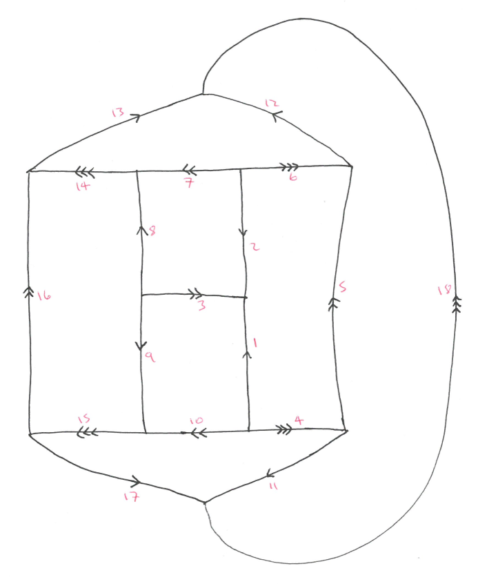
   Figure 8: Four equal quadrilaterals and four equal pentagons

   Let us calculate. We have directly

   $$f(4)=A\cos\theta,\quad f(10)=-A\cos\theta,\quad f(9)=-A\frac{\sin\theta_{3}}{\sin\theta_{2}}\cos\theta,\quad f(8)=A\frac{\sin\theta_{3}}{\sin\theta_{2}}\cos\theta,$$ (64)

   $$\quad f(7)=A\cos\theta,\quad f(6)=-A\cos\theta,$$ (65)

   for some constant $A$. We have

   $$f(5)=-A\sin\theta_{1}\sin\theta-(A\sin\theta_{1}\frac{\cos\theta_{3}}{\sin\theta_{3}}+A\frac{\sin\theta_{1}}{\sin\theta_{3}})\cos\theta$$ (66)

   $$f(14)=-A\sin\theta_{3}\sin\theta+(A\cos\theta_{3}+A\frac{\sin\theta_{3}}{\sin\theta_{2}}\cos\theta_{2})\cos\theta$$ (67)

   $$f(15)=A\sin\theta_{3}\sin\theta-(A\cos\theta_{3}+A\frac{\sin\theta_{3}}{\sin\theta_{2}}\cos\theta_{2})\cos\theta$$ (68)

   And

   $$f(16)=A(\cos\theta_{1}\sin\theta_{3}+\sin\theta_{1}\cos\theta_{3}+\frac{\sin\theta_{1}\cos\theta_{2}\sin\theta_{3}}{\sin\theta_{2}})(\sin\theta+\frac{\cos\theta_{3}+1}{\sin\theta_{3}}\cos\theta).$$ (69)

   We have

   $$f(17)=A\left[\cos\theta_{1}\sin\theta_{3}+\sin\theta_{1}\cos\theta_{3}+\frac{\sin\theta_{1}\cos\theta_{2}\sin\theta_{3}}{\sin\theta_{2}}\right]\sin\theta$$ (70)

   $$\quad+A\left[\sin\theta_{1}\sin\theta_{3}-\cos\theta_{1}\cos\theta_{3}-\frac{\cos\theta_{1}\cos\theta_{2}\sin\theta_{3}}{\sin\theta_{2}}\right.$$ (71)

   $$\quad\quad\left.-(\frac{\cos\theta_{3}+1}{\sin\theta_{3}})(\cos\theta_{1}\sin\theta_{3}+\sin\theta_{1}\cos\theta_{3}+\frac{\sin\theta_{1}\cos\theta_{2}\sin\theta_{3}}{\sin\theta_{2}})\right]\cos\theta.$$ (72)

   Now using $4$, $5$, we obtain

   $$f(11)=-A\sin\theta_{1}\sin\theta+A(\frac{\sin\theta_{1}}{\sin\theta_{3}}+\sin\theta_{1}\frac{\cos\theta_{3}}{\sin\theta_{3}}+\cos\theta_{1})\cos\theta.$$ (73)

   But we additionally have a condition with $17$, giving us the relation:

   $$A\left[2\sin\theta_{1}\cos\theta_{2}+2\sin\theta_{1}\cos\theta_{2}\cos\theta_{3}+2\frac{\sin\theta_{1}\sin\theta_{2}}{\sin\theta_{3}}+\frac{\sin\theta_{1}\sin\theta_{3}}{\sin\theta_{2}}-3\sin\theta_{1}\sin\theta_{2}\sin\theta_{3}\right.$$ (74)

   $$\quad\left.+2\frac{\sin\theta_{1}\sin\theta_{2}\cos\theta_{3}}{\sin\theta_{3}}+2\cos\theta_{1}\sin\theta_{2}+2\cos\theta_{1}\cos\theta_{2}\sin\theta_{3}+2\cos\theta_{1}\sin\theta_{2}\cos\theta_{3}\right]=0.$$ (75)

   Therefore we must have $A=0$. It follows directly that $f(i)=0$.

8. Three regular quadrilaterals and six equal pentagons, forming $21$ edges: “each quadrilateral surrounded by four pentagons and each pentagon by two quadrilaterals and three pentagons, with the quadrilateral edge being of length $\theta_{2}=70.529^{\circ}$, the pentagonal edge adjacent to just one quadrilateral vertex being of length $\theta_{3}=35.264^{\circ}$, and the remaining three edges of length $\theta_{1}=10.529^{\circ}$.”

   

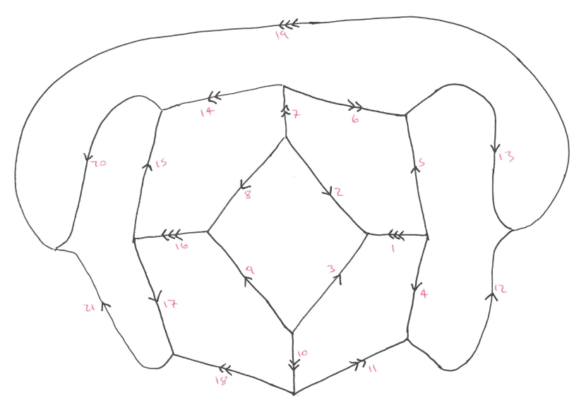
   Figure 9: Three regular quadrilaterals and six equal pentagons

   We have directly that

   $$f(7)=A\cos\theta,\quad f(8)=-A\cos\theta,\quad f(9)=-A\cos\theta,\quad f(10)=A\cos\theta$$ (76)

   $$\quad f(5)=B\cos\theta,\quad f(4)=-B\cos\theta,$$ (77)

   for some constants $A,B$. We obtain

   $$f(6)=-A\sin\theta_{3}\sin\theta+(-A\cos\theta_{3}+B\frac{\sin\theta_{2}}{\sin\theta_{3}})\cos\theta$$ (78)

   $$f(11)=-A\sin\theta_{3}\sin\theta-(A\cos\theta_{3}+B\frac{\sin\theta_{2}}{\sin\theta_{3}})\cos\theta$$ (79)

   $$f(12)=B\sin\theta_{2}\sin\theta-(B\sin\theta_{2}\frac{\cos\theta_{3}}{\sin\theta_{3}}+B\cos\theta_{2}+A)\cos\theta$$ (80)

   $$f(13)=-B\sin\theta_{2}\sin\theta+(B\sin\theta_{2}\frac{\cos\theta_{3}}{\sin\theta_{3}}+B\cos\theta_{2}-A)\cos\theta.$$ (81)

   But now we can use the $C^{1}$ condition at vertex $12,19,13$ to get the relation

   $$B\left[2\cos\theta_{2}\sin\theta_{3}+\sin\theta_{2}\cos\theta_{3}\right]=0,$$ (82)

   which necessitates that $B=0$.

   We proceed by calculating

   $$f(16)=A\sin\theta_{2}\sin\theta-2A\cos\theta_{2}\cos\theta$$ (83)

   $$f(14)=f(18)=-A\sin\theta_{3}\sin\theta+2A\cos\theta_{3}\cos\theta$$ (84)

   $$f(15)=f(17)=(A\cos\theta_{1}\sin\theta_{2}+2A\sin\theta_{1}\cos\theta_{2})\sin\theta$$ (85)

   $$\quad+A\left[\frac{\cos\theta_{1}\cos\theta_{2}\sin\theta_{2}+2\sin\theta_{1}\cos^{2}\theta_{2}+3\sin\theta_{3}\cos\theta_{3}}{\sin\theta_{2}}\right]\cos\theta.$$ (86)

   But now we can apply the $C^{0}$ condition at vertex $16,15,17$ to get

   $$A\left[6\cos\theta_{3}\sin\theta_{3}+5\sin\theta_{1}\cos^{2}\theta_{2}-\sin\theta_{1}\right]=0,$$ (87)

   which implies $A=0$. It then follows directly that $f(i)=0$ for all $i$.

This completes the proof of integrability when $k=1$. Suppose now $k\geq 2$. We can handle the projection $\pi_{\mathbb{R}^{3}\times\{0\}}\circ v$ in precisely the same manner as above. On the other hand, given any coordinate vector $e\in\{0\}\times\mathbb{R}^{k-1}$, let us define

$$f(i)(\theta)=e\cdot v(i)(\theta),$$ (88)

and observe $f(i)$ takes the same form (8). By Lemma LABEL:lem:vect-vs-scalar-cond the compatibility conditions are now

$$f(i_{1})(p)=f(i_{2})(p)=f(i_{3})(p),\quad\text{and}\quad\sum_{j=1}^{3}(n(i_{j})\cdot\hat{\ell}(i_{j}))f^{\prime}(i_{j})(p)=0,$$ (89)

whenever $\ell(i_{1}),\ell(i_{2}),\ell(i_{3})$ share a common vertex $p$. Since $f^{\prime\prime}+f=0$, we see that the functions $f^{\prime}(i)$ satisfy conditions (9), (10), and we can apply the proof above to deduce every $f^{\prime}(i)=0$. This implies $f=0$, and hence $\pi_{\{0\}\times\mathbb{R}^{k-1}}\circ v$ is zero also. ∎