Total Roto-Translational Variation

Abstract

We consider curvature depending variational models for image regularization, such as Euler’s elastica. These models are known to provide strong priors for the continuity of edges and hence have important applications in shape- and image processing. We consider a lifted convex representation of these models in the roto-translation space: In this space, curvature depending variational energies are represented by means of a convex functional defined on divergence free vector fields. The line energies are then easily extended to any scalar function. It yields a natural generalization of the total variation to the roto-translation space. As our main result, we show that the proposed convex representation is tight for characteristic functions of smooth shapes. We also discuss cases where this representation fails. For numerical solution, we propose a staggered grid discretization based on an averaged Raviart-Thomas finite elements approximation. This discretization is consistent, up to minor details, with the underlying continuous model. The resulting non-smooth convex optimization problem is solved using a first-order primal-dual algorithm. We illustrate the results of our numerical algorithm on various problems from shape- and image processing.
Keywords: Image processing, shape processing, image inpainting, curvature, Elastica, roto-translations, convex relaxation, total variation.
AMS MSC (2010): 53A04   49Q20   26A45   35J35   53A40   65K10

1 Introduction

It was observed at least since [58] that line energies such as Euler’s “Elastica” (here for a smooth curve $\gamma$):

$$\int_{\gamma}[1+]\;\kappa^{2}ds$$

could be natural regularizers for the completion of missing contours in images. This idea was based in particular on observations of G. Kanizsa [46, 47] about the way our perception can “invent” apparent contours. The model in [58] (see also [40, 39] for interesting attempts to solve it with phase-field methods) was variational in nature and since then, many attempts have been proposed to study and address the minimization of such line energies, both theoretically and numerically.

From the theoretical point of view, the lower-semicontinuity of these energies already is a challenge, which has been studied in many papers (in connexion to the applications to computer vision) since at least the 90s [12, 13, 16, 14, 17, 15, 30]. It is shown already in [12] that the boundary of many sets with cusps can be approximated by sets with smooth boundaries of bounded energy, showing that the relaxation of the Elastica for boundaries of sets is already far from trivial. The study of this lower semi-continuity of course enters the long history of the study of general curvature dependent energies of manifolds and in particular the Willmore energy [77].

Quite early, it has been suggested to lift the manifold in a larger space where a variable represents its direction or orientation, by means in particular (for co-dimension one manifolds) of the Gauss map $(x,\nu(x))$, $\nu(x)$ being the normal to the manifold at $x$ [5, 6]. Such approach allows to study very general curvature energies and has been successfully used for establishing lower-semicontinuity and existence results [6, 7, 32, 31], and in particular to lines energies such as ours in higher codimension [2, 1] or in dimension 2 [31]. We must mention also in this class an older approach based on “curvature varifolds” (which is very natural since varifolds are defined on the cross product of spatial and directional variables) which has allowed to show existence results since the 80s [45], see also [50].

Interestingly, it was understood much earlier [44] that (cats’) vision was functioning in a similar way (eg., using a sort of “Gauss map”), thanks to neurons sensitive to particular directions which were found to be stacked inside the visual cortex into ordered columns, making us sensitive to changes of orientations (and thus curvature intensity). These findings (which might explain some of Kanizsa’s experiments) inspired some mathematical models quite early [48], however they were formalized into a consistent geometric interpretation later on [59, 66, 65, 29, 57, 33]. The idea of these authors is to lift 2D curves in the “Roto-translation” space (which is the group of rotations and translations, however what is more important here is less its group structure than the associated sub-Riemanian metrics) which can be identified, for our purposes, with ${\Omega\times\mathbb{S}^{1}}$ where $\Omega\subset\mathbb{R}^{2}$ is the spatial domain where the image is defined and $\mathbb{S}^{1}$ parameterizes the local orientation.

The natural metric in that space prevents from moving spatially in a direction other than the local orientation, which makes it singular (hence “sub”-Riemanian). Diffusion and mean curvature flow in this particular metrics were successfully used as efficient methods for image “inpainting”, which is the task of filling in a gap in an image [41, 19, 61, 72]. Indeed, such diffusion naturally extends missing level sets into smooth curves, and even allows for crossing, since curves with different directions “live” in different locations in the Roto-translation space. This seems to improve in difficult situations (eg., crossings) upon more classical diffusion models for inpainting [27, 18] (or Weickert’s “EED” [75, 76, 67] which can propagate directional information quite smoothly accross inpainted regions).

In computer science, similar ideas were successfully implemented in discrete graphs (with nodes representing a spatial point and orientation) in order to minimize curvature-dependent contour energies [68, 37, 36, 70, 49, 69, 71, 38]. Our current work is closer to these approaches, although set up in the continuous setting, as we want to represent and solve variational models involving curvature terms, were the unknown are scalar (grey-level) functions. A continuous approach similar to these discrete ones proposes to compute minimal paths in the Roto-translational metric by solving the corresponding eikonal equations [55, 56, 28] (the goal being more here to find paths on an image than to complete boundaries). This is strongly connected to geometric control problems (such as parking a car), and these connections have led to the study many interesting metrics in these settings, with impressive applications to imaging problems such as the extraction of networks of vessels and fibers in 2D and 3D medical images via fast, globally optimal sub-Riemannian and sub-Finslerian geodesic tracking in the roto-translation group [11, 34].

As said, we wish to extend these variational methods to level sets representations. The family of problems we are interested in is introduced in a paper by Masnou and Morel [52] (see also [53]), which addresses the problem of image inpainting. Their initial idea is to minimize, in the inpainting domain $D$, an energy of the form

$$\int_{D}\left(1+\left|\textup{div}\,\frac{Du}{|Du|}\right|^{p}\right)|Du|$$

for some $p\geq 1$, where $u$ is a bounded variation function and appropriate boundary conditions are given. A theoretical study of this energy, which in general is not lower-semicontinuous (lsc), is found in [4], in particular it is shown that if $p>1$ (in dimension $2$), it is lsc on $C^{2}$ functions. Interestingly, also this study relies on a space/direction representation (and more precisely on varifolds). An interesting co-area formula for the relaxed envelope is also shown in [51].

There have been many attempts to numerically solve Masnou and Morel’s model, which is very difficult to tackle, being highly non convex. Most of the authors introduce auxiliary variables [9, 26, 10], for instance representing the orientation, which is already close to the idea of the Gauss map or Roto-translational representation. Recent techniques based on Augmented Lagrangian methods (for coupling the auxiliary variables) [74, 80, 78, 79, 43, 42, 8] have shown to be quite efficient, despite the lack of convexity and hence convergence guaranties.

What we propose here is to rather introduce a functional which may be sees as a convex relaxation of Masnou and Morel’s. The method we propose is based on two ingredients: A lifting in the Roto-translation space of curves which allows to write the Elastica energy (or any convex function of the curvature) as a convex function, as in classical Gauss map based approaches, and (formally) a decomposition of functions as sum of characteristic functions of sets with finite energy. This allows to define a convex functional which is defined on grey-level functions and penalises the curvature of the level lines. It is however easy to check that it is in general strictly below Masnou and Morel’s functional, in particular a function of finite energy needs not have its level sets regular (in practice, they could be intersections of regular sets, in addition to having possible cusps, for the same reasons as in [12]), see for example Figures 5 and 9(e). The only theoretical result which we can show is that $C^{2}$ curves are tightly represented by our convex relaxation.

There is a close relationship between our approach and the functionals in [22] (“TVX”) and [23], based on similar representations (but [22] omits to preserve the boundary of the lifted current). In fact, the functional we build is, as we show further on, a new expression of the previous convex relaxation of the Elastica energy (and variants) proposed in [23]. This stems from the identity of the corresponding dual problems. Although it boils down to the same energy, it is introduced in a much simpler way, as the primal expression in [23] requires to work in a space where the point, the tangent and the curvature are lifted as independent variables. As a consequence, we also can provide a simpler discretization, and the tightness of the relaxation for $C^{2}$ sets was unnoticed in [23]. Eventually, we should mention that part of what we propose here could be generalized to arbitrary dimension or co-dimension, following the techniques in [6]. However, computationally, our construction for 1D curves in the plane already needs to work in a 3D space, and more complex models seem at this moment intractable. Our future research will rather focus on improving the discretization and the optimization of the bidimensional case.

The paper is organised as follows: In Section 2 we describe the lifting and introduce our functional. We state our main result, which shows that characteristic functions of $C^{2}$ sets are well represented by our convex relaxation (Theorem 1). In the next Section 3 we show an approximation result with smooth functions, and compute a dual representation of the functional (which shows it is identical to [23]). Then, in Section 4, we describe how the functional is discretized and show a few experimental results. The last Section 5 is devoted to the proof if Theorem 1. Some technical tools are found in the Appendix, in particular, Appendix A shows, up to (hopefully minor) transformations, the consistency of our implementation in Section 4.

2 The functional

We consider $\Omega$ a bounded open domain in the plane, and $E\subset\Omega$ a set with $C^{2}$ (and to simplify, connected) boundary. Assume that this boundary $\partial E$ is given by a parameterized curve $\left(x_{1}(t),x_{2}(t)\right)$ with parameter $t\in[0,1]$. The (extrinsic) curvature $\kappa_{E}$ of $\partial E$ is classically defined as the ratio between the variation of the tangential angle $\theta$ and the variation of its arc length $s$, that is

$$\kappa_{E}=\frac{d\theta}{ds}=\frac{\frac{d\theta}{dt}}{\frac{ds}{dt}}\frac{\frac{d\theta}{dt}}{\sqrt{\left(\frac{dx_{1}}{dt}\right)^{2}+\left(\frac{dx_{2}}{dt}\right)^{2}}}\;.$$

The main idea of the lifting is now to consider a higher dimensional representation of the parametric curve in the 3D roto-translation (RT) space, which is obtained by adding the tangential angle $\theta$ as an additional dimension to $\Omega$. In this space, we now consider a parameterized 3D curve $\left(x_{1}(t),x_{2}(t),\theta(t)\right)$ which lifts the boundary $\partial E$ to the roto-translational space. Figure 1 shows an example where we lift the boundary of a disk (which is a circle) to the RT space. Observe that the lifted boundary is represented by a 3D helix.

Now, we define for all $t\in[0,1]$ the tangential vector $p(t)=(p^{x}(t),p^{\theta}(t))$ with

$$p^{x}(t)=\left(\frac{dx_{1}(t)}{dt},\frac{dx_{2}(t)}{dt}\right),\quad p^{\theta}(t)=\frac{d\theta(t)}{dt},\quad|p^{x}(t)|=\sqrt{\left(\frac{dx_{1}(t)}{dt}\right)^{2}+\left(\frac{dx_{2}(t)}{dt}\right)^{2}}.$$

The curvature is therefore given by

$$\kappa_{E}(t)=\frac{p^{\theta}(t)}{|p^{x}(t)|},$$

In this work we consider $f:\mathbb{R}\to[0,+\infty]$ a convex, lsc function and want to define a convex lsc extension (to grey-level valued functions) of energies of the type

$$E\mapsto\int_{\partial E}f(\kappa_{E})d\mathcal{H}^{1}$$

where $E\subset\Omega$ is a set with $C^{2}$ boundary, and $\kappa_{E}$ is the curvature of the set. Using our tangential vector $p(t)$, it is easy to see that the energy can be (formally) written as

$$\int_{\partial E}f(\kappa_{E})d\mathcal{H}^{1}=\int_{0}^{1}f(p^{\theta}/|p^{x}|)|p^{x}|dt=\int_{{\Omega\times\mathbb{S}^{1}}}f(\tau^{\theta}/|\tau^{x}|)|\tau^{x}|d\mathcal{H}^{1}{{\mathchoice{\>\hbox{\vrule width=0.2pt\vbox to7.0pt{\vfill\hrule width=7.0pt,height=0.2pt}}\>}{\>\hbox{\vrule width=0.2pt\vbox to7.0pt{\vfill\hrule width=7.0pt,height=0.2pt}}\>}{\,\hbox{\vrule width=0.2pt\vbox to5.0pt{\vfill\hrule width=5.0pt,height=0.2pt}}\,}{\,\hbox{\vrule width=0.2pt\vbox to3.35pt{\vfill\hrule width=3.35pt,height=0.2pt}}\,}}}\Gamma_{E}$$

where $\Gamma_{E}=(x,\theta)([0,1])$ is the lifted curve and $\tau(x,\theta)$ its normalized tangential vector, given by $\tau(x(t),\theta(t))=p(t)/|p(t)|$ for all $t\in[0,1]$. A precise definition of the energy will be given below.

Figure 1: The gray line is the lifting of the boundary $\partial E$ of the disk $E$ to the roto-translational space ${\Omega\times\mathbb{S}^{1}}$.

Let us briefly discuss three instances of energies that will typically appear in applications. In all cases $\alpha>0$ will be a tuning parameter that can be used to balance the influence of the curvature term with respect to the length.

1. $f_{1}(t)=1+\alpha|t|$. This energy penalizes the arclength plus the absolute curvature, hence we might expect that this type of energy will allow also for corners. This type of energy has been studied with a different approach in [22]. The energy is given by:

   $$\int_{{\Omega\times\mathbb{S}^{1}}}f_{1}(\tau^{\theta}/|\tau^{x}|)|\tau^{x}|d\mathcal{H}^{1}{{\mathchoice{\>\hbox{\vrule width=0.2pt\vbox to7.0pt{\vfill\hrule width=7.0pt,height=0.2pt}}\>}{\>\hbox{\vrule width=0.2pt\vbox to7.0pt{\vfill\hrule width=7.0pt,height=0.2pt}}\>}{\,\hbox{\vrule width=0.2pt\vbox to5.0pt{\vfill\hrule width=5.0pt,height=0.2pt}}\,}{\,\hbox{\vrule width=0.2pt\vbox to3.35pt{\vfill\hrule width=3.35pt,height=0.2pt}}\,}}}\Gamma_{E}=\int_{{\Omega\times\mathbb{S}^{1}}}|\tau^{x}|+\alpha|\tau^{\theta}|d\mathcal{H}^{1}{{\mathchoice{\>\hbox{\vrule width=0.2pt\vbox to7.0pt{\vfill\hrule width=7.0pt,height=0.2pt}}\>}{\>\hbox{\vrule width=0.2pt\vbox to7.0pt{\vfill\hrule width=7.0pt,height=0.2pt}}\>}{\,\hbox{\vrule width=0.2pt\vbox to5.0pt{\vfill\hrule width=5.0pt,height=0.2pt}}\,}{\,\hbox{\vrule width=0.2pt\vbox to3.35pt{\vfill\hrule width=3.35pt,height=0.2pt}}\,}}}\Gamma_{E}.$$

2. $f_{2}(t)=\sqrt{1+\alpha^{2}|t|^{2}}$. This energy penalizes the arclength of the lifted curve in the RT space which, in some sense, corresponds to the “Total Roto-translational Variation”. It yields the energy:

   $$\int_{{\Omega\times\mathbb{S}^{1}}}f_{2}(\tau^{\theta}/|\tau^{x}|)|\tau^{x}|d\mathcal{H}^{1}{{\mathchoice{\>\hbox{\vrule width=0.2pt\vbox to7.0pt{\vfill\hrule width=7.0pt,height=0.2pt}}\>}{\>\hbox{\vrule width=0.2pt\vbox to7.0pt{\vfill\hrule width=7.0pt,height=0.2pt}}\>}{\,\hbox{\vrule width=0.2pt\vbox to5.0pt{\vfill\hrule width=5.0pt,height=0.2pt}}\,}{\,\hbox{\vrule width=0.2pt\vbox to3.35pt{\vfill\hrule width=3.35pt,height=0.2pt}}\,}}}\Gamma_{E}=\int_{{\Omega\times\mathbb{S}^{1}}}\sqrt{|\tau^{x}|^{2}+\alpha^{2}|\tau^{\theta}|^{2}}d\mathcal{H}^{1}{{\mathchoice{\>\hbox{\vrule width=0.2pt\vbox to7.0pt{\vfill\hrule width=7.0pt,height=0.2pt}}\>}{\>\hbox{\vrule width=0.2pt\vbox to7.0pt{\vfill\hrule width=7.0pt,height=0.2pt}}\>}{\,\hbox{\vrule width=0.2pt\vbox to5.0pt{\vfill\hrule width=5.0pt,height=0.2pt}}\,}{\,\hbox{\vrule width=0.2pt\vbox to3.35pt{\vfill\hrule width=3.35pt,height=0.2pt}}\,}}}\Gamma_{E}$$

   which is nothing but the length of the lifted curve $\Gamma_{E}$ in a Riemanian metric. This functional was considered for perceptional completion problems probably first in [65]. It coincides with sub-Riemannian [65, 33, 20, 11] and more precisely the sub-Finslerian models in [34] (with the constraint of positive direction on the velocity).

3. $f_{3}(t)=1+\alpha^{2}|t|^{2}$. This is the classical Eulers’s Elastica energy studied for example in [58, 12, 53, 68, 23] and many other works already mentioned in our introduction.

   $$\int_{{\Omega\times\mathbb{S}^{1}}}f_{3}(\tau^{\theta}/|\tau^{x}|)|\tau^{x}|d\mathcal{H}^{1}{{\mathchoice{\>\hbox{\vrule width=0.2pt\vbox to7.0pt{\vfill\hrule width=7.0pt,height=0.2pt}}\>}{\>\hbox{\vrule width=0.2pt\vbox to7.0pt{\vfill\hrule width=7.0pt,height=0.2pt}}\>}{\,\hbox{\vrule width=0.2pt\vbox to5.0pt{\vfill\hrule width=5.0pt,height=0.2pt}}\,}{\,\hbox{\vrule width=0.2pt\vbox to3.35pt{\vfill\hrule width=3.35pt,height=0.2pt}}\,}}}\Gamma_{E}=\int_{{\Omega\times\mathbb{S}^{1}}}|\tau^{x}|+\alpha^{2}\frac{|\tau^{\theta}|^{2}}{|\tau^{x}|}d\mathcal{H}^{1}{{\mathchoice{\>\hbox{\vrule width=0.2pt\vbox to7.0pt{\vfill\hrule width=7.0pt,height=0.2pt}}\>}{\>\hbox{\vrule width=0.2pt\vbox to7.0pt{\vfill\hrule width=7.0pt,height=0.2pt}}\>}{\,\hbox{\vrule width=0.2pt\vbox to5.0pt{\vfill\hrule width=5.0pt,height=0.2pt}}\,}{\,\hbox{\vrule width=0.2pt\vbox to3.35pt{\vfill\hrule width=3.35pt,height=0.2pt}}\,}}}\Gamma_{E}.$$

   Observe that the second term in the energy is a “quadratic over linear” function which is still convex, provided $\tau^{x}$ is constrained in a half space or a half line (which of course will depend on the $\theta$ variable).

In all these examples, we find that the energy which we are interested in ends up represented possibly as a convex function of the measure $\sigma=\tau\mathcal{H}^{1}{{\mathchoice{\>\hbox{\vrule width=0.2pt\vbox to7.0pt{\vfill\hrule width=7.0pt,height=0.2pt}}\>}{\>\hbox{\vrule width=0.2pt\vbox to7.0pt{\vfill\hrule width=7.0pt,height=0.2pt}}\>}{\,\hbox{\vrule width=0.2pt\vbox to5.0pt{\vfill\hrule width=5.0pt,height=0.2pt}}\,}{\,\hbox{\vrule width=0.2pt\vbox to3.35pt{\vfill\hrule width=3.35pt,height=0.2pt}}\,}}}\Gamma_{E}$. Moreover, this $\sigma$ is not an arbitrary measure. In particular, it satisfies two important constraints: first, by construction, it is a circulation and has zero divergence in ${\Omega\times\mathbb{S}^{1}}$ (it can have source terms on $\partial{\Omega\times\mathbb{S}^{1}}$): indeed, given any smooth function $\psi$, $\int\nabla\psi\cdot\sigma=\int_{\Gamma_{E}}\partial_{\tau}\psi d\mathcal{H}^{1}$ vanishes if $\Gamma_{E}$ is a closed curve, or if it ends on the boundary and $\psi$ has compact support. Second, its marginals in ${\Omega\times\mathbb{S}^{1}}$, which we can formally denote $\int_{S^{1}}\sigma$ (and which are also divergence free), coincide with a $90^{\circ}$-rotation of the measure $D\chi_{E}$. We will show now how to generalize this construction to arbitrary sets or functions (with bounded variation).

In the whole paper, we assume that there exists $\gamma>0$ such that

$$f(t)\geq\gamma\sqrt{1+t^{2}},\quad\forall\ t\in\mathbb{R}.$$ (1)

We also introduce the recession function

$$f^{\infty}(t)=\lim_{s\to+\infty}\frac{1}{s}f(st)$$

which is a convex, one-homogeneous function possibly infinite on $(-\infty,0)$ or/and $(0,+\infty)$. It is easy to check that it is the support function of $\textup{dom}\,f^{*}$, the domain of the convex conjugate $f^{*}$ of $f$:

$$f^{\infty}(t)=\sup_{y\in\textup{dom}\,f^{*}}ty.$$ (2)

Indeed, for $y\in\textup{dom}\,f^{*}$, $s>0$,

$$ty=\frac{1}{s}(st)y\leq\frac{1}{s}f(st)+\frac{1}{s}f^{*}(y)\stackrel{{\scriptstyle s\to\infty}}{{\longrightarrow}}f^{\infty}(t)$$

as $s\to\infty$; on the other hand, as $f^{*}\geq-\gamma$ thanks to (1), for $s>0$ one has

$$\frac{1}{s}f(st)=\sup_{y\in\textup{dom}\,f^{*}}ty-\frac{1}{s}f^{*}(y)\leq\sup_{y\in\textup{dom}\,f^{*}}ty+\frac{\gamma}{s}$$

showing that $f^{\infty}(t)\leq\sup_{y\in\textup{dom}\,f^{*}}ty$.

We let then, for $p=(p^{x},p^{\theta})\in\mathbb{R}^{3}$ with $p^{x}\neq 0$,

$$h(\theta,p)=\begin{cases}|p^{x}|f(p^{\theta}/|p^{x}|)&\textup{ if }p^{x}\in\mathbb{R}_{+}\underline{\theta},p^{x}\neq 0,\\ f^{\infty}(p^{\theta})&\textup{ if }p^{x}=0,\\ +\infty&\textup{ else.}\end{cases}$$ (3)

Here, $\underline{\theta}$ denotes the unit planar vector $(\cos\theta,\sin\theta)^{T}$ (by a slight abuse of notation, we will also denote in this way the vector $(\cos\theta,\sin\theta,0)^{T}\in\mathbb{R}^{3}$). It is then classical [64, § 13] and easily follows from (2) that one has

$$h(\theta,p)=\sup\left\{\xi\cdot p:\xi^{x}\cdot\underline{\theta}\leq-f^{*}(\xi^{\theta})\right\},$$ (4)

that is, the one-homogeneous function $h$ is the support function of the convex set in the right-hand side of (4). Indeed, first of all, the sup in (4) is $\infty$ if $p^{x}$ is not $\lambda\underline{\theta}$, $\lambda\geq 0$. While if it is of this form, then (taking the suprema over the $\xi$’s which satisfy $\xi^{x}\cdot\underline{\theta}\leq-f^{*}(\xi^{\theta})$)

$$\sup_{\xi\,:\,\xi^{x}\cdot\underline{\theta}\leq-f^{*}(\xi^{\theta})}\xi^{x}\cdot\underline{\theta}\lambda+\xi^{\theta}p^{\theta}=\sup_{\xi^{\theta}}\xi^{\theta}p^{\theta}-\lambda f^{*}(\xi^{\theta})=\begin{cases}\lambda f(p^{\theta}/\lambda)&\textup{ if }\lambda>0\\ f^{\infty}(p^{\theta})&\textup{ else.}\end{cases}$$

Observe that (1) yields that for all $p\in\mathbb{R}^{3}$,

$$h(\theta,p)\geq\gamma|p|$$ (5)

We now introduce the functional

$$F(u)=\inf\left\{\int_{{\Omega\times\mathbb{S}^{1}}}h(\theta,\sigma)dxd\theta\,:\,\textup{div}\,\sigma=0,\int_{\mathbb{S}^{1}}\sigma^{x}d\theta=Du^{\perp}\right\}.$$ (6)

Here $x^{\perp}=(x_{2},-x_{1})$ is a $90^{\circ}$ rotation in the plane. The last condition is understood as follows: for all $\varphi\in C_{c}^{1}(\Omega;\mathbb{R}^{2})\subset C_{c}^{1}({\Omega\times\mathbb{S}^{1}};\mathbb{R}^{2})$, one has

$$\int_{{\Omega\times\mathbb{S}^{1}}}\varphi^{\perp}\cdot\sigma^{x}=\int_{\Omega}\varphi\cdot Du=-\int_{\Omega}u\textup{div}\,\varphi dx.$$ (7)

In particular in general the fields $\sigma$ appearing in (6) are free-divergence bounded Radon measures in ${\Omega\times\mathbb{S}^{1}}$ with values in $\mathbb{R}^{3}$ (we denote $\mathcal{M}^{1}({\Omega\times\mathbb{S}^{1}};\mathbb{R}^{3})$ the space of such measures) and the proper way to write the integral is rather

$$\int_{{\Omega\times\mathbb{S}^{1}}}h(\theta,\sigma)=\int_{{\Omega\times\mathbb{S}^{1}}}h\left(\theta,\frac{\sigma}{|\sigma|}\right)d|\sigma|$$

where $\sigma/|\sigma|$ is the Radon-Besicovitch derivative of $\sigma$ w.r. its total variation $|\sigma|$. Notice that for any $u$ and any admissible $\sigma$, thanks to (5),

$$F(u)\geq\int_{{\Omega\times\mathbb{S}^{1}}}h(\theta,\sigma)\geq\gamma\int_{{\Omega\times\mathbb{S}^{1}}}|\sigma|\geq\gamma\int_{\Omega}|Du|$$

because of (7), taking the supremum with respect to the test function $\varphi$ with $|\varphi(x)|\leq 1$ everywhere. This shows that $F(u)$ bounds the $BV$ seminorm.

We denote by $K(\theta)$ the closed convex set of $\mathbb{R}^{3}$ whose support function is $h(\theta,\cdot)$, as already seen it is given by

$$K(\theta)=\left\{\xi\in\mathbb{R}^{3}:\xi^{x}\cdot\underline{\theta}\leq-f^{*}(\xi^{\theta})\right\}.$$

Remark that (1) implies that $f^{*}(s)\leq-\sqrt{\gamma^{2}-s^{2}}$ for $|s|\leq\gamma$, implying in particular that $0$ is in the interior of $K(\theta)$.

We then let (following for instance [21, 63])

$$K=\left\{\varphi\in C_{c}^{0}({\Omega\times\mathbb{S}^{1}};\mathbb{R}^{3}):\varphi(x,\theta)\in K(\theta)\;\forall(x,\theta)\in{\Omega\times\mathbb{S}^{1}}\right\}.$$

Then, we claim that for any measure $\sigma\in\mathcal{M}^{1}({\Omega\times\mathbb{S}^{1}};\mathbb{R}^{3})$

$$\int_{{\Omega\times\mathbb{S}^{1}}}h(\theta,\sigma)=\sup_{\varphi\in K}\int_{{\Omega\times\mathbb{S}^{1}}}\varphi\cdot\sigma,$$ (8)

showing in particular that this integral is a lower-semicontinuous function of $\sigma$ (for the weak-$*$ convergence). To prove this claim (which is standard), first observe that if $\varphi\in K$, then for all $\psi^{-}\in C_{c}^{0}({\Omega\times\mathbb{S}^{1}};\mathbb{R}_{+})$ and $\psi\in C_{c}^{0}({\Omega\times\mathbb{S}^{1}})$, also $\varphi-\psi^{-}\underline{\theta}+\psi\underline{\theta}^{\perp}\in K$. One deduces easily that the supremum in (8) is infinite if one of the measures $(\underline{\theta}\cdot\sigma^{x})^{-}$ or $\underline{\theta}^{\perp}\cdot\sigma^{x}$ does not vanish. If both vanish, it means that $\sigma=(\lambda\theta,\sigma^{\theta})$ for some nonnegative measure $\lambda$. Hence the supremum becomes

$$\sup_{\varphi\in K}\int_{{\Omega\times\mathbb{S}^{1}}}(\varphi^{x}\cdot\theta)\lambda+\varphi^{\theta}\sigma^{\theta}=\sup_{\psi+f^{*}(\varphi^{\theta})\leq 0}\int_{{\Omega\times\mathbb{S}^{1}}}\psi\lambda+\varphi^{\theta}\sigma^{\theta}=\sup_{\varphi^{\theta}}\int_{{\Omega\times\mathbb{S}^{1}}}\varphi^{\theta}\sigma^{\theta}-f^{*}(\varphi^{\theta})\lambda,$$

and (8) is then deduced in a standard way (with a Besicovitch covering of ${\Omega\times\mathbb{S}^{1}}$ with respect to the measure $|\sigma|$ by balls where $\lambda,\sigma^{\theta}$ are “almost constant”, and choosing then for $\varphi$ the “right function” in each ball of the covering—the fact that zero is in the interior of $K$, which allows to multiply functions in $K$ by a cut-off, is important here).

We can deduce that also $F$ is lower semicontinuous: consider a sequence $(u_{n})$ with $F(u_{n})\leq c<\infty$. Then $u_{n}$ is bounded in $BV$ and converges (up to a constant and a subsequence) to some $u$ in $L^{1}(\Omega)$.

If $\sigma_{n}$ reaches the value of $F(u_{n})$ up to $1/n$, one has that

$$\int_{{\Omega\times\mathbb{S}^{1}}}|\sigma_{n}|\leq c<\infty$$

so that $\sigma_{n}\stackrel{{\scriptstyle*}}{{\rightharpoonup}}\sigma$ (up to a subsequence), as measures, and obviously $\textup{div}\,\sigma=0$. Clearly, also (7) passes to the limit. Hence, by lower semicontinuity,

$$F(u)\leq\int_{{\Omega\times\mathbb{S}^{1}}}h(\theta,\sigma)\leq\liminf_{n}\int_{{\Omega\times\mathbb{S}^{1}}}h(\theta,\sigma_{n})=\liminf_{n}F(u_{n}).$$

This shows that $F$ defines a convex, lower semicontinuous functional on $BV(\Omega)$. Our main theoretical result is the following theorem, which shows that if the argument $u$ is the characteristic function of a smooth enough set, then $F(u)$ coincides, as expected, with a curvature-dependent energy of the boundary of the set $\{u=1\}$. The proof of this result is postponed to Section 5.

Theorem 1.

Let $E\subset\Omega$ be a set with $C^{2}$ boundary. Then

$$F(\chi_{E})=\int_{\partial E\cap\Omega}f(\kappa_{E}(x))d\mathcal{H}^{1}(x).$$ (9)

Remark 2.1.

One could hope that $F$ coincides with the lower semicontinuous envelope of its restriction to $C^{2}$ sets, with respect to the $L^{1}$ convergence. However, simple examples show that it is not the case. Many examples where it fails are found in [23]. In general, we expect the relaxation $F$ to be strictly below the relaxations found in the literature since [12], based on the ($L^{1}$) approximation of sets with smooths sets. In particular, in the case of [12, Fig. 4.2], our relaxation will certainly be below twice the energy reached by the pattern in [12, Fig. 1.2], while the energy reached in [12, Fig. 4.2] is strictly larger.

Remark 2.2.

If $f$ has growth one and is even, one expects that the same result holds for piecewise $C^{2}$ sets.

Remark 2.3.

We believe that the proof below could be extended to show that if $u\in BV(\Omega)$ is a function with $C^{2}$ level sets, and such that there exists a continuous function $\kappa(x)$ which coincides with the curvature of $\partial\{u>s\}$ for all level $s\in\mathbb{R}$, then one should have

$$F(u)=\int_{\mathbb{R}}\int_{\partial\{u>s\}}f(\kappa_{\partial\{u>s\}}(x))d\mathcal{H}^{1}(x)=\int_{\Omega}f(\kappa(x))d|Du|(x).$$ (10)

Hence in that case our functional would coincide with Masnou and Morel’s [53]. A typical example of a function $u$ for which such a function $\kappa(x)$ exists is (in a convex domain $\Omega$, see [54]) a solution of the so-called “Rudin-Osher-Fatemi” functional

$$\min_{u}\int_{\Omega}|Du|+\frac{\lambda}{2}\int_{\Omega}(u(x)-f(x))^{2}dx$$ (11)

for some $\lambda>0$, in case $f$ is continuous. Then, also $u$ is continuous and $\kappa(x)$ is given by $\lambda(u-f)$. In that case, in addition, $\kappa(x)$ is also the curvature of the level sets of $u^{\prime}=h(u)$ for any nondecreasing function $h$ such that $h(u)$ is still in $BV(\Omega)$.

3 Some properties of the functional

3.1 Approximation by smooth functions

Proposition 3.1.

Assume $\Omega$ is a bounded convex set. Then for any $u\in L^{1}(\Omega)$ with $F(u)<\infty$, there exists $(u_{n})_{n}$ a sequence of functions with $u_{n}\in C^{\infty}(\overline{\Omega})$, which converge to $u$ in $L^{1}(\Omega)$, and such that

$$\lim_{n\to\infty}F(u_{n})=F(u).$$

Remark 3.2.

We believe that, upon replacing $C^{\infty}(\overline{\Omega})$ with $C^{\infty}(\Omega)$, the result should be true in any domain.

Proof.

We assume, without loss of generality, that $0$ is in the interior of $\Omega$. It follows that for any $t<1$, $t\Omega\subset\subset\Omega$.

Consider $\rho$ a rotationally symmetric mollifier in $\mathbb{R}^{2}$ ($\rho\in C_{c}^{\infty}(B_{1}^{2};\mathbb{R}_{+})$, $\int\rho=1$, and we let $\rho_{\varepsilon}=(1/\varepsilon^{2})\rho(x/\varepsilon)$, where here $B_{1}^{d}$ is the unit $d$-dimensional ball). For $\varepsilon>0$, we consider the largest $t_{\varepsilon}<1$ such that $\{x\in\Omega:\textup{dist}\,(x,\partial\Omega)>\varepsilon\}\supseteq t_{\varepsilon}\Omega$. We then define $\sigma_{\varepsilon}$ as the measure on ${\Omega\times\mathbb{S}^{1}}$ given by

$$\int_{{\Omega\times\mathbb{S}^{1}}}\psi\cdot\sigma_{\varepsilon}=\int_{{\Omega\times\mathbb{S}^{1}}}\psi*\rho_{\varepsilon}(t_{\varepsilon}x,\theta)d\sigma(x),$$

where the convolution is only in the $x$-variable:

$$\psi*\rho_{\varepsilon}(x,\theta)=\int_{B_{1}^{2}}\psi(x-\varepsilon z,\theta)\rho(z)dz$$

and is well defined for $x\in t_{\varepsilon}\Omega$. It is clear that $\sigma_{\varepsilon}$ still has free divergence, moreover, if $\varphi\in C_{c}(\Omega;\mathbb{R}^{2})$,

$$\int_{{\Omega\times\mathbb{S}^{1}}}\varphi^{\perp}\cdot\sigma_{\varepsilon}^{x}=\int_{{\Omega\times\mathbb{S}^{1}}}\rho_{\varepsilon}*\varphi^{\perp}(t_{\varepsilon}x)\cdot\sigma_{\varepsilon}^{x}(x)=\int_{\Omega}\rho_{\varepsilon}*\varphi(t_{\varepsilon}x)\cdot Du\\ =-\int_{\Omega}\int_{B_{1}^{2}}t_{\varepsilon}u(x)\rho(z)\textup{div}\,\varphi(t_{\varepsilon}x-\varepsilon z)dzdx\\ =-\frac{1}{t_{\varepsilon}}\int_{\Omega}\int_{B_{1}^{2}}u((y+\varepsilon z)/t_{\varepsilon})\rho(z)\textup{div}\,\varphi(y)dzdy=-\frac{1}{t_{\varepsilon}}\int_{\Omega}(\rho_{\varepsilon/t_{\varepsilon}}*u)(y/t_{\varepsilon})\textup{div}\,\varphi(y)dy.$$

Hence, $\sigma_{\varepsilon}$ is admissible for the function $u_{\varepsilon}:y\mapsto\rho_{\varepsilon/t_{\varepsilon}}*u(y/t_{\varepsilon})/t_{\varepsilon}$, which clearly goes to $u$ in $L^{1}(\Omega)$ (or $BV(\Omega)$ weakly-$*$) as $\varepsilon\to 0$. Moreover, $u_{\varepsilon}\in C^{\infty}(\Omega)$ for all $\varepsilon>0$. Eventually, one has that for any $\varphi\in K$,

$$\int_{{\Omega\times\mathbb{S}^{1}}}\varphi\cdot\sigma_{\varepsilon}=\int_{{\Omega\times\mathbb{S}^{1}}}\varphi*\rho_{\varepsilon}(t_{\varepsilon}x,\theta)\cdot\sigma\leq\int_{{\Omega\times\mathbb{S}^{1}}}h(\theta,\sigma)=F(u)$$

by observing that since the convolution is only in the $x$ variable, $\varphi*\rho_{\varepsilon}(t_{\varepsilon}x,\theta)\in K(\theta)$ for all $(x,\theta)$ when $\varphi\in K$. Thanks to (8), it follows that

$$\int_{{\Omega\times\mathbb{S}^{1}}}h(\theta,\sigma_{\varepsilon})\leq F(u).$$

Hence $F(u_{\varepsilon})\leq F(u)$, and the proposition is proved. ∎

3.2 Dual representation

We can show the following representation for $F$, which in particular establishes that $F$ coincides exactly with the (more complicated) relaxation $R^{**}_{\textup{el}}$ defined in [23].

Proposition 3.3.

Assume $\partial\Omega$ is connected. Then the functional (6) can also be represented in the following form

$$F(u)=\sup\Bigg{\{}\int_{\Omega}\psi\cdot Du^{\perp}\,:\,\psi\in C^{0}_{c}(\Omega;\mathbb{R}^{2}),\\ \exists\,\varphi\in C_{c}^{1}({\Omega\times\mathbb{S}^{1}}),\underline{\theta}\cdot\left(\nabla_{x}\varphi+\psi\right)+f^{*}(\partial_{\theta}\varphi)\leq 0\Bigg{\}}.$$ (12)

If $\partial\Omega$ is not connected, then same formula holds, however the functions $\varphi$ should be in $C^{1}({\Omega\times\mathbb{S}^{1}})$, with $\nabla\varphi\in C_{c}^{0}({\Omega\times\mathbb{S}^{1}})$.

Corollary 3.4.

The functional $F(u)$ coincides with the relaxation of the Elastica energy $R^{**}_{\textup{el}}(u)$ defined in [23].

Indeed, formula (12) is the same as (35) in [23, Theorem 13]. The primal formulation (6) we introduce here is quite simpler as the original formulation in [23], though, as the “$\kappa$” variable is implicit in our formulation (it comes naturally as the derivative of the orientation) and does not need to be lifted.

Proof of Prop. 3.3.

We use the standard perturbation approach to duality [35], in the duality $(C_{0}^{0}({\Omega\times\mathbb{S}^{1}};\mathbb{R}^{3}),\mathcal{M}^{1}({\Omega\times\mathbb{S}^{1}};\mathbb{R}^{3}))$, where $C_{0}^{0}$ denotes the $L^{\infty}$-closure of the functions with compact support (hence, the functions which vanish on the boundary) and $\mathcal{M}^{1}$ the totally bounded vector-valued Radon measures. Defining, for $p\in\mathcal{M}^{1}({\Omega\times\mathbb{S}^{1}};\mathbb{R}^{3})$, the function

$$G(p)=\inf\left\{\int_{{\Omega\times\mathbb{S}^{1}}}h(\theta,\sigma+p)\,:\,\textup{div}\,\sigma=0,\int_{\mathbb{S}^{1}}\sigma^{x}=Du^{\perp}\right\}$$ (13)

so that $F(u)=G(0)$, we observe that $G$ is lower semicontinuous. Indeed if $p_{n}\stackrel{{\scriptstyle*}}{{\rightharpoonup}}p$ and $\sigma_{n}$ is a minimizer in the definition (13) of $G(p_{n})$, as before thanks to (5), $\sigma_{n}+p_{n}$ is bounded and up to a subsequence, converges to a measure $\sigma+p$ where $\sigma$ is admissible in (13). It follows that

$$G(p)\leq\int_{{\Omega\times\mathbb{S}^{1}}}h(\theta,\sigma+p)\leq\liminf_{n}\int_{{\Omega\times\mathbb{S}^{1}}}h(\theta,\sigma_{n}+p_{n})=\liminf_{n}G(p_{n}).$$

In particular, we deduce that $G=G^{**}$ so that

$$F(u)=G(0)=\sup_{\eta\in C_{0}^{0}({\Omega\times\mathbb{S}^{1}};\mathbb{R}^{3})}-G^{*}(\eta).$$

It remains to compute $G^{*}(\eta)$, to show that (12) follows:

$$G^{*}(\eta)=\sup_{p,\sigma}\int_{{\Omega\times\mathbb{S}^{1}}}\eta\cdot p-h(\theta,\sigma+p)=\sup_{\sigma}-\int_{{\Omega\times\mathbb{S}^{1}}}\eta\cdot\sigma+\sup_{p}\eta\cdot(\sigma+p)-h(\theta,\sigma+p)$$

and we find that $G^{*}(\eta)$ is infinite unless $\underline{\theta}\cdot\eta^{x}+f^{*}(\eta^{\theta})\leq 0$ everywhere in ${\Omega\times\mathbb{S}^{1}}$. In this case, we let now $\psi(x)=\frac{1}{2\pi}\int_{\mathbb{S}^{1}}\eta^{x}(x,\theta)d\theta$. Recalling that the sup is over the $\sigma$ admissible, we find that

$$G^{*}(\eta)=\sup_{\sigma}-\int_{{\Omega\times\mathbb{S}^{1}}}(\eta-\psi)\cdot\sigma-\int_{\Omega}\psi\cdot Du^{\perp}.$$ (14)

Now, given any $\sigma^{\prime}$ with $\textup{div}\,\sigma^{\prime}=0$, we can define $u^{\prime}$ such that $\int_{\mathbb{S}^{1}}\sigma^{\prime}={Du^{\prime}}^{\perp}$ and let $\sigma=\sigma^{\prime}+\frac{1}{2\pi}D(u-u^{\prime})^{\perp}\otimes d\theta$, in which case

$$\int_{{\Omega\times\mathbb{S}^{1}}}(\eta-\psi)\cdot\sigma=\int_{{\Omega\times\mathbb{S}^{1}}}(\eta-\psi)\cdot\sigma^{\prime}+\frac{1}{2\pi}\int_{\mathbb{S}^{1}}\int_{\Omega}(\eta(x,\theta)-\psi(x))\cdot D(u-u^{\prime})^{\perp}d\theta\\ =\int_{{\Omega\times\mathbb{S}^{1}}}(\eta-\psi)\cdot\sigma^{\prime},$$

hence the first supremum in (14) is the same as the sup over all $\sigma^{\prime}$ with vanishing divergence. Hence, it is zero or $+\infty$, depending on whether $\eta-\psi$ is a gradient or not. We find eventually $G^{*}(\eta)$ is finite only when there exists $\varphi\in C^{1}({\Omega\times\mathbb{S}^{1}})$ with $\nabla\varphi=0$ on $\partial\Omega\times\mathbb{S}^{1}$, such that $\eta=\psi+\nabla\varphi$. The proposition follows. ∎

Remark 3.5.

Consider $(\psi,\varphi)$ compactly supported continuous functions as in (12). If $t\in(0,1)$, observe that $(\psi_{t},\varphi_{t}):=(t\psi,t\varphi)$ satisfies

$$\underline{\theta}\cdot(\nabla_{x}\varphi_{t}+\psi_{t})+f^{*}(\partial_{\theta}\varphi_{t})\leq t\left(\underline{\theta}\cdot(\nabla_{x}\varphi+\psi)+f^{*}(\partial_{\theta}\varphi)\right)+(1-t)f^{*}(0)\leq-(1-t)\gamma<0.$$

Let $\rho\in C_{c}^{\infty}(B_{1}^{3})$ be a smooth mollifier, $\rho_{\varepsilon}(x,\theta)=\varepsilon^{-3}\rho(x/\varepsilon,\theta/\varepsilon)$ and

$$\psi^{\varepsilon}_{t}=\psi_{t}*\rho_{\varepsilon}=\int_{B_{1}^{3}}\psi_{t}(x-\varepsilon z)\rho(z,\theta)dzd\theta,\quad\varphi^{\varepsilon}_{t}=\varphi_{t}*\rho_{\varepsilon}.$$

This is well defined if $\varepsilon$ is small enough, as the functions have compact support. We have that, for $(x,\theta)\in{\Omega\times\mathbb{S}^{1}}$, thanks to the convexity of $f^{*}$, and denoting as before $\eta=\psi+\nabla\varphi$ and $\eta_{t}=t\eta$,

$$\underline{\theta}\cdot(\nabla_{x}\varphi^{\varepsilon}_{t}+\psi^{\varepsilon}_{t})+f^{*}(\partial_{\theta}\varphi^{\varepsilon}_{t})\\ \leq\rho_{\varepsilon}*(\underline{\theta}\cdot\eta_{t}+f^{*}(\partial_{\theta}\varphi_{t}))+\underline{\theta}\cdot\rho_{\varepsilon}*\eta_{t}-\rho_{\varepsilon}*(\underline{\theta}\cdot\eta_{t})\\ \leq-(1-t)\gamma+\int_{B_{1}^{3}}\rho(z,\theta^{\prime})((\underline{\theta}-(\underline{\theta-\varepsilon\theta^{\prime}}))\cdot\eta_{t}(x-\varepsilon z,\theta-\varepsilon\theta^{\prime})).$$

Observing that $\|\underline{\theta}-(\underline{\theta-\varepsilon\theta^{\prime}})\|\leq\varepsilon|\theta^{\prime}|$, we deduce that the above is less than $-(1-t)\gamma+t\varepsilon\|\eta\|_{\infty}<0$ as soon as $\varepsilon$ is small enough. It follows that the functions $\psi,\varphi$ in (12) can be assumed to be in $C_{c}^{\infty}$.

4 Numerical Experiments

For numerical solution of the proposed model, we need to discretize both the 2D image domain as well as the 3D domain of the roto-translation space. Due to the high anisotropy of the energy, one has to be extremely careful in the choice of the discretization scheme in order to preserve a maximal degree of rotational invariance while keeping the numerical diffusion as low as possible. It turns out that a 2D-3D staggered grid version of an averaged first-order Raviart-Thomas divergence conforming discretization [62] yields the best results. More elaborate discretizations using for example adaptive grids or higher-order approximations will be subject for future study.

4.1 Staggered averaged Raviart-Thomas discretization

Figure 2: Spatial discretization of the image domain $\Omega$ and the domain of the RT space ${\Omega\times\mathbb{S}^{1}}$. The bottom grid represents the 2D image, and the image intensities $u$ are stored at the vertices of the squares $S_{i,j}$. The gray arrows indicate differences between the pixels. The volume $V_{i,j,k}$ represents one element of the corresponding discretization of the RT space. The black arrows through the faces of the volume represent the 3D vector field $\sigma$.

Figure 2 shows a visualization of our combined 2D-3D staggered grid approach. The first grid is given by a 2D grid of pixels discretizing the image domain $\Omega$. The second grid is given by a 3D grid of volumes which discretize the roto-translation space ${\Omega\times\mathbb{S}^{1}}$. In the visualization we show a few image pixels of the 2D grid (gray nodes) and one cube of the corresponding 3D grid.

First, we start by describing the discretization of the image domain. We assume here that $\Omega$ is a square or rectangle, or in general a convex domain, which we will discretize at a scale $\delta_{x}>0$. We will restrict ourselves to the case of a rectangle to simplify the notation. Then, we let $\Omega_{\delta_{x}}$ denote the discretized image domain which is given by

$$\Omega_{\delta_{x}}=\mathrm{int}\left(\bigcup\Big{\{}S_{i,j}\,:(i,j)\in\mathbb{Z}^{2},\,S_{i,j}\subset\Omega\Big{\}}\right),$$

where

$$S_{i,j}=\left[(i-\tfrac{1}{2})\delta_{x},(i+\tfrac{1}{2})\delta_{x})\right)\times\left[(j-\tfrac{1}{2})\delta_{x},(j+\tfrac{1}{2})\delta_{x}\right),$$ (15)

denotes the square centered around the index $\mathbf{i}=(i,j)$. The intensity values of the discrete image are stored at the vertices half-grid points (such as the four vertices of $S_{i,j}$), and for notational simplicity we introduce the following index set:

$$\mathcal{I}=\left\{(i-\tfrac{1}{2},j-\tfrac{1}{2}):1\leq i\leq N_{1},\;1\leq j\leq N_{2}\right\},$$

with $N_{1},N_{2}>0$. Hence, the discrete image $u\in\mathbb{R}^{\mathcal{I}}$ consists of $N_{1}\times N_{2}$ discrete pixels with values $(u_{\mathbf{i}})_{\mathbf{i}\in\mathcal{I}}$. We will later also need the following index sets:

$$\mathcal{I}^{1}= \left\{(i-\tfrac{1}{2},j):1\leq i\leq N_{1},\;1\leq j<N_{2}\right\},$$

$$\mathcal{I}^{2}= \left\{(i,j-\tfrac{1}{2}):1<i\leq N_{1},\;1\leq j\leq N_{2}\right\},$$

which index the middle points of the edges between two adjacent pixels along the first and second spatial dimensions.

Next, we let $\delta_{\theta}>0$ be the discretization step for the angular variable. We must assume that $\delta_{\theta}=2\pi/N_{\theta}$ with $N_{\theta}>0$. Hence $\mathbb{S}^{1}$ is discretized by $N_{\theta}$ intervals $[(k-\tfrac{1}{2})\delta_{\theta},(k+\tfrac{1}{2})\delta_{\theta})$ for $1\leq k\leq N_{\theta}$. We then denote by $\Gamma_{\delta}$ with $\delta=(\delta_{x},\delta_{\theta})$ the discretized 3D roto-translation space. It is given by

$$\Gamma_{\delta}=\mathrm{int}\left(\bigcup\Big{\{}V_{i,j,k}\,:(i,j,k)\in\mathbb{Z}^{3},\,V_{i,j,k}\subset{\Omega\times\mathbb{S}^{1}}\Big{\}}\right),$$

where

$$V_{i,j,k}=S_{i,j}\times\left[(k-\tfrac{1}{2})\delta_{\theta},(k+\tfrac{1}{2})\delta_{\theta}\right)$$ (16)

denotes the volume centered around the 3D index $\mathbf{j}=(i,j,k)$. We associate an index set $\mathcal{J}$ of center locations of the volumes $V_{i,j,k}$:

$$\mathcal{J}=\left\{(i,j,k):1\leq i<N_{1},\;1\leq j<N_{2},\;1\leq k\leq N_{\theta}\right\}.$$ (17)

We shall also introduce the following three index sets:

$$\mathcal{J}^{1}= \{(i-\tfrac{1}{2},j,k):1\leq i\leq N_{1},1\leq j<N_{2},1\leq k\leq N_{\theta}\},$$

$$\mathcal{J}^{2}= \{(i,j-\tfrac{1}{2},k):1\leq i<N_{1},1\leq j\leq N_{2},1\leq k\leq N_{\theta}\},$$

$$\mathcal{J}^{\theta}= \{(i,j,k-\tfrac{1}{2}):1\leq i<N_{1},1\leq j<N_{2},1\leq k\leq N_{\theta}\},$$

which we will use to index the facets of the volumes. Observe that the 3D points $((i-\frac{1}{2})\delta_{x},j\delta_{x},k\delta_{\theta})$ for all $(i-\frac{1}{2},j,k)\in\mathcal{J}^{1}$ correspond to the middle points of the facets

$$\mathscr{F}^{1}_{(i-\frac{1}{2},j,k)}=\{(i-\tfrac{1}{2})\delta_{x}\}\times[(j-\tfrac{1}{2})\delta_{x},(j+\tfrac{1}{2})\delta_{x})\times[(k-\tfrac{1}{2})\delta_{\theta},(k+\tfrac{1}{2})\delta_{\theta}),$$ (18)

which are orthogonal to the first spatial dimension. Similarly, the 3D points $(i\delta_{x},(j-\frac{1}{2})\delta_{x},k\delta_{\theta})$ for all $(i,j-\tfrac{1}{2},k)\in\mathcal{J}^{2}$ correspond to the middle points of the facets

$$\mathscr{F}^{2}_{(i,j-\frac{1}{2},k)}=[(i-\tfrac{1}{2})\delta_{x},(i+\tfrac{1}{2})\delta_{x})\times\{(j-\tfrac{1}{2})\delta_{x}\}\times[(k-\tfrac{1}{2})\delta_{\theta},(k+\tfrac{1}{2})\delta_{\theta}),$$ (19)

which are orthogonal to the second spatial dimension. Finally, the 3D points $(i\delta_{x},j\delta_{x},(k-\frac{1}{2})\delta_{\theta})$ for all $(i,j,k-\tfrac{1}{2})\in\mathcal{J}^{\theta}$ correspond to the middle points of the facets

$$\mathscr{F}^{\theta}_{(i,j,k-\frac{1}{2})}=[(i-\tfrac{1}{2})\delta_{x},(i+\tfrac{1}{2})\delta_{x})\times[(j-\tfrac{1}{2})\delta_{x},(j+\tfrac{1}{2})\delta_{x})\times\{(k-\tfrac{1}{2})\delta_{\theta}\},$$ (20)

which are orthogonal to the angular dimension.

Now, we consider a discrete vector field $\sigma=(\sigma^{1},\sigma^{2},\sigma^{\theta})$ with $\sigma^{1}\in\mathbb{R}^{\mathcal{J}^{1}}$, $\sigma^{2}\in\mathbb{R}^{\mathcal{J}^{2}}$, and $\sigma^{\theta}\in\mathbb{R}^{\mathcal{J}^{\theta}}$. The values $(\sigma^{1}_{\mathbf{j}})_{\mathbf{j}\in\mathcal{J}^{1}}$, $(\sigma^{2}_{\mathbf{j}})_{\mathbf{j}\in\mathcal{J}^{2}}$, $(\sigma^{\theta}_{\mathbf{j}})_{\mathbf{j}\in\mathcal{J}^{\theta}}$ define the average fluxes through the facets $(\mathscr{F}^{1}_{\mathbf{j}})_{\mathbf{j}\in\mathcal{J}^{1}}$, $(\mathscr{F}^{2}_{\mathbf{j}})_{\mathbf{j}\in\mathcal{J}^{2}}$ and $(\mathscr{F}^{\theta}_{\mathbf{j}})_{\mathbf{j}\in\mathcal{J}^{\theta}}$, respectively.

The discrete vector field $\sigma$ can also be seen as a Raviart-Thomas vector field [62], defined everywhere in $\Gamma_{\delta_{x},\delta_{\theta}}$. It is obtained by an affine extension:

$$\sigma_{RT}(x_{1},x_{2},\theta)=\left(\sum_{\mathbf{j}=(i-\frac{1}{2},j,k)\in\mathcal{J}^{1}}\sigma^{1}_{\mathbf{j}}\Delta\left(\frac{x_{1}-(i-\frac{1}{2})\delta_{x}}{\delta_{x}}\right),\right.\\ \left.\sum_{\mathbf{j}=(i,j-\frac{1}{2},k)\in\mathcal{J}^{2}}\sigma^{2}_{\mathbf{j}}\Delta\left(\frac{x_{2}-(j-\frac{1}{2})\delta_{x}}{\delta_{x}}\right),\sum_{\mathbf{j}=(i,j,k-\frac{1}{2})\in\mathcal{J}^{\theta}}\sigma^{\theta}_{\mathbf{j}}\Delta\left(\frac{\theta-(k-\frac{1}{2})\delta_{\theta}}{\delta_{\theta}}\right)\right),$$ (21)

where $\Delta(t)=\max(0,1-|t|)$ is the usual linear interpolation kernel.

It is well know that such a Raviart-Thomas field has a divergence (defined everywhere in the distributional sense) which is obtained in each volume by summing the finite differences of the average fluxes through each pair of opposite facets. In our model, the discrete field $\sigma$ is constrained to be divergence free, hence for each volume $V_{\mathbf{j}}$, we must impose that:

$$\frac{\sigma^{1}_{i+\frac{1}{2},j,k}-\sigma^{1}_{i-\frac{1}{2},j,k}}{\delta_{x}}+\frac{\sigma^{2}_{i,j+\frac{1}{2},k}-\sigma^{2}_{i,j-\frac{1}{2},k}}{\delta_{x}}+\frac{\sigma^{\theta}_{i,j,k+\frac{1}{2}}-\sigma^{\theta}_{i,j,k-\frac{1}{2}}}{\delta_{\theta}}=0.$$ (22)

The roto-translation space is periodic in the $\theta$ direction and hence, whenever $k=N_{\theta}$, we identify the index $N_{\theta}+\frac{1}{2}$ with the index $\frac{1}{2}$ in the computation of the last term of the discrete divergence.

To simplify our presentation, we introduce a discrete divergence operator $\mathcal{D}:\mathbb{R}^{\mathcal{J}^{1}\cup\mathcal{J}^{1}\cup\mathcal{J}^{\theta}}\rightarrow\mathbb{R}^{\mathcal{J}}$, so that the divergence free constraint (22) can be compactly written as

$$\mathcal{D}\sigma=0.$$

Next, to implement a discrete version of the consistency condition we observe that averaging (in the direction of $\theta$) the first two components of the field $\sigma$ yields a rotated (by $\pi/2$) gradient which should locally coincide with the finite differences of the discrete image $u$. This yields the following discrete consistency condition:

$$\begin{cases}\delta_{\theta}\sum_{k}\sigma^{1}_{i+\frac{1}{2},j,k}=\frac{1}{\delta_{x}}\left(u_{i+\frac{1}{2},j+\frac{1}{2}}-u_{i+\frac{1}{2},j-\frac{1}{2}}\right)\\[5.69054pt] \delta_{\theta}\sum_{k}\sigma^{2}_{i,j+\frac{1}{2},k}=-\frac{1}{\delta_{x}}\left(u_{i+\frac{1}{2},j+\frac{1}{2}}-u_{i-\frac{1}{2},j+\frac{1}{2}}\right).\end{cases}$$ (23)

We introduce a projection operator $\mathcal{P}:\mathbb{R}^{\mathcal{J}^{1}\cup\mathcal{J}^{2}}\rightarrow\mathbb{R}^{\mathcal{I}^{1}\cup\mathcal{I}^{2}}$ and a discrete (rotated) gradient operator $\mathcal{G}:\mathbb{R}^{\mathcal{I}}\rightarrow\mathbb{R}^{\mathcal{I}^{1}\cup\mathcal{I}^{2}}$ such that we can write the above discrete compatibility condition as

$$\mathcal{P}\sigma=\mathcal{G}u.$$

In order to approximate the continuous energy (6) with our discrete Raviart-Thomas field $\sigma_{RT}$ we can use different types of quadrature rules. After various attempts, we found out that simply summing the values at the center points of the volumes $V_{i,j,k}$ provides the highest flexibility for the discrete field $\sigma$ to concentrate on thin lines, and, in turn, yields the most faithful numerical results.

Letting thus $\sigma_{i,j,k}=\sigma_{RT}(i\delta_{x},j\delta_{x},k\delta_{\theta})$, we have that this discrete field is obtained by the following formula:

$$\hat{\sigma}_{i,j,k}=(\hat{\sigma}^{1}_{i,j,k},\hat{\sigma}^{2}_{i,j,k},\hat{\sigma}^{\theta}_{i,j,k})=\\ \frac{1}{2}(\sigma^{1}_{i+\frac{1}{2},j,k}+\sigma^{1}_{i-\frac{1}{2},j,k},\sigma^{2}_{i,j+\frac{1}{2},k}+\sigma^{2}_{i,j-\frac{1}{2},k},\sigma^{\theta}_{i,j,k+\frac{1}{2}}+\sigma^{\theta}_{i,j,k-\frac{1}{2}}).$$ (24)

We again introduce an operator $\mathcal{A}:\mathbb{R}^{\mathcal{J}^{1}\cup\mathcal{J}^{2}\cup\mathcal{J}^{\theta}}\rightarrow(\mathbb{R}^{3})^{\mathcal{J}}$ such that the above averaging operation can be written

$$\hat{\sigma}=\mathcal{A}\sigma.$$

Now, using the volume centered quadrature rule, the discrete energy is

$$F_{\delta}(u)=\min_{\sigma}\left\{\delta_{x}^{2}\delta_{\theta}\sum_{\mathbf{j}=(i,j,k)\in\mathcal{J}}h(k\delta_{\theta},(\mathcal{A}\sigma)_{\mathbf{j}}):\mathcal{D}\sigma=0,\;\mathcal{P}\sigma-\mathcal{G}u=0\right\}.$$ (25)

The consistency of this energy, as $\delta:=(\delta_{x},\delta_{\theta})\to 0$, with the continuous energy $F$ defined in (6) is studied in Appendix A.

The regularization function $h(\theta,p)$, where $\theta\in\mathbb{S}^{1}$ and $p=(p^{x},p^{\theta})\in\mathbb{R}^{3}$ is defined as in (3), and the function $f(t)$, which appears in its definition will be one of the following classical examples of convex functions:

$$f_{1}(t) =1+\alpha|t|,$$ (TAC)

$$f_{2}(t) =\sqrt{1+\alpha^{2}|t|^{2}},$$ (TRV)

$$f_{3}(t) =1+\alpha^{2}|t|^{2}.$$ (TSC)

In all examples, the regularizing function is a combination of length and curvature regularization and the parameter $\alpha>0$ can be used to adjust the influence of the curvature regularization.

The first function, $f_{1}$ is the sum of length and absolute curvature, hence we call the corresponding regularizer “total absolute curvature” (TAC). One of its main features is that it allows for sharp corners in the level sets of the image. Interestingly, since integrating the absolute curvature along the boundary of a shape is constantly $2\pi$ for all convex shapes (and in general, is scale independent) then the main effect of the curvature term in this energy is to penalize non-convex shapes, regardless of their size.

The function $f_{2}$ combines length and curvature through an Euclidean metric and hence, it corresponds to the total variation of the lifted curve in the RT space, hence we consequently denote this regularizer “total roto-translational variation” (TRV). For relatively small curvature, it favors smooth shapes, but it also allows sharp discontinuities.

Function $f_{3}$ penalizes squared curvature plus length and hence is equivalent to the Elastica energy. We call this regularizer “total squared curvature” (TSC). It is well-known that while length regularization favors smaller shapes, quadratic curvature favors larger shapes. Hence, the interplay between length and curvature regularization removes the shrinkage bias and leads to smooth shapes.

Based on the “basis” functions $f_{l}$, $l=1,2,3$, we obtain the following convex regularization functions in the RT space.

$$\text{(TAC)}\quad h_{1}(\theta,p) = \begin{cases}|p^{x}|+\alpha|p^{\theta}|&\text{if }p^{x}=\underline{\theta}s,\;s\geq 0\\ +\infty&\text{else,}\end{cases}$$ (26)

$$\text{(TRV)}\quad h_{2}(\theta,p) = \begin{cases}\sqrt{|p^{x}|^{2}+\alpha^{2}|p^{\theta}|^{2}}&\text{if }p^{x}=\underline{\theta}s,\;s\geq 0\\ +\infty&\text{else,}\end{cases}$$ (27)

$$\text{(TSC)}\quad h_{3}(\theta,p) = \begin{cases}|p^{x}|+\alpha^{2}\frac{|p^{\theta}|^{2}}{|p^{x}|}&\text{if }p^{x}=\underline{\theta}s,\;s>0\\ +\infty&\text{else.}\end{cases}$$ (28)

Observe in particular, that the above definitions already properly take into account the correct values of the function $h_{l}$, $l=1,2,3$ for $p^{x}=0$.

In the following sections we will apply the proposed curvature based regularization functions to a variety of image- and shape processing problems. For this, we consider generic optimization problems of the form

$$\min_{u}F_{\delta}(u)+G(u),$$ (29)

where $G(u)$ is a convex, lsc. function defining an image-based convex data fidelity term, possibly dependent on the pixel location.

4.2 Primal-dual optimization

In this section, we show how to compute a minimizer of the non-smooth convex optimization problem (29). For notational simplicity, we first divide the whole objective function (29) by $\delta_{x}^{2}\delta_{\theta}$ and assume that the remaining factors are absorbed by the data fitting term.

In order to solve the constrained optimization problem (29), we consider its Lagrangian (saddle-point) formulation:

$$\min_{u,\sigma}\max_{\phi,\psi,\xi}\sum_{\mathbf{j}\in\mathcal{J}}(\mathcal{A}\sigma)_{\mathbf{j}}\cdot\xi_{\mathbf{j}}\hskip 2.84526pt-\sum_{\mathbf{j}=(i,j,k)\in\mathcal{J}}h^{*}(k\delta_{\theta},\xi_{\mathbf{j}})+G(u)\hskip 2.84526pt+\\ \sum_{\mathbf{j}\in\mathcal{J}}(\mathcal{D}\sigma)_{\mathbf{j}}\phi_{\mathbf{j}}+\sum_{\mathbf{i}\in\mathcal{I}^{1}\cup\mathcal{I}^{2}}\left((\mathcal{P}\sigma)_{\mathbf{i}}-(\mathcal{G}u)_{\mathbf{i}}\right)\psi_{\mathbf{i}},$$ (30)

where $\phi\in\mathbb{R}^{\mathcal{J}}$, $\xi=(\xi^{1},\xi^{2},\xi^{\theta})\in(\mathbb{R}^{3})^{\mathcal{J}}$ and $\psi=(\psi^{1},\psi^{2})\in\mathbb{R}^{\mathcal{I}^{1}\cup\mathcal{I}^{2}}$ with $\psi^{1}\in\mathbb{R}^{\mathcal{I}^{1}}$ and $\psi^{2}\in\mathbb{R}^{\mathcal{I}^{2}}$ are the dual variables (Lagrange multipliers or discrete test functions). The function $h^{*}$ denotes the convex conjugate of the function $h$. Recall that $h$ is the support function of the convex set

$$H(\theta)=\{\xi=(\xi^{x},\xi^{\theta})\in\mathbb{R}^{3}:\xi^{x}\cdot\underline{\theta}\leq-f^{*}(\xi^{\theta})\},\quad\underline{\theta}=(\cos\theta,\sin\theta),$$

where $f^{*}$ denotes the convex conjugate of $f$. Hence, the convex conjugate $h^{*}$ is simply the indicator function of the set $H$:

$$h^{*}(\theta,\xi)=\begin{cases}0&\text{if }\xi\in H(\theta)\\ \infty&\text{else.}\end{cases}$$

The problem (30) is a saddle-point problem which is separable in the non-linear terms and hence falls into the class of problems that can be solved by the first-order-primal-dual algorithm with diagonal preconditioning and overrelaxation [24, 60, 25]. In order to make the algorithm implementable, we need efficient algorithms to compute the projection operators $\mathrm{proj}_{H(\theta)}$ and proximity operators $\mathrm{prox}_{\tau G}$. They are defined as the unique minimizers of the minimization problems:

$$\mathrm{proj}_{H(\theta)}\left(\eta\right)=\arg\min_{\xi\in H(\theta)}\frac{1}{2\tau}|\xi-\eta|^{2},\;\forall\theta\in\mathbb{S}^{1},$$

and,

$$\mathrm{prox}_{\tau G}\left(v\right)=\arg\min_{u}G(u)+\frac{1}{2\tau}\|{u-v}\|^{2},$$

for some $\tau>0$. In what follows, we will detail the projection operator for different instances of the convex sets $H$ (respectively regularization functions $h$), the proximity maps for $G$ will be detailed as soon as they are needed in the numerical results.

The general idea for performing the projection $\xi=\mathrm{proj}_{H(\theta)}(\eta)$ of a point $\eta=(\eta^{x},\eta)$ onto the set $H(\theta)$ is outlined in Figure 3. The Figure on the left hand side represents the set $H$ in the $\xi^{x}$ plane, and the Figure on the right hand side shows the “profile” of the set which is obtained by cutting along the $\xi_{\theta}^{x}\times\xi^{\theta}$ plane.

(a) $H\cap\{(\xi^{x},\xi^{\theta}):\xi^{x}\in\mathbb{R}^{2},\xi^{\theta}=0\}$

(b) Profile $P$

Figure 3: Projection of the point $(\eta^{x},\eta^{\theta})$ onto the convex sets $H$. First, the point $(\eta_{\theta}^{x},\eta^{\theta})$ is projected onto the profile $P$ which yields $(\xi_{\theta}^{x},\xi^{\theta})$, then $\xi^{x}$ is computed from $\xi_{\theta}^{x}$ via the geometric relationship $\xi^{x}=\eta^{x}-\underline{\theta}(\eta^{x}_{\theta}-\xi^{x}_{\theta})$.

We let $\eta^{x}_{\theta}=\eta^{x}\cdot\underline{\theta}$ and define $(\xi^{x}_{\theta},\xi^{\theta})=\mathrm{proj}_{P}(\eta^{x}_{\theta},\eta^{\theta})$ as the projection of the point $(\eta^{x}_{\theta},\eta^{\theta})$ onto the “profile”

$$P=\{(\xi^{x}_{\theta},\xi^{\theta})\in\mathbb{R}^{2}:\xi^{x}_{\theta}\leq-f^{*}(\xi^{\theta})\}.$$ (31)

Then, using simple geometric reasoning, we see that the variable $\xi^{x}$ can be recovered from $\xi^{\theta}$ by

$$\xi^{x}=\eta^{x}-\underline{\theta}(\eta^{x}_{\theta}-\xi^{x}_{\theta}).$$

It remains to detail the projections onto different profiles $P$.

• TAC: $f_{1}(t)=1+\alpha|t|$: The convex conjugate of the function $f_{1}$ is given by

  $$f_{1}^{*}(s)=\begin{cases}-1&\text{if }|s|\leq\alpha\\ \infty&\text{else},\end{cases}$$

  and in turn the profile $P_{1}$ is given by

  $$P_{1}=\{(\xi^{x}_{\theta},\xi^{\theta})\in\mathbb{R}^{2}:\xi^{x}_{\theta}\leq 1,\;|\xi^{\theta}|\leq\alpha\}$$

  It is straightforward that the projection of a point $(\eta^{x}_{\theta},\eta^{\theta})$ onto the profile $P_{1}$ can be performed via simple truncation operations

  $$\begin{pmatrix}\xi^{x}_{\theta}\\ \xi^{\theta}\end{pmatrix}=\begin{pmatrix}\min(1,\eta^{x}_{\theta})\\ \max(-\alpha,\,\min(\alpha,\eta^{\theta}))\end{pmatrix}.$$

• TRV: $f_{2}(t)=\sqrt{1+\alpha^{2}t^{2}}$: A simple computation shows that the convex conjugate of $f_{2}(t)$ is given

  $$f_{2}^{*}(s)=\begin{cases}-\sqrt{1-s^{2}/\alpha^{2}}&\text{if }|s|\leq\alpha\\ \infty&\text{else.}\end{cases}$$

  Inserting the expression of the convex conjugate into the profile (31) and squaring both sides, we obtain

  $$P_{2}=\{(\xi^{x}_{\theta},\xi^{\theta})\in\mathbb{R}^{2}:\max(0,\xi^{x}_{\theta})^{2}+(\xi^{\theta}/\alpha)^{2}\leq 1\}.$$

  In what follows, we assume that $\max(0,\eta^{x}_{\theta})^{2}+(\eta^{\theta}/\alpha)^{2}>1$ since otherwise we do not need to project the point. We first treat the case $\eta^{x}_{\theta}\leq 0$. It is easy to see that in this case the solution of the projected point is given by

  $$\begin{pmatrix}\xi^{x}_{\theta}\\ \xi^{\theta}\end{pmatrix}=\begin{pmatrix}\eta_{\theta}^{x}\\ \max(-\alpha,\,\min(\alpha,\eta^{\theta}))\end{pmatrix}.$$

  In case $\eta^{x}_{\theta}>0$, computing the projection of a point $(\eta_{\theta}^{x},\eta^{\theta})$ onto the boundary of $P_{2}$ amounts to solve the following equality constrained optimization problem

  $$\min_{(\xi^{x}_{\theta})^{2}+(\xi^{\theta}/\alpha)^{2}=1}\frac{1}{2}|\xi_{\theta}^{x}-\eta_{\theta}^{x}|^{2}+\frac{1}{2}|\xi^{\theta}-\eta^{\theta}|^{2}.$$

  The Karush-Kuhn-Tucker (KKT) optimality conditions for the above problem are given by

  $$\xi_{\theta}^{x}-\eta_{\theta}^{x}+2\lambda(\xi^{x}_{\theta}) = 0,$$

  $$\xi^{\theta}-\eta^{\theta}+2\lambda\xi^{\theta}/\alpha^{2} = 0,$$

  $$(\xi^{x}_{\theta})^{2}+(\xi^{\theta}/\alpha)^{2}-1 = 0,$$

  where $\lambda>0$ is the Lagrange multiplier which is positive since the point $(\eta_{\theta}^{x},\eta^{\theta})$ was assumed to be outside $P_{2}$. Combining the first three equations shows that the Lagrange multiplier is computed from the roots of the fourth-order polynomial

  $$(\alpha+2\lambda/\alpha)^{2}(\eta^{x}_{\theta})^{2}+(1+2\lambda)^{2}(\eta^{\theta})^{2}-(1+2\lambda)^{2}(\alpha+2\lambda/\alpha)^{2}=0.$$

  Let us observe that in case $\alpha=1$, the solution for $\lambda$ is particularly simple, indeed

  $$\lambda=\frac{1}{2}(\sqrt{(\eta_{\theta}^{x})^{2}+(\eta^{\theta})^{2}}-1),$$

  such that from the first two equations we obtain for the projected point

  $$\begin{pmatrix}\xi^{x}_{\theta}\\ \xi^{\theta}\end{pmatrix}=\frac{1}{\sqrt{(\eta_{\theta}^{x})^{2}+(\eta^{\theta})^{2}}}\begin{pmatrix}\eta_{\theta}^{x}\\ \eta^{\theta}\end{pmatrix}.$$

  In the general case $\alpha\not=1$ we compute $\lambda$ by applying Newton’s algorithm to find the (correct) root from the fourth order polynomial. In our experiments it turns out that a large enough initial value, e.g. $\lambda=10^{3}$ provides a good initialization for Newton’s algorithm. Usually, we need less than 5-10 iterations of Newton’s algorithm to converge to a solution with feasibility error less than $10^{-9}$. From the first two equations of the KKT conditions the expression of the projected point is given by:

  $$\begin{pmatrix}\xi^{x}_{\theta}\\ \xi^{\theta}\end{pmatrix}=\begin{pmatrix}\eta_{\theta}^{x}/(1+2\lambda)\\ \eta^{\theta}/(1+2\lambda/\alpha^{2})\end{pmatrix}.$$

• TSC: $f_{3}(t)=1+\alpha^{2}t^{2}$: The convex conjugate of $f_{3}$ is computed as

  $$f_{3}^{*}(s)=(s/(2\alpha))^{2}-1,$$

  and hence the profile $P_{3}$ is given by

  $$P_{3}=\{(\xi^{x}_{\theta},\xi^{\theta})\in\mathbb{R}^{2}:\xi_{\theta}^{x}+(\xi^{\theta}/(2\alpha))^{2}\leq 1\}.$$

  Following the same approach as before a point $(\eta_{\theta}^{x},\eta^{\theta})$ with $\eta_{\theta}^{x}+(\eta^{\theta}/(2\alpha))^{2}>1$ is projected onto $P_{3}$ by solving the KKT optimality conditions

  $$\xi_{\theta}^{x}-\eta_{\theta}^{x}+\lambda = 0,$$

  $$\xi^{\theta}-\eta^{\theta}+\lambda\xi^{\theta}/(2\alpha^{2}) = 0,$$

  $$\xi^{x}_{\theta}+(\xi^{\theta}/(2\alpha))^{2}-1 = 0.$$

  Combining the above equations, the Lagrange multiplier is obtained by finding the correct root from the third-order polynomial

  $$(2\alpha^{2}+\lambda)^{2}(\eta_{\theta}^{x}-1-\lambda)+(\alpha\eta^{\theta})^{2}=0.$$

  We again apply Newton’s method and observe that for a large enough initial value, e.g. $\lambda=10^{3}$, Newton’s algorithm rapidly converges to the correct root of the polynomial. The projected point is finally given by

  $$\begin{pmatrix}\xi^{x}_{\theta}\\ \xi^{\theta}\end{pmatrix}=\begin{pmatrix}\eta_{\theta}^{x}-\lambda\\ \eta^{\theta}/(1+\lambda/(2\alpha^{2}))\end{pmatrix}.$$

4.3 Computing a disk

(a) $u^{0}$

(b) $N_{\theta}=4$

(c) $N_{\theta}=8$

(d) $N_{\theta}=16$

(e) $N_{\theta}=32$

(f) $N_{\theta}=64$

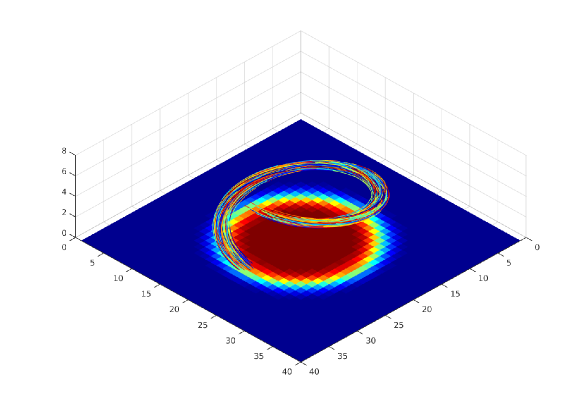
Figure 4: Computing a disk by minimizing the TSC energy. We set $\alpha=10$ and hence the optimal solution of the inpainting problem is given by a disk of radius $r=10$. (a) shows the input image $f$ of size $40\times 40$ pixels together with its inpainting domain indicated by gray pixels and (b)-(e) show the computed solution images $u$ for different numbers of discrete orientations $N_{\theta}$. (f) shows a “stream-line” plot of the averaged Raviart-Thomas vector field $\hat{\sigma}$ on top of a false-color version of the corresponding image $u$.

In the first example, we consider the most basic numerical experiment, which is using TSC energy to compute a disk of a given radius. The aim of this experiment is to investigate the quality of our proposed discretization scheme, in particular when using a different number of discrete orientations. Consider a 2D disk $B(0,r)=\{x\in\mathbb{R}^{2}:|x|\leq r\}$ of radius $r>0$ centered around the origin. The TSC energy of the boundary of the disk $B(0,r)$ is given by

$$\int_{\partial B(0,r)}(1+\alpha^{2}\kappa^{2})d\mathcal{H}^{1}=2\pi(r+\alpha^{2}/r).$$

Here our disk will be represented by its characteristic function $\chi_{B(0,r)}(x)$. We can force the minimizer of the TSC energy to yield a disk using suitable boundary conditions. For example, we can force at least one point inside the disk to be one and at least one point outside the disk to be zero. The following simple computation shows that the minimizer of the TSC energy will be a disk of radius $r=\alpha$, indeed:

$$\int_{\partial B(0,r)}(1+\alpha^{2}\kappa^{2})d\mathcal{H}^{1}=\\ \int_{\partial B(0,r)}\left(\alpha^{2}(\kappa-\frac{1}{\alpha})^{2}+2\alpha\kappa\right)d\mathcal{H}^{1}=\int_{\partial B(0,r)}\alpha^{2}(\kappa-\frac{1}{\alpha})^{2}d\mathcal{H}^{1}+4\pi\alpha,$$

which is minimized if $\kappa=1/r=1/\alpha$ everywhere.

We set up a our optimization problem using a 2D grid of $N_{1}\times N_{2}=40\times 40$ pixels. We will use a different number of discrete orientations $N_{\theta}\in\{4,8,16,32,64\}$ in order to investigate the quality of the approximation depending on $N_{\theta}$. In this and the subsequent experiments, the discretization width of the spatial grid is set to $\delta_{x}=1$ and the discretization width of the angular dimension is set to $\delta_{\theta}=2\pi/N_{\theta}$. The aim of this experiment is to compute a disk of radius $r=10$ pixels. We therefore define an inpainting domain $\mathcal{D}\subseteq\mathcal{I}$ forming a band of 10 pixels width around a disk of radius $r=10$. In this domain we minimize the TSC energy and we use the remaining part of the image as boundary condition. The corresponding data term in our optimization problem (29) is given by

$$G(u)=\sum_{\mathbf{i}\in\mathcal{D}}\iota_{u^{0}_{\mathbf{i}}}(u_{\mathbf{i}}),$$ (32)

where $\iota_{C}$ denotes the indicator function of the convex set $C$. The proximal map for $G(u)$ is given by

$$u=\mathrm{prox}_{\tau G}(v)\;\Longleftrightarrow\;u_{\mathbf{i}}=\begin{cases}v_{\mathbf{i}}&\text{if }\mathbf{i}\in\mathcal{D}\\ u^{0}_{\mathbf{i}}&\text{else}\end{cases},\;\forall\mathbf{i}\in\mathcal{I}.$$ (33)

Figure 4(a) shows the input image $(u^{0}_{\mathbf{i}})_{\mathbf{i}\in\mathcal{I}}$ and the inpainting domain $\mathcal{D}$ is indicated by the gray area.

$N_{\theta}$	$H_{\mathrm{TV}}$ $(2\pi r\approx 62.8319)$	$H_{\mathrm{AC}}$ $(2\pi\approx 6.2832)$	$H_{\mathrm{SC}}$ $(2\pi/r\approx 0.6283)$
4	60.1063	6.3456	1.7504
8	54.8043	6.2847	0.8930
16	58.5041	6.2874	0.7041
32	61.5257	6.2835	0.6448
64	62.9336	6.2835	0.6277

Table 1: Approximating a disk of radius $r=10$. The table shows the values of the computed total variation (TV), absolute curvature (AC), and squared curvature (SC) for a varying number of discrete orientations $N_{\theta}$. In parentheses we also give the values of the respective energies for the true solution. Observe that the squared curvature is approximated well only when using a quite large number of discrete orientations.

In order to quantify the approximation quality of our discretization for a varying number of discrete orientations, we report the total variation (TV), the absolute curvature (AC) and the squared curvature (SC). All three quantities are computed from the averaged field $\hat{\sigma}=\mathcal{A}\sigma$ using the volume-centered based discrete energy

$$H(\hat{\sigma})=\delta_{x}^{2}\delta_{\theta}\sum_{\mathbf{j}\in\mathcal{J}}h(\hat{\sigma}_{\mathbf{j}}),$$

where the function $h$ is one of the three instances:

$$h_{\mathrm{TV}}(\hat{\sigma}_{\mathbf{j}})=\sqrt{(\hat{\sigma}^{1}_{\mathbf{j}})^{2}+(\hat{\sigma}^{2}_{\mathbf{j}})^{2}},\quad h_{\mathrm{AC}}(\hat{\sigma}_{\mathbf{j}})=|\hat{\sigma}^{\theta}_{\mathbf{j}}|,\quad h_{\mathrm{SC}}(\hat{\sigma}_{\mathbf{j}})=\frac{|\hat{\sigma}^{\theta}_{\mathbf{j}}|^{2}}{\sqrt{(\hat{\sigma}^{1}_{\mathbf{j}})^{2}+(\hat{\sigma}^{2}_{\mathbf{j}})^{2}}}.$$

Table 1 details the values of the discrete energies we obtained for different numbers of discrete orientations $N_{\theta}$. From the results, one can see that a higher number of discrete energies generally leads to a better approximation of the true energy. This is particularly true for the value of the squared curvature which seems to be well approximated only when using a quite high number of discrete orientations. The absolute curvature, however seems to be well approximated even when using only a small number of discrete orientations. The reason for this is that the absolute curvature of a smooth curve is easy to approximate by means of a piecewise linear curve.

Figure 4(f) visualizes the averaged Raviart-Thomas vector field $\hat{\sigma}$ of the disk example in case of $N_{\theta}=64$ discrete orientations. Observe that the vector field nicely corresponds to the expected shape of a helix, shown in Figure 1. However, due to diffusive effects of our numerical scheme, the vector field does not perfectly concentrate on a one-dimensional structure.

4.4 Non-smooth level sets

(a) Original image

(b) Input image $u^{0}$

(c) Computed image $u$

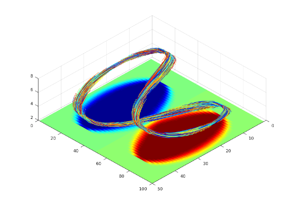
(d) Visualization of the vector field

Figure 5: Effect of convexifying curvature depending energies in the roto-translation space. (a) shows the original image, (b) shows the input image $u^{0}$ of size $100\times 50$ pixels, where gray pixels indicate the inpainting domain. (c) shows the computed solution of minimizing the TSC energy. (d) visualizes the vector field $\hat{\sigma}$ in the roto-translation space. Observe that the twisted $\infty$-shape curve skips the strong curvature at the cusp.

Here we demonstrate a typical effect of our convexification which finds a low-energy solution for an image with non-smooth level sets which should have infinite energy in more standard relaxations [53] of the Elastica energy. Figure 5(a) shows an image of size $N_{1}\times N_{2}=100\times 50$ pixels of a black and a white disk in front of a gray background. Similarly to the inpainting problem of the previous example, we fix only the four small parts of the original image (see Figure 5(b)) and minimize the TSC energy in the inpainting domain $\mathcal{D}$, indicated by the gray area. In this experiment we used $N_{\theta}=64$ discrete orientations and we set $\alpha=17$ to match the radius of the disks. Figure 5(c) shows the computed minimizer of the TSC energy. Observe that the solution $u$ does not yield the expected two disks of the original image but rather drop-like shapes that form a sharp cusp in the middle of the image. Figure 5(b) shows a stream-line representation of the minimizing vector field $\hat{\sigma}$ in the roto-translation space. Inspecting the field, one can immediately see the reason for this behavior. The vector field $\hat{\sigma}$ forms a twisted $\infty$-shape curve which “skips” the strong curvature of the cusp.

4.5 Shape completion

(a) Input image

(b) TAC, $\alpha=15$

(c) TRV, $\alpha=15$

(d) TSC, $\alpha=50$

(e) Input image

(f) TAC, $\alpha=15$

(g) TRV, $\alpha=15$

(h) TSC, $\alpha=10$

(i) Input image

(j) TAC, $\alpha=15$

(k) TRV, $\alpha=15$

(l) TSC, $\alpha=10$

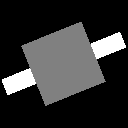
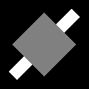
(m) Input images with rotations $0,\pi/8,\pi/4$

(n) TAC, $\alpha=15$

Figure 6: Shape completion for various shapes using total absolute curvature (TAC), total roto-translational variation (TRV) and total squared curvature (TSC). The inpainting domain is indicated by the gray pixels. In the last row we provide results for completing straight lines at different angles.

(a) Original shape

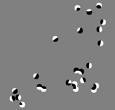
(b) Dipoles

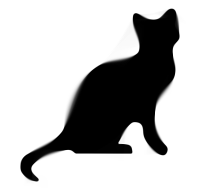
(c) TSC, $\alpha=50$

Figure 7: Computation of “Weickert’s cat” [76]: (a) shows the original shape, (b) depicts the given dipole data and (c) is the result of minimizing the TSC energy in the gray inpaiting domain.

In this section we provide some qualitative results on a number of different shape completion problems. Similar to the previous two examples, we define an inpainting domain $\mathcal{D}$ which is indicated by the gray area and keep the remaining image as boundary condition. Figure 6 shows various input shapes with their inpainting domains and the solutions of minimizing different curvature energies using different settings of the parameter $\alpha$. One can see that while minimizing the TAC energy usually leads to straight connections and sharp corners, TSC leads to a smooth continuation of the boundaries. The TRV energy leads to results which are somewhere in between the results of TAC and TSC. In the last row of Figure 6, we additionally demonstrate the behavior for completing straight lines at different rotations by minimizing the TAC energy. It turns out that our discretization scheme performs quite well for rotations of $0,\pi/4,\pi/2,\ldots$ but leads to more diffusive results for rotations of $\pi/8,3\pi/8,\ldots$. The development of a more isotropic scheme will be subject of future research.

In Figure 7, we show the application to shape completion from dipoles using the original data of “Weickert’s cat” [76]. The input image $u^{0}$ is of size $N_{1}\times N_{2}=400\times 380$ pixels and the inpainting domain $\mathcal{D}$ is again indicated by the gray pixels. In this example we used $N_{\theta}=64$ discrete orientations and the curvature parameter was set to $\alpha=50$. In order to avoid relaxation artifacts (self-intersections) inside the dipoles, we additionally use zero-boundary conditions for the field $\sigma^{1,2}$ within the constant areas of the dipoles. The results show that our numerical scheme can successfully reconstruct the curvilinear shape of the cat from only very little information given by the dipoles. However, we can also observe diffusion artifacts of our numerical scheme, especially if the reconstructed boundaries are relatively long. Sharper results for this kind of problems are usually obtained using sophisticated anisotropic diffusion schemes such as the edge enhancing diffusion (EED) [75, 67]. It would be interesting to understand whether these schemes also minimize an underlying variational energy.

4.6 Shape regularization

(a) Bull fight

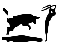
(b) TAC, $\lambda=8$

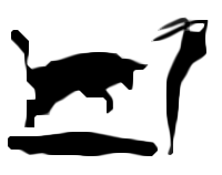
(c) TAC, $\lambda=4$

(d) TAC, $\lambda=2$

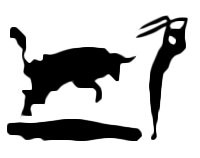
(e) TRV, $\lambda=8$

(f) TRV, $\lambda=4$

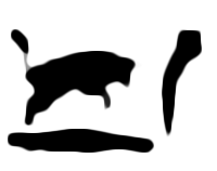
(g) TRV, $\lambda=2$

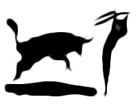
(h) TSC, $\lambda=8$

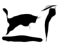
(i) TSC, $\lambda=4$

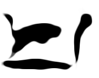
(j) TSC, $\lambda=2$

Figure 8: Shape regularization using curvature regularization. (a) shows the original “Bull fight” image. (b)-(d) show the result of TAC regularization, (e-g) show the result of TRV regularization and (h)-(j) show the result of TSC regularization.

In our next experiment, we apply our curvature based energies for shape regularization. Given an input image $(u^{0}_{\mathbf{i}})_{\mathbf{i}\in\mathcal{I}}$, which is the characteristic function of a given shape, our aim is to compute a simplified (or regularized) shape which is represented by means of a (relaxed) binary image $(u_{\mathbf{i}})_{\mathbf{i}\in\mathcal{I}}$. We make use of a simple linear fidelity term which is frequently used in image segmentation:

$$G(u)=\sum_{\mathbf{i}\in\mathcal{I}}g_{\mathbf{i}},\quad g_{\mathbf{i}}(u_{\mathbf{i}})=u_{\mathbf{i}}w_{\mathbf{i}}+\iota_{[0,1]}(u_{\mathbf{i}}),$$

where $w\in\mathbb{R}^{\mathcal{I}}$ is a force field. For the application to shape regularization we use $w=\lambda(\frac{1}{2}-u^{0})$, where $\lambda>0$ defines the strength of the force field. The proximal map for this data term is easily computed:

$$u=\mathrm{prox}_{\tau G}(v)\;\Longleftrightarrow\;u_{\mathbf{i}}=\max(0,\min(1,v_{\mathbf{i}}-\tau w_{\mathbf{i}})),\;\forall\mathbf{i}\in\mathcal{I}.$$

In Figure 8, we apply TAC, TRV and TSC regularization to regularize the shape of Picasso’s “Bull fight” image. In all three cases, we set $\alpha=10$ and we use different settings of the parameter $\lambda$ to obtain gradually simplified shapes. From the results one can see that TAC regularization yields shapes with relatively straight boundaries and sharp corners. TRV regularization yields smooth shapes but also allows for sharp corners. TSC regularization yields smooth shapes. Observe that whenever it seems energetically preferable, the solution of TSC produces sharp cusps with “hidden” edges to bypass locations of strong curvature, as predicted by the theory [12]. This effect is usually less visible when minimizing the TAC or TRV energies.

4.7 Image inpainting

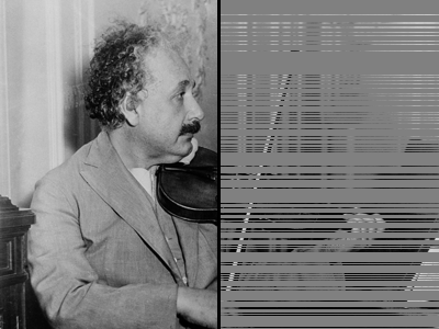
(a) Einstein

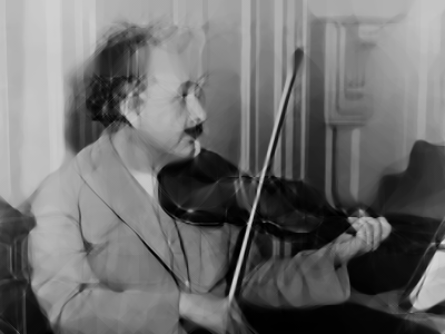
(b) TSC, $\alpha=10$

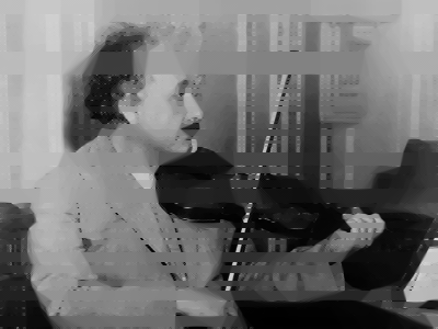
(c) TV, $\alpha=0$

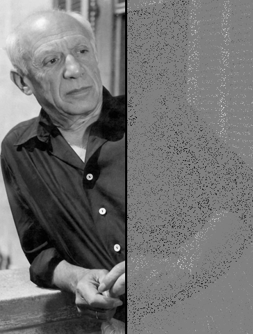
(d) Picasso

(e) TSC, $\alpha=5$

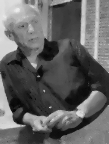
(f) TV, $\alpha=0$

Figure 9: Image inpainting using the proposed curvature-based energies. (a) shows a blend of the original “Einstein” image with its degraded version where we have removed $80\%$ of the lines. (d) shows a blend of the “Picasso” with the version where we have removed $90\%$ of the pixels. (b) is the inpainting result of the “Einstein” and (e) is the inpainting result of the “Picasso” image. For comparison, (c) and (f) show the result of standard TV regularization. Observe that our proposed curvature based regularization leads to significant better inpainting results.

In this section, we apply our proposed curvature energies to the classical problem of image inpainting. Similar to the previous examples, we use the data term (32) with the only difference that the input image $u^{0}$ is now a gray level image. In both examples we used $N_{\theta}=32$ discrete orientations and the curvature parameter was set to $\alpha=15$. Figure 9 shows the results for two different inpainting problems. In the “Einstein” image, we randomly remove $80\%$ lines and in the “Picasso” image we randomly remove $90\%$ of the pixels. In case of the “Einstein” image, we use TSC regularization with $\alpha=10$ and for the “Picasso” we set $\alpha=5$. In case of the “Einstein” image, the gaps a much larger and hence we use a larger value of $\alpha$. For comparison, we also provide results of standard TV regularization, which is equivalent to using $\alpha=0$ in one of the three curvature energies. From the results one can clearly see that curvature regularization leads to significantly better inpainting results. On the downside, we can also observe some artifacts which are caused by our convex representation in the roto-translation space.

4.8 Image denoising

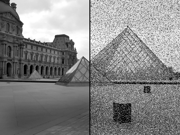
(a) Louvre

(b) TSC, $\alpha=10$, $\lambda=7$

(c) TV, $\alpha=0$, $\lambda=2$

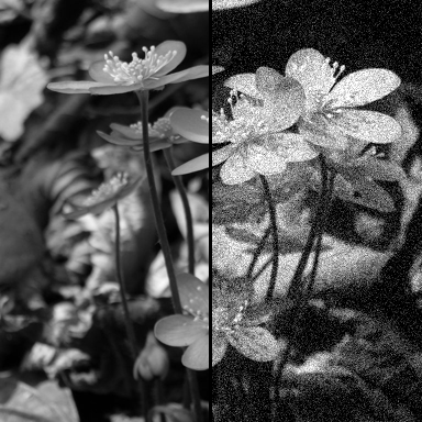
(d) Leberblümchen

(e) TSC, $\alpha=10$, $\lambda=40$

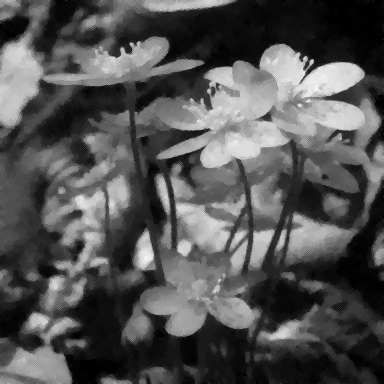
(f) TV, $\alpha=0$, $\lambda=10$

Figure 10: Image denoising using curvature-based regularization. (a) shows the original “Louvre” image blended with a noisy version, where we have added $25\%$ “salt & pepper” noise. (d) shows the clean “Leberblümchen” image together with its noisy variant where we have added zero-mean Gaussian noise with standard deviation $0.1$ (b) and (e) show the result of image denoising using TSC regularization. For comparison we show in (c) and (f) the result when using classical total variation (TV) regularization.

In our last experiments we investigate our curvature energies for the classical problem of image denoising. We investigate two different types of noise: Zero-mean Gaussian noise and impulse noise such as “salt & pepper” noise. For Gaussian noise, it is well-known data a quadratic $\ell_{2}$ data term

$$G(u)=\frac{\lambda}{2}\|{u-f}\|^{2},$$

where $\lambda>0$ is a good data fidelity parameter. The proximal map is given by

$$u=\text{prox}_{\tau G}(v)\;\Longleftrightarrow\;u_{\mathbf{i}}=\frac{v_{i}+\tau\lambda f_{\mathbf{i}}}{1+\tau\lambda},\;\forall\mathbf{i}\in\mathcal{I}.$$

In case of impulse noise, a $\ell_{1}$ data term is more suitable:

$$G(u)=\lambda\|{u-f}\|_{{1}},$$

since it is more robust with respect to outliers. The proximal map for the $\ell_{1}$ data term is given by the classical soft-shrinkage formula

$$u=\text{prox}_{\tau G}(v)\;\Longleftrightarrow\;u_{\mathbf{i}}=f_{\mathbf{i}}+\max(0,|v_{\mathbf{i}}-f_{\mathbf{i}}|-\tau\lambda)\cdot\text{sgn}(v_{\mathbf{i}}-f_{\mathbf{i}}),\;\forall\mathbf{i}\in\mathcal{I}.$$

In Figure 10 we show the results of our curvature-based regularization energies for image denoising. In case of the “Louvre” image we generated the noisy image by adding $25\%$ “salt & pepper” noise. The noisy “Leberblümchen” image was generated by adding zero-mean Gaussian noise with standard deviation $0.1$. In case of Gaussian noise we use a $\ell_{2}$ data term and in case of “salt & pepper” noise we used the $\ell_{1}$ fidelity term. In both cases, we use TSC regularization and the curvature parameter was set to $\alpha=10$. For comparison, we also show the results of standard total variation (TV) denoising, which is obtained from our models by setting $\alpha=0$. One can clearly see that TSC regularization leads to a better preservation of image edges than TV regularization, in particular at small and elongated structures. This effect is more visible in case of “salt & pepper” noise since the $\ell_{1}$ data term leads to a behavior similar to image inpainting, once an outlier is detected.

5 Proof of Theorem 1

This section and the following are devoted to the proof of Theorem 1. We first show a preliminary result which shows that admissible curves (of finite energy) in ${\Omega\times\mathbb{S}^{1}}$ project onto curves in $\Omega$ with bounded energy as well.

5.1 Control of curves

Let $\gamma:[0,L]\to{\Omega\times\mathbb{S}^{1}}$ a rectifiable curve of length $L$ in ${\Omega\times\mathbb{S}^{1}}$, parameterized by its length ($|\dot{\gamma}|=1$ a.e.). We define its energy as

$$\mathcal{E}(\gamma):=\int_{0}^{1}h(\gamma(s),\dot{\gamma(s)})ds$$

and assume that it is finite, which in particular yields that for a.e. $s$,

$$\dot{\gamma}^{x}(s)=|\dot{\gamma}^{x}(s)|(\cos\gamma^{\theta}(s),\sin\gamma^{\theta}(s))^{T}.$$

We consider the projected curve $\gamma^{x}:[0,L]\to\Omega$ (possibly overlapping even if $\gamma$ is simple) and wish to show that the energy $\mathcal{E}$ controls an energy on this curve. First we reparameterize (as usual) the rectifiable curve $\gamma^{x}$ by its length. For this we introduce the length, for $s\in[0,L]$

$$\ell(s):=\int_{0}^{s}|\dot{\gamma}^{x}(t)|dt\in[0,L],$$

which is a $1$-Lipschitz, nondecreasing function. Since clearly for $s^{\prime}>s$ one has $\ell(s)=\ell(s^{\prime})$ if and only if $\dot{\gamma}^{x}(t)=0$ a.e. in $[s,s^{\prime}]$, we also find that $\gamma^{x}(t)=\gamma^{x}(s)$ for all $t\in[s,s^{\prime}]$. This means that (obviously) one can reparameterize $\gamma^{x}$ by defining a curve $\tilde{\gamma}:[0,\ell(L)]\to\Omega$ such that $\tilde{\gamma}(\ell(s))=\gamma^{x}(s)$ for all $s\in[0,L]$. By definition it is clear that $\tilde{\gamma}$ is $1$-Lipschitz, moreover if $l=\ell(s)$ and $l^{\prime}=\ell(s^{\prime})>l$,

$$\frac{\tilde{\gamma}(l^{\prime})-\tilde{\gamma}(l)}{l^{\prime}-l}=\frac{\int_{s}^{s^{\prime}}\dot{\gamma}^{x}(t)dt}{\int_{s}^{s^{\prime}}|\dot{\gamma}^{x}(t)|dt}\stackrel{{\scriptstyle l^{\prime}\to l}}{{\to}}\frac{\dot{\gamma}^{x}(s)}{|\dot{\gamma}^{x}|(s)}=\gamma^{\theta}(s)$$

if $s$ is a Lebesgue point of $\dot{\gamma}^{x}$ where $\dot{\gamma}^{x}(s)\neq 0$. One deduces that for a.e. $l\in[0,\ell(L)]$, $\tilde{\gamma}$ has the tangent vector $\tau(l)=(\cos\theta(l),\sin\theta(l))^{T}$ given by

$$\tau(l)=\dot{\tilde{\gamma}}(l)=\begin{pmatrix}\cos\gamma^{\theta}(s)\\ \cos\gamma^{\theta}(s)\end{pmatrix}$$

where $l=\ell(s)$. Observe that for any smooth $\psi:(0,\ell(L))\to\mathbb{R}$ with compact support one has

$$\int_{0}^{\ell(L)}\dot{\psi}(l)\theta(l)dl=\int_{0}^{L}\dot{\psi}(\ell(s))\theta(\ell(s))\dot{\ell}(s)ds\\ =\int_{0}^{L}\gamma^{\theta}(s)(\psi\circ\ell)^{\prime}(s)ds=-\int_{0}^{L}\dot{\gamma}^{\theta}(s)\psi(\ell(s))ds\leq L\|\psi\|_{C^{0}}$$

which shows that $\theta(l)$ is a $BV$ function, or equivalently that $\tilde{\gamma}$ has a curvature $\kappa=\dot{\theta}$ which is a bounded measure; in particular taking the supremum over $\psi$ with $|\psi|\leq 1$ one finds

$$\int_{0}^{\ell(L)}d|\kappa|(l)\leq\int_{0}^{L}|\dot{\gamma}^{\theta}(s)|ds\leq L.$$

In addition, it follows, given $\psi\in C_{c}^{\infty}(\ell(a),\ell(b))$ with $0\leq a<b\leq L$ that:

$$\int_{\ell(a)}^{\ell(b)}\big{(}-\dot{\psi}(l)\theta(l)-f^{*}(\psi(l))\big{)}dl=\int_{a}^{b}\big{(}-(\psi\circ\ell)^{\prime}(s)\gamma^{\theta}(s)-f^{*}(\psi(\ell(s)))|\dot{\gamma}^{x}(s)|\big{)}ds\\ =\int_{a}^{b}\big{(}\psi(\ell(s))\dot{\gamma}^{\theta}(s)-f^{*}(\psi(\ell(s)))|\dot{\gamma}^{x}(s)|\big{)}ds\leq\int_{a}^{b}h(\gamma(s),\dot{\gamma}(s))ds$$

and taking the supremum one deduces that

$$\int_{\ell(a)}^{\ell(b)}f(\kappa)\leq\int_{a}^{b}h(\gamma(s),\dot{\gamma}(s))ds$$

(where the left-hand side integral in on the open interval and denotes a convex function of a measure). Now, if $\varphi\in C^{0}(\Omega;\mathbb{R}_{+})$ is a bounded, continuous and nonnegative function, one deduces that

$$\int_{0}^{\ell(L)}\varphi(\tilde{\gamma}(l))f(\kappa)=\int_{0}^{\infty}\left(\int_{\{l:\varphi(\tilde{\gamma}(l))>t\}}f(\kappa)\right)dt\\ \leq\int_{0}^{\infty}\left(\int_{\{s:\varphi(\gamma^{x}(s))>t\}}h(\gamma(s),\dot{\gamma}(s))\right)dt$$

and it follows

$$\int_{0}^{\ell(L)}\varphi(\tilde{\gamma}(l))f(\kappa)\leq\int_{0}^{L}\varphi(\gamma^{x}(s))h(\gamma(s),\dot{\gamma}(s))ds.$$ (34)

We now show the following lemma:

Lemma 5.1.

Let $\Gamma\subset\Omega$ be a $C^{2}$ (oriented) curve with tangent $\tau_{\Gamma}$ and curvature $\kappa_{\Gamma}$, ane let and $\gamma:[0,L]\to{\Omega\times\mathbb{S}^{1}}$ be a rectifiable curve. Define $\Gamma^{+}=\{x\in\Gamma:\exists s\in(0,L),\gamma^{x}(s)=x\textup{ and }\dot{\gamma}^{x}(s)\cdot\tau_{\Gamma}\geq 0\}$. Then for any bounded, nonnegative, continuous function $\varphi\in C^{0}(\Omega;\mathbb{R}_{+})$,

$$\int_{\Gamma^{+}}\varphi(x)f(\kappa_{\Gamma})d\mathcal{H}^{1}\leq\int_{0}^{L}\varphi(\gamma^{x}(s))h(\gamma(s),\dot{\gamma}(s))ds.$$ (35)

Proof.

We just need to show that, defining the measure $\kappa$ as before,

$$\int_{\Gamma^{+}}\varphi(x)f(\kappa_{\Gamma})d\mathcal{H}^{1}\leq\int_{0}^{\ell(L)}\varphi(\tilde{\gamma})f(\kappa),$$

and the conclusion will follow from (34).

A first observation is that as $\tau(l)$ defined above is $BV$, it has at most a countable number of jumps and one can cover (up to the jump points) $[0,\ell(L)]$ with an at most countable union of intervals $(a_{i},b_{i})_{i\in I}$ on which $\tau(l)$ is continuous (hence $\tilde{\gamma}$ is a $C^{1}$ curve on $(a_{i},b_{i})$). Moreover, possibly dropping further a finite number of points, one may assume that $|\kappa|(a_{i},b_{i})<\pi$ so that $\gamma^{x}(a_{i},b_{i})$ is a simple curve.

Assume $|\{l\in(a_{i},b_{i})\,:\,\tilde{\gamma}(l)\in\Gamma,\dot{\tilde{\gamma}}(l)\cdot\tau_{\Gamma}\geq 0\}|>0$. Choose such an $l\in(a_{i},b_{i})$, with $x=\tilde{\gamma}(l)\in\Gamma^{+}$, and such that $\tilde{\gamma}$ is differentiable in $l$. We assume in addition that $x$ is a point of ($\mathcal{H}^{1}$-)density one in $\tilde{\gamma}(a_{i},b_{i})\cap\Gamma^{+}$, that $l$ is a Lebesgue point of $\kappa^{a}$, the absolutely continuous part (w.r. the Lebesgue measure) of $\kappa$, and that $\theta(l)$ is approximately differentiable at $l$: for any $\eta>0$,

$$\lim_{\varepsilon\to 0}\frac{1}{2\varepsilon}\left|\left\{s\in(l-\varepsilon,l+\varepsilon):\frac{|\theta(s)-\theta(l)-\kappa^{a}(l)(s-l)|}{|s-l|}ds>\eta\right\}\right|=0.$$

All this is true $\mathcal{H}^{1}$-a.e. in $\tilde{\gamma}(a_{i},b_{i})\cap\Gamma^{+}$, so there is no loss of generality, see for instance [3].

If $\dot{\tilde{\gamma}}(l)\neq\tau_{\Gamma}(x)$, then $x$ must be an isolated point in $\tilde{\gamma}(a_{i},b_{i})\cap\Gamma^{+}$, a contradiction. Hence $\dot{\tilde{\gamma}}(l)=\tau_{\Gamma}(x)$. In the same way, one has that for a.e. $s$ near $l$ such that $\tilde{\gamma}(s)\in\Gamma$, $\dot{\tilde{\gamma}}(s)=\tau_{\Gamma}(\tilde{\gamma}(s))$. For such $s$, one therefore has that

$$\frac{|\theta(s)-\theta(l)-\kappa^{a}(l)(s-l)|}{|s-l|}=\frac{|\theta_{\Gamma}(\tilde{\gamma}(s))-\theta_{\Gamma}(x)-\kappa^{a}(l)(s-l)|}{|s-l|},$$

where $\theta_{\Gamma}$ is the angle between $\begin{pmatrix}1\\ 0\end{pmatrix}$ and $\tau_{\Gamma}$. Using that for such $s$,

$$\theta_{\Gamma}(\tilde{\gamma}(s))-\theta_{\Gamma}(x)=\kappa_{\Gamma}(x)(\tilde{\gamma}(s)-x)\cdot\tau_{\Gamma}(x)+o(|\tilde{\gamma}(s)-x|)\\ =\kappa_{\Gamma}(x)\dot{\tilde{\gamma}}(l)\cdot\tau_{\Gamma}(x)(s-l)+o(|\dot{\tilde{\gamma}}(s)||s-l|)$$

we obtain that for such $s$,

$$\frac{|\theta(s)-\theta(l)-\kappa^{a}(s-l)|}{|s-l|}=|\kappa_{\Gamma}(x)-\kappa^{a}(l)|+o(1)$$

(where $o(1)$ goes to $0$ as $\varepsilon\to 0$). Hence, for $\varepsilon>0$ small and $\eta>0$,

$$\left\{s\in(l-\varepsilon,l+\varepsilon):\frac{|\theta(s)-\theta(l)-\kappa^{a}(l)(s-l)|}{|s-l|}ds>\eta\right\}\\ \supseteq\left\{s\in(l-\varepsilon,l+\varepsilon):\tilde{\gamma}(s)\in\Gamma\textup{ and }|\kappa_{\Gamma}(x)-\kappa^{a}(l)|+o(1)>\eta\right\}$$

In the limit, using that $l$ is a point of density one in the set $\{\tilde{\gamma}(\cdot)\in\Gamma\}$, we obtain that $|\kappa_{\Gamma}(x)-\kappa^{a}(l)|\leq\eta$ and since $\eta$ is arbitrary, $\kappa_{\Gamma}(x)=\kappa^{a}(l)$. Since the intervals $(a_{i},b_{i})$ cover $\mathcal{H}^{1}$-almost all of $[0,\ell(L)]$, we find that this equality holds $\mathcal{H}^{1}$-a.e. in $\Gamma^{+}$.

The thesis of the Lemma easily follows, since

$$\int_{0}^{\ell(L)}\varphi(\tilde{\gamma})f(\kappa)\geq\int_{0}^{\ell(L)}\varphi(\tilde{\gamma})f(\kappa^{a})dx$$

∎

5.2 Decomposition of $\sigma$

Let $u\in BV(\Omega)$ with $F(u)<\infty$. We observe that we can decompose an admissible $\sigma$ (with in particular $\textup{div}\,\sigma=0$) as follows:

$$\sigma=\int_{\mathcal{M}}\lambda d\mu(\lambda),\quad|\sigma|=\int_{\mathcal{M}}|\lambda|d\mu(\lambda),\quad$$ (36)

where $\mu$ is a nonnegative measure on the set of charges $\mathcal{M}$ which is here a shorthand notation for $\mathcal{M}({\Omega\times\mathbb{S}^{1}};\mathbb{R}^{3})$: see Appendix B which discusses the results of Smirnov in [73].

Lemma 5.2.

Assume (36) holds. Then for any $g(\xi,p)$ nonnegative, continuous, convex and one-homogeneous in its second argument,

$$\int_{{\Omega\times\mathbb{S}^{1}}}g(\xi,\sigma)=\int_{\mathcal{M}}\left(\int_{{\Omega\times\mathbb{S}^{1}}}g(\xi,\lambda)\right)d\mu(\lambda).$$ (37)

Proof.

For $\rho>0$ we define $\Omega_{\rho}=\{x\in\Omega:\textup{dist}\,(x,\partial\Omega)>\rho\}$. We let for $\rho>0$, $\varepsilon\in(0,\rho)$ and $\xi\in{\Omega_{2\rho}\times\mathbb{S}^{1}}$

$$f_{\rho,\varepsilon}(\xi)=\begin{cases}\frac{\sigma({\Omega_{3\rho}\times\mathbb{S}^{1}}\cap\overline{B}(\xi,\rho))}{|\sigma|(B(\xi,\rho+\varepsilon))}&\textup{ if }|\sigma|(B(\xi,\rho+\varepsilon))>0\,,\\ 0&\textup{ else.}\end{cases}$$

We also let $f_{\rho,\varepsilon}(\xi)=0$ if $\xi\in{\Omega\times\mathbb{S}^{1}}\setminus{\Omega_{2\rho}\times\mathbb{S}^{1}}$: remark then that $f_{\rho,\varepsilon}\in C_{c}^{0}({\Omega\times\mathbb{S}^{1}};B(0,1))$ and that

$$f_{\rho}(\xi):=\lim_{\varepsilon\to 0}f_{\rho,\varepsilon}(\xi)=\begin{cases}\frac{\sigma({\Omega_{3\rho}\times\mathbb{S}^{1}}\cap\overline{B}(\xi,\rho))}{|\sigma|(\overline{B}(\xi,\rho))}&\textup{ if }\xi\in\Omega_{2\rho}\times\mathbb{S}^{1},\,|\sigma|(\overline{B}(\xi,\rho))>0\,,\\ 0&\textup{ else.}\end{cases}$$

By (37) we have for any $\varphi\in C_{c}^{0}({\Omega\times\mathbb{S}^{1}};\mathbb{R}_{+})$:

$$\int_{{\Omega\times\mathbb{S}^{1}}}\varphi(|\sigma|-f_{\rho,\varepsilon}\cdot\sigma)=\int_{\mathcal{M}}\left(\int_{{\Omega\times\mathbb{S}^{1}}}\varphi(|\lambda|-f_{\rho,\varepsilon}\cdot\lambda)\right)d\mu.$$

Observe that

$$\int_{{\Omega\times\mathbb{S}^{1}}}\varphi(|\lambda|-f_{\rho,\varepsilon}\cdot\lambda)\\ =\int_{{\Omega\times\mathbb{S}^{1}}}\varphi\left(|\lambda|-f_{\rho}\cdot\lambda\right)\frac{{|\sigma|(\overline{B}(\xi,\rho))}}{{|\sigma|(B(\xi,\rho+\varepsilon))}}+\int_{{\Omega\times\mathbb{S}^{1}}}\varphi\frac{|\sigma|(B(\xi,\rho+\varepsilon)\setminus\overline{B}(\xi,\rho))}{|\sigma|(B(\xi,\rho+\varepsilon))}|\lambda|$$

and using the monotone convergence theorem, we can send $\varepsilon\to 0$ and deduce that

$$\int_{{\Omega\times\mathbb{S}^{1}}}\varphi(|\sigma|-f_{\rho}\cdot\sigma)=\int_{\mathcal{M}}\left(\int_{{\Omega\times\mathbb{S}^{1}}}\varphi(|\lambda|-f_{\rho}\cdot\lambda)\right)d\mu.$$ (38)

Then, thanks to Radon-Nikodym’s derivation theorem (and Lebesgue’s convergence theorem),

$$\lim_{\rho\to 0}\int_{{\Omega\times\mathbb{S}^{1}}}\varphi(|\sigma|-f_{\rho}\cdot\sigma)=0.$$

Observe that all the integrands in (38) are nonnegative. Let $\varphi_{n}$ be a nondecreasing sequence of compactly supported nonnegative smooth functions which converges to $1$. Then one can build a subsequence $\rho_{n}\downarrow 0$ such that

$$\sum_{n}\int_{{\Omega\times\mathbb{S}^{1}}}\varphi_{n}(|\sigma|-f_{\rho_{n}}\cdot\sigma)<+\infty,$$

so that

$$\int_{\mathcal{M}}\left(\int_{{\Omega\times\mathbb{S}^{1}}}\sum_{n}\varphi_{n}(|\lambda|-f_{\rho_{n}}\cdot\lambda)\right)d\mu<+\infty.$$

It follows that there exists a set $E\subset\mathcal{M}$ with $\mu(E)=0$ such that if $\lambda\not\in E$,

$$\lim_{n}\int_{{\Omega\times\mathbb{S}^{1}}}\varphi_{n}(|\lambda|-f_{\rho_{n}}\cdot\lambda)=0$$

and $f_{\rho_{n}}\cdot\frac{\lambda}{|\lambda|}\to 1$ $|\lambda|$-a.e. in ${\Omega\times\mathbb{S}^{1}}$ (using $|\lambda|-f_{\rho_{n}}\cdot\lambda=|\lambda|(1-f_{\rho_{n}}\cdot\frac{\lambda}{|\lambda|})\geq 0$). Using $|f_{\rho_{n}}-\frac{\lambda}{|\lambda|}|^{2}=|f_{\rho_{n}}^{2}|+1-2f_{\rho_{n}}\cdot\frac{\lambda}{|\lambda|}\leq 2(1-f_{\rho_{n}}\cdot\frac{\lambda}{|\lambda|})$ it follows that $f_{\rho_{n}}\to\frac{\lambda}{|\lambda|}$, $|\lambda|$-a.e.

Let $g:({\Omega\times\mathbb{S}^{1}})\times\mathbb{R}^{3}\to\mathbb{R}$ be a continuous, nonegative, and convex one-homogeneous function in its second argument. Then as before for $\varphi\in C_{c}^{0}({\Omega\times\mathbb{S}^{1}};\mathbb{R}_{+})$

$$\int_{{\Omega\times\mathbb{S}^{1}}}\varphi(\xi)g(\xi,f_{\rho,\varepsilon}(\xi))|\sigma|=\int_{\mathcal{M}}\int_{{\Omega\times\mathbb{S}^{1}}}\varphi(\xi)g(\xi,f_{\rho,\varepsilon})|\lambda|d\mu$$

and since $g(\xi,f_{\rho,\varepsilon}(\xi))=(|\sigma|(\overline{B}(\xi,\rho))/|\sigma|(B(\xi,\rho+\varepsilon)))g(\xi,f_{\rho}(\xi))\uparrow g(\xi,f_{\rho}(\xi))$ as $\varepsilon\downarrow 0$, the monotone convergence theorem yields that

$$\int_{{\Omega\times\mathbb{S}^{1}}}\varphi g(\xi,f_{\rho})|\sigma|=\int_{\mathcal{M}}\int_{{\Omega\times\mathbb{S}^{1}}}\varphi g(\xi,f_{\rho})|\lambda|d\mu.$$

Using Lebesgue’s theorem, we have

$$\lim_{\rho\to 0}\int_{{\Omega\times\mathbb{S}^{1}}}\varphi(\xi)g(\xi,f_{\rho}(\xi))|\sigma|=\int_{{\Omega\times\mathbb{S}^{1}}}\varphi(\xi)g(\xi,\tfrac{\sigma}{|\sigma|}(\xi))|\sigma|=\int_{{\Omega\times\mathbb{S}^{1}}}\varphi(\xi)g(\xi,\sigma).$$

On the other hand, we know that if $\lambda\not\in E$, still thanks to Lebesgue’s theorem,

$$\lim_{n}\int_{{\Omega\times\mathbb{S}^{1}}}\varphi(\xi)g(\xi,f_{\rho_{n}}(\xi))|\lambda|=\int_{{\Omega\times\mathbb{S}^{1}}}\varphi(\xi)g(\xi,\tfrac{\lambda}{|\lambda|}(\xi))|\lambda|=\int_{{\Omega\times\mathbb{S}^{1}}}\varphi g(\xi,\lambda).$$

We invoke one last time Lebesgue’s theorem to deduce that (for all nonnegative test function $\varphi$)

$$\lim_{n}\int_{\mathcal{M}}\left(\int_{{\Omega\times\mathbb{S}^{1}}}\varphi(\xi)g(\xi,f_{\rho_{n}}(\xi))|\lambda|\right)d\mu=\int_{\mathcal{M}}\left(\int_{{\Omega\times\mathbb{S}^{1}}}\varphi g(\xi,\lambda)\right)d\mu.$$

We deduce (37). ∎

Corollary 5.3.

Let $\sigma$ be admissible for problem (6), and assume it is decomposed as in (36). Then $\mu$-a.e. measure $\lambda$ satisfies

$$\frac{\lambda}{|\lambda|}\cdot\theta\geq 0\,,\frac{\lambda}{|\lambda|}\cdot\theta^{\perp}=0\,\textit{a.e.}~{}\textup{in }{\Omega\times\mathbb{S}^{1}}$$

Proof.

Apply the Lemma with $g(\xi,p)=(\theta\cdot p)^{-}$ and then with $g(\xi,p)=|\theta^{\perp}\cdot p|$. ∎

Corollary 5.4.

Let $\sigma$ be admissible for problem (6), and assume it is decomposed as in (36). Let $h$ be defined as in (3), and $\varphi\in C_{c}^{0}(\Omega)$ a nonnegative test function. Then

$$\int_{{\Omega\times\mathbb{S}^{1}}}\varphi(x)h(\theta,\sigma)=\int_{\mathcal{M}}\left(\int_{{\Omega\times\mathbb{S}^{1}}}\varphi(x)h(\theta,\lambda)\right)d\mu(\lambda).$$ (39)

Proof.

This is a consequence of Lemma 5.2, however now $h$ can take the value $+\infty$. We simply observe that if we let, for $\varepsilon>0$,

$$h_{\varepsilon}(\theta,p):=\min_{q\in\mathbb{R}^{3}}h(\theta,q)+\frac{1}{\varepsilon}|p-q|$$

then $h_{\varepsilon}$ is $(1/\varepsilon)$-Lipschitz, convex, one-homogeneous in the second variable, and continuous (and hence also $(\xi,p)=((x,\theta),p)\mapsto\varphi(x)h_{\varepsilon}(\theta,p)$). Hence (37) yields

$$\int_{{\Omega\times\mathbb{S}^{1}}}\varphi(x)h_{\varepsilon}(\theta,\sigma)=\int_{\mathcal{M}}\left(\int_{{\Omega\times\mathbb{S}^{1}}}\varphi(x)h_{\varepsilon}(\theta,\lambda)\right)d\mu(\lambda).$$

The results follows from the monotone convergence theorem. ∎

5.3 Conclusion: proof of Theorem 1

We can now complete the proof of Theorem 1. We consider $E$ a $C^{2}$ set. First, if $\gamma(t):[0,1]\to\Omega$ is an oriented parameterization of (the closure of) $\partial E\cap\Omega$, (assuming it is connected, otherwise one needs to introduce a curve for each connected component), one can define in ${\Omega\times\mathbb{S}^{1}}$ the curve $\lambda(t)=(\gamma(t),\theta(t))$ where $\theta(t)$ is defined by $\lambda(t)=|\gamma^{\prime}(t)|(\cos\theta(t),\sin\theta(t))^{T}$. We then let $\Gamma=\lambda([0,1])\cap{\Omega\times\mathbb{S}^{1}}$ and $\sigma=\tau_{\Gamma}\mathcal{H}^{1}{{\mathchoice{\>\hbox{\vrule width=0.2pt\vbox to7.0pt{\vfill\hrule width=7.0pt,height=0.2pt}}\>}{\>\hbox{\vrule width=0.2pt\vbox to7.0pt{\vfill\hrule width=7.0pt,height=0.2pt}}\>}{\,\hbox{\vrule width=0.2pt\vbox to5.0pt{\vfill\hrule width=5.0pt,height=0.2pt}}\,}{\,\hbox{\vrule width=0.2pt\vbox to3.35pt{\vfill\hrule width=3.35pt,height=0.2pt}}\,}}}\Gamma$. Then, $\sigma$ is admissible for (6) with $u=\chi_{E}$, and one finds that

$$F(\chi_{E})\leq\int_{{\Omega\times\mathbb{S}^{1}}}h(\theta,\sigma)=\int_{\partial E\cap\Omega}f(\kappa_{E})d\mathcal{H}^{1}.$$

We need therefore to prove the reverse inequality. Let $\sigma$ be admissible for (6). Thanks to [73, Theorem A] (cf Appendix B, eq. (59)), one can decompose $\sigma$ as

$$\sigma=\int_{\mathfrak{C}_{1}}\lambda d\mu(\lambda),\quad|\sigma|=\int_{\mathfrak{C}_{1}}|\lambda|d\mu(\lambda),$$

where $\lambda$ are of the form

$$\lambda_{\gamma}=\tau_{\gamma}\mathcal{H}^{1}{{\mathchoice{\>\hbox{\vrule width=0.2pt\vbox to7.0pt{\vfill\hrule width=7.0pt,height=0.2pt}}\>}{\>\hbox{\vrule width=0.2pt\vbox to7.0pt{\vfill\hrule width=7.0pt,height=0.2pt}}\>}{\,\hbox{\vrule width=0.2pt\vbox to5.0pt{\vfill\hrule width=5.0pt,height=0.2pt}}\,}{\,\hbox{\vrule width=0.2pt\vbox to3.35pt{\vfill\hrule width=3.35pt,height=0.2pt}}\,}}}\gamma$$

for rectifiable (possibly closed) curves $\gamma\subset{\Omega\times\mathbb{S}^{1}}$ of length at most one.

Equation (39) is valid for this decomposition and shows that for any $\varphi\in C_{c}^{0}(\Omega;[0,1])$,

$$\int_{{\Omega\times\mathbb{S}^{1}}}\varphi(x)h(\theta,\sigma)=\int_{\mathfrak{C}_{1}}\left(\int_{\gamma}\varphi(x)h(\theta,\tau_{\gamma})d\mathcal{H}^{1}\right)d\mu(\lambda_{\gamma}).$$ (40)

Now, for any $\psi\in C_{c}^{0}(\Omega;\mathbb{R}^{2})$, one has

$$\int_{{\Omega\times\mathbb{S}^{1}}}(\psi,0)^{T}\cdot\sigma=\int_{\Omega}\psi\cdot Du^{\perp}=\int_{\partial\Omega}\psi\cdot\tau_{E}d\mathcal{H}^{1}$$ (41)

where $\tau_{E}$ is a tangent vector to $\partial E$ (oriented with $E$ on the left-hand side and $E^{c}$ on the right-hand side).

Let us introduce the signed distance function $d_{E}(x)=\textup{dist}\,(x,\Omega\setminus E)-\textup{dist}\,(x,E)$ which is $C^{2}$ in a neighborhood of $\partial E$ and is such that $\nabla d_{E}=\nu_{E}$ (the inner normal) on $\partial\Omega$ and $\Delta d_{E}=-\kappa_{E}$ (we assume the curvature is nonnegative where the set is convex). If we consider, for $\varepsilon>0$, a test function of the form

$$\psi(x)=(\nabla d_{E}(x))^{\perp}\left(1-\frac{|d_{E}(x)|}{\varepsilon}\right)^{+}\varphi(x),$$

with $\varphi\in C_{c}^{0}(\Omega)$, (41) yields

$$\int_{\partial E}\varphi(x)d\mathcal{H}^{1}=\int_{{\Omega\times\mathbb{S}^{1}}}(\psi,0)^{T}\cdot\sigma\\ =\int_{\mathfrak{C}_{1}}\left(\int_{\gamma}\varphi(x)\left(1-\frac{|d_{E}(x)|}{\varepsilon}\right)^{+}((\nabla d_{E}(x))^{\perp},0)^{T}\cdot\tau_{\gamma}(x,\theta)d\mathcal{H}^{1}\right)d\mu(\lambda_{\gamma}).$$

Sending $\varepsilon\to 0$ we find that

$$\int_{\partial E}\varphi(x)d\mathcal{H}^{1}=\int_{\mathfrak{C}_{1}}\left(\int_{\gamma\cap(\partial E\times\mathbb{S}^{1})}\varphi\,(\tau_{E},0)^{T}\cdot\tau_{\gamma}d\mathcal{H}^{1}\right)d\mu(\lambda_{\gamma}).$$

Now, we can choose $\varphi$ of the form $\varphi(x)f(\kappa_{E}(x))$, with $\varphi\in C_{c}^{0}(\Omega;[0,1])$, assuming $f$ is finite-valued. We obtain that

$$\int_{\partial E}\varphi f(\kappa_{E})d\mathcal{H}^{1}=\int_{\mathfrak{C}_{1}}\left(\int_{\gamma\cap(\partial E\times\mathbb{S}^{1})}\varphi f(\kappa_{E})\tau_{E}\cdot\tau^{x}_{\gamma}d\mathcal{H}^{1}\right)d\mu(\lambda_{\gamma}).$$ (42)

Given the rectifiable curve $\gamma$, one has that

$$\int_{\gamma\cap(\partial E\times\mathbb{S}^{1})}\varphi f(\kappa_{E})\tau_{E}\cdot\tau^{x}_{\gamma}d\mathcal{H}^{1}\leq\int_{\Pi(\gamma)\cap\partial E}\varphi f(\kappa_{E})(\tau_{E}\cdot\tau_{\Pi(\gamma)})^{+}d\mathcal{H}^{1}\\ \leq\int_{{\Omega\times\mathbb{S}^{1}}}\varphi(x)h(\theta,\lambda_{\gamma})$$ (43)

thanks to (35) in Lemma 5.1. Then, (40), (42) and (43) yield

$$\int_{\partial E}\varphi(x)f(\kappa_{E})d\mathcal{H}^{1}\leq\int_{{\Omega\times\mathbb{S}^{1}}}\varphi(x)h(\theta,\sigma)$$

and Theorem 1 is easily deduced. In case $f$ takes the value $+\infty$, then we first approximates $f$ with a finite-valued function from below (replacing $f$ with $\min_{t^{\prime}}f(t^{\prime})+|t-t^{\prime}|/\varepsilon$ for $\varepsilon>0$ small), and once the inequality is established for this function we send $\varepsilon\to 0$, so that (9) also holds.

Appendix A Consistency of the discretization

In this appendix, we study the consistency of the discrete approximation of the problem which is used in Section 4.

A.1 Preliminary results

Let us introduce, for $(s,t)\in\mathbb{R}^{2}$,

$$\bar{h}(s,t)=\begin{cases}sf(t/s)&\textup{ if }s>0,\\ f^{\infty}(t)&\textup{ if }s=0,\\ +\infty&\textup{else,}\end{cases}$$

which is such that

$$\bar{h}(s,t)=\sup_{a+f^{*}(b)\leq 0}as+bt.$$

Observe that if the convex function $f$ is differentiable, then for $s>0$, $\partial_{s}\bar{h}(s,t)=f(t/s)-(t/s)f^{\prime}(t/s)\leq f(0)$.

Consider a vector-valued measurable function $\sigma(\theta)=(\lambda(\theta)\underline{\theta},\mu(\theta))$ where $\lambda\geq 0$. Let then $\bar{\theta}\in\mathbb{S}^{1}$, $\delta_{\theta}>0$ and

$$\bar{\sigma}=\frac{1}{\delta_{\theta}}\int_{\bar{\theta}-\frac{\delta_{\theta}}{2}}^{\bar{\theta}+\frac{\delta_{\theta}}{2}}\sigma(\theta)d\theta.$$

We first observe that

$$\bar{\sigma}\cdot\bar{}\underline{\theta}=\frac{1}{\delta_{\theta}}\int_{\bar{\theta}-\frac{\delta_{\theta}}{2}}^{\bar{\theta}+\frac{\delta_{\theta}}{2}}\lambda(\theta)\underline{\theta}\cdot\bar{}\underline{\theta}d\theta\in\left[\bar{\lambda}\cos\tfrac{\delta_{\theta}}{2},\bar{\lambda}\right]$$

where

$$\bar{\lambda}=\frac{1}{\delta_{\theta}}\int_{\bar{\theta}-\frac{\delta_{\theta}}{2}}^{\bar{\theta}+\frac{\delta_{\theta}}{2}}\lambda(\theta)d\theta.$$

Assuming $f$ is smooth, it follows that

$$\bar{h}\Big{(}\tfrac{\bar{\sigma}\cdot\bar{}\underline{\theta}}{\cos\frac{\delta_{\theta}}{2}},\bar{\sigma}^{\theta}\Big{)}=\bar{h}(\bar{\lambda},\bar{\sigma}^{\theta})+\int_{0}^{1}\partial_{s}\bar{h}\Big{(}\bar{\lambda}+s\Big{(}\tfrac{\bar{\sigma}\cdot\bar{}\underline{\theta}}{\cos\frac{\delta_{\theta}}{2}}-\bar{\lambda}\Big{)},\bar{\sigma}^{\theta}\Big{)}\Big{(}\tfrac{\bar{\sigma}\cdot\bar{}\underline{\theta}}{\cos\frac{\delta_{\theta}}{2}}-\bar{\lambda}\Big{)}ds\\ \leq\bar{h}(\bar{\lambda},\bar{\sigma}^{\theta})+f(0)\bar{\lambda}\frac{1-\cos\frac{\delta_{\theta}}{2}}{\cos\frac{\delta_{\theta}}{2}}.$$

Using that $\bar{h}$ is $1$-homogeneous and that $\bar{h}(s,t)\geq\gamma\sqrt{s^{2}+t^{2}}$, it follows

$$\bar{h}\big{(}\bar{\sigma}\cdot\bar{}\underline{\theta},\cos\tfrac{\delta_{\theta}}{2}\bar{\sigma}^{\theta}\big{)}\leq\cos\tfrac{\delta_{\theta}}{2}\bar{h}(\bar{\lambda},\bar{\sigma}^{\theta})+\big{(}1-\cos\tfrac{\delta_{\theta}}{2}\big{)}\frac{f(0)}{\gamma}\bar{h}(\bar{\lambda},\bar{\sigma}^{\theta})\\ \leq\left(1+\frac{\delta_{\theta}^{2}}{4}(f(0)/\gamma-1)\right)\bar{h}(\bar{\lambda},\bar{\sigma}^{\theta})$$

if $\delta_{\theta}$ is small enough. Observe that if $f$ is not smooth, this still holds by approximation. It follows, thanks to Jensen’s inequality and the fact that $h(\theta,\sigma)=\bar{h}(\lambda,\sigma^{\theta})$ for all $\theta$, that provided $\delta_{\theta}$ is small enough (not depending on anything)

$$\bar{h}\big{(}\bar{\sigma}\cdot\bar{}\underline{\theta},\cos\tfrac{\delta_{\theta}}{2}\bar{\sigma}^{\theta}\big{)}\leq(1+C{\delta_{\theta}^{2}})\frac{1}{\delta_{\theta}}\int_{\bar{\theta}-\frac{\delta_{\theta}}{2}}^{\bar{\theta}+\frac{\delta_{\theta}}{2}}h(\theta,\sigma(\theta))d\theta,$$ (44)

where the constant $C=(f(0)/\gamma-1)/4$ only depends on the function $f$.

Remark A.1.

If $\sigma$ is a bounded measure such that $\int h(\theta,\sigma)<+\infty$, then (44) still holds with now all integrals and averages replaced with integrals over $[\bar{\theta}-\delta_{\theta}/2,\bar{\theta}+\delta_{\theta}/2)$. Indeed, in this case, approximating $\sigma$ with smooth measures by convolution one easily deduces that it holds for almost all $\bar{\theta}$ (whenever $|\sigma|(\{\bar{\theta}-\delta_{\theta}/2,\bar{\theta}+\delta_{\theta}/2\})=0$). Then, for the other values, it is enough to find a sequence $\varepsilon_{n}>0$ with $\varepsilon_{n}\downarrow 0$ such that the result holds for $\bar{\theta}-\varepsilon_{n}$ and use the fact that for any bounded measure $\mu$,

$$\lim_{n\to\infty}\mu([\bar{\theta}-\varepsilon_{n}-\tfrac{\delta_{\theta}}{2},\bar{\theta}-\varepsilon_{n}+\tfrac{\delta_{\theta}}{2}))=\mu([\bar{\theta}-\tfrac{\delta_{\theta}}{2},\bar{\theta}+\tfrac{\delta_{\theta}}{2}))$$

as $\mu([\theta-\varepsilon_{n},\theta))\to 0$ as $n\to\infty$ for any $\theta\in\mathbb{S}^{1}$.

We can now show the following lemma:

Lemma A.2.

Let $\delta_{x},\delta_{\theta}>0$ small enough, $\sigma\in\mathcal{M}^{1}({\Omega\times\mathbb{S}^{1}};\mathbb{R}^{3})$ with $\textup{div}\,\sigma=0$ and such that $\int_{{\Omega\times\mathbb{S}^{1}}}h(\theta,\sigma)<\infty$. Define, for $(\bar{x},\bar{\theta})\in{\Omega\times\mathbb{S}^{1}}$,

$$S=\left[\bar{x}_{1}-\tfrac{\delta_{x}}{2},\bar{x}_{1}+\tfrac{\delta_{x}}{2}\right)\times\left[\bar{x}_{2}-\tfrac{\delta_{x}}{2},\bar{x}_{2}+\tfrac{\delta_{x}}{2}\right)$$

and

$$\bar{\sigma}=\frac{1}{\delta_{x}^{2}\delta_{\theta}}\sigma(S\times[\bar{\theta}-\tfrac{\delta_{\theta}}{2},\bar{\theta}+\tfrac{\delta_{\theta}}{2})).$$

Then,

$$\bar{h}(\bar{\sigma}\cdot\bar{}\underline{\theta},\cos\tfrac{\delta_{\theta}}{2}\bar{\sigma}^{\theta})\leq\frac{1+C\delta_{\theta}^{2}}{\delta_{x}^{2}\delta_{\theta}}\int_{S\times[\bar{\theta}-\frac{\delta_{\theta}}{2},\bar{\theta}+\frac{\delta_{\theta}}{2})}h(\theta,\sigma)$$ (45)

where $C$ depends only on $f$. Moreover, $\bar{\sigma}^{x}/|\bar{\sigma}|$ lies in the cone $\mathbb{R}_{+}(\underline{\theta-\delta_{\theta}/2})+\mathbb{R}_{+}(\underline{\theta+\delta_{\theta}/2})$.

Proof.

If we introduce the (averaged) marginal $\sigma^{\prime}\in\mathcal{M}^{1}(\mathbb{S}^{1};\theta)$ defined by $\int_{\mathbb{S}^{1}}\psi\sigma^{\prime}=\frac{1}{\delta_{x}^{2}}\int_{S\times\mathbb{S}^{1}}\psi\sigma$ for all $\psi\in C^{0}(\mathbb{S}^{1})$, then one observes that

$$\bar{\sigma}=\frac{1}{\delta_{\theta}}\sigma^{\prime}({[\bar{\theta}-\tfrac{\delta_{\theta}}{2},\bar{\theta}+\tfrac{\delta_{\theta}}{2})})$$

and

$$\int_{[\bar{\theta}-\frac{\delta_{\theta}}{2},\bar{\theta}+\frac{\delta_{\theta}}{2})}h(\theta,\sigma^{\prime})\leq\int_{S\times[\bar{\theta}-\frac{\delta_{\theta}}{2},\bar{\theta}+\frac{\delta_{\theta}}{2})}h(\theta,\sigma).$$

This follows by a disintegration argument and using Jensen’s inequality in each “slice” corresponding to a fixed value of $\theta$. The result then follows from (44), together with Remark A.1.

The last statement comes from the fact that $\sigma_{x}$ is the average of measures all contained in the cone, which is convex. ∎

Consider now a measure $\sigma$ admissible for some function $u$, and assume that $\sigma$ is “smooth” in $x$: we assume for instance that it is the result of a convolution $\rho_{\varepsilon}*\sigma^{\prime}$ for some $\sigma^{\prime}$ admissible (possibly extended in a larger domain), with $\rho_{\varepsilon}(x)$ a rotationally symmetric mollifier, as in the proof of Proposition 3.1. In this case, $x\mapsto\sigma$ can be seen as a $\mathcal{M}^{1}(\mathbb{S}^{1};\mathbb{R}^{3})$-valued smooth function.

Consider $(\bar{x},\bar{\theta})\in{\Omega\times\mathbb{S}^{1}}$, $\delta_{x},\delta_{\theta}$ small, and define in the volume $V=S\times[\bar{\theta}-\delta_{\theta}/2,\bar{\theta}+\delta_{\theta}/2)$ the average $\bar{\sigma}$ as before and the “Raviart-Thomas” approximation of $\sigma$ defined by the average fluxes through the 6 facets of $V$ (linearly extended inside the volume, as in eq. 21). There are several ways to define this properly, at least for all $\bar{\theta}$ but a countable number. In our case, one can disintegrate the measure in ${\Omega\times\mathbb{S}^{1}}$ as $\sigma=\sigma_{\theta}d\mu$ where $\mu$ is a bounded positive measure in $\mathbb{S}^{1}$ and for all $\theta$, $\sigma_{\theta}\in C^{\infty}(\Omega)$. Then

$$\tau^{1}_{\pm}=\frac{1}{\delta_{x}\delta_{\theta}}\int_{[\bar{\theta}-\delta_{\theta}/2,\bar{\theta}+\delta_{\theta}/2)}\left(\int_{\bar{x}_{2}-\frac{\delta_{x}}{2}}^{\bar{x}_{2}+\frac{\delta_{x}}{2}}\sigma^{1}_{\theta}(\bar{x}_{1}\pm\tfrac{\delta_{x}}{2},x_{2},\theta)dx_{2}\right)\mu,$$

$$\tau^{2}_{\pm}=\frac{1}{\delta_{x}\delta_{\theta}}\int_{[\bar{\theta}-\delta_{\theta}/2,\bar{\theta}+\delta_{\theta}/2)}\left(\int_{\bar{x}_{1}-\frac{\delta_{x}}{2}}^{\bar{x}_{1}+\frac{\delta_{x}}{2}}\sigma^{1}_{\theta}(x_{1},\bar{x}_{2}\pm\tfrac{\delta_{x}}{2},\theta)dx_{1}\right)\mu.$$

To define the vertical fluxes $\tau^{\theta}_{\pm}$ we assume in addition that $\mu(\{\bar{\theta}\pm\delta_{\theta}/2\})=0$ (which is true for all values but a countable number). In this case, observe that if $\phi\in C_{c}^{1}(\mathring{S}\times\{\theta=-\delta_{\theta}/2\})$, it can be extended into a $C^{1}$ function in $V$ vanishing near the 5 other boundaries, and then

$$\int_{V}\nabla\phi\cdot\sigma$$

defines a measure $\tilde{\tau}^{\theta}_{-}$ on $\mathring{S}\times\{\theta=-\delta_{\theta}/2\}$. Then one simply let $\tau^{\theta}_{-}=\tilde{\tau}^{\theta}_{-}(\mathring{S}\times\{\theta=-\delta_{\theta}/2\})/\delta_{x}^{2}$. The value $\tau^{\theta}_{+}$ is defined in the same way. The assumption that $\mu(\{\bar{\theta}-\delta_{\theta}/2\})=0$ guarantees that the same construction from below will build the same measure and the same value, and that one actually has $(\tau^{1}_{+}-\tau^{1}_{-}+\tau^{2}_{+}-\tau^{2}_{-})/\delta_{x}+(\tau^{\theta}_{+}-\tau^{\theta}_{-})/\delta_{\theta}=0$.

We can show the following lemma.

Lemma A.3.

Let $\tau=(\tau^{1}_{a},\tau^{2}_{b},\tau^{\theta}_{c})^{T}$ for any $(a,b,c)\in\{-,+\}^{3}$. Then, for all $\bar{\theta}$ but a countable number,

$$\delta_{x}^{2}\delta_{\theta}|\tau-\bar{\sigma}|\leq\sqrt{\delta_{x}^{2}+\delta_{\theta}^{2}}\int_{V}|\partial_{1}\sigma^{1}|+|\partial_{2}\sigma^{2}|.$$ (46)

Proof.

We prove the result for $(a,b,c)=(-,-,-)$, the proof in the other cases being identical. We first assume that $\sigma$ is also $C^{1}$ in $\theta$ (which can be achieved by convolution). In this case, one has for all $(x_{1},x_{2},\theta)\in V$,

$$\sigma^{1}(\bar{x}_{1}-\tfrac{\delta_{x}}{2},x_{2},\theta)=\sigma^{1}(x_{1},x_{2},\theta)-\int_{\bar{x}_{1}-\frac{\delta_{x}}{2}}^{x_{1}}\partial_{1}\sigma^{1}(s,x_{2},\theta)ds$$

so that

$$\delta_{x}\sigma^{1}(\bar{x}_{1}-\tfrac{\delta_{x}}{2},x_{2},\theta)=\int_{\bar{x}_{1}-\frac{\delta_{x}}{2}}^{\bar{x}_{1}+\frac{\delta_{x}}{2}}\sigma^{1}(x_{1},x_{2},\theta)-\int_{\bar{x}_{1}-\frac{\delta_{x}}{2}}^{\bar{x}_{1}+\frac{\delta_{x}}{2}}(\bar{x}_{1}+\tfrac{\delta_{x}}{2}-s)\partial_{1}\sigma^{1}(s,x_{2},\theta)ds$$

Averaging over $x_{2},\theta$, we deduce that

$$\tau^{1}_{-}=\bar{\sigma}^{1}-\frac{1}{\delta_{x}^{2}\delta_{\theta}}\int_{V}(\bar{x}_{1}+\tfrac{\delta_{x}}{2}-x_{1})\partial_{1}\sigma^{1}dx_{1}dx_{2}d\theta.$$

In the same way,

$$\tau^{2}_{-}=\bar{\sigma}^{2}-\frac{1}{\delta_{x}^{2}\delta_{\theta}}\int_{V}(\bar{x}_{2}+\tfrac{\delta_{x}}{2}-x_{2})\partial_{2}\sigma^{2}dx_{1}dx_{2}d\theta,$$

$$\tau^{\theta}_{-}=\bar{\sigma}^{\theta}-\frac{1}{\delta_{x}^{2}\delta_{\theta}}\int_{V}(\bar{\theta}+\tfrac{\delta_{\theta}}{2}-\theta)\partial_{\theta}\sigma^{\theta}dx_{1}dx_{2}d\theta.$$

Using that $\textup{div}\,\sigma=0$, the latter can be rewritten

$$\tau^{\theta}_{-}=\bar{\sigma}^{\theta}+\frac{1}{\delta_{x}^{2}\delta_{\theta}}\int_{V}(\bar{\theta}+\tfrac{\delta_{\theta}}{2}-\theta)\textup{div}\,_{x}\sigma^{x}dx_{1}dx_{2}d\theta.$$

The estimate (46) follows. If $\sigma$ is not $C^{1}$ in $\theta$, as before we can smooth $\sigma$, then in the limit we will obtain (46) for all $\bar{\theta}$ such that $\mu(\{\bar{\theta}\pm\delta_{\theta}/2\})=0$. ∎

Corollary A.4.

Let $\tau(x,\theta)$ be the Raviart-Thomas extension of the fluxes $\tau^{\bullet}_{\pm}$ in $V$: then it holds

$$\int_{V}|\tau-\bar{\sigma}|dxd\theta\leq\sqrt{\delta_{x}^{2}+\delta_{\theta}^{2}}\int_{V}|\partial_{1}\sigma^{1}|+|\partial_{2}\sigma^{2}|$$ (47)

(for the same values of $\bar{\theta}$).

This is proven in the same way, as inside $V$, $\tau^{\bullet}(x,\theta)$ is a convex combination of the two fluxes $\tau^{\bullet}_{\pm}$. Moreover, by construction since $\textup{div}\,\sigma=0$, it is easy to check that one also has $\textup{div}\,\tau=0$. The following is also immediate:

Corollary A.5.

Let $\tau(x,\theta)$ be the Raviart-Thomas extension of the fluxes $\tau^{\bullet}_{\pm}$ in $V$ and $\bar{\tau}$ the value in the middle of the cell (in other words,

$$\bar{\tau}=\begin{pmatrix}\frac{\tau^{1}_{-}+\tau^{1}_{+}}{2}\\ \frac{\tau^{2}_{-}+\tau^{2}_{+}}{2}\\ \frac{\tau^{\theta}_{-}+\tau^{\theta}_{+}}{2}\end{pmatrix}$$

is given by the average of the fluxes through the facets of $V$). Then

$$|V||\bar{\tau}-\bar{\sigma}|\leq\sqrt{\delta_{x}^{2}+\delta_{\theta}^{2}}\int_{V}|\partial_{1}\sigma^{1}|+|\partial_{2}\sigma^{2}|.$$ (48)

A.2 Consistent discretization of the energy $F$

We now are in a position to define almost consistent approximations of $F$. We will build a discrete approximation which enjoys a sort of discrete-to-continuum $\Gamma$-convergence property to the limiting functional $F$.

Assume to simplify $\Omega$ is a convex set, and even a rectangle $[0,a]\times[0,b]$, $a,b>0$, which further simplifies our notation.

Let $u\in BV(\Omega)$ and $\sigma_{u}$ be admissible for $u$, such that $F(u)=\int_{{\Omega\times\mathbb{S}^{1}}}h(\theta,\sigma_{u})<\infty$ and first, for $\varepsilon>0$ fixed, $\sigma_{\varepsilon}$ by convolution as in the proof of Proposition 3.1. In particular,

$$\int_{{\Omega\times\mathbb{S}^{1}}}|\partial_{1}\sigma^{1}_{\varepsilon}|+|\partial_{2}\sigma^{2}_{\varepsilon}|\leq\frac{c}{\varepsilon}\int_{{\Omega\times\mathbb{S}^{1}}}|\sigma^{1}_{u}|+|\sigma^{2}_{u}|$$

where $c=2\pi\int_{B_{1}}|\nabla\rho|dx$ depends only on the convolution kernel $\rho$. Fix $\delta_{x},\delta_{\theta}$ small enough, assume $\delta_{\theta}=2\pi/N_{\theta}$ for some integer $N_{\theta}$, and consider all the volumes $V_{i,j,k}$, defined in (16) (with $S_{i,j}$ defined by (15)), and which are inside ${\Omega\times\mathbb{S}^{1}}$, for $(i,j,k)\in\mathcal{J}$ (17). We define a Raviart-Thomas vector field from the (averaged) fluxes of $\sigma_{\varepsilon}$ through the facets of the volumes: $\sigma^{1}_{i-\frac{1}{2},j,k}$ through the facets $\mathscr{F}^{1}_{i-\frac{1}{2},j,k}$, $\sigma^{2}_{i,j-\frac{1}{2},k}$ through the facets $\mathscr{F}^{2}_{i,j-\frac{1}{2},k}$, and $\sigma^{\theta}_{i,j,k-\frac{1}{2}}$ through $\mathscr{F}^{\theta}_{i,j,k-\frac{1}{2}}$, see (18), (19), (20). The latter flux is well-defined up to an infinitesimal vertical translation of the origin of the discretization in $\theta$ (without loss of generality we thus assume it is well defined). The Raviart-Thomas field inside the cube is defined then as in (21). We also define $\bar{\sigma}_{i,j,k}=(\delta_{x}^{-2}\delta_{\theta}^{-1})\int_{V_{i,j,k}}\sigma_{\varepsilon}$ as the average of $\sigma_{\varepsilon}$ in $V_{i,j,k}$, and let $\hat{\sigma}_{i,j,k}$ be defined by (24), which corresponds to averaging the fluxes of the facets, or equivalently to consider the value of the Raviart-Thomas extension in the middle of the volume $V_{i,j,k}$.

From Corollary A.5, letting

$$e_{i,j,k}=\hat{\sigma}_{i,j,k}-\bar{\sigma}_{i,j,k},$$

one has

$$\delta_{x}^{2}\delta_{\theta}\sum_{i,j,k}|e_{i,j,k}|\leq c\frac{\sqrt{\delta_{x}^{2}+\delta_{\theta}^{2}}}{\varepsilon}\int_{{\Omega\times\mathbb{S}^{1}}}|\sigma^{x}_{u}|.$$

Moreover by Lemma A.2, one has (we denote, for every $k$, $\theta_{k}=k\delta_{\theta}$ and $\theta_{k+\frac{1}{2}}=(k+\frac{1}{2})\delta_{\theta}$)

$$\delta_{x}^{2}\delta_{\theta}\sum_{i,j,k}\bar{h}(\bar{\sigma}_{i,j,k}\cdot\underline{\theta}_{k},\cos\tfrac{\delta_{\theta}}{2}\bar{\sigma}^{\theta}_{i,j,k})\leq(1+C\delta_{\theta}^{2})\int_{{\Omega\times\mathbb{S}^{1}}}h(\theta,\sigma_{u})$$

(using that $\int_{{\Omega\times\mathbb{S}^{1}}}h(\theta,\sigma_{\varepsilon})\leq\int_{{\Omega\times\mathbb{S}^{1}}}h(\theta,\sigma_{u})$, cf the proof of Prop. 3.1).

Eventually, letting now

$$e^{\prime}_{i,j,k}=e_{i,j,k}+(1-\cos\tfrac{\delta_{\theta}}{2})\bar{\sigma}^{\theta}_{i,j,k},$$

which is such that

$$\delta_{x}^{2}\delta_{\theta}\sum_{i,j,k}|e^{\prime}_{i,j,k}|\leq c\frac{\sqrt{\delta_{x}^{2}+\delta_{\theta}^{2}}}{\varepsilon}\int_{{\Omega\times\mathbb{S}^{1}}}|\sigma^{x}_{u}|+\delta_{\theta}^{2}\int_{{\Omega\times\mathbb{S}^{1}}}|\sigma^{\theta}_{u}|\\ \leq c\frac{\sqrt{\delta_{x}^{2}+\delta_{\theta}^{2}}}{\varepsilon}\int_{{\Omega\times\mathbb{S}^{1}}}|\sigma_{u}|\leq c\frac{\sqrt{\delta_{x}^{2}+\delta_{\theta}^{2}}}{\gamma\varepsilon}F(u).$$ (49)

We deduce that we can find an center-averaged Raviart-Thomas field $\hat{\sigma}$ and an error term $e^{\prime}$ such that (49) holds and

$$\sum_{i,j,k}\bar{h}((\hat{\sigma}_{i,j,k}-e^{\prime}_{i,j,k})\cdot\underline{\theta}_{k},(\hat{\sigma}_{i,j,k}-e^{\prime}_{i,j,k})^{\theta})\leq(1+C\delta_{\theta}^{2})F(u)$$

where $\theta^{\delta_{\theta}}=\sum_{k}\theta_{k}\chi_{\{k\delta_{\theta},(k+1)\delta_{\theta}\}}$. In particular if we introduce, for $\delta=(\delta_{x},\delta_{t})$ small, the inf-convolution

$$\bar{h}_{\delta}(s,t)=\min_{s^{\prime},t^{\prime}}\bar{h}(s-s^{\prime},t-t^{\prime})+\frac{\gamma}{(\delta_{x}^{2}+\delta_{\theta}^{2})^{1/4}}\sqrt{s^{\prime 2}+t^{\prime 2}}$$ (50)

we find that

$$\delta_{x}^{2}\delta_{\theta}\sum_{i,j,k}\bar{h}_{\delta}(\hat{\sigma}_{i,j,k}\cdot\underline{\theta}_{k},\hat{\sigma}_{i,j,k}^{\theta})\leq(1+C\delta_{\theta}^{2}+\tfrac{c}{\varepsilon}(\delta_{x}^{2}+\delta_{\theta}^{2})^{1/4})F(u).$$

Moreover, one easily sees that

$$\hat{\sigma}_{i,j,k}^{x}\in\mathbb{R}_{+}\underline{\theta}_{k-\frac{1}{2}}+\mathbb{R}_{+}\underline{\theta}_{k+\frac{1}{2}}.$$ (51)

Remark A.6.

If $\bar{h}$ is $L$-Lipschitz (as it is the case when $f$ as growth one, for instance if $f(t)=\gamma\sqrt{1+t^{2}}$), then the inf-convolution step is not necessary. One directly obtains

$$\delta_{x}^{2}\delta_{\theta}\sum_{i,j,k}\bar{h}(\hat{\sigma}_{i,j,k}\cdot\underline{\theta}_{k},\hat{\sigma}_{i,j,k}^{\theta})\leq\Big{(}1+C\delta_{\theta}^{2}+\tfrac{cL}{\gamma\varepsilon}\sqrt{\delta_{x}^{2}+\delta_{\theta}^{2}}\Big{)}F(u).$$

Now, we check the consistency between $\hat{\sigma}$ and $u$.. By construction, $\delta_{x}\delta_{\theta}\sum_{k}\sigma^{1}_{i+\frac{1}{2},j,k}$ is the flux of $Du^{\perp}$ through the edge $\{i+\frac{1}{2}\delta_{x}\}\times[(j-\frac{1}{2})\delta_{x},(j+\frac{1}{2})\delta_{x}]$ in $\Omega$, hence it is equal to the value $u((i+\frac{1}{2})\delta_{x},(j+\frac{1}{2})\delta_{x})-u((i+\frac{1}{2})\delta_{x},(j-\frac{1}{2})\delta_{x})$. Accordingly, if we let, for all $i,j$, $u_{i+\frac{1}{2},j+\frac{1}{2}}^{\delta}:=u((i+\frac{1}{2})\delta_{x},(j+\frac{1}{2})\delta_{x})$, we obtain that (23) holds (with $u$ replaced with $u^{\delta}$).

Eventually we observe that the free divergence condition simply translates as (22) for all admissible $i,j,k$, as this is the global flux of $\sigma_{\varepsilon}$ across the boundaries of $V_{i,j,k}$.

It is now easy to deduce the following upper approximation result:

Proposition A.7.

Let $u\in BV(\Omega)$, $\sigma$ be admissible for $u$ and such that

$$F(u)=\int_{{\Omega\times\mathbb{S}^{1}}}h(\theta,\sigma)<\infty.$$

Then for $\delta=(\delta_{x},\delta_{\theta})\to 0$ one can find a discrete field $(\sigma^{1}_{i+\frac{1}{2},j,k},\sigma^{2}_{i,j+\frac{1}{2},k},\sigma^{\theta}_{i,j,k+\frac{1}{2}})$ and a discrete image $u^{\delta}_{i+\frac{1}{2},j+\frac{1}{2}}$ with

$$\sum_{i,j}u^{\delta}_{i+\frac{1}{2},j+\frac{1}{2}}\chi_{[i\delta_{x},(i+1)\delta_{x})\times[j\delta_{x},(j+1)\delta_{x})}\to u$$ (52)

(strongly in $L^{2}(\Omega)$) and such that for all $i,j$, (23) holds, for all $i,j,k$, (51) and (22) hold, and:

$$\limsup_{\delta\to 0}\delta_{x}^{2}\delta_{\theta}\sum_{i,j,k}\bar{h}_{\delta}(\hat{\sigma}_{i,j,k}\cdot\underline{\theta}_{k},\hat{\sigma}_{i,j,k}^{\theta})\leq F(u)$$ (53)

where $\hat{\sigma}$ is defined by (24), and where $\bar{h}_{\delta}$ is defined in (50) (or is $\bar{h}$ in case it is Lipschitz).

To show that the discretization is consistent, we must now show a similar lower bound: namely that given any $u$ and $u^{\delta},\sigma,\hat{\sigma}$ which satisfy (24), (51), (23), and (52) (weakly, for instance as distributions), then one has

$$\liminf_{\delta\to 0}\delta_{x}^{2}\delta_{\theta}\sum_{i,j,k}\bar{h}_{\delta}(\hat{\sigma}_{i,j,k}\cdot\underline{\theta}_{k},\hat{\sigma}_{i,j,k}^{\theta})\geq F(u).$$ (54)

A first obvious remark is that the field

$$\hat{\sigma}^{\delta}:=\sum_{i,j,k}\hat{\sigma}_{i,j,k}\chi_{V_{i,j,k}}$$

is bounded in measure, and hence, up to subsequences, converges (weakly-$*$) to a measure $\sigma$. It is then easy to deduce from (51) and the convexity of $\bar{h}$ that

$$\int_{{\Omega\times\mathbb{S}^{1}}}h(\theta,u)\leq\liminf_{\delta\to 0}\liminf_{\delta\to 0}\delta_{x}^{2}\delta_{\theta}\sum_{i,j,k}\bar{h}_{\delta}(\hat{\sigma}_{i,j,k}\cdot\underline{\theta}_{k+\frac{1}{2}},\hat{\sigma}_{i,j,k}^{\theta}).$$

One can also check that $\textup{div}\,\sigma=0$ by passing to the limit in (22) (after a suitable integration against a smooth test function, exactly as in (55) below). Hence it is enough to show that the limiting $\sigma$ is compatible with $u$.

But this is quite obvious from (23), which one can integrate against a smooth test function, then “integrate by part” before passing to the limit. More precisely, for $\varphi\in C^{\infty}_{c}(\Omega)$, one has (dropping the superscripts $\delta$ and denoting $\varphi_{i,j}=(1/\delta_{x}^{2})\int_{S_{i,j}}\varphi(x)dx$):

$$\begin{aligned} \int_{{\Omega\times\mathbb{S}^{1}}}\varphi(x)\hat{\sigma}^{1}dxd\theta&=\sum_{i,j,k}\hat{\sigma}^{1}_{i,j,k}\int_{V_{i,j,k}}\varphi(x)dxd\theta\\ &=\delta_{x}^{2}\delta_{\theta}\sum_{i,j}\varphi_{i,j}\sum_{k}\delta_{\theta}\frac{\sigma^{1}_{i+\frac{1}{2},j,k}+\sigma^{1}_{i-\frac{1}{2},j,k}}{2}\\ =&\,\frac{\delta_{x}^{2}\delta_{\theta}}{2}\sum_{i,j}\varphi_{i,j}\left(\frac{u_{i+\frac{1}{2},j+\frac{1}{2}}-u_{i+\frac{1}{2},j-\frac{1}{2}}}{\delta_{x}}+\frac{u_{i-\frac{1}{2},j+\frac{1}{2}}-u_{i-\frac{1}{2},j-\frac{1}{2}}}{\delta_{x}}\right)\\ &=-\delta_{x}^{2}\delta_{\theta}\sum_{i,j}\frac{u_{i+\frac{1}{2},j+\frac{1}{2}}+u_{i-\frac{1}{2},j+\frac{1}{2}}}{2}\frac{\varphi_{i,j+1}-\varphi_{i,j}}{\delta_{x}}\end{aligned}\\ \to-\int_{\Omega}u(x)\partial_{2}\varphi(x)dx$$ (55)

as $\delta\to 0$.

Eventually, we need to show a compactness property, which is that if

$$\sup_{\delta}\delta_{x}^{2}\delta_{\theta}\sum_{i,j,k}\bar{h}(\hat{\sigma}_{i,j,k}\cdot\underline{\theta}_{k},\hat{\sigma}_{i,j,k}^{\theta})<+\infty$$ (56)

the discrete image $u^{\delta}$ which is recovered from (23) (up to a constant) converges to a $u(x)$, $x\in\Omega$ (in a weak sense which will be made clear). The point here is that a priori, from (56) and (1), one has only

$$\sup_{\delta}\delta_{x}^{2}\sum_{i,j}\Bigg{(}\left(\frac{u^{\delta}_{i+\frac{1}{2},j+\frac{1}{2}}-u^{\delta}_{i+\frac{1}{2},j-\frac{1}{2}}}{\delta_{x}}+\frac{u^{\delta}_{i-\frac{1}{2},j+\frac{1}{2}}-u^{\delta}_{i-\frac{1}{2},j-\frac{1}{2}}}{\delta_{x}}\right)^{2}\\ +\left(\frac{u^{\delta}_{i+\frac{1}{2},j-\frac{1}{2}}-u^{\delta}_{i-\frac{1}{2},j-\frac{1}{2}}}{\delta_{x}}+\frac{u^{\delta}_{i+\frac{1}{2},j+\frac{1}{2}}-u^{\delta}_{i-\frac{1}{2},j+\frac{1}{2}}}{\delta_{x}}\right)^{2}\Bigg{)}^{\frac{1}{2}}<+\infty$$ (57)

so that the discrete total variation of $u^{\delta}$ is a priori not well controlled. However, one can easily check that the kernel of the operator which appears in the energy (57) is two-dimensional, and made of the oscillating discrete images

$$v_{i-\frac{1}{2},j-\frac{1}{2}}^{\delta}=\alpha+\beta(-1)^{i+j},$$ (58)

$\alpha,\beta\in\mathbb{R}^{2}$. Hence it is possible to show that one can decompose $u^{\delta}$ as a sum of a non-oscillating function with zero average $\bar{u}^{\delta}$ and an oscillation $v^{\delta}$, and obtain a strong control on the discrete total variation of $\bar{u}^{\delta}$. Therefore one easily deduce that any suitably built continuous extension of $\bar{u}^{\delta}$ will converge to some $u$ strongly in $L^{p}(\Omega)$, for any $p<2$ (as $BV(\Omega)$ is compactly embedded in such spaces), and weakly in $L^{2}(\Omega)$.

In addition, any control on the average of $u^{\delta}$ and on its oscillation (which cannot be given by (57) and has to come from other terms in the energy, such as a boundary condition or a penalization: note that it is enough to control two adjacent pixels) will ensure in addition that $v^{\delta}$ remains bounded and converges (only weakly in $L^{p}(\Omega)$, if the control is only on the $L^{p}$ norm, however in this case it is obvious that the oscillating term in (58) goes to zero and $v^{\delta}$ can only go to a constant).

To sum up, we have shown the following.

Proposition A.8.

For $\delta\to 0$, assume we are given $\sigma^{\delta}$, $u^{\delta}$ and $\hat{\sigma}^{\delta}$ with (24), (23), which in addition satisfy (51) and (22), and (56). Then, up to an oscillating function $v^{\delta}$ of the form (58), there is $u\in BV(\Omega)$ such that $u^{\delta}\to u$, and (54) holds.

Remark A.9.

In practice, we did not use the inf-convolutions $\bar{h}_{\delta}$ (only $\bar{h}$) in our discrete scheme. Also, we replaced the constraint (51) with the stronger constraint $\hat{\sigma}^{x}_{i,j,k}\in\mathbb{R}_{+}\underline{\theta}_{k}$, after having experimentally observed that there was no qualitative difference in the output. It seems the results we compute are still consistent with what is expected from the energy.

Appendix B Smirnov’s theorem in ${\Omega\times\mathbb{S}^{1}}$

In this whole paper $\Omega\subset\mathbb{R}^{2}$ is assumed to be a Lipschitz set. In particular, locally its boundary can be represented as the subgraph $\{(x,y):y<h(x)\}$ of a Lipschitz function $h$. Consider a ball $B$ where this representation holds and assume first $h$ is $C^{1}$, then one can extend in $B$ a bounded Radon measure $\sigma$ with $\textup{div}\,\sigma=0$ into $\tilde{\sigma}$ defined (for $\psi\in C_{c}^{0}(B;\mathbb{R}^{2})$)

$$\int_{B}\tilde{\sigma}\cdot\psi:=\int_{B\cap\Omega}\sigma\cdot\left(\psi(x,y)-\begin{pmatrix}1&2h^{\prime}(x)\\ 0&-1\end{pmatrix}\psi(x,2h(x)-y)\right).$$

Then, it is standard that $\textup{div}\,\tilde{\sigma}=0$ in $B$, indeed, if $\varphi\in C_{c}^{1}(B)$, one has that

$$\int_{B}\tilde{\sigma}\cdot\nabla\varphi=\int_{B\cap\Omega}\sigma\cdot\nabla\left[\varphi(x,y)-\varphi(x,2h(x)-y)\right].$$

The function $\varphi^{s}(x,y):=\varphi(x,y)-\varphi(x,2h(x)-y)$ is $C^{1}$ and vanishes on $\partial\Omega$, hence this expression is zero: Indeed if for $\tau>0$ one lets $\varphi^{s}_{\tau}(x,y)=S_{\tau}(\varphi^{s}(x,y))$ where $S_{\tau}\in C^{\infty}(\mathbb{R})$ is a smooth approximation of a “shrinkage operator”:

$$S_{\tau}(t)=\begin{cases}t-\tau&\textup{ if }t\geq\tfrac{3}{2}\tau\,,\\ 0&\textup{ if }|t|<\tfrac{1}{2}\tau\,,\\ t+\tau&\textup{ if }t\leq-\tfrac{3}{2}\tau\,,\end{cases}$$

with smooth and $1$-Lipschitz interpolation in $\pm[\tau/2,3\tau/2]$, then $\varphi^{s}_{\tau}\in C_{c}^{1}(B\cap\Omega)$ so that

$$\int_{B\cap\Omega}\sigma\cdot\nabla\varphi^{s}_{\tau}=0$$

and, using $\nabla\varphi^{s}_{\tau}=S^{\prime}_{\tau}(\varphi^{s})\nabla\varphi^{s}$

$$\int_{B\cap\Omega}\sigma\cdot(\nabla\varphi^{s}-\nabla\varphi^{s}_{\tau})\leq C|\sigma|(B\cap\Omega\cap\{0<|\varphi^{s}|<3\tau/2\})\to 0$$

as $\tau\to 0$, showing our claim. Hence $\textup{div}\,\tilde{\sigma}=0$. If $h$ is not $C^{1}$ but just Lipschitz, one can approximate it from below by smooth functions $h_{n}$, build in such a way a sequence $\sigma_{n}$ of extensions of $\sigma\raisebox{-2.0pt}{$|$}{}_{\{y<h_{n}(x)\}}$ and pass to the limit to deduce that the extension still exists.

Using cut-off functions, one can therefore assume that $\sigma$ can be extended into a field $\tilde{\sigma}$ which is a measure in $\mathbb{R}^{2}$ with free divergence in a neighborhood of $\Omega$.

A similar construction would allow to extend a field $\sigma\in\mathcal{M}(\Omega\times\mathbb{R}^{2};\mathbb{R}^{4})$ to $\mathcal{M}(\mathbb{R}^{4};\mathbb{R}^{4})$ with free divergence (either in a neighborhood or $\Omega\times\mathbb{R}^{4}$, or even everywhere). This remark allows to localize Smirnov’s theorems in [73].

Consider indeed now a free divergence field $\sigma\in\mathcal{M}({\Omega\times\mathbb{S}^{1}};\mathbb{R}^{3})$. It can be seen, after extension, as a field in $\mathcal{M}(\mathbb{R}^{2}\times\mathbb{R}^{2};\mathbb{R}^{4})$ with $\textup{spt}\sigma\subseteq\mathbb{R}^{2}\times\mathbb{S}^{1}$.

As in Smirnov’s paper [73], for $l>0$ we introduce $\mathfrak{C}_{l}$ the set of oriented curves $\gamma$ in $\mathbb{R}^{4}$ with length $l$, with the topology corresponding to the weak convergence of the measures $\tau_{\gamma}\mathcal{H}^{1}{{\mathchoice{\>\hbox{\vrule width=0.2pt\vbox to7.0pt{\vfill\hrule width=7.0pt,height=0.2pt}}\>}{\>\hbox{\vrule width=0.2pt\vbox to7.0pt{\vfill\hrule width=7.0pt,height=0.2pt}}\>}{\,\hbox{\vrule width=0.2pt\vbox to5.0pt{\vfill\hrule width=5.0pt,height=0.2pt}}\,}{\,\hbox{\vrule width=0.2pt\vbox to3.35pt{\vfill\hrule width=3.35pt,height=0.2pt}}\,}}}\gamma$. Then, thanks to [73, Theorem A], $\sigma$ can be decomposed as

$$\sigma=\int_{\mathfrak{C}_{l}}\lambda d\mu(\lambda),\quad|\sigma|=\int_{\mathfrak{C}_{l}}|\lambda|d\mu(\lambda),$$

for some measure $\mu$ on $\mathfrak{C}_{l}$. Moreover thanks to Remark 5 in [73], $\mu$-a.e. curve in the decomposition lies in $\mathbb{R}^{2}\times\mathbb{S}^{1}$.

For this work, it is enough to consider $l=1$. Moreover, if we restrict then all these measures to ${\Omega\times\mathbb{S}^{1}}$ (and take for $\mu$ the corresponding marginal), we get a decomposition on curves of length less or equal to 1 (possibly entering/exiting the domain). By a slight abuse of notation we still denote $\mathfrak{C}_{1}$ such a set of curves. One finds that

$$\sigma=\int_{\mathfrak{C}_{1}}\lambda d\mu(\lambda),\quad|\sigma|=\int_{\mathfrak{C}_{1}}|\lambda|d\mu(\lambda),$$ (59)

with now $\lambda\in\mathfrak{C}_{1}$, the curves of length at most one in ${\Omega\times\mathbb{S}^{1}}$.

Remark B.1.

Theorem B in [73] is a more precise statement. It shows that one can obtain a similar decomposition with now curves $\lambda$ with $\textup{div}\,\lambda=0$ a.e.: being either finite curves entering and exiting the domain, or “elementary solenoids”, which are objects of the form

$$\lambda=\mathcal{M}-\lim_{k\to\infty}\frac{1}{2k}f_{\sharp}\overrightarrow{[-k,k]}{{\mathchoice{\>\hbox{\vrule width=0.2pt\vbox to7.0pt{\vfill\hrule width=7.0pt,height=0.2pt}}\>}{\>\hbox{\vrule width=0.2pt\vbox to7.0pt{\vfill\hrule width=7.0pt,height=0.2pt}}\>}{\,\hbox{\vrule width=0.2pt\vbox to5.0pt{\vfill\hrule width=5.0pt,height=0.2pt}}\,}{\,\hbox{\vrule width=0.2pt\vbox to3.35pt{\vfill\hrule width=3.35pt,height=0.2pt}}\,}}}{\Omega\times\mathbb{S}^{1}}$$

$$\textup{Lip}(f)\leq 1$$

$$\textup{var}(\lambda)=1\,$$

$$f(\mathbb{R})\subset\textup{spt}(\lambda),$$

(in particular one should have $|f^{\prime}(t)|=1$ a.e.), meaning that for any $\varphi\in C_{c}^{1}({\Omega\times\mathbb{S}^{1}})$,

$$\lambda(\varphi)=\lim_{s\to\infty}\frac{1}{2s}\int_{-s}^{s}{\left\langle{f^{\prime}(t)},{\varphi(f(t))}\right\rangle}dt.$$ (60)

This expresses that either $\lambda$ is defined by the closed curve $f(\mathbb{R})$ (if $f$ is periodic), or $\lambda$ is a limit of curves which densify and do not loose mass in the limit. We do not need such a precise result for our construction.

References

• [1] Emilio Acerbi and Domenico Mucci. Curvature-dependent energies. Milan J. Math., 85(1):41–69, 2017.
• [2] Emilio Acerbi and Domenico Mucci. Curvature-dependent energies: the elastic case. Nonlinear Anal., 153:7–34, 2017.
• [3] L. Ambrosio, N. Fusco, and D. Pallara. Functions of bounded variation and free discontinuity problems. The Clarendon Press Oxford University Press, New York, 2000.
• [4] Luigi Ambrosio and Simon Masnou. A direct variational approach to a problem arising in image reconstruction. Interfaces Free Bound., 5(1):63–81, 2003.
• [5] G. Anzellotti. Functionals depending on curvatures. Rend. Sem. Mat. Univ. Politec. Torino, (Special Issue):47–62 (1990), 1989. Conference on Partial Differential Equations and Geometry (Torino, 1988).
• [6] G. Anzellotti, R. Serapioni, and I. Tamanini. Curvatures, functionals, currents. Indiana Univ. Math. J., 39(3):617–669, 1990.
• [7] Gabriele Anzellotti and Silvano Delladio. Minimization of functionals of curvatures and the Willmore problem. In Advances in geometric analysis and continuum mechanics (Stanford, CA, 1993), pages 33–43. Int. Press, Cambridge, MA, 1995.
• [8] Egil Bae, Xue-Cheng Tai, and Wei Zhu. Augmented Lagrangian method for an Euler’s elastica based segmentation model that promotes convex contours. Inverse Probl. Imaging, 11(1):1–23, 2017.
• [9] Coloma Ballester, M. Bertalmio, V. Caselles, Guillermo Sapiro, and Joan Verdera. Filling-in by joint interpolation of vector fields and gray levels. IEEE Trans. Image Process., 10(8):1200–1211, 2001.
• [10] Coloma Ballester, Vicent Caselles, and Joan Verdera. Disocclusion by joint interpolation of vector fields and gray levels. Multiscale Model. Simul., 2(1):80–123, 2003.
• [11] E. J. Bekkers, R. Duits, A. Mashtakov, and G. R. Sanguinetti. A PDE approach to data-driven sub-Riemannian geodesics in $SE(2)$. SIAM J. Imaging Sci., 8(4):2740–2770, 2015.
• [12] G. Bellettini, G. Dal Maso, and M. Paolini. Semicontinuity and relaxation properties of a curvature depending functional in $2$D. Ann. Scuola Norm. Sup. Pisa Cl. Sci. (4), 20(2):247–297, 1993.
• [13] G. Bellettini and L. Mugnai. Characterization and representation of the lower semicontinuous envelope of the elastica functional. Ann. Inst. H. Poincaré Anal. Non Linéaire, 21(6):839–880, 2004.
• [14] G. Bellettini and L. Mugnai. On the approximation of the elastica functional in radial symmetry. Calc. Var. Partial Differential Equations, 24(1):1–20, 2005.
• [15] G. Bellettini and L. Mugnai. A varifolds representation of the relaxed elastica functional. J. Convex Anal., 14(3):543–564, 2007.
• [16] Giovanni Bellettini and Riccardo March. An image segmentation variational model with free discontinuities and contour curvature. Math. Models Methods Appl. Sci., 14(1):1–45, 2004.
• [17] Giovanni Bellettini and Riccardo March. Asymptotic properties of the Nitzberg-Mumford variational model for segmentation with depth. In Free boundary problems, volume 154 of Internat. Ser. Numer. Math., pages 75–84. Birkhäuser, Basel, 2007.
• [18] Marcelo Bertalmio, Guillermo Sapiro, Vincent Caselles, and Coloma Ballester. Image inpainting. In Proceedings of the 27th annual conference on Computer graphics and interactive techniques, pages 417–424. ACM Press/Addison-Wesley Publishing Co., 2000.
• [19] U. Boscain, R. A. Chertovskih, J. P. Gauthier, and A. O. Remizov. Hypoelliptic diffusion and human vision: a semidiscrete new twist. SIAM J. Imaging Sci., 7(2):669–695, 2014.
• [20] Ugo Boscain, Remco Duits, Francesco Rossi, and Yuri Sachkov. Curve cuspless reconstruction via sub-Riemannian geometry. ESAIM Control Optim. Calc. Var., 20(3):748–770, 2014.
• [21] Guy Bouchitté and Michel Valadier. Integral representation of convex functionals on a space of measures. J. Funct. Anal., 80(2):398–420, 1988.
• [22] Kristian Bredies, Thomas Pock, and Benedikt Wirth. Convex relaxation of a class of vertex penalizing functionals. J. Math. Imaging Vision, 47(3):278–302, 2013.
• [23] Kristian Bredies, Thomas Pock, and Benedikt Wirth. A convex, lower semicontinuous approximation of Euler’s elastica energy. SIAM J. Math. Anal., 47(1):566–613, 2015.
• [24] Antonin Chambolle and Thomas Pock. A first-order primal-dual algorithm for convex problems with applications to imaging. J. Math. Imaging Vision, 40(1):120–145, 2011.
• [25] Antonin Chambolle and Thomas Pock. On the ergodic convergence rates of a first-order primal-dual algorithm. Math. Program., 159(1-2, Ser. A):253–287, 2016.
• [26] Tony F. Chan, Sung Ha Kang, and Jianhong Shen. Euler’s elastica and curvature-based inpainting. SIAM J. Appl. Math., 63(2):564–592, 2002.
• [27] Tony F. Chan and Jianhong Shen. Mathematical models for local nontexture inpaintings. SIAM J. Appl. Math., 62(3):1019–1043, 2001/02.
• [28] Da Chen, Jean-Marie Mirebeau, and Laurent D. Cohen. Global minimum for a Finsler elastica minimal path approach. Int. J. Comput. Vis., 122(3):458–483, 2017.
• [29] G. Citti, B. Franceschiello, G. Sanguinetti, and A. Sarti. Sub-Riemannian mean curvature flow for image processing. SIAM J. Imaging Sci., 9(1):212–237, 2016.
• [30] François Dayrens, Simon Masnou, and Matteo Novaga. Existence, regularity and structure of confined elasticæ. ESAIM:COCV, 2017. (to appear).
• [31] Silvano Delladio. Minimizing functionals depending on surfaces and their curvatures: a class of variational problems in the setting of generalized Gauss graphs. Pacific J. Math., 179(2):301–323, 1997.
• [32] Silvano Delladio. Special generalized Gauss graphs and their application to minimization of functionals involving curvatures. J. Reine Angew. Math., 486:17–43, 1997.
• [33] R. Duits, U. Boscain, F. Rossi, and Y. Sachkov. Association fields via cuspless sub-Riemannian geodesics in SE(2). J. Math. Imaging Vision, 49(2):384–417, 2014.
• [34] R. Duits, S. P. L. Meesters, J.-M. Mirebeau, and J. M. Portegies. Optimal Paths for Variants of the 2D and 3D Reeds-Shepp Car with Applications in Image Analysis. ArXiv e-prints, December 2016.
• [35] Ivar Ekeland and Roger Témam. Convex analysis and variational problems, volume 28 of Classics in Applied Mathematics. Society for Industrial and Applied Mathematics (SIAM), Philadelphia, PA, english edition, 1999. Translated from the French.
• [36] Noha El-Zehiry and Leo Grady. Optimization of weighted curvature for image segmentation. arXiv preprint arXiv:1006.4175, 2010.
• [37] Noha Youssry El-Zehiry and Leo Grady. Fast global optimization of curvature. In Computer Vision and Pattern Recognition (CVPR), 2010 IEEE Conference on, pages 3257–3264. IEEE, 2010.
• [38] Noha Youssry El-Zehiry and Leo Grady. Contrast driven elastica for image segmentation. IEEE Trans. Image Process., 25(6):2508–2518, 2016.
• [39] Selim Esedoglu and Riccardo March. Segmentation with depth but without detecting junctions. J. Math. Imaging Vision, 18(1):7–15, 2003. Special issue on imaging science (Boston, MA, 2002).
• [40] Selim Esedoglu and Jianhong Shen. Digital inpainting based on the Mumford-Shah-Euler image model. European J. Appl. Math., 13(4):353–370, 2002.
• [41] Erik Franken and Remco Duits. Crossing-preserving coherence-enhancing diffusion on invertible orientation scores. International Journal of Computer Vision, 85(3):253, Feb 2009.
• [42] Roland Glowinski. ADMM and non-convex variational problems. In Splitting methods in communication, imaging, science, and engineering, Sci. Comput., pages 251–299. Springer, Cham, 2016.
• [43] Roland Glowinski, Tsorng-Whay Pan, and Xue-Cheng Tai. Some facts about operator-splitting and alternating direction methods. In Splitting methods in communication, imaging, science, and engineering, Sci. Comput., pages 19–94. Springer, Cham, 2016.
• [44] D. H. Hubel and T. N. Wiesel. Receptive fields of single neurones in the cat’s striate cortex. The Journal of Physiology, 148(3):574–591, 1959.
• [45] John E. Hutchinson. Second fundamental form for varifolds and the existence of surfaces minimising curvature. Indiana Univ. Math. J., 35(1):45–71, 1986.
• [46] G. Kanizsa. Grammatica del vedere: saggi su percezione e gestalt. Biblioteca: Mulino. Il Mulino, 1980. (2nd edition 1997).
• [47] Gaetano. Kanizsa. Organization in vision : essays on gestalt perception. Praeger New York, 1979. Foreword by Paolo Legrenzi and Paolo Bozzi.
• [48] J. J. Koenderink and A. J. van Doorn. Representation of local geometry in the visual system. Biol. Cybernet., 55(6):367–375, 1987.
• [49] Matthias Krueger, Patrice Delmas, and Georgy Gimel’farb. Efficient Image Segmentation Using Weighted Pseudo-Elastica, pages 59–67. Springer Berlin Heidelberg, Berlin, Heidelberg, 2011.
• [50] Carlo Mantegazza. Curvature varifolds with boundary. J. Differential Geom., 43(4):807–843, 1996.
• [51] S. Masnou and G. Nardi. A coarea-type formula for the relaxation of a generalized elastica functional. J. Convex Anal., 20(3):617–653, 2013.
• [52] Simon Masnou and Jean-Michel Morel. Level lines based disocclusion. In Image Processing, 1998. ICIP 98. Proceedings. 1998 International Conference on, pages 259–263. IEEE, 1998.
• [53] Simon Masnou and Jean-Michel Morel. On a variational theory of image amodal completion. Rend. Sem. Mat. Univ. Padova, 116:211–252, 2006.
• [54] Gwenaël Mercier. Continuity results for TV-minimizers. Indiana University Mathematics Journal, 2017.
• [55] Jean-Marie Mirebeau. Anisotropic fast-marching on Cartesian grids using lattice basis reduction. SIAM J. Numer. Anal., 52(4):1573–1599, 2014.
• [56] Jean-Marie Mirebeau. Fast Marching methods for Curvature Penalized Shortest Paths. preprint hal-01538482, June 2017.
• [57] Igor Moiseev and Yuri L. Sachkov. Maxwell strata in sub-Riemannian problem on the group of motions of a plane. ESAIM Control Optim. Calc. Var., 16(2):380–399, 2010.
• [58] M. Nitzberg, D. Mumford, and T. Shiota. Filtering, segmentation and depth, volume 662 of Lecture Notes in Computer Science. Springer-Verlag, Berlin, 1993.
• [59] Jean Petitot and Yannick Tondut. Vers une neurogéométrie. Fibrations corticales, structures de contact et contours subjectifs modaux. Math. Inform. Sci. Humaines, (145):5–101, 1999.
• [60] Thomas Pock and Antonin Chambolle. Diagonal preconditioning for first order primal-dual algorithms in convex optimization. In Proceedings of the 2011 International Conference on Computer Vision, ICCV ’11, pages 1762–1769, Washington, DC, USA, 2011. IEEE Computer Society.
• [61] Dario Prandi, Ugo Boscain, and Jean-Paul Gauthier. Image processing in the semidiscrete group of rototranslations. In Geometric science of information, volume 9389 of Lecture Notes in Comput. Sci., pages 627–634. Springer, Cham, 2015.
• [62] P.-A. Raviart and J. M. Thomas. A mixed finite element method for 2nd order elliptic problems. In Mathematical aspects of finite element methods (Proc. Conf., Consiglio Naz. delle Ricerche (C.N.R.), Rome, 1975), pages 292–315. Lecture Notes in Math., Vol. 606. Springer, Berlin, 1977.
• [63] R. T. Rockafellar. Integrals which are convex functionals. II. Pacific J. Math., 39:439–469, 1971.
• [64] R. Tyrrell Rockafellar. Convex analysis. Princeton Landmarks in Mathematics. Princeton University Press, Princeton, NJ, 1997. Reprint of the 1970 original, Princeton Paperbacks.
• [65] A. Sarti and G. Citti. Subjective surfaces and Riemannian mean curvature flow of graphs. Acta Math. Univ. Comenian. (N.S.), 70(1):85–103, 2000.
• [66] Alessandro Sarti, Giovanna Citti, and Jean Petitot. The symplectic structure of the primary visual cortex. Biol. Cybernet., 98(1):33–48, 2008.
• [67] Christian Schmaltz, Pascal Peter, Markus Mainberger, Franziska Ebel, Joachim Weickert, and Andrés Bruhn. Understanding, optimising, and extending data compression with anisotropic diffusion. Int. J. Comput. Vis., 108(3):222–240, 2014.
• [68] Thomas Schoenemann and Daniel Cremers. Introducing curvature into globally optimal image segmentation: Minimum ratio cycles on product graphs. In Computer Vision, 2007. ICCV 2007. IEEE 11th International Conference on, pages 1–6. IEEE, 2007.
• [69] Thomas Schoenemann, Fredrik Kahl, Simon Masnou, and Daniel Cremers. A linear framework for region-based image segmentation and inpainting involving curvature penalization. Int. J. Comput. Vis., 99(1):53–68, 2012.
• [70] Thomas Schoenemann, Simon Masnou, and Daniel Cremers. The elastic ratio: introducing curvature into ratio-based image segmentation. IEEE Trans. Image Process., 20(9):2565–2581, 2011.
• [71] Thomas Schoenemann, Simon Masnou, and Daniel Cremers. On a linear programming approach to the discrete Willmore boundary value problem and generalizations. In Curves and surfaces, volume 6920 of Lecture Notes in Comput. Sci., pages 629–646. Springer, Heidelberg, 2012.
• [72] Upanshu Sharma and Remco Duits. Left-invariant evolutions of wavelet transforms on the similitude group. Appl. Comput. Harmon. Anal., 39(1):110–137, 2015.
• [73] S. K. Smirnov. Decomposition of solenoidal vector charges into elementary solenoids, and the structure of normal one-dimensional flows. Algebra i Analiz, 5(4):206–238, 1993.
• [74] Xue-Cheng Tai, Jooyoung Hahn, and Ginmo Jason Chung. A fast algorithm for Euler’s elastica model using augmented Lagrangian method. SIAM J. Imaging Sci., 4(1):313–344, 2011.
• [75] J. Weickert. Theoretical Foundations of Anisotropic Diffusion in Image Processing, pages 221–236. Springer Vienna, Vienna, 1996.
• [76] Joachim Weickert. Mathematische Bildverarbeitung mit Ideen aus der Natur. Mitt. Dtsch. Math.-Ver., 20(2):82–90, 2012.
• [77] T. J. Willmore. A survey on Willmore immersions. In Geometry and topology of submanifolds, IV (Leuven, 1991), pages 11–16. World Sci. Publ., River Edge, NJ, 1992.
• [78] Maryam Yashtini and Sung Ha Kang. Alternating direction method of multiplier for euler’s elastica-based denoising. In Jean-François Aujol, Mila Nikolova, and Nicolas Papadakis, editors, Scale Space and Variational Methods in Computer Vision: 5th International Conference, SSVM 2015, Lège-Cap Ferret, France, May 31 - June 4, 2015, Proceedings, pages 690–701, Cham, 2015. Springer International Publishing.
• [79] Maryam Yashtini and Sung Ha Kang. A fast relaxed normal two split method and an effective weighted TV approach for Euler’s elastica image inpainting. SIAM J. Imaging Sciences, 9(4):1552–1581, 2016.
• [80] Wei Zhu, Xue-Cheng Tai, and Tony Chan. Augmented Lagrangian method for a mean curvature based image denoising model. Inverse Probl. Imaging, 7(4):1409–1432, 2013.