The magnetocaloric effect from the point of view
of Tsallis non-extensive thermostatistics

Abstract

In this work we have analyzed the magnetocaloric effect (MCE) from the Tsallis thermostatistics formalism (TTF) point of view. The problem discussed here is a two level system MCE. We have calculated, both analytically and numerically, the entropy of this system as a function of the Tsallis’ parameter (the well known $q$-parameter) which value depends on the extensivity ($q<1$) or non-extensivity ($q>1$) of the system. Since we consider this MCE not depending on the initial conditions, which classify our system as a non-extensive one, we used several greater than one $q$-parameters to understand the effect of the nonextensive formalism in the entropy as well as the magnetocaloric potential, $\Delta S$. We have plotted several curves that shows precisely the behavior of this effect when dealt with non-extensive statistics.

I Introduction

Approximately thirty years ago, Tsallis formulated a generalization of the Boltzmann-Gibbs (BG) statistics for non-extensive systems and the results were extremely satisfactory. As a result of this success, the formalism has begun to be used in several and completely different areas of research tsallis ; tsallis2 ; tsallis3 , which will be exemplified in the near future.

Non-extensivity is a property of the systems where long-range interactions, space-time complexity or independence of the initial conditions are present. Long-range forces can be found in astrophysical and nano (length) scales. Space-time complexity means that we can depict the presence of long-range space and time correlations. It is detected in equilibrium statistical mechanics to emerge at critical points for second order phase transitions. Moreover, the concept of self-organized criticality was recently introduced to describe driven systems which naturally develop to a dynamical attractor ready at criticality btw . Self-organized criticality is defined as being in the origin of fractal constructions, anomalous diffusion, noise with a $1/f$ power spectrum, Lévy flights, and punctuated equilibrium behavior pmb , which are features of the non-extensive character of the dynamics attractor lt .

Also known as Tsallis thermostatistics formalism (TTF), several areas of research have received relevant new numerical and analytical analysis concerning some of its main problems, which could not find solutions using the standard BG approach, where we have $q=1$. As examples, we can mention that such new non-extensive calculations have been performed in many completely different subjects, such as earthquakes 3 , chaos 4 , tracers on random systems 5 , random quenched and fractals 6 ; 8 , specific heat 7 , clusters 9 , growth models 10 , econophysics issues such as stock markets 11 and income distribution meu ; marcelo , the Levy-type anomalous diffusion levy , turbulence in a pure-electron plasma turb and gravitational systems sys , inverse bremsstrahlung in plasma ts and non-extensive statistical mechanics log-periodic oscillations 12 , to mention only some of them.

The experimental discovery of the giant magnetocaloric effect (MCE) by Pecharsky and Gschneidner pg , has motivated several research groups to investigate the microscopic mechanisms that rule such effect. The magnetocaloric effect is the capacity that the material has to lower its temperature when it is submitted to an external increasing magnetic field, and to raise its temperature when the applied magnetic field diminishes.

The main motivation to carry out today investigations concerning the MCE resides in its utilization as an alternative technology consideration for refrigeration from an ambient temperature down to the hydrogen and helium liquefaction temperature. The effect replaces the usual gas expansion - compression today’s technology. It is well known that materials with the larger MCEs are necessary in order to enhance the energy efficiency.

It is also well known that the majority of MCE analysis were accomplished on ferromagnetic materials near their respective Curie temperature, namely, ferromagnetic on paramagnetic transitions. The objective here is to introduce a new parameter, the $q$-parameter, to help to establish the magnetocaloric properties of such materials. We believe that the different values of $q$ explain different behavior concerning MCE materials. Of course we do not expect to explain all the features shown by these materials. Our effort here is to explain the possibility of the existence of a new parameter in the MCE scenario, the $q$-parameter, by analyzing its behavior as depending on this parameter. Several $q$’s were used here under different circumstances to show this behavior.

Theoretically speaking, when a magnetic material is magnetized, the spins try to line up with the field. This line-up effect causes a decreasing of the entropy. When the magnetic field is removed, the spins are guided to a random order, increasing in this way the entropy of the material. The behavior of this difference concerning the entropy is called $\Delta S$, which is a function of the temperature and a function of the applied field. It will be analyzed here for different values of $q$.

Statistically speaking, we will analyze a microscopic system that has two levels of energy, separated by an energy gap given by $\delta$. When $k_{B}\,T<<\delta$, the higher level of energy turns out to be almost empty. On the other hand, for $k_{B}\,T>>\delta$, both levels are equally occupied. The transition from the lower level to the excited one occurs with higher probability for thermal energies which have energy around $\delta$. This sudden internal energy variation corresponds to a peak in the specific heat and goes to zero for both higher and lower temperatures. This effect is known as the Schottky effect for the specific heat.

In this work we have obeyed the following organization: in section 2 we described the main ingredients of the standard Tsallis formalism. The results and discussions were given in section 3. The conclusions are given in section 4.

II Tsallis thermostatistics formalism

In a nutshell, Tsallis’ thermostatistics tsallis , which is a generalization of the Boltzman-Gibbs’s (BG) statistical theory, defines a nonadditive entropy as

$$S_{q}=k_{B}\,\frac{1-\sum_{i=1}^{W}p_{i}^{q}}{q-1}\;\;\;\;\;\;\qquad\qquad\Big{(}\,\sum_{i=1}^{W}p_{i}=1\,\Big{)}\,\,,$$ (1)

where $p_{i}$ is the probability of a system to exist within a microstate, $W$ is the total number of configurations and $q$ ($q\in\mathbb{R}$), known in the current literature as being the Tsallis parameter or the non-extensive parameter, is a real parameter which measures the degree of non-extensivity according to the entropy relation

$$S_{q}(A+B)\,=\,S_{q}(A)+S_{q}(B)\,+\,(1-q)\,S_{q}(A)S_{q}(B)\,\,,$$ (2)

where $A$ and $B$ are two independent systems. Superextensivity (more probable events) corresponds to a $q>1$, and subextensivity (rare events) corresponds to a $q<1$. Negative values for $q$ reflects a negative entropy, an “order” possibility for the system, since the positive entropy is connected to the disorder tendency of a system. The concept of extensivity is relative to the limit $q\rightarrow 1$. The $q=1$ case corresponds to the extensive one, i.e., the BG statistics. It can be seen from Eq. (2), that the standard additivity of entropy can be recovered. The entropy is given by the well known $S\,=\,k_{B}\sum_{i=1}p_{i}\log\,p_{i}$. The definition of entropy in TTF carries the standard properties of positivity, equiprobability, concavity and irreversibility.

In the microcanonical ensemble, where all the states have the same probability, Tsallis entropy reduces to te

$$S_{q}=k_{B}\,\frac{W^{1-q}-1}{1-q}\,\,,$$ (3)

where in the limit $q\rightarrow 1$ we also recover the usual Boltzmann entropy formula, $S=k_{B}\,\ln{W}$.

In the context of Tsallis’s general theory, the probability distribution can be modified in which the Boltzmann $e^{-\beta\,E_{n}}$ can be written as

$$\Big{[}\,1+(1-q)\,\beta\,E_{n}\,\Big{]}^{\frac{1}{q-1}}\,\,,$$ (4)

where $\beta=(k_{B}\,T)^{-1}$. Thereby, the probability of a state $n$ with energy $E_{n}$ is given by

$$p_{n}=Z_{q}^{-1}\Big{[}\,1+(q-1)\,\beta\,E_{n}\,\Big{]}^{\frac{1}{q-1}}\;,$$ (5)

where the partition function is

$$Z_{q}=\sum_{n}\Big{[}\,1-(q-1)\,\beta\,E_{n}\,\Big{]}^{\frac{1}{q-1}}\;.$$ (6)

The internal energy is $U=\langle E_{n}\rangle$, where $\langle\,\cdots\,\rangle$ is defined by the average under the distribution. For the two levels system with $N$-particles, the internal energy is given by

$$U=N\,\Big{(}p_{0}\,E_{0}+p_{1}\,E_{1}\Big{)}\;.$$ (7)

We will fix the value $E_{0}\,=\,0$ for the ground state, and the energy of the excited state $E_{1}=E$, the internal energy can be written as

$$\frac{U}{N}=E\,\frac{[\,1+(1-q)\,\beta\,E\,]^{\frac{1}{q-1}}}{1+[\,1+(1-q)\,\beta\,E\,]^{\frac{1}{q-1}}}\;.$$ (8)

The specific heat is given by

$$C=\frac{\partial U}{\partial T}=-\,k_{B}\,\beta^{2}\,\frac{\partial U}{\partial\beta}\;,$$ (9)

i. e.,

$$\frac{C}{N}=-\,k_{B}\,\beta^{2}\,\Big{(}1-\frac{U}{N}\Big{)}\,\frac{U-E}{1-(1-q)\,\beta\,E}\;.$$ (10)

Concerning Eq. (10), when $q=1$ the BG statistic result can be obtained for any $k\,T$-value. The specific heat properties can be discussed in the context of the Tsallis theory in ito ; turb .

III Results and Discussion

In this section we present the results that arise from the numerical solution of the equations introduced in the section above. Two quantities will be used to characterize the magnetocaloric effect. One of them is the magnetocaloric potential, $\Delta S$, defined below, and the another one is the isentropic temperature change $\Delta T_{ad}$. We will calculate the magnetocaloric potential $\Delta S$ for several values of Tsallis parameter $q$. The quantity $\Delta S$, introduced here is related to the isothermal process given by

$$-\Delta S=S(H=0,T,q)-S(H\neq 0,T,q)\;.$$ (11)

In both graphics of Figure 1 we can see clearly the behavior of the specific heat as a function of both the temperature and $q$ for different energy intervals. Notice that for all $q$-values in the interval $1<q<2$ we have the same asymptotic behavior associated with the temperature. We consider that this behavior is a fingerprint of the specific heat of a two-level quantum system. It is the well known Schottky effect of the specific heat. In this range for the parameter $q$, as the extensivity of the system increase, the maximum value of the specific heat and the temperature of this maximum also increase. The fact that we have no numerical results for low temperatures is a consequence of a kind of forbidden region in Tsallis generalized formalism, for more details see tsallis ; tsallis2 ; tsallis3 . It means that, as the $q$-values increases, the information about the entropy is lost for low temperatures, as can be seen directly in the graphic.

The curves in both Figures 2 and 3 show the entropy of the two level quantum system when a magnetic field is applied and the other curve shows the scenario where there is no field at all. We can note that the behavior of these entropies, for values of $q$ near to one, presents similar behavior as the entropy calculated by BG statistic, which is a different behavior for values of $q$ far from one. For larger values of $q$, and for low values of the temperature, it begins to appear a determined loss of information concerning the entropy, which is an intrinsic characteristic of the TTF, mentioned above. The value of the area inside both curves represents the heat involved to take the system from the thermodynamic state $(H=0,T=0)$ to the state $(H\neq 0,T)$.

Figure 4 shows the MC potential $\Delta S$ as function of the temperature, calculated through Eq. (11). The applied magnetic field used for all these curves is the magnetic field which split the two level system through a gap of energy $\delta=1$ in arbitrary units. It is clear that the increasing of the extensivity of the system, i.e., with the increasing of $q$, we have the increasing of the maximum value of $\Delta S$, and there is a small shift in the temperature related to this maximum. One of the main characteristic of a good refrigerator material is to produce high values of $\Delta S$. Therefore, our results show that the extensivity of the system is an important parameter to take into account, in order to find out a good refrigerator material. Another important characteristic of the refrigerator material concerns the temperature of the maximum value of $\Delta S$, and as one can see, the extensivity of the system increase its temperature. In the present case, we can observe that a small increasing in the $q$-parameter generates an increasing in the MCE potential. For instance, from $q=1.01$ to $q=1.22$, the maximum of the MCE potential varies from $\Delta S=0.05$ to $\Delta S=0.12$, where the relative changes are $\Delta q/q=0.21$ and $\Delta S/S=1.4$, it is showing that the increasing of the $\Delta S$ is $6.7$ larger than the increasing of $\Delta q$. It is important to note that although the heat $\Delta Q$, involved in the MCE is approximated equal for the range of the values of $q$ studied here, the values of the magnetocaloric potential $\Delta S$ have a large increasing.

To connect $q$ to a measured quantity we have constructed the graphic presented in Figure 5. In this figure one can see that the heat involved in the same process for different values of the $q$-parameter has approximately equal values. This result shows that the extensivity of the system is not related to the heat of the process.

Finally, in Figure 6 we have shown the behavior of the internal energy according the temperature in arbitrary units for varying $q$-parameters and for different energies, $E=5.0$ and $E=6.0$, respectively.

IV Conclusion

We have studied the magnetocaloric effect of the two level quantum system using the Tsallis thermodynamic statistic. We have calculated the magnetocaloric potential $\Delta S$ as a function of the temperature for equal values of the $q$-parameter. Our result shows that, although the maximum value of $\Delta S$ is very sensible to the value of $q$, the heat involved in the MCE is not. Our results suggest a substantial impact of the non-extensivity on the system in order to map an optimum magnetocaloric material.

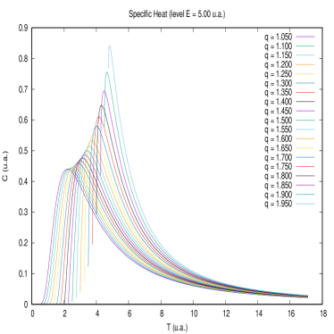
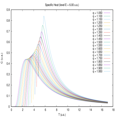
Figure 1: Temperature dependence of the specific heat (in arbitrary units) for a two level quantum system for some values of the $q$ and $E=5.0$ and $E=6.0$.

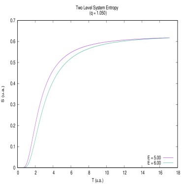
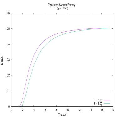
Figure 2: The temperature dependence of the entropy for $E_{0}=4.0$ and $E_{1}=5.0$, when the Tsallis’ parameter is $q=1.05$ and for $q=1.25$.

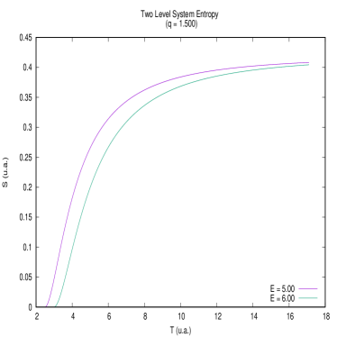
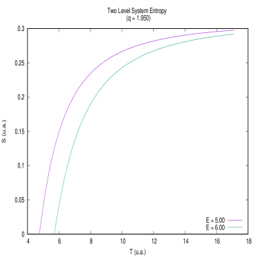
Figure 3: The temperature dependence of the entropy for $E_{0}=4.0$ and $E_{1}=5.0$, when the Tsallis’ parameter is $q=1.50$ and for $q=1.95$.

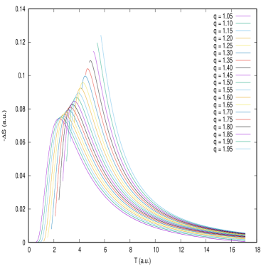
Figure 4: Temperature dependence of the magnetocaloric potential $\Delta S$ for several values of the parameter $q$. Here we use the energy gap $\delta=0.5$.

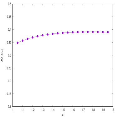
Figure 5: The $q$ dependence of the heat involved on the magnetocaloric effect (MCE). The temperature range of the MCE is from $T=0$ to $T=15$ (in arb. units).

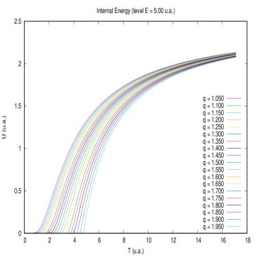
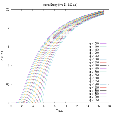
Figure 6: Temperature dependence of the internal energy (in arbitrary units) for a two level quantum system for some values of the $q$ and $E=5.0$ and $E=6.0$.

References

- (1) C. Tsallis, J. Stat. Phys. 52 (1988) 497; Braz. J. Phys. 29 (1999) 1.
- (2) C. Tsallis, Introduction to non-extensive statistical mechanics: approaching a complex world, Springer-Verlag New York, 2009.
- (3) M. Gell-Mann, C. Tsallis, non-extensive entropy: Interdisciplinary applications, Oxford University Press, USA 2004.
- (4) P. Bak, C. Tang, and K. Wiesenfeld, Phys. Rev. Lett. 59 (1987) 381.
- (5) M. Paczuski, S. Maslov, and P. Bak, Phys. Rev. E 53 (1996) 414.
- (6) M. L. Lyra and C. Tsallis, “Nonextensivity and Multifractality in Low-Dimensional Dissipative Systems,” Phys. Rev. Lett 80 (1998) 53.
-
(7)
Y. Huang, H. Saleur, C. Sammis and D. Sornette, “Precursors,
aftershocks, criticality and self-organized criticality”,
Europhys. Lett. 41 (1998) 43;
H. Saleur, C. G. Sammis and D. Sornette, “Discrete scale invariance, complex fractal dimensions, and log-periodic fluctuations in seismicity”, J. Geophys. Res. 101 (1996) 17661. - (8) A. Krawiecki, K. Kacperski, S. Matyjaskiewicz and J. A. Holyst, “Log-periodic oscillations and noise-free stochastic multiresonance due to self-similarity of fractals”, Chaos, Solitons and Fractals 18 (2003) 89.
-
(9)
J. Bernasconi and W. R. Schneider, “Diffusion in random
one-dimensional systems”, J. Stat. Phys. 30
(1983) 355;
D. Stauffer and D. Sornette, “Log-periodic oscillations for biased diffusion on random lattice”, Physica A 252 (1998) 271;
D. Stauffer, “New simulations on old biased diffusion”, Physica A 266 (1999) 35. - (10) B. Kutnjak-Urbanc, S. Zapperi, S. Milosevic and H. E. Stanley, “Sandpile model on the Sierpinski gasket fractal”, Phys. Rev. E 54 (1996) 272; R. F. S. Andrade, “Detailed characterization of log-periodic oscillations for an aperiodic Ising model”, Phys. Rev. E 61 (2000) 7196; M. A. Bab, G. Fabricius and E. V. Albano, “Critical behavior of an Ising system on the Sierpinski carpet: A short-time dynamics study”, Phys. Rev. E 71 (2005) 036139; H. Saleur and D. Sornette, “Complex Exponents and Log-Periodic Corrections in Frustrated Systems”, J. Physique I 6 (1996) 327.
- (11) C. Tsallis, L. R. da Silva, R. S. Mendes, R. O. Vallejos and A. M. Mariz, “Specific heat anomalies associated with Cantor-set energy spectra”, Phys. Rev. E 56 (1997) R4922.
- (12) R. O. Vallejos, R. S. Mendes, L. R. da Silva and C. Tsallis, “Connection between energy spectrum, self-similarity, and specific heat log-periodicity”, Phys. Rev. E 58 (1998) 1346.
- (13) D. Sornette, A. Johansen, A. Arneodo, J.-F. Muzy and H. Saleur, “Complex Fractal Dimensions Describe the Hierarchical Structure of Diffusion-Limited-Aggregate Clusters”, Phys. Rev. Lett. 76 (1996) 251.
- (14) Y. Huang, G. Ouillon, H. Saleur and D. Sornette, “Spontaneous generation of discrete scale invariance in growth models”, Phys. Rev. E 55 (1997) 6433.
-
(15)
D. Sornette, A. Johansen and J.-P. Bouchaud, “Stock Market Crashes,
Precursors and Replicas”,
J. Physique I 6 (1996) 167;
N. Vanderwalle, P. Boveroux, A. Minguet and M. Ausloos, “The crash of October 1987 seen as a phase transition: amplitude and universality”, Physica A 255 (1998) 201;
N. Vanderwalle and M. Ausloos, “How the financial crash of October 1997 could have been predicted”, Eur. J. Phys. B 4 (1998) 139;
N. Vanderwalle, M. Ausloos, P. Boveroux and A. Minguet, “Visualizing the log-periodic pattern before crashes”, Eur. J. Phys. B 9 (1999) 355;
J. H. Wosnitza and J. Leker, “Can log-periodic power law structures arise from random fluctuations?”, Physica A 401 (2014) 228. - (16) E. M. C. Abreu, N. J. Moura Jr., A. D. Soares and M. B. Ribeiro, “Oscillations in the Tsallis income distribution,” arXiv: 1706.10141 (q-fin.EC).
- (17) A. D. Soares, N. J. Moura Jr. and M. B. Ribeiro, Tsallis statistics in the income distribution of Brazil,” Chaos, Solitons and Fractas 88 (2016) 158.
- (18) P. A. Alemany and D. H. Zanette, Phys. Rev. Lett. 75 (1995) 366; 77 (1996) 2590; M. O. Caceres and C. E. Budde, Phys. Rev. Lett. 77 (1996) 2589; C. Tsallis, S. V. F. Levy, A. M. C. de Souza, and R. Maynard, Phys. Rev. Lett. 77 (1996) 5442; 77 (1996) 5442(E).
- (19) N. Ito and C. Tsallis, Il Nuovo Cimento, 11 (1989) 907.
- (20) C. Anteneodo and C. Tsallis, J. Mol. Liq. 71 (1997) 255.
- (21) C. Tsallis, Chaos, Soliton and Fractals 13 (2002) 371. R. Silva and J. S. Alcaniz, Physica A 341 (2004) 208.
- (22) C. Tsallis and A. M. C. de Souza, “Nonlinear inverse bremsstrahlung absorption and non-extensive thermostatistics,” Phys. Lett. A 235 (1997) 444.
- (23) F. A. B. F. de Moura, U. Tirnakli and M. L. Lyra, “Convergence to the critical attractor of dissipative maps: Log-periodic oscillations, fractality, and nonextensivity”, Phys. Rev. E 62 (2000) 6361.
- (24) G. Wilk and Z. Wlodraczyk, Tsallis distribution with complex nonextensivity parameter , Physica A 413 (2014) 53.
- (25) C. Tsallis, Chaos, Soliton and Fractals 6 (1995) 539.
- (26) V. K. Pecharsky and K. A. Gschneidner, Jr., Phys. Rev. Lett. 78 (1997) 4494.
- (27) I. S. Gradshteyn and I. M. Ryzhik, Table of integrals, series and products, San Diego: Academic Press, Seventh Edition, 2007.